Download User Manual - BGSU RNA group - Bowling Green State University

1
Ribostral: An RNA 3D alignment analyzer and viewer based on
basepair isostericities
1. Introduction
Ribostral (Ribonucleic Structural Aligner) is a suite of programs designed to integrate known
structural data with homologous sequence alignments, with the purpose of evaluating the quality
of the alignments and guiding efforts to improve them. The main GUI (Graphical User Interface)
of this program provides an expandable user- friendly platform through which other related
programs can be run. The related programs gather and analyze atomic resolution structure data,
parse and automatically align sequences, and perform other manipulations on sequence
alignments including extracting sub-alignments corresponding to individual motifs or domains,
removing repeated sequences from an alignment to build a “unique” alignment with higher
phylogenetic diversity, and creating a .fasta alignment file from .mat, which is another alignment
format used by Ribostral. These tools are covered in detail at the end of this manual. The main
functions of the program, namely analyzing, evaluating, and viewing RNA sequence alignments
are discussed first.
RNA sequence analysis programs are common, but none of them provides the valuable structural
information provided by ribostral. One of the most widely used editors for manual alignment of
RNA sequences is the program BioEdit, which runs under Windows platforms (1). BioEdit reads
a sequence alignment file and allows the user to choose pairs of nucleotides one pair at a time
and display substitution (covariation) patterns for them (in BioEdit, this is called Mutual
Information Examination). The resulting substitution table, however, provides no description of
what the observed substitution patterns mean in terms of structure. BioEdit does provide one
kind of link between sequence alignments and structure: if the sequence alignment contains a
“mask” describing cis Watson-Crick nested basepair, BioEdit will color nucleotides in the
alignment in terms of how well they conform to the basepair fa mily. A mask is a representation
of the locations of basepairs occurring between nucleotides represented in the sequence
alignment, with paired characters such as "(" and ")" indicating the positions of basepairs in the
alignment. BioEdit however does not provide such information for any of the other eleven or so
families of edge-to-edge interactions that are possible between basepairs, comprising about one
third of all interactions (2). BioEdit is designed to be primarily an alignment editor and viewer,
and not a tool for structural alignment of RNA the way Ribostral is. Coseq, a program that runs
under UNIX platforms, measures substitution patterns of basepairs without using any structural
information (Massire and Westhof, unpublished). The user then needs to analyze the structure
manually to see if sequence substitution patterns agree with it. Finally, S2S is another more
recent UNIX program that dynamically displays parts of structure, creates full 2D annotations of
them, and shows corresponding positions in sequence alignments in an alignment editor (3).
However, it too does not evaluate alignments based on isostericities of basepairs formed in
structure the way Ribostral does.
Ribostral, which runs under multiple platforms, can either be used like other sequence analysis
programs, i.e., to simply provide substitution patterns of basepairs in a sequence alignment
2
without any relation to structure, or can be used as the much more powerful tool that it is
designed to be: to provide substitution patterns, and at the same time superimpose structural
information on top of the substitution patterns to make sense of it. Ribostral does that by coloring
substitution patterns of each basepair in a way that reflects the edge-to-edge family and the
isosteric subfamily it belongs to (4). Even in its more simple usage as a program that provides
sequence substitution analysis without the use of 3D structural information, Ribostral is more
convenient than other programs, because it allows for simultaneous analysis of lists of basepairs
and produces a single and easily portable HTML output, without having to input nucleotide
numbers of interest one position at a time. Interactive position-by-position analysis is also
possible, where in addition to what has been described above, an integrated structure viewer is
also available. In addition to providing substitution information for basepairs, Ribostral is also
capable of analyzing substitution patterns for more than two nucleotides at once, such as base
triples, quadruples, and so on. The sequences of whole motifs can be analyzed this way, as will
be shown below.
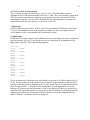
1.1. Supported platforms and deployment process
Ribostral is designed and fully tested under Windows XP. It is free and can be obtained from
http://rna.bgsu.edu/Ribostral. The program is distributed in two forms: MATLAB source files
capable of running on any PC or MAC platform with MATLAB version 7 SP3 or higher (with
loss of some non-essential options on MAC), or a stand-alone program capable of running under
the PC platform, after installation of a free compiler provided by Mathworks (details can be
found here). Figures used in this text are based on the Windows XP version with system
appearance set to Windows Classic style. Upon downloading the MATLAB source files or the
stand-alone version, the user will end up with the specific hierarchy of folders shown in Figure 1.
3
Figure 1. Ribostral default installation subdirectories. Using folders marked with asterisk (*) is optional; on
Windows platforms, these are the locations where Ribostral starts browsing for the corresponding input files.
1.2. Disclaimer
No guarantee, expressed or implied, is made as to the suitability of this software for any purpose,
computer, or person. The author shall not be held responsible, nor be liable for any damage
occurring in any way to equipment or health while using this software.
Author contact information: Ali Mokdad, M.D., Ph.D., Department of Biological Sciences,
Bowling Green State University, Bowling Green, Ohio 43403. Email: [email protected].
2. Executing Ribostral
Ribostral can run as a GUI or as a script under MATLAB (by running the program
ribostralNoGUI; follow the header information to point to your files of interest). The following
discussion concerns mainly the default GUI version.
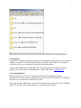
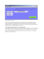
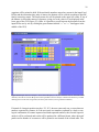
The startup window of Ribostral is a blank GUI with three menu options: File, Tools, and Help
(Figure 2). The other GUIs of the program are activated from this window.
4
Figure 2. Ribostral’s main GUI.
To avoid ambiguity, the GUI only displays options that are allowed at the specific stage of the
analysis. For example, before doing any analysis the user needs to load a sequence alignment file
on which the analysis will be performed. So initially, the GUI does not display the buttons that
start the analysis. These buttons will appear only after the sequence alignment file is loaded into
the program. To provide additional help for the user, the upper right- hand corner of the main
GUI is reserved for messages describing the status of the program, any errors in execution, or
hints on how to proceed further.
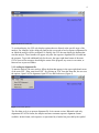
2.1. Loading an alignment file
To start the analysis, the user needs to follow the hint that appears in the upper right- hand corner
of the main GUI: “Hint: start from FILE”. By clicking on “File” from the menu bar, the user sees
the options: Open FASTA alignment, Open NT list, and Preferences (Figure 3).
Figure 3. File menu options.
The first thing to do is to open an alignment file. In its current version, Ribostral reads only
alignments in FASTA format, the simplest and most common sequence alignment format
available. In this format, each sequence is represented by a header line preceded by the symbol
5
“>” and one or more sequence lines. Upon choosing “Open FASTA alignment” from the File
menu, the user can browse the local drive for alignment files (Figure 4).
Figure 4. Browsing for an alignment file.
On PC machines, the browser window initially starts looking for alignment files in the folder:
“< installation directory> \FASTA_alignments” (refer to Figure 1). Here, there are two main
options: reading a raw alignment file in its text form (with extensions such as .fasta, or .txt), or
reading a MATLAB data file (.mat) which is derived from the raw alignment file. This last
option is processed faster by Ribostral, especially if the alignment of interest contains thousands
of sequences, like the 16S rRNA alignments. A .mat file is created after a FASTA alignment is
read for the first time. It is saved in the same directory and under the same name except for the
extension. Time can then be saved by reading the data file instead of the text file the next time
the same alignment is used. Note that a new data file is only created if no data file with the same
name is already present in the directory. Therefore, if the raw FASTA alignment is deliberately
modified in any way, the old .mat file referring to it needs to be deleted to allow for its recreation. Notice that when a FASTA format file is read, all characters indicating unknown
nucleotides (“N”, “n”, “O”, and “o”) are transformed into “o”, and all other characters are
capitalized. When analyzing basepairs, Ribostral only recognizes dashes (“–”) which represent
gaps or deletions, o’s, and the four RNA nucleotide letters A, C, G, and U as valid characters in
sequences. When analyzing longer motifs, the program recognizes all characters.
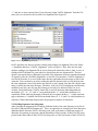
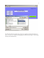
2.2. Dividing Sequences into Subgroups
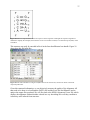
After choosing the alignment file of interest, Ribostral looks in the same directory for an Excel
file called “KnownFASTAFilenames.xls”. This is an optional user-created Excel sheet that gives
additional details about the FASTA file being read, such as the names of different groups (or
domains) of organisms it represents, and the boundaries of these groups. If this Excel file is not
present in the same folder as the FASTA file being read, or if the exact name of the FASTA file
6
being read cannot be found in the Excel file, this information will be ignored and all FASTA
sequences in the alignment will be considered as one group. The analysis of specific subgroups
(such as phylogenetic domains) will not be possible later. Figure 5 shows the format of the
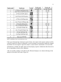
“KnownFASTAFilenames.xls” file and the info rmation it contains.
Figure 5. A snapshot of the “KnownFASTAFilenames.xls” file. The highlighted entry (number 6) is the FASTA file
analyzed in this manual.
The Excel file is organized in the following way: The first column contains the exact names of
“known” FASTA alignments; the second column contains the names of the subgroups the
FASTA alignment contains separated by empty spaces; and the third column defines the limits of
these subgroups in the order of their names, separated by empty spaces. The highlighted file
(entry 6, 5S_ABE_2004_UNIQUE.fasta) is the one used for the sample study in this manual. It
contains sequences from the phylogenetic subgroups: archaea (sequences 0+1 to 39), bacteria
(sequences 39+1 to 390), and eukarya (sequences 390+1 to 667). To ignore the first sequence in
the alignment (if it is a structure mask for example, or if it is a reference sequence that does not
belong to the subgroup), “1” can be placed instead of “0” in the third column. In that case, the
program still reads the first sequence but does not include it in the analysis.
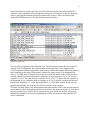
The main GUI then displays any known details associated with the FASTA file and also unlocks
some buttons or check boxes that permit the user to analyze the alignment (Figure 6). Note that if
this step (loading a new FASTA file) is repeated at any stage during the analysis, all previous
data that corresponds to previously read alignments will be erased from memory and the GUI
will be reinitialized.
7
Figure 6. GUI changes when an alignment file is successfully loaded. The text box in the middle displays the name
of the sequence file in memory.
At this stage, two options are possible for carrying out sequence (and optionally structure)
analysis: analyzing a list of nucleotides (with or without structure data) for the complete
sequence analysis of all positions listed in it, or interactively and directly analyzing individual
positions on screen. The first option is covered first.
2.3. Preparations for the analysis of a list of nucleotides
After loading a FASTA file, the user can load an Excel file containing a list of the nucleotides of
interest. This is done by activating the option “Open NT list” from the File menu. A browser
opens and on PC platforms search for Excel files starts in the local directory “<installation
directory>\NT_lists” (Figure 7).
8
Figure 7. Browsing for an Excel nucleotide list.
The NT list Excel file must contain names of the source organisms and nucleotide numbers of
interest. The first row is a header row and anything in it will not be read. Figures 13 and 14 show
what such a file should look like.
9
Figure 8. Nucleotide list for analysis. This Excel list from 23S rRNA allows the sequence analysis of four
nucleotide positions simultaneously.
Figure 9. Basepair list for analysis. This Excel list from 5S rRNA includes structural data about some of the
basepairs (to show that structural data is optional).
10
As seen in Figures 8 and 9, the first column of the Excel sheet contains the name of the reference
organism for that row, and subsequent columns contain the nucleotide numbers to be analyzed.
The name must be the full name or part of a name (case insensitive) present in the loaded
FASTA alignment file. It does not necessarily need to be the beginning of the name (e.g.
“Halomari” can be used if the actual name in the FASTA alignment is “Eu_halomari”). If several
FASTA comment lines share this name, the first of the occurrences will be considered as the
reference organism (e.g. if “halo” is used, and it is present three times in the sequence alignment,
first as “EU_HALOJAPO”, then as “Eu_halomari” and then as “Eu_halomedi”, the first will be
used). It is advisable for the user to manually check sequence names in the FASTA file to
prevent inadvertent reference to unintended organisms. The most common error is caused by
incorrect spelling of the source organism in the NT list Excel file; if such a spelling cannot be
found in the FASTA file an error message will appear and the program will stop. If universal
numbers for the alignment are desired the word “universal” can be used instead of an organism
name (similar to entry 8 in Figure 9).
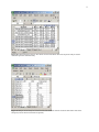
Structural information (i.e. basepair type) is allowed only for basepair lists. These are lists
comprising two columns of nucleotide numbers, like the one shown in Figure 9. Basepair types
are named by reference to the interacting edges of the nucleotides. These are the Watson-Crick
edge (W), Hoogsteen edge (H), and sugar edge (S). Edge-to-edge interactions in addition may be
cis (c) or trans (t) with respect to the glycosidic bond. This gives rise to twelve main families of
basepairs (2,4), and some intermediate families (5), only one of which with currently
characterized isostericity matrix (the bifurcated cWW/tWH family). These thirteen basepair
types are coded as follows in order for Ribostral to understand them (case insensitive for all
except tSs, because it is a directional interaction with asymmetric isostericity matrix): cWW,
tWW, cWH, tWH, cWS, tWS, cHH, tHH, cHS, tHS, cSS, tSs, and bif. Asymmetric codes (such
as cWS) can be reversed, so in the table if nucleotides 22 and 26 in this order are coded as tSW,
this is the same as 26 and 22 being tWS (see Table 1 for a definition of all the basepair codes
used by Ribostral). Ribostral always presents data about basepairs as one of the thirteen codes
listed above (and not the reverse form).
11
Table 1. Basepair codes used in Ribostral. The last column shows the codes used for constructing the structural
mask in Alignment Viewer, discussed later in text.
If the type of basepairing is known for a pair of bases, the output of the sequence analysis will be
colored to indicate its isosteric subfamilies, so the investigator can determine whether the aligned
nucleotides for each sequence represent isosteric or near- isosteric substitutions. If no structural
information is available, the table output will only display sequence substitution data observed in
the corresponding columns of the alignment.
After successfully reading a nucleotide list file, Ribostral displays a new button allowing for the
analysis of the whole list at once (Figure 10).
12
Figure 10. The main GUI after successful loading of a nucleotide list file. The status bar (upper right hand corner)
displays “NT list loaded” and the new button “NT list analysis” becomes available.
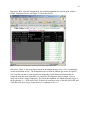
2.4. Analyzing a list of nucleotides
Upon activation of the button “NT list analysis” the program takes each row of the Excel NT list
file and counts the number of each substitution of its nucleotides in corresponding columns of
the alignment. This process may take a few minutes for long lists of nucleotides or for large
alignments. The MATLAB command prompt (or the DOS prompt if the compiled stand-alone
version of Ribostral is executed) displays different messages and counters indicating the status
and progress of the analysis. Upon successful execution, output files are created in the folder
“<installation directory> \Output” (refer to Figure 1), with descriptive names indicating the NT
list file and the alignment file they represent. At the same time a new button providing a quick
link to the main output file will also appear on the main GUI.
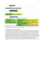
3. Types of output files and their interpretations
Depending on the type of input NT list, several types of output files are possible (Figure 11). The
following sections discuss each type of these output files in detail.
13
Figure 11. Output files produced depending on input files analyzed. The first output file in each case is the “main”
file accessed directly by clicking the button “Display list results” on the main GUI. Outputs indicated by asterisks
(*) are produced optionally by changing the program preferences.
3.1. Output files for a non-basepair list
If the input NT list is not a list of basepairs but a list of nucleotides forming distinct motids (such
as the one shown in Figure 8), two text output files will be created, one giving counts and the
other percentages of sequences tha t share a common pattern (Figure 12). The patterns are listed
in alphabetical order. To clarify this, the following example from Figure 12 is considered. The
first entry in the Figure (highlighted) shows that in the archaeal part of the alignment, nucleotides
corresponding to Haloarcula_marismortui local numbers 545, 611, 529, and 14 (in this order) are
88% GUGC and 12% GUGo. From this one can deduce that Nucleotides 545, 611, and 529 are
GUG in 100% of the cases, and so on. The values in the percent output file are rounded
according to the preferences of the user (Ribostral preferences will be discussed in detail later).
14
Figure 12. Percent output text file created upon sequence analysis of an NT list. Sequence patterns are listed in
alphabetical order. A similar output file with counts instead of percents is also created. This analysis is for the NT
list shown in Figure 8.
3.2. Output files for a basepair list
In case the Excel input NT file gives a list of basepairs from an atomic resolution structure,
Ribostral generates output files that are better tuned and more informative for this kind of input.
These include colored HTML outputs in the form of tables with sequence substitution values.
The tables use different background colors to indicate for each basepair whether observed
substitutions are isosteric, near- isosteric, heterosteric, or forbidden as compared to what is
observed in the structure. By default, three HTML output files (and a fourth text output in case
the input Excel list is a basepair list with structure information) are produced upon the analysis of
a basepair list (see Figure 11). The main output file accessed directly by the “Display list results”
button on Ribostral is the percent covariation file whose name ends with “_COV_Percents.html”.
A similar “_COV_Counts.html” file shows the counts instead of percents. Figure 13 displays a
15
snapshot of such an output. A third file (ending with “_SEQ.html”) displays the names of
organisms giving rise to the values in the first two output files. The positions of the names
correspond to the values observed, as clarified in Figure 14. Note that the basepair identity
observed in structure is indicated by bold font in the corresponding cell.
16
Figure 13. Percent output HTML file created upon phylogenetic analysis of an basepair list. A similar output file
with counts instead of percents is also created. This analysis is for the NT list presented in Figure 8 above.
17
Figure 14. Matching sequence values and names. The “_COV_Counts.html” output file (left panel) displays the
sequence counts, and the corresponding “_SEQ.html” (right panel) displays the names of sequences. Note the value
indicated by the black arrow in both outputs: The left panel shows that there are three bacterial counts for AA
occupying the position A3/G21 (halomari local numbers). The right panel shows that these three counts come from
the sequences of G_complan, P_palmata, and S_vulgare.
The output files have two purposes: First, to display substitution patterns corresponding to each
BP position analyzed, and second, to provide information about how well each of these positions
in alignments agrees with 3D structure. Based on this, if there are any potential mistakes in the
alignment they are easily pinpointed for their manual correction with available sequence editors.
All three HTML output files mentioned start with a total score assigned for each phylogenetic
subgroup in the alignment (in this case the subgroups are the three domains: archaea, bacteria,
and eukarya). Each subgroup will have its own results printed on a separate line in the
substitution tables. The areas in Figure 14 indicated by the black arrows for example represent
the substitutions in eukaryal sequences of the basepair A3/G21 (using halomari local numbers).
On top of each table that represents a basepair position the following information is provided:
18
The names of the subgroups in the order they are analyzed, the numbers of sequences in each
subgroup, the count of forbidden substitutions present in the table (in red color, with the letter F
following the value), the count of gaps present including gaps on both sides or just on one side
(in gray, with the letter G following the value), the count of isosteric substitutions (in blue, with
the letter I following the value), nearly- isosteric substitutions (in cyan, with the letters NI
following the value), non- isosteric but not forbidden substitutions that we refer to as heterosteric
substitutions (in pink, with the letter H following the value), and finally individual scores of each
subgroup at that basepair position.
The score is a value describing how structurally “acceptable” the sequence substitutions at
analyzed basepair positions are. This is based on the measure of how structurally compatible
these substitutions are with the basepair in the reference organism, which is typically the
organism with known structure. The individual basepair scores are currently calculated based on
an ad hoc formula derived from experience with structures and knowledge of the patterns of
allowed substitutions for each type of basepair. This formula can be easily modified by the user,
by manually entering desired weight parameters in the file “<installation
directory>\Ribostral\SCORES.txt”. The formula used throughout this text is:
Individual BP score = c * SUM(3I + 2NI – H – 2F – 2G1 – 3G2) / number of sequences
Where c is the correction coefficient: c = 100 / (Highest positive weight), in this case c =100/3.
I, NI, H, F, G1 and G2 are the counts of sequences having substitutions that are isosteric, nearlyisosteric, heterosteric, forbidden, gap on one side, or gaps on both sides respectively. The
Highest positive weight is 3 in this case. The correction coefficient c insures that the maximum
score is +100 (in this case, the minimum score when all substitutions are gaps on both sides is –
100, but that is not always the case depending on the formula used). The formula used here is
asymmetric: unfavorable terms that contribute to its reduction are more numerous and weigh
slightly more than favorable terms that contribute to its increase. But for our purposes, this is not
a critical point. What is important is to easily identify low-scoring spots in the alignment to guide
manual realignment efforts. To better locate these trouble spots in the alignment, the score is
printed in red if it is worse than a certain threshold (i.e. if it is below zero, which is the score in
case no structural data is available) and in black otherwise. The total score printed at the top of
each HTML output file is an adjusted sum (sum divided by number of basepairs studied) of the
individual BP scores in the study (so it is actually an average of the individual scores). This
means that its maximum is also +100 and its minimum, in case the formula presented here is
used, is –100.
Note that another valid formula used can be something like:
Individual BP score = c * SUM(2I + NI – 3F) / number of sequences
Both formulas are ad hoc and the difference between their weights is not essential. The ease of
reading and understanding normalized values between +100 and –100 or –150 is the reason for
using a correction coefficient.
19
The most obvious and important element of the HTML output files discussed thus far is the
background color patterns that appear in their tables. These colors reflect the isostericity matrices
of the thirteen characterized families of basepairs. Each family has its own pattern of isosteric,
nearly- isosteric, heterosteric, and forbidden substitutions. Boxes with the same colors are
isosteric. Boxes that are nearly- isosteric with each other have “similar” colors. There are five
groups of these “similar” colors: pink/red/orange, red/orange/yellow (so substitutions with pink
and yellow backgrounds are not nearly isosteric to each other), blue/cyan, dark green/light green,
and brown (Figure 15). Forbidden boxes are colored in dark gray, and gaps in light gray. Boxes
with non-similar colors indicate that they are heterosteric to each other. If the basepair family for
a certain basepair is not specified, all nucleotide boxes in its table will be colored in neutral beige
(like the second BP listed in Figure 13).
20
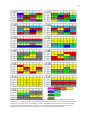
Figure 15. Basepair families and their isosteric subfamilies. Gray colors indicate forbidden combinations of
nucleotides, i.e., combinations that cannot form basepairs due to steric clashes or incompatible distribution of Hbond donor or acceptor atoms. In each family, isosteric subfamilies have the same color, and nearly isostericfamilies have similar colors (the five “similar” color groups are shown on the bottom right corner). Letters
correspond to the original reference (4). Asterisk (*), corrected from the original reference.
21
One more output file is produced by default in case a basepair input list with structure
information is analyzed. This is the “_Statistics.out” file, which is best viewed with Microsoft
Excel or WordPad. This output summarizes some of the results by stating the percentage of
basepairs analyzed that have mostly allowed substitutions (containing <10% forbidden or gaps),
the percent of basepairs that have >10% forbidden substitutions, and the percent of basepairs
having >10% of sequences with gaps at their positions. It also shows the percent of basepairs
among the ones mostly allowed that have only isosteric substitutions. Instead of the total score
which is just one value that describes the quality of the alignment studied, this output file gives a
more quantitative measure of the alignment quality.
When a Basepair list is analyzed, a button labeled “Plot scores” also appears on the main GUI.
When activated, this allows the user to quickly analyze the scores of each basepair and define
places of misalignment or motif swaps (Figure 16).
Figure 16. Score plots for the archaeal 5S rRNA alignment. The red curve describes the scores of corresponding
basepairs, and the blue line represents the average score (or total score as defined in this text) for the whole
alignment based on the basepair list provided. By modifying the ad hoc formula according to which scores are
calculated (this can be done by changing parameters in the “SCORES.txt” file), the user can plot any combination of
one or more aspects of the alignment, such as percent isosteric substitutions, percent isosteric and near-isosteric
substitutions, and so on.
22
3.3. Ribostral Alignment Viewer
There are additional output files not produced by default that can be obtained by changing the
Preferences under the File menu options. The reason for not producing those output files by
default is not to overwhelm the casual user with too many output files, and not to unnecessarily
extend the execution time.
If the “AlignViewer” option is selected in Preferences, an HTML-format alignment viewer is
created where the sequence alignment is shown in colors indicating substitutions that are
compatible with the 3D structure and those that are not. This tool is the first of its kind taking
into consideration all thirteen families of basepairs instead of just the classical cis Watson-Crick
family. The sequences in the Alignment Viewer are colored in a way to describe how well each
column (more precisely, each pair of columns) in the alignment agrees with structure (Figure 17).
Basepairs from each sequence are colored individually based on their isosteric agreement with
the homologous basepair from the reference sequence, which is usually the sequence with known
3D structure. If the substitution pattern is isosteric to the one in the reference sequence it is
colored in green, if it is nearly- isosteric to it, it is colored blue, heterosteric is pink, forbidden is
red, gap on one side is dark gray, and gap on both sides is light gray. If no basepair information
is available the nucleotides are printed in black (these color assignments can be modified by
changing the MATLAB script file “mColorCode.m”). For easy interpretation, the color scale is
printed at the top of the alignment viewer HTML file. Thanks to this tool, it is now possible to
look at the sequence alignment and directly get a good idea about whether the alignment is
structurally valid or not, and where the major areas for local alignment mistakes (or motif swaps)
are located. Note that if base triplets are present (i.e., two basepairs with one nucleotide in
common), the basepair listed earlier in the Excel BP list file takes priority in coloring. If the user
prefers to give priority to cWW interactions for example, then these should be listed first in the
BP list.
23
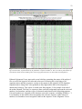
Figure 17. Ribostral HTML alignment viewer. The visible part of the 5S alignment describes how well sequences
agree with structure, represented here by Eu_Halomari, or sequence number 11. The color code is printed at the top.
Note that the whole content including colors can be copy/pasted into Excel or other editors for manipulation.
Ribostral Alignment Viewer starts with several title lines containing the names of the analyzed
files as well as the legend of all codes and colors used. Following this is the listing of all
organism names and their sequences, exactly as they appear in the original FASTA alignment.
Organism names cha nge their color gradually as they approach the limit of the subgroup or
domain they belong to. This is how it is made clear that sequence 39 for example is the end of
the archaea domain. The first five sequences (those on black background) represent the universal
numbers, local numbers, and three types of structural masks that describe basepairing patterns.
Universal numbers are assigned to each character seen in the sequence, including all indels (“–”).
Local numbers are the numbers that correspond to the reference sequence; unlike universal
numbers, local numbers are not assigned to indels in this sequence. In the Alignment Viewer
24
only decimal representatives of local numbers are listed, i.e. the first “1” stands for 10, the first
“2” stands for 20, and so on until the first “0” is seen, which stands for 100. After that the
numbering cycle is repeated, so the second “1” stands for 110, the second “2” stands for 120, and
so on.
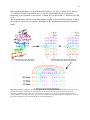
The structural masks describe basepairing patterns reported in the Excel BP list directly on top of
the sequences. Figure 18 is a schematic description of the information represented by structural
masks.
Figure 18. Schematic explanation of structural masks. These are one dimensional representations of structure. The
example shown here is from Helix 95 containing the sarcin/ricin motif in the large ribosomal subunit of H.
marismortui (pdb file 1S72). Color codes correspond to basepairs. Note that the 13D and 3D masks may have
several symb ols overwriting each other; only one of the cyan RG and ][ symbols displayed in this Figure on top of
each other is displayed in the 13D and 3D masks produced by Ribostral.
25
The 2D mask describes only nested basepairings, irrespective of their geometric families (most
of these would be helical cWW basepairs). Each nested basepair (one which does not cross in 2D
with other basepairs) is represented by the two parentheses symbols “(” for its opening or 5’
nucleotide and “)” for its closing or 3’ nucleotide. The 3D mask is the same as the 2D mask, but
in addition to representing nested basepairs it also represents other non- nested basepairs using
the bracket symbols “[” and “]”. When one nucleotide forms more than one basepair by using
more than one of its edges at once (e.g. in base triplets), the number of bracket symbols of the
opening and closing type may not be equal. Therefore, it is not possible from this mask alone to
know which opening brackets correspond to which closing brackets. Another limitation of both
the 2D and 3D masks is that they do not tell anything about the type of basepairs formed. The
13D mask is designed to solve this problem. Here, instead of just one or two pairs of symbols
representing opening and closing of basepairs, thirteen different pairs of symbols are used to
represent all known families. These codes are AB for the cWW family, CD for tWW family, and
so on (see Table 1). Since some families also are not symmetric (C/G cWS has a different
meaning than C/G cSW), uppercase symbols and lowercase symbols are used to indicate the
direction of the interaction. The symbols must be read from uppercase to lowercase direction
whenever the interaction is asymmetric, with the uppercase symbol referring to the base edge of
higher priority (edge priority is assigned in the order W, H, S). Thus, if an interaction exists
between columns (universal numbers) 38/42 and is represented by kL, this means that
nucleotides occupying these positions form a tSW interaction in the source organism (or
structure). This is the same as saying that 42/38 is a tWS (or Lk) interaction. The 13D mask has
the same limitation as the 3D mask, in that finding matching opening and closing symbols is not
always straight forward. Using the 2D mask together with the other two masks makes it easier to
at least find nested pairs.
3.4. Other output formats
Ribostral can also create other output files upon request (by checking the option “GU special” in
Preferences). These files represent another way of classifying some similar isosteric groups
together, the way the G/U wobble basepairs are analyzed in our previous work (6). Ribostral
scripts can easily be modified to produce other similar outputs.
4. Interactive analysis of nucleotides
Besides analyzing lists of nucleotides or basepairs at once and producing dedicated output files
that describe their results, Ribostral is also capable of analyzing nucleotides of interest one by
one and directly displaying their results on screen. This can be done by activating the button
“Interactive analysis” from the main GUI, which starts a new GUI window (Figure 19). This
option becomes possible only after successful loading of a FASTA alignment file. If a BP list file
is also loaded before the interactive analysis is activated, the new GUI will have more options
and information extracted from that file. In the following text we will discuss the options
available in case a BP list is loaded before activating the interactive analysis GUI.
26
Figure 19. Initial screenshot of the interactive analysis GUI. Here, both a FASTA file and an NT list file were
loaded from Ribostral main GUI before starting this GUI. If only a FASTA file was loaded, some of the options or
buttons seen here would not have been made visible.
The interactive analysis tool is a powerful tool providing yet a new array of functions not
provided by the list analysis tools discussed in previous sections. After specifying the right
choices (such as source organism name, domain of interest, etc…) the user can either analyze a
specific family of basepairs, or analyze a particular position.
4.1. Interactive analysis of a family of basepairs
The right-hand side of the interactive analysis GUI contains the options and buttons capable of
gathering statistics about a whole family of basepairs at once. This option is only possible if the
user has loaded a basepair list before opening this GUI. An example of what can be done here is
the analysis of all the occurrences of the tHS family in the archaeal part of the 5S rRNA
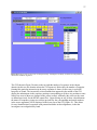
alignment. The result of such an analysis is shown in Figure 20.
27
Figure 20. Analysis of all occurrences of a basepair family. All basepairs of family 10 (tHS) are analyzed here in
the archaeal 5S rRNA alignment.
The GUI shown in Figure 20 states on the top right the number of sequences in the chosen
domain (in this case the domain archeae has 39 sequences). Below that, the number of basepairs
forming this particular interaction in the source organism is shown. In this case six such tHS
basepairs are found. The isosterically colored buttons that appeared in the middle of the GUI
display the substitutions in the sequence positions corresponding to all these six positions at once.
Notice how most of them are clumped in the yellow isosteric subfamily (the colors are the same
as defined previously for the HTML output files). Upon clicking on any of these colored buttons
the names of sequences giving rise to them (preceded by the corresponding nucleotide numbers
in the source organism) will be displayed in the lower part of the GUI (Figure 21). This allows
for easy identification of organisms with potential mistakes in their alignments, so that the
investigator can realign them by hand.
28
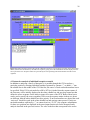
Figure 21. Getting sequence names with specific substitution patterns. Upon clicking any button in the substitution
matrix (button GU is clicked here), the names of sequences giving rise to the substitutions become displayed in the
lower part of the GUI. Sequence names are preceded by the corresponding nucleotide numbers from the source
organism.
4.2. Interactive analysis of individual basepairs or motifs
In addition to analyzing a family of basepairs, it is possible through this GUI to analyze a
particular position by entering individual numbers separated by commas “,” or dashes “- ” into
the editable box in the middle of the GUI. But first, the source of local nucleotide numbers has to
be specified. If this GUI is activated after a BP or NT list is loaded, then the sequence name of
the first entry will be initially displayed in the white editable box and gray drop-menu box that
define the source sequence for the analysis (upper left corner of the GUI). Both of these boxes
can be used to specify the source organism, but in case the sequence names in these two boxes
are different, then the white editable box takes priority. If universal numbers are desired the word
“universal” should be typed in the white editable box and carriage return pressed. If only two
nucleotide numbers separated by “,” are entered (such as “22, 26”), the sequence substitutions
for these two positions are displayed in the same output format seen for the basepair family
analysis described in the previous section. The value in the box that corresponds to the source
29
organism will be printed in bold. If the nucleotide numbers entered are present in the input Excel
BP list and the interaction they make is known, the buttons will be colored according to their BP
family isostericity matrix. The family name also will be printed on the upper left corner. If any of
the buttons is clicked the names of sequences giving rise to the value in it are displayed in the
lower part of the GUI (Figure 22). (Note: it is possible to scroll between the basepairs from the
input BP list one by one by clicking the green buttons labeled “<<” or “>>” that appear in the
middle of the GUI).
Figure 22. Basepair interactive analysis . Notice that if the query is “22, 26” instead of “26, 22” the same result is
obtained, since this is a known BP present in the input BP list and it is always colored in the same way. The BP
identity present in the source organism (also the crystal structure) is CG (printed in bold font).
If instead of a basepair position (such as “22, 26”), the user enters only one, or more that two
numbers separated by commas, or if the user enters two numbers separated by a dash, or any
logical combination of comma-separated and dash-separated numbers, then a motif sequence
analysis will be performed and results will be produced in a different format, where the motif
pattern and its number of occurrences will be printed in text instead of the colored table. The
30
pattern present in the source sequence will also be indicated by the “<<<” sign. Once again, if
the user clicks on any one of the nucleotide patterns, the names of sequences giving rise to them
will be displayed in the lower portion of the GUI (Figure 23).
Figure 23. Motif interactive analysis. Individual nucleotides in the motif are arranged in the order of the positions
entered. Since the query here is “26-22, 37”, the letters that correspond to local number 26 of source organism is
displayed first, then those that correspond for 25, then 24, 23, 22, and finally 37. If instead of this the query was “2226, 37” the result would be displayed differently.
Finally, the interactive GUI provides a quick link to a basic structure viewer through the
activation of the button “Display 3D”. When this button is clicked the first time it prompts the
user to choose the PDB file corresponding to the sequence studied, and atomic coordinates are
read (the bigger the PDB file the slower this process). The structure of the input nucleotides is
then shown. Subsequent activations of the button within the same session display the structure
immediately.
31
4.3. Notes
1- The user can change the color distribution of the substitution table to be similar to another
basepair family. This may be important in case mistakes in the BP list are suspected, or in case
no BP family is stated, causing the whole table to be in one neutral color.
2- It has been shown that the colored GUI buttons may display the results of either a whole BP
family or an individual position. To prevent any confusion, a thin white box appears everytime
one of these two types of analyses is requested. This line surrounds the output buttons as well as
the input buttons giving rise to them. The difference can be clearly seen between Figures 20 and
21 on the one hand and Figures 22 and 23 on the other.
5. Ribostral preferences
Ribostral is a diverse program capable of dealing with data in a variety of ways. Through its
preferences, the user can enhance his experience with the program and make it do what is best
for the investigation in hands. Ribostral preferences can be accessed from the File menu of the
main GUI. They are then saved as a data file on the users disk, for easy passing between all
subordinate Ribostral GUIs. Last positions of GUIs before exiting them are also saved in this file,
so that GUIs always open in the last known position they were closed in. Figure 24 shows the
default preferences of the program.
Figure 24. Ribostral default preferences.
The preferences are divided into several categories. Round radio buttons belonging to the same
category are mutually exclusive. The first two categories, “Display Totals” and “Display
Expected”, affect only the list output files and do not affect the interactive analysis GUI. If
“Display Totals” is enabled, the totals of each row and column of the BP list output are printed
with the output (as in Figure 13). Otherwise, the totals will be left out. If “Display Expected” is
enabled, the expected value for each substitution is printed in parentheses after the observed
substitution value, as in Figure 25.
32
Figure 25. Substitution counts with expected values (in parentheses).
The expected value for each box in the table is obtained by applying the formula:
Expected (of box in row a, column b) = Sum of boxes in row a * Sum of boxes in columns b /
Table total
This value is a measure of the likelihood of observing substitutions in the specific box, based on
the values observed in the neighboring boxes.
Enabling the “Audio” option allows the program to play specific musical chimes every time an
operation is completed or an error occurs. This is useful in case a large file is being read or
analyzed. In such cases the user will be notified by the sound to carry on to the next step.
Enabling “Consider Gaps” means that the program will not ignore insertion characters (“–”) seen
in the alignment. Disabling this option not only stops the program from showing gaps in the
output, it also ignores gaps from any other calculations, such as score or percent substitution
33
calculations. The “consider Ns” option does the same thing but with characters representing
undetermined nucleotides (usually symbolized by “o”, “O”, “n”, and “N”, which as stated earlier
are all converted to “o” when the FASTA alignment file is originally read). These two options do
not affect analysis of non-basepairs, such as base triples or longer motifs.
Several rounding options are available through a dropdown menu. The choice here affects the
presentation of all decimal calculations done by Ribostral. Activating any of the “Additional
Output” options results in the production of one or two more output formats that Ribostral does
not produce by default (discussed earlier). Preferences are saved only if the “SAVE” button is
activated.
Finally, upon activating the button “Modify Score Parameters”, the file containing score
parameters (“<installation directory>\Ribostral\SCORES.txt”) is opened for editing. The
parameters entered in this file affect all score calculations. The resulting formula is shown on
screen and is also printed out in some output files every time sequence analysis is carried out.
6. Supporting tools
Ribostral provides an expandable sequence and structure analysis platform. Additional tools can
be easily and smoothly integrated into the main program. There are currently five additional
tools that allow Ribostral to do operations beyond structurally analyzing sequence alignments
(Figure 26). Each of these tools is discussed separately below.
Figure 26. Ribostral tools.
6.1. Tool 1: Generate BP list from PDB
This tool currently works only on PC platforms. PDB files are text files containing all the atomic
coordinates and related information about a structure. By analyzing this data, interacting bases
can be identified and classified into geometric families (7). Upon activation of this tool, the user
first chooses a PDB file (browsing starts from the default PDB directory associated with
34
Ribostral “<installation directory>\PDB_structures”). Then, the user is prompted to enter the
sequence name in the alignment that corresponds to this 3D structure. Ribostral then creates an
Excel BP list for each of the basepair families found in the crystal structure. It also creates a
separate Excel BP list containing all of them, and another Excel BP list containing all the noncWW ones among them together. These lists are created in the proper format to be read directly
by Ribostral and are saved in the default “<installation directory> \NT_lists” folder. Note that the
automatic classification of basepairs is not 100% accurate, so the resulting automatic lists should
be visually compared to the 3D structure and corrected where needed.
6.2. Tool 2: Align sequences
This tool opens a GUI that interfaces with automatic motif alignment programs based on a
hybrid Stochastic Context Free Grammars/Markov Ra ndom Field (SCFG/MRF) model. The GUI
facilitates some of the steps in running these programs, and allows the user to parse and align
motifs that have their SCFG/MRF nodes already characterized based on known 3D structure.
Currently, MATLAB script files still need to be modified in order to parse and align new motifs.
This tool mainly provides an easily expandable user- friendly platform for applying automatic
sequence alignment.
6.3. Tool 3: Extract parts of a FASTA file
This tool, shown in Figure 27, requires loading a FASTA file from Ribostral main GUI before it
can be activated.
Figure 27. GUI for extracting parts of a FASTA file.
The user then simply needs to indicate the motif of interest by entering its nucleotide numbers in
the editable box. All positions homologous to these numbers will be extracted from the original
alignment and saved as a new sub-alignment in FASTA format. If there are one or more commas
separating two or more groups of numbers, the sub-alignment will represent these breaks in
35
continuity by four consecutive dots (....). This continuity separation code is understood by other
Ribostral tools, such as the alignment parser tool discussed in the previous section. Naturally,
nucleotide numbers refer to the source or reference organism specified in the GUI. Similarly to
the interactive analysis GUI, in case there is disagreement between the sequence name in the
white editable box and that in the gray drop- menu box, the white editable box takes precedence.
The user can choose to ignore up to five organisms from the top of the sequence alignment (for
instance, if these are structure masks or sequences that do not belong to the same phylogenetic
group), and can choose to extract one domain or all domains at once. The extracted subalignment is saved in the same directory as the original source alignment file.
If there is more than one motif to be extracted, the user can create a tab-delimited input text file
containing the names of all of them and their nucleotide numbers for batch processing. The
nucleotide numbers should correspond to the Reference Organism Name selected in the GUI.
The input text file would look like this:
h5IL
53-56,356-358
h6IL
64-69,99-103
h7IL1
128-131,231-233
h7IL2
133-136,227-229
The nucleotide positions are then extracted from the alignment the same way as if they were
entered one by one in the GUI editable box. An advantage here is that the user can assign
specific names to the sub-alignments containing these motifs, instead of the otherwise generic
names derived from nucleotide numbers extracted.
6.4. Tool 4: Merge & remove repeats from FASTA files
This tool opens a new GUI from which the user can browse for a minimum of one and a
maximum of three input FASTA files. Each one of the files read will be checked for individual
sequence lengths and repeats in sequence names. If some sequence lengths are shorter than
others, gap characters (“–”) are added to the ends of the short ones. This prevents some errors
when the alignments are analyzed. If name repeats are found (the name meant here is the first
separate word after the “>” sign in a FASTA header line), only the sequence with most valid
nucleotide letters (A, C, G, and U) is kept (it is possible to change this default criteria and choose
sequences with shortest internal gaps; this can be done by changing the value for the variable
“Criteria” in the script file mFastaPrinter.m). The resulting “unique” alignment represents a more
divergent set of phylogenetic taxa which may be more meaningful to analyze. The “unique”
FASTA files are saved in the same directory and under the same names (with descriptive
suffixes) as the original FASTA files they are created from. If more than one original file was
inputted into this tool, a merged file containing all of them is also created.
36
6.5. Tool 5: Create .fasta from .mat
This is a simple tool that allows the user to open a “*.mat” file representing a sequence
alignment in MATLAB data format and recreate the “*.fasta” file it was originally created from.
If the file contains more than one subgroup (or phylogenetic domain), separate FASTA files
containing the sequence of each of them, in addition to one containing them all together, are
created and saved in the same directory as the input “*.mat” file.
7. Help menu
Under the help menu, the manual, website, and version information of Ribostral can be found.
To check if any updated version of the program is available, the user can compare the local
version number to the version number listed on Ribostral website.
8. Sample study
In this section, a simple example of how Ribostral can be used to improve a sequence alignment
based on structure is given. We will do this exercise on a small part of an alignment to keep
things simple and clear. This is the starting alignment:
>Structure
CGCCA-....-UAAGG
>Seq2
CGCCU-....-AAAUG
>Seq3
GGCAU-....-AAGGC
>Seq4
GGCAC-....-GGGUC
>Seq5
CACAC-....-GGGUG
>Seq6
CGCAG-....-CAGUG
>Seq7
AGUCG-....-CGCUG
>Seq8
UACAC-....-GGAUA
>Seq9
UGUCA-....-UAUGA
This is an alignment of an internal loop motif similar to one seen in 16S rRNA internal loop 20
(IL20), the four small dots in the middle are just to indicate strand dicontinuity (Ribostral will
consider points like this in an alignment as N's, in other words, they are assigned local numbers
unlike the gap symbol "- "). It is hard to tell whether this is a good alignment or not by just
looking at it. Some purines and pyrimidines "seem" to be aligned well, there also seems to be a
couple of cWW interactions that are covarying nicely, but it is difficult to tell anything specific.
Suppose that we know the 3D structure of the first sequence seen in this alignment (the one
labeled "Structure"), and that it looks as in Figure 28:
37
Figure 28. Structure representation of the first sequence in the alignment. Althought the sequence alignment is
modified to simplify the example, this motif does occur several times in rRNA, as in internal loop 20 (IL20) of the
16S rRNA.
This structure can easily be encoded in Excel in the form that Ribostral can handle. Figure 29
shows how this file looks like:
Figure 29. The same information in Figure 28 (BPs observed in 3D structure) written into Excel in the form
required by Ribostral.
Given this structural information, we can objectively measure the quality of the alignment. All
that needs to be done is to load both the FASTA file and the Excel file into Ribostral, and to
analyze the output files produced. We will first look at the HTML Alignment Viewer file, which
displays the alignment with nucleotides colored in a way describing how well they conform to
isostericity rules inferred from structure:
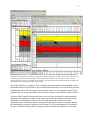
38
Figure 30. The HTML Alignment Viewer output, showing areas where the alignment is not consistent with
structure (red and pink areas of Seq7).
So clearly, this alignment is not perfect, and it needs some enhancement based on what is
isosterically acceptable in 3D and what is not (the score of this alignment based on the formula
described in section 3.2 above is 87). The sequence that is the cause of the problem is also
clearly identified (Seq7). To fix the alignment, we need to edit it in a sequence editor or text
editor where nucleotides can be moved by hand (an automatic aligner based on Stochastic
Context Free Grammar/Markov Random Fields or SCFG/MRF is in preparation; Mokdad, A.,
Sarver, M., Stombaugh, J., Zirbel, C., Leontis, N.B.). Ribostral also provides some insight on
how the alignment should be fixed through its "_Cov.html" output files (where a substitution
table for each BP position is provided with isosterically inspired colored). In this particular case,
and because of the specific BP interactions formed in this motif, a small manipulation of Seq7
second part (after the dots) creates an insertion, but fixes problems with forbidden and
39
heterosteric BPs. After this manipulation, the resulting alignment was viewed again with the
HTML Alignment Viewer, and Figure 31 shows the results:
Figure 31. The corrected alignment as seen again with the Alignment Viewer.
Obviously, Figure 31 shows an improvement in the alignment (new score = 96), eventhough it
created an insertion in Seq7. The manipulation also created an addition gap on the far right of
Seq7, but this may not be a true gap because depending on the unseen nucleotides that are
present beyond this motif (remember, for simplicity the alignment in this example is just an
small extract from a bigger alignment). The reason the alignment was enhanced to this degree is
the fact that the CUG- at the end of Seq7 fit better the isostericity rules of the tSH, tWH, tHS, and
cWW BPs they now occupy (respectively), as compared to the GCUG.
40
References:
1. Hall, T.A. (1999) BioEdit: a user-friendly biological sequence alignment editor and analysis
program for Windows 95/98/NT. Nucl. Acids. Symp. Ser., 41, 95-98.
2. Leontis, N.B. and Westhof, E. (2001) Geometric nomenclature and classification of RNA base
pairs. RNA, 7, 499-512.
3. Jossinet, F. and Westhof, E. (2005) Sequence to Structure (S2S): display, manipulate and
interconnect RNA data from sequence to structure. Bioinformatics, 21, 3320-3321.
4. Leontis, N.B., Stombaugh, J. and Westhof, E. (2002) The non-Watson-Crick base pairs and
their associated isostericity matrices. Nucleic Acids Res, 30, 3497-3531.
5. Lemieux, S. and Major, F. (2002) RNA canonical and non-canonical base pairing types: a
recognition method and complete repertoire. Nucleic Acids Res, 30, 4250-4263.
6. Mokdad, A., Krasovska, M.V., Sponer, J. and Leontis, N.B. (2006) Structural and
evolutionary classification of G/U wobble basepairs in the ribosome. Nucleic Acids Res, 34,
1326-1341.
7. Sarver M., Zirbel C., Stombaugh J., Mokdad A., Leontis N. (2006). Finding Local and
Composite Recurrent Structural Motifs in RNA 3D Structure. Journal of Mathematical Biology
(accepted into special RNA issue).
Citation:
Please cite the following work if you use any component of Ribostral or the nomenclatures
proposed in it:
Mokdad, A., and Leontis, N. (2006). Ribostral: An RNA 3D alignment analyzer and viewer
based on basepair isostericities. Bioinformatics, 22(17): 2168-70.