1
User Manual :
Gegenees
V 1.0.1
What is Gegenees? .................................................................................................................................. 1
Version system: ....................................................................................................................................... 2
What's new .............................................................................................................................................. 2
Installation: .............................................................................................................................................. 2
Perspectives............................................................................................................................................. 3
The workspace......................................................................................................................................... 3
The local database ................................................................................................................................... 4
Remote Sites............................................................................................................................................ 5
Gegenees genome format ....................................................................................................................... 6
Gegenees comparison ............................................................................................................................. 6
Gegenees alignment ................................................................................................................................ 6
Primer alignment ..................................................................................................................................... 7
Analysis .................................................................................................................................................... 7
Group settings tab ................................................................................................................................... 8
Heat plot tab............................................................................................................................................ 9
Score overview tab ................................................................................................................................ 10
Viewing a signature in Artemis.............................................................................................................. 12
Score table tab....................................................................................................................................... 13
Primer alignment/Primer score table tab ............................................................................................. 15
What is Gegenees?
Gegenees is a software that compares genome sequences (Draft and Completed). It was primarily
developed for bacterial genomes but it is also possible to use on viruses and smaller eukaryotes.
Gegenees fragments the genomes and compares all pieces against all genomes. Based on this allagainst-all comparison, a phylogenetic data can be extracted. It is also possible to define a "target
group" and search for genomic regions that have high specificity for the target group. This is referred
to as a "genomic signature". The genomic signature regions can be used to find candidate regions for
the design of primers and probes for ne highly specific diagnostic assays. There is also a built in
primer/probe verification system that compares new candidate or existing primers and probes to the
genomic database and to the defined target groups. Future versions will include more aspects of
comparing next generation sequencing (NGS) data .
Version system:
The first released version was 1.0.1. Based on user feedback, new versions will be released that
solves problems and makes the program easier to use. These versions will be called 1.0.1, 1.0.2 ....
New functionality will lead to version 1.1.1, 1.2.1 ....
To see your version, select "About Gegenees" in the Help main menu.
What's new
This is the first official user manual.
Installation:
The software can be downloaded from http://www.gegenees.org. There are several variants
uploaded, depending on your operating system (OS). Windows. Macintosh and linux are supported.
You must also chose the correct processor architecture (32 bit or 64 bit).
To see the architecture :
In Windows 7 , select "properties" when right clicking "computer".
In Macintosh, select " About this Mac" from the Apple menu. Mac OS X 10.5 (or greater) is a 64-bit.
In Linux, in a terminal, type "uname -a". If "x86_64" or "ia64" is shown, the system is 64 bit.
Java needs to be installed . You may check your Java version at this link:
http://java.com/en/download/installed.jsp.
Download and extract the compressed Gegenees program. Run the Gegenees program from in the
"Gegenes" folder. You will then be asked to specify a "Workspace". This is the place where all your
genomes and comparisons will be stored. In the current version the workspace directory name
SHOULD NOT CONTAIN SPACES. Neither should any of the directories "above" contain spaces. This is
because the BLAST program uses spaces to separate command arguments. A version that is
compatible with spaces is under development, but at this stage spaces should be avoided.
If Gegenees starts OK, it is time to install BLAST. BLAST can be downloaded from
ftp://ftp.ncbi.nih.gov/blast/executables
Gegenees can use both BLAST and BLAST+. In general, The latest version of BLAST+ is recommended.
ftp://ftp.ncbi.nlm.nih.gov/blast/executables/blast+/LATEST
Chose a version that corresponds to your OS and architecture (32 bit/64 bit) and extract (or in
windows run the installation program). In the current version, the directory blast is installed should
NOT CONTAIN SPACES. This requirement will be removed in future versions.
Gegenees must then be configured to find BLAST. Chose "preferences" from Gegenees main menu.
Select blastall for older version of NCBI blast, 2.2.20 and older, and BLAST+ for newer (2.2.21 and
later). If BLAST is added to your system path, you may not need to specify the path. If BLAST is not in
the system path or if BLAST cannot be found by gegenees, specify the full pathname to the directory
containing the BLAST executables.
e.g. Windows, C:\blast\
Linux, \usr\local \blast\
A function for testing if Gegenees finds blast is under implementation and will come in the next
version.
Perspectives
Gegenees have five "perspectives". The active perspective can be changed in the "perspective bar"
just under the main menu. The perspectives are:
Workbench overview :
An overview of all comparisons collected in this "workspace" (se below).
Genomes:
An overview of the genomes available in the local database. Remote
genomes at the NCBI ftp server can also be explored and downloaded.
Genomes can also be copied into a the current comparison.
Alignment:
This is the perspective where the comparative calculations are started
and controlled.
Analysis:
a perspective for phylogenomic and signature analysis of a completed
alignment.
The workspace
The workspace is where all your genomes and your comparison projects will be stored. A wokspace
must always be selected, so when Gegenees starts, the first time a workspace location is asked for.
Typically, a user always use the same workspace. Different users, on the same computer might want
to collect their genomes and comparison in an own, separate workspace. The workspace can be
changed by pressing the "Change workspace" button. Do not use space characters in the workspace
path. The full path of the workspace can be seen in the textbox "Active workspace". The name of the
current workspace can always be seen at the bottom left side of the "status line". The comparisons
that are present in the current workspace will be listed in the table in the Workbench overview
perspective.
The local database
This is where you store your genomes. A "default" database is always present but customized
databases can also be made. The default database represents a directory called "database" in the
workspace. Custom databases represent directories named "database_NameOfCustomDatabase".
The local database content is shown in the middle part of the "Genomes perspective". If the
database is large, subsets can be shown by entering a case sensitive filter text. (e.g Bacillus to show
only the genus Bacillus). There is also a filter for showing only sequences in draft or complete form.
Below is a toolbar with functions for:
•
•
•
•
•
refreshing database content from disk (if you make a manual import of genomes)
Starting an import Wizard.
Selecting all visible genomes (with the current filter)
Deleting selected genomes.
Bring up an information box about the selected genomes (size, GC content, nr contigs etc).
•
•
•
•
Copy genomes, i.e. put genomes in an (Gegenees specific) clipboard.
Paste genomes from the (Gegenees specific) clipboard.
Change name or type (complete/Draft) for a genome
copy to the current comparison (genomes can also be copied from a comparison into the
local database if needed, e.g. if you get a ready-made comparison)
Remote Sites
It is possible to download genomes from a remote FTP server. The FTP-sites are definend by a file
ending with ".site" in the "ftp" directory in the workspace directory. A few pre-defined ftp sites are
distributed with the Gegenees software. These are NCBI complete genomes (pointing at
ftp://ftp.ncbi.nih.gov/genomes/Bacteria/) and NCBI genomes bacteria draft (pointing at
ftp://ftp.ncbi.nih.gov/genomes/Bacteria_DRAFT/) and NCBI genbank bacteria draft (pointing at
ftp://ftp.ncbi.nih.gov/genbank/wgs/) "NCBI genbank bacteria draft" contains more genomes than
"NCBI genomes bacteria draft". It is possible to make own ".site" files. Copy the content of the
existing files and replace the "HostName:" and the "Directory:" fields with custom information. The
FTP site must be formatted as the NCBI site. If you need to connect to other types of ftp sites,contact
the support at Gegenees.
Gegenees genome format
Gegenees uses a folder for each genome. The folder name corresponds to the Name of the genome
as appearing in Gegenees and the type of the genome ("Draft"/"Complete". The last part of the
folder name has the format "--Draft--" or "--Complete". In future versions, more types may be
introduced. The folder contains at least one Genbank formatted file with extension ".gbk" or ".gbff".
If there are several subsequences/contigs, they may be in the same file or in separate files. Genomes
are stored in the database folder(s) but also in the comparison folders. Thus. the comparison keeps a
copy of the part of the database it is using. If the database is modified, the genomes belonging to a
comparison is still untouched in the comparison folder.
Gegenees comparison
The Gegenees "comparison" is a "package" containing:
•
•
•
•
a list of genomes that belongs to the comparison
a copy of all the genomes as they looked like when they were added to the comparison
typically, at least one "alignment" which represents a comparative calculation at a certain
resolution (se below).
Files coupled to the analysis of the alignment (s).
Thus, the first step when making an comparative analysis is to define the genomes. This can be done
by copying the from the "local database" part in the "Genomes" perspective into the "current
comparison" in the right part of the "Genomes" perspective. This is typically done with the "green
arrow". The list of genomes and the genome copies are then produced. No alignment is created at
this time. A comparison is represented by a folder with the prefix "comparison_" and it contains
copies of the genomes and a file "comparison.geg" that contains the genome list.
Gegenees alignment
When a comparison is defined, one or several alignments can be made. The alignment represents a
comparative calculation thatn be made at different resolutions. An alignment is created in the
"Alignment" perspective with the "New..." button. Two type of alignments can be made,
"fragmented alignment" and "primer alignment". the primer alignment is a special case and is
described below in a separate heading. The resolution of the alignment is controlled by two
parameters, the "fragment size" and the "sliding step size". The fragment size represents the
"scanning window size" and it should be smaller than the genomic region you anticipate to find in
the analysis. For bacteria, we recommend 200 frag-size/100 slide-size (more accurate) and 500/500
(much faster and usually sufficient)settings. Small fragment sizes and sliding step sizes gives more
demanding calculations. When working with viruses and small sequences, shorter settings may be
needed. It is also possible to use tblastx (compares sequences on translated level, i.e aminocids). This
is very much more demanding and the datasets should be smaller. If the sequences are
pylogenetically far apart, this may be a useful operating mode. An alignment is represented on the
disc by a folder with the prefix "alignment_".
When an alignment is defined it can be started by pressing the "start" button. The calculation
progress will be shown and the log-window in the right part will show messages on what is
happening. Typically, first a lot of conversion and preparation messages appears. Then the a BLAST
list is created and executed in parallel "threads". Typically, each "thread" should not take more than
at the most a few minutes to complete. The number of simultaneously calculating threads is
indicated and also the thread number and the total number of threads that should be run. It is
possible to send a pause signal and then resume the calculation later. After all the threads have been
run, some data analysis is made and then the alignment is completed. Once a alignment is
completed, it is possible to analyze the data in the "Analysis" perspective. There is an export button
after the "Nr of genomes" field that can be used to export a list of accession numbers for the
genomes.
Primer alignment
Primer alignments is a special type of alignment where primers and/or probes are used instead of
fragments. This is usually not as demanding calculation as fragmented alignments. The primer
alignment is analyzed in a special tab in the analysis perspective (see below).
Analysis
The analysis perspective contains different tools for analyzing the data from a completed alignment.
The tabs are:
Group settings:
A tabular view of the genomes that allows definition of the target and
background groups for the analysis.
Heat plot:
This tab represents an phylogenomic overview of the data based on average
similarities.
Score overview:
This tab represents a graphical overview and exploration tool of the genomic
regions that are unique or discriminatory for the target group.
Score table:
This tab represents a tabular exploration tool for the genomic regions that
are unique or discriminatory for the target group.
Primer score table:
This tab allows analysis of "primer alignments" to compare specificity of
primers and probes based on the genomic data and the target group settings.
Group settings tab
The group settings tab allows the target group and the background group to be define.
•
•
•
•
The target group represents the genomes that you are interested in. You might want to find
discriminatory genomic regions that can be used to design specific molecular assays. You
might also be interested in finding and analyzing genomic regions that are associated with a
specific phenotypic trait that the target group share. The target group should ideally contain
genomes that represents the genomic variability in the group as well as possible.
The background group represents other genomes. The background should contain the
genomes that are most likely to give a cross-reaction (false positive in an assay). For best
result, close neighbor strains/isolates that do not contain the phenotypic trait should be
included.
Excluded genomes. You may also chose to exclude genomes from the analysis.
The reference genome is the genome where the nucleotide coordinate system and the
annotations are collected from. For a high stringency biomarker analysis (se below), the best
annotated genome in the target group should be used. For lower stringencies in the
biomarker analysis, the result may be slightly different depending on which target genome is
selected as reference. It is then good to look at the data with different reference genomes. A
reference genome must be chosen to be able to look at the score overview and score table
tabs.
Several group settings can be created from the same dataset (e.g. different subtypes) with the
"New.." or "Make a copy..." buttons.
Heat plot tab
The heat plot tab gives an phylogenomic overview of the data. shown. The average normalized
BLAST score values of all fragments are shown. It is also possible to define threshold values, meaning
that that fragments falling under the threshold is not used to calculate the average similarity value.
This gives a better phylogenetic signal since the similarity value is only based on conserved genetic
material (the core genome). It is also possible to see how large the core genome is at the specified
threshold (select "show core" insted of "show score"). It is possible to change the "color profile" of
the heatplot so that differences are highlighted as well as possible for the particular dataset. The
number of decimals shown can be changed. The genomes are sorted alphabetically, which often is
sufficient. There are sorting possibilities built in for the heat plots. It is possible to move genomes or
group of genomes with the "Move selection to row" field or by right clicking it and select "move"
from the context menu. The target and background group settings can also be modified from the
right click-context menu. If, "Drag and drop, single sorting" is selected, genomes can be draged with
the mouse, one by one. The sort is saved and if several sorts are wanted, new ones can be created
with the "new..." button. There is also an "autosort" function, that tries to minimize the distances
between the rows. There is also an export button that allows of the phylogenomic data:
•
•
•
export of the table in tab-format (for work in spreadsheet programs)
export as html. Can be opened in a web browser or converted to publication grade figures.
This is sometimes a better overview if the table is very large.
export nexus file. Use this export to create dendrograms in e.g. SplitsTree .
Score overview tab
The score overview tab shows a graphic representation of the "biomarker scores". biomarker scores
are score values that rank all genomic regions (fragments) in how discriminating they are for the
target group in terms of conservation (no false negatives) and uniqueness (no false positives in the
background). There are three types of scores with different stringencies:
Biomarker score (max/min):
represents the highest stringency. The high scoring fragments
must be present and conserved in ALL target group genomes
and must be absent or very diverged in ALL background
genomes. The score goes from 0 (or negative values)
representing bad regions up to 1 which represents a perfect
region. The score is based on the worst background genome
(max score) and on the worst target group genome (min
score).
Biomarker score (max/average)
Similar to Biomarker score (max/average) but uses average
values of the background group (relaxes the uniqueness
criterion)
Biomarker score (average/average)
Similar to Biomarker score (max/average) but uses average
values of the background group and the target group (relaxes
the uniqueness and the conservation criterion)
Target group maximum score
Shows the best score in the target group (self score). This is
usually 100% everywhere, but if bad regions are present in the
sequence (e.g. nnnnnnnnnnnnnn), they can be identified here.
Target group minimum score
Shows the worst conservation within the target group. Can be
used to find highly conserved regions.
Target group average score
Shows the average conservation within the target group. Can
be used to find highly conserved regions.
Background group maximum score
Shows the best score in the background group. This represent
the worst cross reaction.
Background group minimum score
Shows the minimum score in the background group. Can be
used to find regions that are not conserved in a group of very
related genomes.
Background group average score
Shows the average conservation within the background group.
The biomarker scores are drawn graphically. There is possibilities to compare two types of scores by
drawing one upwards (from the coordinate axis) and a second downwards. The graphical view is
spitted into two rows in order to use the computer screen optimal (do not confuse the upper row
with the upwards score, there are upwards scores in both rows) . there is a possibility to exclude
draft genomes in the calculations since they sometimes lack regions that in some cases may disturb
the analysis. When the mouse moves over the graph, the subsequence,fragment number and
coordinate at the cursor position is shown in the "info" part to the right. The number of fragments
that each pixel column on the screen represent, is also indicated. It is also possible to see how many
percent of the genome has a biomarker score over a certain threshold. This gives a good overview of
the how much genomic regions one can expect.
It is possible to zoom into the graph by selecting a region with the right mouse button down. If the
left mouse button is used, the corresponding region is selected. A selection can thereafter be loaded
into the tabular view for further data mining.
There are possibilities to export the graph (as seen on the screen) as an image. It is also possible to
export the data to a file that can be explored in Artemis (se section below).
Viewing a signature in Artemis
It is possible to export an interesting subsequence from the genome (or the whole genome if it is
completed) into a format that can be viewed in Artemis
http://www.sanger.ac.uk/resources/software/artemis/.
The export will end up in a directory called "export" under the workspace directory. It will be a
"*.gbk" file that essentially is the same file as the original "gbk" file (if there are problems or warnings
when loading the original file in Artemis they will remain). The "gene" and "misc feature" track is
replaced by the biomarker scores. Five files are exported
1.
2.
3.
4.
5.
the original annotated file with also the gene and misc feature track intact.
a file with Biomarker scores (max/min) as a misc_feature track
a file with Biomarker scores (max/avr) as a misc_feature track
a file with Bimarker scores (avr/avr) as a misc_feature track
a file with Biomarker scores (max/min), only complete genomes as a misc_feature track
an example of how this kind of export will look like in artemis is shown below.
Score table tab
In the "score table" tab, details about the fragments representing either
•
•
•
•
a selection (e.g. a range defined by the mouse in the graphical view)
a user defined range (expressed as fragment numbers)
a subset of fragments with a specific biomarker score-range (e.g. 0.8-1.0)
(1.0 is the maximum biomarcer score)
If none of the range boxes are checked, all fragments will be shown
Fragments from a certain subsequence can also be selected. After setting the filtering range (or a
combination of them, e.g. all fragments in the first 200 kb of subsequence 2 with biomarker sore
over 0.8)press the "show fragments" button to load the fragments. It is possible to sort the table
based by clicking the header. The type of biomarker score to be shown can be selected in the info
region.
Show sequence displays the actual sequences of the fragments and it is possible to fuse adjacent and
overlapping fragments into continuous sequences. The sequences can be exported to a Fasta-file or
sent to a web page ready for a blast comparison at NCBI.
The detailed scores, shows how each fragment scores against each genome in the target and
background group. This may help to identify which particular strain is causing a cross reaction.
It is also possible to export the table (as its shown) or the full data table (without filtering) as a tab
delimited text file for further analysis in e.g. a spreadsheet program.
Primer alignment/Primer score table tab
To make a primer/probe analysis, create or use an existing comparison with the genomes of interest.
Create a "primer alignment" and press "set primers". enter your primers and run the analysis.
The primer alignment can now be explored in the "Primer score table tab". The "unalignment" index,
represents missmatches in the alignment plus non-aligned nucleotides. It is marked green if it is a
perfect match. A target group/ background group setting can be loaded from a fragmented
alignment in the same comparison, and the genomes are color coded accordingly, so that a the
primer matching can easily be compared to the target group definition.
If a primer row is double-clicked with the mouse or the "show alignment" button is pressed, the
alignment of this primer against this genome is shown. The table and the alignment views can also be
exported as text files.