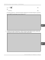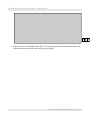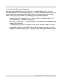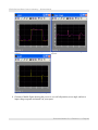
Download Rotary Experiment #04: BB01 Control Ball and Beam Position

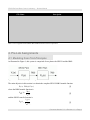
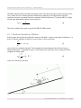
Rotary Motion Servo Plant: SRV02
Rotary Experiment #04:
BB01 Control
Ball and Beam Position Control using
QuaRC
Student Manual
SRV02 Ball and Beam Laboratory – Student Manual
Table of Contents
1. INTRODUCTION..........................................................................................................................................1
2. PREREQUISITES.........................................................................................................................................1
3. OVERVIEW OF FILES..................................................................................................................................2
4. PRE-LAB ASSIGNMENTS.............................................................................................................................4
4.1. Modeling from First-Principles........................................................................................................4
4.1.1. Nonlinear Equation of Motion...............................................................................................................5
4.1.2. Adding SRV02 Dynamics......................................................................................................................8
4.1.3. Obtaining Transfer Function..................................................................................................................9
4.2. Desired Control Response..............................................................................................................11
4.2.1. Time-Domain Specifications................................................................................................................11
4.2.2. Settling Time .......................................................................................................................................11
4.2.3. Percentage Overshoot and Peak Time..................................................................................................13
4.2.4. Steady-state Error.................................................................................................................................13
4.3. Ball and Beam Cascade Control Design.........................................................................................14
4.3.1. Inner Loop Design: SRV02 PV Position Controller.............................................................................15
4.3.2. Outer Loop Stability Analysis..............................................................................................................17
4.3.3. Outer Loop Controller Design..............................................................................................................22
5. IN-LAB PROCEDURES...............................................................................................................................33
5.1. Position Control Simulation...........................................................................................................33
5.1.1. Outer-Loop Simulation........................................................................................................................33
5.1.2. Cascade Control Simulation.................................................................................................................40
5.2. Position Control Implementation....................................................................................................53
5.2.1. Setup for Position Control Implementation..........................................................................................54
5.2.2. Running the Practical PD Controller....................................................................................................54
Document Number 711 ♦ Revision 1.1 ♦ Page i
SRV02 Ball and Beam Laboratory – Student Manual
5.2.3. Controlling using the Remote Sensor (Optional).................................................................................60
6. RESULTS SUMMARY.................................................................................................................................62
7. REFERENCES...........................................................................................................................................63
Document Number 711 ♦ Revision 1.1 ♦ Page ii
SRV02 Ball and Beam Control Laboratory – Student Manual
1. Introduction
The objective of the Ball and Beam experiment is to stabilize the ball to a desired position along the
beam. Using the proportional-derivative (PD) family, a cascade control system is designed to meet a set
of specifications.
The following topics are covered in this laboratory:
● Model the dynamics of the ball from first-principles.
● Obtain a transfer function representation of the system.
● Design a proportional-velocity (PV) compensator to control the position of the servo load shaft
according to certain time-domain requirements.
● Using root locus, assess whether or not the specifications can be met with a certain type of
compensator.
● Design a compensator that regulates the position of the ball on the beam and meets certain
specifications. This together with the servo control is the complete Ball and Beam cascade
control system.
● Simulate the Ball and Beam control using the model of the plant and ensure the specifications
are met without any actuator saturation.
● Implement the controllers on the Quanser BB01 device and evaluate its performance.
2. Prerequisites
In order to successfully carry out this laboratory, the user should be familiar with the following:
● Data acquisition card (e.g. Q8), the power amplifier (e.g. UPM), and the main components of
the SRV02 (e.g. actuator, sensors), as described in References [1], [4], and [5], respectively.
● Wiring and operating procedure of the SRV02 plant with the UPM and DAC device, as
discussed in Reference [5].
● Laboratory described in Reference [6] in order to be familiar using QuaRC with the SRV02.
● Designing a PV position control for the SRV02 as dictated in Reference [8].
Document Number 711 ♦ Revision 1.1 ♦ Page 1
SRV02 Ball and Beam Control Laboratory – Student Manual
3. Overview of Files
Table 1 below lists and describes the various files supplied with the SRV02 Ball and Beam Position
Control laboratory.
File Name
Description
09 – Ball and Beam User
Manual.pdf
This manual describes the hardware of the Ball and Beam and
explains how to setup and wire the system for the experiments.
10 – Ball and Beam Position
Control – Student Manual.pdf
This laboratory guide contains pre-lab and in-lab exercises
demonstrating how to design and implement a position controller
on the Quanser SRV02 Ball and Beam plant using QuaRC.
setup_srv02_exp04_bb01.m
The main Matlab script that sets the SRV02 motor and sensor
parameters, the SRV02 configuration-dependent model parameters,
and the BB01 sensor parameters. Run this file only to setup the
laboratory.
config_srv02.m
Returns the configuration-based SRV02 model specifications Rm,
kt, km, Kg, eta_g, Beq, Jeq, and eta_m, the sensor calibration
constants K_POT, K_ENC, and K_TACH, and the UPM limits
VMAX_UPM and IMAX_UPM.
config_bb01.m
Returns the configuration-based BB01 model specifications
L_beam, r_arm, r_b, m_b, J_b, and g, the servo offset
THETA_OFF, the min/max servo limits THETA_MIN and
THETA_MAX, and the sensor calibration constant K_BS.
d_model_param.m
Calculates the SRV02 model parameters K and tau based on the
device specifications Rm, kt, km, Kg, eta_g, Beq, Jeq, and eta_m.
calc_conversion_constants.m
Returns various conversions factors.
s_bb01_pos_outer_loop.mdl
Simulink file that simulates the closed-loop system when using
only the outer-loop ball position controller with the BB01 system,
i.e. no inner loop control of the servo position.
s_bb01_pos.mdl
Simulink file that simulates the cascade ball position controller.
Both the outer-loop ball position control and the inner-loop servo
position control are used in this file.
q_bb01_pos.mdl
Simulink file that implements a closed-loop cascade position
controller on the actual BB01 system using QuaRC.
Document Number 711 ♦ Revision 1.1 ♦ Page 2
SRV02 Ball and Beam Control Laboratory – Student Manual
File Name
Description
Document Number 711 ♦ Revision 1.1 ♦ Page 3
SRV02 Ball and Beam Control Laboratory – Student Manual
File Name
Description
Table 1: Files supplied with the SRV02 Ball and Beam Position Control experiment.
4. Pre-Lab Assignments
4.1. Modeling from First-Principles
As illustrated in Figure 1, this system is comprised of two plants: the SRV02 and the BB01.
Figure 1: Ball and Beam open-loop block diagram.
The main objective in this section is to obtain the complete SRV02+BB01 transfer function
P( s ) = Pbb( s ) Ps( s )
[1]
where the BB01 transfer function is
X( s )
Pbb( s ) =
[2]
Θ l( s )
and the SRV02 transfer function is
Θ l( s )
Ps( s ) =
[3]
Vm ( s )
.
Document Number 711 ♦ Revision 1.1 ♦ Page 4
SRV02 Ball and Beam Control Laboratory – Student Manual
The BB01 transfer function describes the displacement of the ball with respect to the load angle of the
servo. In the next few sections, the time-based motion equations are developed and, from these
equations of motion, its transfer function is obtained. Recall in Reference [7], that the SRV02 voltageto-load angle plant transfer function was found to be
K
Ps( s ) =
[4]
(τ s + 1) s .
This can be added to the system to get the full SRV02+BB01 model.
4.1.1. Nonlinear Equation of Motion
In this section, the equation describing the motions of the ball, x, relative to the angle of the beam, α, is
derived. Thus the equation of motion, or eom for short, will be of the form
2
d
x( t ) = f( α ( t ) )
[5]
2
dt
,
where f(α(t)) is a nonlinear function. The incomplete free-body diagram of the ball on a beam is
illustrated in Figure 2. Applying Newton's Law of Motion, the sum of the forces acting on the ball
alongside the beam equals
 2

d

mb 
x( t )  =
F
[6]
 2

 dt

,
where mb is the mass of the ball.
∑
Figure 2: Free-body diagram of Ball and Beam.
Document Number 711 ♦ Revision 1.1 ♦ Page 5
SRV02 Ball and Beam Control Laboratory – Student Manual
Neglecting friction and viscous damping, the ball forces can can be represented by
 2

d


mb
x( t )  = Fx , t − Fx , r
[7]
 2

 dt

,
where Fr is the force from the ball's inertia and Ft is the translational force generated by gravity. For the
ball to be stationary at a certain moment, i.e. be in equilibrium, the force from the ball's momentum
must be equivalent to the force produced by gravity.
1. Find the force in the x direction (along the beam) that is caused by gravity, Fx,t.
0 1 2
2. Find the force that is caused by rotational inertia of the ball in the x direction, Fx,r.
Hint: Use the sector formula to convert between linear and angular displacement (e.g. or
velocity and acceleration)
x( t ) = γ b( t ) rb
[8]
where γb is the angle of the ball and rb is the ball radius.
Document Number 711 ♦ Revision 1.1 ♦ Page 6
SRV02 Ball and Beam Control Laboratory – Student Manual
0 1 2
3. Give the nonlinear equation of motion of the ball and beam. It should be in the form shown in
[5].
0 1 2
4.1.2. Adding SRV02 Dynamics
In this section the equation of motion representing the position of the ball relative the angle of the
Document Number 711 ♦ Revision 1.1 ♦ Page 7
SRV02 Ball and Beam Control Laboratory – Student Manual
SRV02 load gear is found. The obtained equation is nonlinear (includes a trigonometric term) and it
will have to be linearized in order for the model to be used for control design.
1. Using the schematic given in Reference [9], find the relationship between the SRV02 load gear
angle, θl, and the beam angle, α.
0 1 2
2. Find the equation of motion that represent the ball's motion with respect to the SRV02 angle θl.
Linearize the equation of motion about servo angle θl(t) = 0
0 1 2
3. Simplify the expression by lumping the coefficient parameters of θl(t) into parameter Kbb. This
is the model gain of the Ball and Beam system. Show the new simplified equation of motion.
Document Number 711 ♦ Revision 1.1 ♦ Page 8
SRV02 Ball and Beam Control Laboratory – Student Manual
Then, evaluate the model gain numerically using the Ball and Beam parameters given in
Reference [9].
Hint: Recall that the moment of inertia of a solid sphere is
2
2mr
[9]
J=
5
where m is the mass of the ball and r is its radius.
0 1 2
4.1.3. Obtaining Transfer Function
In this section the transfer function describing the servo voltage to ball position displacement is found.
1. Find the transfer function Pbb(s) of the BB01. Assume all initial conditions are zero.
Document Number 711 ♦ Revision 1.1 ♦ Page 9
SRV02 Ball and Beam Control Laboratory – Student Manual
0 1 2
2. Give the complete SRV02+BB01 process transfer function P(s).
0 1 2
Document Number 711 ♦ Revision 1.1 ♦ Page 10
SRV02 Ball and Beam Control Laboratory – Student Manual
4.2. Desired Control Response
4.2.1. Time-Domain Specifications
The time-domain specifications for controlling the position of the SRV02 load shaft are:
ess = 0
[10]
,
t p = 0.15 [ s ]
[11]
, and
PO = 5.0 [ "%"] .
[12]
Thus when tracking the load shaft step reference, the transient response should have a peak time less
than or equal to 0.15 seconds, an overshoot less than or equal to 5 %, and no steady-state error.
The specifications for controlling the position of the ball are:
ess ≤ 0.005 [ m ]
,
t s = 3.5 [ s ]
cts = 0.04
, and
PO = 10.0 [ "%"] .
[13]
[14]
[15]
[16]
Given a step reference, the peak position of the ball should not overshoot over 10%. After 3.5 seconds,
the ball should settled within 4% of its steady-state value (i.e. not the reference) and the steady-state
should be within 5 mm of the desired position.
4.2.2. Settling Time
The response of a second-order system, y(t), when subjected to a unit step reference, r(t), is shown in
Figure 3. This response has a 5% settling time of 0.30 seconds. Thus the response settles within 5% of
its steady-state value, which is between 0.95 and 1.05, in 0.30 seconds. Settling time is defined
ts = t1 − t0
[17]
where the initial step time is t0 and the time it takes to settle is t1.
Document Number 711 ♦ Revision 1.1 ♦ Page 11
SRV02 Ball and Beam Control Laboratory – Student Manual
Figure 3: Settling time of unit step response.
An equation that expresses the settling time in terms of the natural frequency, ωn, and the damping of a
second-order system, ζ, is required. In order to find this, an exponentially decreasing sinusoidal is used
to approximate the upper-bound of the response and is expressed
( − ζ ω n ts )
e
[18]
yub = 1 +
2
1− ζ
.
1. Given the settling time percentage equation
cts = yub − 1
[19]
and the upper-bound formula, show that the settling time equation is
2
ln( cts 1 − ζ )
ts = −
ζ ωn
.
[20]
Document Number 711 ♦ Revision 1.1 ♦ Page 12
SRV02 Ball and Beam Control Laboratory – Student Manual
0 1 2
4.2.3. Percentage Overshoot and Peak Time
Recall from Reference [8] that the peak time and percentage overshoot equations are
π
tp =
[21]
2
ωn 1− ζ
and
PO = 100 e

−



π ζ


2 
1− ζ 
[22]
.
4.2.4. Steady-state Error
In this section, the steady-state error of the ball position is evaluated using a proportional compensator.
Recall the unity feedback system in Figure 4.
Figure 4: Unity feedback system.
Document Number 711 ♦ Revision 1.1 ♦ Page 13
SRV02 Ball and Beam Control Laboratory – Student Manual
1. Find the steady-state error the ball and beam, Pbb(s), with a unity compensator
C( s ) = 1
[23]
and a reference step of
R0
[24]
R( s ) =
s ,
where R0 is the step amplitude. Remark that in this calculation the SRV02 dynamics are ignored
and only the BB01 plant is being considered. If there is no constant steady-state error, then
describe the error of the system.
0 1 2
4.3. Ball and Beam Cascade Control
Design
The cascade control that will used for the SRV02+BB01 system is illustrated by the block diagram
given in Figure 5. Based on the measured ball position X(s), the ball and beam compensator, Cbb(s), in
the outer-loop computes the servo load angle needed, Θd(s), to attain the desired ball position, Xd(s).
The inner loop is a servo position control system as described in Reference [8]. Thus the servo
compensator Cs(s) calculates the motor voltage required for the load angle to track the given desired
load angle.
Document Number 711 ♦ Revision 1.1 ♦ Page 14
SRV02 Ball and Beam Control Laboratory – Student Manual
Figure 5: Cascade control system used to control ball position in SRV02+BB01 plant.
In Section 4.3.1, the position controller for the SRV02 is designed, similarly as explained in Reference
[8]. A compensator is introduced in Section 4.3.2 and it is assessed using root locus whether it can be
used to meet the desired specifications. Two different variations of a compensator are designed in
Section 4.3.3.
4.3.1. Inner Loop Design: SRV02 PV Position Controller
In this section, the proportional-velocity (PV) controller gains are computed for the SRV02 when it is
in the high-gear configuration and based on the specifications given in Section 4.2.1. The internal
control loop is depicted in the block diagram shown in Figure 6.
Figure 6: SRV02 closed-loop system.
1. The nominal model parameters, K and τ, when the SRV02 is in high-gear configuration are
Document Number 711 ♦ Revision 1.1 ♦ Page 15
SRV02 Ball and Beam Control Laboratory – Student Manual
 rad 

K = 1.76 
 sV 
and
τ = 0.0285 [ s ] .
[25]
[26]
Given these parameters, calculate the minimum damping ratio and natural frequency required to
meet the SRV02 specifications given in Section 4.2.1.
0 1 2
2. Using the derivations in Experiment #2: SRV02 Position Control (Reference[8]), calculate the
control gains needed to satisfy the time-domain response requirements.
0 1 2
Document Number 711 ♦ Revision 1.1 ♦ Page 16
SRV02 Ball and Beam Control Laboratory – Student Manual
4.3.2. Outer Loop Stability Analysis
The inner loop that controls the position of the SRV02 load shaft is complete and it the servo dynamics
are now considered negligible. Thus it is assumed that the desired load angle equals the actual load
angle
θ l( t ) = θ d( t )
[27]
.
The outer-loop shown in Figure 7 will be used to control the position of the ball on the beam.
Figure 7: BB01 closed-loop system.
4.3.2.1. Root Locus of Open-Loop System
The root locus shows how the poles of a closed-loop system move when a proportional gain increases
towards infinity.
1. Using Figure 7, find the closed-loop transfer function of the BB01 system with the proportional
control
Cbb( s ) = Kc
[28]
.
Document Number 711 ♦ Revision 1.1 ♦ Page 17
SRV02 Ball and Beam Control Laboratory – Student Manual
0 1 2
2. Plot the root locus of the BB01 plant Pbb(s). The closed-loop transfer function found above can
help describe how the poles behave as Kc goes to infinity.
Document Number 711 ♦ Revision 1.1 ♦ Page 18
SRV02 Ball and Beam Control Laboratory – Student Manual
0 1 2
4.3.2.2. Desired Location of Poles
Consider the prototype second-order system
ω n2
Y( s )
=
R( s )
2
s + 2 ζ ω n s + ω n2
[29]
.
The location of the two poles of this system when the natural frequency is
Document Number 711 ♦ Revision 1.1 ♦ Page 19
SRV02 Ball and Beam Control Laboratory – Student Manual
 rad 

ω n = 1.5 
 s 
and the damping ratio is
ζ = 0.6
is illustrated in Figure 8.
[30]
[31]
Figure 8: Desired pole locations.
As illustrated, the natural frequency determines the radial length of the poles from the origin. The
damping ratio changes the angle where they are positioned from the imaginary axis according to the
relationship
θ = arcsin( ζ ) .
[32]
The location of the poles along the imaginary axis is called the damped natural frequency
2
[33]
ωd= ωn 1− ζ
,
and the position of the poles along the real-axis is described by the equation
σ = ζ ωn
[34]
.
Document Number 711 ♦ Revision 1.1 ♦ Page 20
SRV02 Ball and Beam Control Laboratory – Student Manual
1. Find the natural frequency and damping ratio required to achieve the time-domain specifications
of the Ball and Beam plant given in Section 4.2.1.
0 1 2
2. Similarly as shown in Figure 8, plot the region where the poles should lie to satisfy the
specifications.
0 1 2
3. Discuss the response if the poles lie beyond the radius circle along the diagonal lines, i.e. away
from the imaginary axis. Also, comment on what happens if the poles of the system lie inside
the diagonal lines along the radius circle, i.e. moving towards the real axis. Make references to
its effects on the settling time and overshoot of the response.
Document Number 711 ♦ Revision 1.1 ♦ Page 21
SRV02 Ball and Beam Control Laboratory – Student Manual
0 1 2
4. Based on the root locus obtained previously, can the specifications of the Ball and Beam system
be satisfied using a proportional controller? Discuss.
0 1 2
4.3.3. Outer Loop Controller Design
So far the analysis has been done using a proportional compensator. Now the affects using a dynamic
compensator in the loop path of Figure 7 is studied. Generally speaking, adding a zero in the forwardpath increases the bandwidth of the closed-loop system. Adding a pole increases the rise time and
overshoot of the system but makes it overall less stable. In our case, the bandwidth must be increased
and the overshoot has to be minimized.
The effects of adding a zero in the forward loop path are studied Section 4.3.3.1 and the obtained
steady-state error is assessed in Section 4.3.3.2. The first controller to be designed is a proportionalderivative (PD) compensator. This is done in Section 4.3.3.3. This design is then modified in Section
Document Number 711 ♦ Revision 1.1 ♦ Page 22
SRV02 Ball and Beam Control Laboratory – Student Manual
4.3.3.4 to handle some inherent practical issues.
4.3.3.1. PD Compensator Analysis
Consider the following PD compensator
Cbb( s ) = Kc ( s + z )
,
where Kc is the proportional gain and z is the location of the compensator zero.
[35]
1. Plot the root locus of the BB01 loop transfer function
Lbb( s ) = Cbb( s ) Pbb( s )
[36]
when the compensator zero is placed somewhere between 0.2 and 0.5 along the negative real
axis.
0 1 2
Document Number 711 ♦ Revision 1.1 ♦ Page 23
SRV02 Ball and Beam Control Laboratory – Student Manual
2. Could this compensator be used to satisfy the ball and beam settling time and overshoot
specifications? Explain with references to the location of the zero and the gain.
0 1 2
3. Find the closed-loop transfer function of the ball and beam, X(s)/Xd(s), when using the
proportional-velocity (PV) controller shown in Figure 9. This is a variation of the PD
compensator that does not feed the setpoint velocity, sXd(s), and is similar to what is used to
control the position of the SRV02.
Figure 9: Ball and beam ideal PV controller.
Document Number 711 ♦ Revision 1.1 ♦ Page 24
SRV02 Ball and Beam Control Laboratory – Student Manual
0 1 2
4.3.3.2. Steady-State Error
In this section, it is assessed whether the steady-state error specification, given in [13], can be met using
the PD controller in [35].
1. Find the BB01 error transfer function when using PD compensator [35]. Can the final-value
theorem be used on this system?
0 1 2
Document Number 711 ♦ Revision 1.1 ♦ Page 25
SRV02 Ball and Beam Control Laboratory – Student Manual
2. Find the steady-state error of the BB01 closed-loop system with the PD controller. Can the
steady-state error requirement in [13] be satisfied using a PD compensator?
0 1 2
4.3.3.3. Ideal PD Control Design
The proportional and velocity gains needed to meet the desired requirements in Section 4.2.1 are found
in this section. This is called the ideal PD controller.
1. Where should the zero lie and the gain be to meet the settling time and overshoot
specifications? Find expressions for the zero location, z, and the compensator gain, Kc, that will
satisfy a given natural frequency and damping ratio.
Document Number 711 ♦ Revision 1.1 ♦ Page 26
SRV02 Ball and Beam Control Laboratory – Student Manual
0 1 2
2. Based on the expressions found, evaluate numerically the zero location and gain needed to
satisfy the specifications.
0 1 2
4.3.3.4. Practical PD Controller
The designed ideal PD controller cannot be used to control the ball position on the actual BB01 device
because it takes a direct derivative to obtain the ball velocity. The position of the ball is measured using
an analog sensor and it has some inherent noise. Taking the derivative of this type of signal would
Document Number 711 ♦ Revision 1.1 ♦ Page 27
SRV02 Ball and Beam Control Laboratory – Student Manual
output results in an amplified high-frequency signal that is eventually fed back into the motor and
causes a grinding noise. As illustrated by H(s) in Figure 10, this is prevented by using a high-pass filter.
The first-order filter replaces the derivative in Figure 10 and has the form
ωfs
H( s ) =
[37]
s+ ωf
.
For adequate filtering of the noise found in the BB01 linear transducer, the cutoff frequency will be set
to 1 Hz, or
 rad 

ω f = 6.28 
[38]
 s  .
Also added to the controller is the set-point weight parameter bsp. This varies the amount of setpoint
that is used to compute the error velocity. This compensator is called the practical PD controller.
Figure 10: BB01 PD controller with filtering.
Although filtering is often necessary when controlling actual systems to make it more robust against
noise, it does add dynamics to the system. Thus the compensator gain and zero location have to be
recomputed in order to meet the specifications listed in Section 4.2.1.
1. Using the block diagram in Figure 10, find the closed-loop equation of the BB01 (only the
outer-loop, no servo dynamics).
Document Number 711 ♦ Revision 1.1 ♦ Page 28
SRV02 Ball and Beam Control Laboratory – Student Manual
0 1 2
2. Find the BB01 compensator, Cpp(s) in Figure 7, when the set-point weight of the practical PD
controller is 1, i.e. bsp = 1.
0 1 2
3. Find the locations of the zero and the pole of the compensator. What type of compensator does
the PD becomes when adding filtering (e.g. lead or lag)?
Document Number 711 ♦ Revision 1.1 ♦ Page 29
SRV02 Ball and Beam Control Laboratory – Student Manual
0 1 2
4. The third-order characteristic equation is
2
[38]
( s + 2 ζ ω n s + ω n 2 ) ( 1 + Tp s )
where Tp is the pole decay in seconds. Where should the zero and pole lie and the gain be to
meet the settling time and overshoot specifications? First, find an expressions for the pole
location, Tp, that will satisfy the natural frequency and damping ratio requirements in Section
4.2.1 as well as the desired filter cutoff frequency given in [38].
Document Number 711 ♦ Revision 1.1 ♦ Page 30
SRV02 Ball and Beam Control Laboratory – Student Manual
0 1 2
5. Find expressions for the zero location, z, and the compensator gain, Kc, that will satisfy ωn and ζ
in Section 4.2.1 and the desired filter cutoff frequency in [38].
Document Number 711 ♦ Revision 1.1 ♦ Page 31
SRV02 Ball and Beam Control Laboratory – Student Manual
0 1 2
6. Based on the expressions found, evaluate numerically the pole time constant, zero location, and
gain needed to satisfy the specifications.
0 1 2
Document Number 711 ♦ Revision 1.1 ♦ Page 32
SRV02 Ball and Beam Control Laboratory – Student Manual
5. In-Lab Procedures
The closed-loop response of the Ball and Beam is simulated in Section 5.1 and then implement on the
actual BB01 device in Section 5.2.
5.1. Position Control Simulation
Go through Section 5.1.1 to simulate the Ball and Beam system using the designed compensator and
ensure it meets the specifications listed in Section 4.2.1. This section deals with only the outer-loop
control. In Section 5.1.2, the ball and beam is simulated using its full cascade control system. That is,
the system that includes both the outer ball position control loop and the inner servo position control
feedback loop.
5.1.1. Outer-Loop Simulation
The s_bb01_pos_outer_loop Simulink diagram shown in Figure 11 is used to simulate the closed-loop
position response of the BB01 when using the outer-loop control. Thus the SRV02 dynamics are
neglected, i.e. θd = θl. The response is simulated using the developed nonlinear model of the Ball and
Beam.
Document Number 711 ♦ Revision 1.1 ♦ Page 33
SRV02 Ball and Beam Control Laboratory – Student Manual
Figure 11: Simulink diagram used to simulated the outer closed-loop BB01 system.
The BB01 Nonlinear Model subsystem includes the Pbb(s) transfer function that was derived in Section
4.1.3. Recall in Section 4.1.2 that the model had to be linearized in order to obtain the Pbb(s) transfer
function. This nonlinearity is re-introduced in the BB01 Nonlinear Model subsystem in order to
represent the plant more accurately and ensure the specifications can still be satisfied. The BB01 PD
Position Control subsystem contains the ideal PD compensator designed in Section 4.3.3.3. Remark
that it includes a Saturation block that limits the SRV02 angle between ±56 degrees.
Go through the steps in Section 5.1.1.1 to setup the Matlab workspace. The procedure to simulate the
closed-loop Ball and Beam outer-loop response with the ideal PD compensator is detailed in Section
5.1.1.2.
5.1.1.1. Setup for Position Control Simulation
Follow these steps to configure the lab properly:
1. Load the Matlab software.
2. Browse through the Current Directory window in Matlab and find the folder that contains the
BB01 controller files.
3. Double-click on the s_bb01_pos_outer_loop.mdl file to open the Simulink diagram shown in
Figure 11.
4. Double-click on the setup_srv02_exp04_bb01.m file to open the setup script for the BB01
Simulink models.
Document Number 711 ♦ Revision 1.1 ♦ Page 34
SRV02 Ball and Beam Control Laboratory – Student Manual
5. Configure setup script: When used with the Ball and Beam, the SRV02 must be in the highgear configuration and no load is to be specified. Make sure the script is setup to match this
configuration, i.e. the EXT_GEAR_CONFIG should be set to 'HIGH' and the LOAD_TYPE
should be set to 'NONE'. Also, ensure the ENCODER_TYPE, TACH_OPTION, K_CABLE,
UPM_TYPE, and VMAX_DAC parameters are set according to the SRV02 system that is to be
used in the laboratory. Next, set CONTROL_TYPE to 'MANUAL'.
6. Run the script by selecting the Debug | Run item from the menu bar or clicking on the Run
button in the tool bar. The messages shown in Text 1, below, should be generated in the Matlab
Command Window. The model parameters and specifications are loaded but the SRV02 PV
gains and compensator gain are all set to zero and the compensator pole and zero are set to 1 –
they need to be changed.
SRV02 model parameters:
K
= 0 rad/s/V
tau = 0 s
SRV02 Specifications:
tp = 0.15 s
PO = 5 %
BB01 model parameter:
K_bb = 0 m/s^2/rad
BB01 Specifications:
ts = 3.5 s
PO = 10 %
Calculated SRV02 PV control gains:
kp = 0 V/rad
kv = 0 V.s/rad
Natural frequency and damping ratio:
wn
= 0 rad/s
zeta = 0
BB01 PD compensator:
Kc = 0 rad/m
z = 1 rad/s
wf
= 6.28 rad/s
Text 1: Display message shown in Matlab Command Window after running setup_srv02_exp04_bb01.m.
Document Number 711 ♦ Revision 1.1 ♦ Page 35
SRV02 Ball and Beam Control Laboratory – Student Manual
5.1.1.2. Outer-Loop Ideal PD Simulation
In this section, the root locus of the forward path is plotted using Matlab and the closed-loop step
position response of the BB01 will be simulated to verify that the specifications are met. As previously
mentioned, the simulation is performed using the nonlinear model of the Ball and Beam and the ideal
PD controller that was designed.
Follow these steps to simulate the nonlinear BB01 position response:
1. Enter the BB01 model gain found in Section 4.1.2 in Matlab as variable Kbb.
2. Enter the BB01 compensator gain Kc, and the compensator zero, z, that were found in Section
4.3.3.3.
3. Using Matlab, plot the root locus of BB01 loop transfer function when using the ideal PD
controller and attach it to your report. Similarly as in Figure 8, use the sgrid command to
include the dashed lines that show the desired locations of the poles. Ensure the poles go
through the desired locations at the gain that was computed.
Document Number 711 ♦ Revision 1.1 ♦ Page 36
SRV02 Ball and Beam Control Laboratory – Student Manual
0 1 2
4. Select square in the Signal Type field of the SRV02 Signal Generator in order to generate a step
reference
5. Set the Amplitude (cm) slider gain block to 5 to generate a step with an amplitude of 5.0
centimeters
6. Open the load shaft position scope, theta_l (deg), and the ball position scope, x (m).
7. Start the simulation. By default, the simulation runs for 25.0 seconds. The scopes should be
displaying responses similar to figures 12 and 13. In the x (m) scope, the yellow trace is the
desired ball position and the purple trace is the simulated response.
Document Number 711 ♦ Revision 1.1 ♦ Page 37
SRV02 Ball and Beam Control Laboratory – Student Manual
Figure 12: Outer-loop ideal PD ball position response. Figure 13: Outer-loop ideal PD servo angle response.
8. Generate a Matlab figure showing the nonlinear Outer-Loop BB01 ball position response and
the corresponding servo angle and attach it to your report. After each simulation run, each scope
automatically saves their response to a variable in the Matlab workspace. The x (m) scope saves
its response to the variable called data_x and the theta_l (deg) scope saves its response to the
variable data_theta_l. The data_x variable has the following structure: data_x(:,1) is the time
vector, data_x(:,2) is the setpoint, and data_x(:,3) is the simulated ball position. For the
data_theta_l variable, data_theta_l (:,1) is the time and data_theta_l (:,2) is the servo angle.
Document Number 711 ♦ Revision 1.1 ♦ Page 38
SRV02 Ball and Beam Control Laboratory – Student Manual
0 1 2
9. Measure the steady-state error, the settling time, and the percentage overshoot of the simulated
response.
Document Number 711 ♦ Revision 1.1 ♦ Page 39
SRV02 Ball and Beam Control Laboratory – Student Manual
0 1 2
10. Does the outer-loop ideal PD response satisfy the specifications given in Section 4.2.1 while
keeping the servo angle between ±56 degrees? Some tolerance is allowed on the settling time
specification: it should not exceed 3.75 seconds (rather then 3.50 seconds). If the steady-state
error and percentage overshoot do no meet the desired specifications and the settling time goes
over 3.75 seconds then go back to your control design. If the settling time does not satisfy the
original specifications but is kept below the allowed tolerance, explain any possible source for
this discrepancy?
0 1 2
Document Number 711 ♦ Revision 1.1 ♦ Page 40
SRV02 Ball and Beam Control Laboratory – Student Manual
5.1.2. Cascade Control Simulation
The servo dynamics can now be added and the closed-loop position response when using the cascade
control system will be simulated using the Simulink diagram pictured in Figure 14. This Simulink
model simulates the block diagram shown in Figure 5.
Figure 14: Simulink diagram used to simulate cascade control system.
The SRV02+BB01 Model subsystem includes the nonlinear model of the BB01 plant and the transfer
function representing the SRV02 voltage-to-position relationship. The proportional-velocity position
controller designed in Section 4.3.1 is implemented in the SRV02 PV Position Control block.
The cascade controller is the algorithm that will be implemented on the actual SRV02+BB01 device.
Before deployment, we need to confirm that the specifications are still satisfied when the servo
dynamics are added. In addition, the servo angle must be kept between ±56 degrees and the servo
voltage cannot exceed ±10 V.
5.1.2.1. Ideal PD Cascade Simulation
The purpose of this simulation is to see how the settling time, overshoot, and steady-state error of the
response changes when adding the inner-loop servo control that was designed in Section 4.3.1. Follow
these steps to simulate the ideal PD closed-loop SRV02+BB01 cascade control response:
1. Follow steps 1 and 2 in Section 5.1.1.2 the to setup the Matlab workspace.
Document Number 711 ♦ Revision 1.1 ♦ Page 41
SRV02 Ball and Beam Control Laboratory – Student Manual
2. Enter the low-gear SRV02 model gain, K, and the model time constant, tau, in Matlab found in
Section 4.3.1.
3. Enter the SRV02 PV gains: called variables kp and kv in Matlab found in Section 4.3.1.
4. Select square in the Signal Type field of the SRV02 Signal Generator in order to generate a step
reference.
5. Set the Amplitude (cm) slider gain block to 5 to generate a step with an amplitude of 5.0
centimeters.
6. Open the ball position scope x (m), the load shaft position scope theta_l (deg), and the SRV02
motor input voltage scope Vm(V).
7. Place the Manual Switch in the BB01 PD Position Control subsystem to the upward position in
order to use the ideal PD controller when simulating.
8. Start the simulation. By default, the simulation runs for 25.0 seconds. The scopes should be
displaying responses similar to figures 15, 16, and 17. The yellow and purples plots in the x (m)
scope is the ball position setpoint and the its simulated response. Similarly in the theta_l (deg)
scope, the yellow trace is the desired servo angle position, which is generated by the outer-loop
control, and the the purple plot is the simulated servo response.
Figure 15: Ideal PD cascade control ball position
response.
Figure 16: Ideal PD cascade control servo angle
response.
Document Number 711 ♦ Revision 1.1 ♦ Page 42
SRV02 Ball and Beam Control Laboratory – Student Manual
Figure 17: Ideal PD cascade input voltage.
9. Generate a Matlab figure showing the Ideal PD cascade ball position, servo angle, and servo
input voltage response and attach it to your report. As explained in the procedure of Section
5.1.1.2, the response from each scope is saved to a Matlab variable after each simulation run.
The SRV02 motor input voltage is saved in the data_vm variable (data_vm (:,1) is the time and
data_vm (:,2) is the voltage).
Document Number 711 ♦ Revision 1.1 ♦ Page 43
SRV02 Ball and Beam Control Laboratory – Student Manual
0 1 2
10. Measure the steady-state error, the settling time, and the percentage overshoot of the ideal PD
cascade control response.
Document Number 711 ♦ Revision 1.1 ♦ Page 44
SRV02 Ball and Beam Control Laboratory – Student Manual
0 1 2
11. Are the specifications in Section 4.2.1 still satisfied after adding the servo dynamics? Also,
make sure the servo angle is within ±56.0 degrees and the servo voltage is between ±10.0 V.
Don't go back in the control design if some specifications are not met.
0 1 2
Document Number 711 ♦ Revision 1.1 ♦ Page 45
SRV02 Ball and Beam Control Laboratory – Student Manual
5.1.2.2. Practical PD Cascade Simulation
The practical PD controller developed in Section 4.3.3.4 is simulated in this section. This is the
compensator that will be used to control the actual BB01 device. The control gain and zero may have to
be fine-tuned in order to compensate for the added dynamics of the filtering and the inner-loop servo
control. Follow these steps to simulate the closed-loop practical cascade PD response:
1. Enter the BB01 model gain found in Section 4.1.2 in Matlab as variable Kbb.
2. Enter the practical PD compensator gain Kc, and zero, z, that were found in Section 4.3.3.4.
The filter cutoff filter, wf, is already set by the script.
3. Follow steps 2-6 in Section 5.1.2.1 to setup the SRV02 model parameters and control gains and
setup the Simulink diagram.
4. To simulate using the practical PD controller, set the Manual Switch in the BB01 PD Position
Control subsystem to the downward position.
5. Using Matlab, plot the root locus of BB01 loop transfer function when using the practical PD
compensator and attach it to your report. As in Figure 8, show the desired locations of the poles
on the plots and ensure the poles go through the desired locations at the gain that was computed.
Document Number 711 ♦ Revision 1.1 ♦ Page 46
SRV02 Ball and Beam Control Laboratory – Student Manual
0 1 2
6. Open the ball position scope x (m), the load shaft position scope theta_l (deg), and the SRV02
motor input voltage scope Vm(V).
7. Start the simulation. By default, the simulation runs for 25.0 seconds. The scopes should be
displaying responses similar to figures 18, 19, and 20.
Document Number 711 ♦ Revision 1.1 ♦ Page 47
SRV02 Ball and Beam Control Laboratory – Student Manual
Figure 18: Practical cascade control ball position
response.
Figure 19: Practical cascade control servo angle
response.
Figure 20: Practical cascade control input voltage.
8. Generate a Matlab figure showing the practical cascade ball position, servo angle, and servo
input voltage response and attach it to your report.
Document Number 711 ♦ Revision 1.1 ♦ Page 48
SRV02 Ball and Beam Control Laboratory – Student Manual
0 1 2
9. Measure the steady-state error, the settling time, and the percentage overshoot of the simulated
practical cascade PD control response.
Document Number 711 ♦ Revision 1.1 ♦ Page 49
SRV02 Ball and Beam Control Laboratory – Student Manual
0 1 2
10. Does the simulated response satisfy the specifications given in Section 4.2.1 while keeping the
servo angle between ±56.0 degrees and the servo voltage between ±10.0 V?
0 1 2
11. If a specification is not satisfied, then the control parameters need to be fine-tuned. One method
is to redesign the compensator gain, zero location, and pole time constant, according to more
stringent restrictions. For instance, try simulating the system for a Kc, z, and Tp, generated
according to a percentage overshoot of 8% instead of 10%. To do this, write a short Matlab
Document Number 711 ♦ Revision 1.1 ♦ Page 50
SRV02 Ball and Beam Control Laboratory – Student Manual
script that computes the gains automatically according to a given set of percentage overshoot,
settling time, and filter cutoff frequency specifications. Then simulate the system and see if the
specifications are satisfied. Note that the cutoff filter frequency should remain as specified in
Equation [38], or 1 Hz. Attach the script to you report.
0 1 2
12. Record the gain and zero have been fine-tuned for the response to meet the specifications along
with the new specifications used to generate those control parameters. These control parameters
will be called the Tuned Practical PD #1.
Document Number 711 ♦ Revision 1.1 ♦ Page 51
SRV02 Ball and Beam Control Laboratory – Student Manual
0 1 2
13. Plot the simulated response in a Matlab figure and attach it your report.
Document Number 711 ♦ Revision 1.1 ♦ Page 52
SRV02 Ball and Beam Control Laboratory – Student Manual
0 1 2
14. Give the resulting steady-state error, settling time, and percentage overshoot of the response.
Document Number 711 ♦ Revision 1.1 ♦ Page 53
SRV02 Ball and Beam Control Laboratory – Student Manual
0 1 2
5.2. Position Control Implementation
The q_bb01_pos Simulink diagram shown in Figure 21 is used to perform the position control exercises
in this laboratory. The SRV02-ET+BB01 subsystem contains QuaRC blocks that interface with the DC
motor and sensors of the Ball and Beam system. The BB01 PD Position Control subsystem implements
the practical PD control detailed in Section 4.3.3.4.
Figure 21: Simulink model used with QuaRC to run the practical PD controller on the Ball and Beam system.
Document Number 711 ♦ Revision 1.1 ♦ Page 54
SRV02 Ball and Beam Control Laboratory – Student Manual
Go through the steps in Section 5.2.1 to setup the Matlab workspace. The procedure to run the
developed practical PD controller is outlined in Section 5.2.2. Section 5.2.3 shows how to run the same
controller using the remote sensor module, i.e. SS01.
5.2.1. Setup for Position Control Implementation
Before beginning the in-lab exercises on the Ball and Beam device, the q_bb01_pos Simulink diagram
and the setup_srv02_exp04_bb01.m script must be configured.
Follow these steps to get the system ready for this lab:
1. Setup the SRV02 with the BB01 module as detailed in Reference [9].
2. Load the Matlab software.
3. Browse through the Current Directory window in Matlab and find the folder that contains the
QuaRC BB01 control file q_bb01_pos.mdl.
4. Double-click on the q_bb01_pos.mdl file to open the Ball and Beam Position Control Simulink
diagram shown in Figure 21.
5. Configure DAQ: Ensure the HIL Initialize block in the SRV02-ET+BB01 subsystem is
configured for the DAQ device that is installed in your system. By default, the block is setup for
the Quanser Q8 hardware-in-the-loop board. See Reference [6] for more information on
configuring the HIL Initialize block.
6. Configure Sensor: The position of the load shaft can be measured using various sensors. Set
the Pos Src Source block in q_bb01_pos, as shown in Figure 21, as follows:
● 1 to use the potentiometer
● 2 to use to the encoder
Note that when using the potentiometer, there will be a discontinuity.
7. Configure Setpoint: The setpoint can be generated through the SRV02 Signal Generator
Simulink block or via the SS01 device (see Reference [9]). Place the Setpoint Source switch to
the UP position in order to generate the setpoint through the Simulink model.
8. Configure setup script: Set the parameters in the setup_srv02_exp04_bb01.m script according
to your system setup. See Section 5.1.1.1 for more details.
5.2.2. Running the Practical PD Controller
In this lab, the position of the ball on the BB01 device will be controlled using the developed control.
Measurements will then be taken to ensure that the specifications are satisfied.
Follow the steps below:
1. Enter the BB01 model gain found in Section 4.1.2 in Matlab as variable Kbb.
2. Enter the Tuned Practical PD #1 compensator gain Kc, and zero, z, that were found in Section
5.1.2.2 (or the original gains if tuning was not required).
3. Follow steps 2-6 in Section 5.1.2.1 to setup the SRV02 model parameters and control gains and
setup the Simulink diagram.
4. Click on QuaRC | Build to compile the Simulink diagram.
5. Select QuaRC | Start to begin running the controller. The scopes should be displaying responses
similar to figures 22, 23, and 24.
Document Number 711 ♦ Revision 1.1 ♦ Page 55
SRV02 Ball and Beam Control Laboratory – Student Manual
Figure 22: BB01 ball position response.
Figure 23: BB01 servo angle response.
Figure 24: BB01 servo input voltage.
6. When a suitable response is obtained, click on the Stop button in the Simulink diagram tool bar
(or select QuaRC | Stop from the menu) to stop running the code. Generate a Matlab figure
showing the ball position and servo angle response as well as the input voltage. Attach it to your
report. As in the s_bb01_pos Simulink diagram, each scope automatically saves their response
to a variable in the Matlab workspace when the controller is stopped. .
Document Number 711 ♦ Revision 1.1 ♦ Page 56
SRV02 Ball and Beam Control Laboratory – Student Manual
0 1 2
7. Measure the steady-state error, the settling time, and the percentage overshoot. Does the
response satisfy the specifications given in Section 4.2.1? Give a reason why the designed gain
and zero could fail to give a successful closed-loop response on the actual system?
Document Number 711 ♦ Revision 1.1 ♦ Page 57
SRV02 Ball and Beam Control Laboratory – Student Manual
0 1 2
8. If the specification have not been satisfied, tune the gains as described in Section 5.1.2.2 and
run the experiment again until the a satisfactory response is obtained. In the case where the
steady-state error is not satisfied, integral action can be introduced in the outer-loop controller.
To do this, go into the BB01 Position Control subsystem and increase the Integral Gain block
until the error is minimized. Briefly explain the procedure to get those new control parameters
and give the gain and zero used to obtain the response (including the integral gain, if necessary).
This is called the Tuned Practical PD #2 control.
Document Number 711 ♦ Revision 1.1 ♦ Page 58
SRV02 Ball and Beam Control Laboratory – Student Manual
0 1 2
9. Plot the response using the Tuned Practical PD #2 control in a Matlab figure and attach it to
you report.
Document Number 711 ♦ Revision 1.1 ♦ Page 59
SRV02 Ball and Beam Control Laboratory – Student Manual
0 1 2
10. Give the measured steady-state error, the settling time, and the percentage overshoot of the
response. Does the response satisfy the specifications given in Section 4.2.1?
Document Number 711 ♦ Revision 1.1 ♦ Page 60
SRV02 Ball and Beam Control Laboratory – Student Manual
0 1 2
11. Make sure QuaRC is stopped.
12. Shut off the power of the UPM if no more experiments will be performed on the SRV02 in this
session.
5.2.3. Controlling using the Remote Sensor (Optional)
In this lab, the position of the ball on the BB01 device will be controlled using the developed practical
PD control but the setpoint is given with the remote sensor. This procedure can only be undergone if
with the remote sensor SS01 module detailed in Reference [9].
Follow the steps below:
1. Follow steps 1-4 in Section 5.2.2 to setup the Matlab workspace and build the q_bb01_pos
model.
2. Place the Setpoint Source switch to the DOWN position in order to generate the setpoint using
the SS01 module.
3. Select QuaRC | Start to begin running the controller.
4. Move the ball back and forth on the remote sensor and observe the response obtained in the
scopes. Figures 25, 26, and 27 show a sample response.
Document Number 711 ♦ Revision 1.1 ♦ Page 61
SRV02 Ball and Beam Control Laboratory – Student Manual
Figure 25: BB01 ball position response with SS01.
Figure 26: BB01 servo angle response with SS01
Figure 27: BB01 servo input voltage with SS01.
5. When done, click on the Stop button in the Simulink diagram tool bar (or select QuaRC | Stop
from the menu) to stop running the code.
6. Shut off the power of the UPM if no more experiments will be performed on the SRV02 in this
session.
Document Number 711 ♦ Revision 1.1 ♦ Page 62
SRV02 Ball and Beam Control Laboratory – Student Manual
6. Results Summary
Fill out Table 2, below, with the pre-laboratory and in-laboratory results obtained such as the designed
ideal and practical PD parameters along with the measured settling time, percentage overshoot, and
steady-state error obtained from the simulated and implemented step responses.
Section
Description
Symbol
Value
Unit
4.3.1
Pre-Lab: Model Parameters
1.
Open-Loop Steady-State Gain
K
1.76
rad/(V.s)
1.
Open-Loop Time Constant
τ
0.0285
s
4.3.1
Pre-Lab: PV Gain Design
3.
Proportional gain
kp
V/rad
3.
Velocity gain
kv
V.s/rad
4.3.3.3
Pre-Lab: Ideal PD Control Design
2.
Compensator Gain
Kc
rad/m
2.
Compensator Zero
z
rad/s
4.3.3.4
Pre-Lab: Practical PD Control Design
6.
Compensator Gain
Kc
rad/m
6.
Compensator Zero
z
rad/s
6.
Compensator Pole Time Constant
Tp
s
5.1.1.2
In-Lab Simulation: Outer-loop Ideal PD
9.
Steady-state error
ess
cm
9.
Settling time
ts
s
9.
Percentage overshoot
PO
%
5.1.2.1
In-Lab Simulation: Cascade Ideal PD
10.
Steady-state error
ess
cm
10.
Settling time
ts
s
10.
Percentage overshoot
PO
%
5.1.2.2
In-Lab Simulation: Cascade Practical PD
9.
Steady-state error
ess
cm
Document Number 711 ♦ Revision 1.1 ♦ Page 63
SRV02 Ball and Beam Control Laboratory – Student Manual
9.
Settling time
ts
s
9.
Percentage overshoot
PO
%
5.1.2.2
In-Lab Simulation: Cascade Tuned Practical PD
12.
Compensator Gain
Kc
rad/m
12.
Compensator Zero
z
rad/s
13.
Steady-state error
ess
cm
13.
Settling time
ts
s
13.
Percentage overshoot
PO
%
5.2.2
In-Lab Implementation: Tuned Practical PD
7.
Steady-state error
ess
cm
7.
Settling time
ts
s
7.
Percentage overshoot
PO
%
5.2.2
In-Lab Implementation: Tuned #2 Practical PD
8.
Compensator Gain
Kc
rad/m
8.
Compensator Zero
z
rad/s
8.
Integral Gain
ki
rad/m/s
10.
Steady-state error
ess
cm
10.
Settling time
ts
s
10.
Percentage overshoot
PO
%
Table 2: SRV02 Experiment #4: Ball and Beam control results summary.
7. References
[1] Quanser. Q4/Q8 User Manual.
[2] Quanser. QuaRC HTML Help Files.
[3] Quanser. QuaRC Installation Manual.
[4] Quanser. UPM User Manual.
[5] Quanser. SRV02 User Manual.
[6] Quanser. SRV02 QuaRC Integration.
[7] Quanser. Rotary Experiment #1: SRV02 Modeling.
[8] Quanser. Rotary Experiment #2: SRV02 Position Control.
[9] Quanser. Ball and Beam User Manual.
Document Number 711 ♦ Revision 1.1 ♦ Page 64