Download FEFLOW 5.1

t^pv=pçÑíï~êÉ
cbcilt =RKN
o
cáåáíÉ=bäÉãÉåí=pìÄëìêÑ~ÅÉ=cäçï
C=qê~åëéçêí=páãìä~íáçå=póëíÉã
rëÉêÛë=j~åì~ä
eKJgKdK=aáÉêëÅÜ
`çåíêáÄìíáçåë=Äó=mK=pÅÜ®íòäI=oK=dêΩåÇäÉê=~åÇ=sK=`ä~ìëåáíòÉê
t^pv
fåëíáíìíÉ=Ñçê
t~íÉê=oÉëçìêÅÉë=mä~ååáåÖ
~åÇ=póëíÉãë=oÉëÉ~êÅÜ=iíÇK
`çéóêáÖÜí=åçíáÅÉW
kç=é~êí=çÑ=íÜáë=ã~åì~ä=ã~ó=ÄÉ=éÜçíçÅçéáÉÇI=êÉéêçÇìÅÉÇI=çê=íê~åëä~íÉÇ=ïáíÜçìí=ïêáííÉå=éÉêãáëëáçå=çÑ=íÜÉ=
ÇÉîÉäçéÉê=~åÇ=ÇáëíêáÄìíçê=t^pv=dãÄeK
`çéóêáÖÜí=EÅF=OMMQ=t^pv=dãÄe=_Éêäáå=J=~ää=êáÖÜíë=êÉëÉêîÉÇK=
t^pv=~åÇ=cbcilt=~êÉ=êÉÖáëíÉêÉÇ=íê~ÇÉã~êâë=çÑ=t^pv=dãÄeK
t^pv=fåëíáíìíÉ=Ñçê=t~íÉê=oÉëçìêÅÉë=mä~ååáåÖ=~åÇ=póëíÉãë=oÉëÉ~êÅÜ=iíÇKI===
t~äíÉêëÇçêÑÉê=píê~≈É=NMRI=aJNOROS=_ÉêäáåI=dÉêã~åó
mÜçåÉW=HQVJPMJST=VV=VUJMI=c~ñW=HQVJPMJST=VV=VUJVV
bJj~áäW=ã~áä]ï~ëóKÇÉ
áá=ö=rëÉêÛë=j~åì~ä
`çåíÉåíë
`çåíÉåíë
tÜ~íÛë=åÉï=áå=cbcilt=RKN K=K=K=K=K=K=K=K=K=K=K=K=K=K=K=K=K=K=K=K=K=K=K=K=K=K=K=K=K=K=K=K=K=K=K=K=K=K=K=K=K=K=K T
m~êí=f==jÉåì=dìáÇÉ
NK=qÜÉ=cbcilt=pÜÉää K=K=K=K=K=K=K=K=K=K=K=K=K=K=K=K=K=K=K=K=K=K=K=K=K=K=K=K=K=K=K=K=K=K=K=K=K=K=K=K=K=K=K=K=K=K=K NP
NKN=
NKO=
NKP=
NKQ=
fåíêçÇìÅíáçå=K=K=K=K=K=K=K=K=K=K=K=K=K=K=K=K=K=K=K=K=K=K=K=K=K=K=K=K=KNP
m~êíë=çÑ=íÜÉ=pÜÉää K=K=K=K=K=K=K=K=K=K=K=K=K=K=K=K=K=K=K=K=K=K=K=K=K=KNP
qÜÉ=jÉåì=eáÉê~êÅÜó K=K=K=K=K=K=K=K=K=K=K=K=K=K=K=K=K=K=K=K=K=K=KNQ
qÜÉ=wççãáåÖ=cìåÅíáçå K=K=K=K=K=K=K=K=K=K=K=K=K=K=K=K=K=K=K=K=KNR
NKR=
NKS=
NKT=
aáëéä~ó=çÑ=íÜÉ=tçêâáåÖ=táåÇçï =K=K=K=K=K=K=K=K=K=K=K=K=K= NR
qÜÉ=j~é=j~å~ÖÉê K=K=K=K=K=K=K=K=K=K=K=K=K=K=K=K=K=K=K=K=K=K=K=K= NS
qÜÉ=Pa=léíáçåë=jÉåì K=K=K=K=K=K=K=K=K=K=K=K=K=K=K=K=K=K=K=K=K= NT
OK=pÜÉää=jÉåì =K=K=K=K=K=K=K=K=K=K=K=K=K=K=K=K=K=K=K=K=K=K=K=K=K=K=K=K=K=K=K=K=K=K=K=K=K=K=K=K=K=K=K=K=K=K=K=K=K=K=K=K NV
OKN=
OKO=
OKP=
OKQ=
OKR=
OKS=
fåíêçÇìÅíáçå=K=K=K=K=K=K=K=K=K=K=K=K=K=K=K=K=K=K=K=K=K=K=K=K=K=K=K=K=KNV
cáäÉ=jÉåì=K=K=K=K=K=K=K=K=K=K=K=K=K=K=K=K=K=K=K=K=K=K=K=K=K=K=K=K=K=K=KOM
bÇáí=jÉåì K=K=K=K=K=K=K=K=K=K=K=K=K=K=K=K=K=K=K=K=K=K=K=K=K=K=K=K=K=K=KON
oìå=jÉåì K=K=K=K=K=K=K=K=K=K=K=K=K=K=K=K=K=K=K=K=K=K=K=K=K=K=K=K=K=K=KOO
mçëíéêçÅÉëëçê=jÉåì=K=K=K=K=K=K=K=K=K=K=K=K=K=K=K=K=K=K=K=K=K=K=KOO
léíáçåë=jÉåìK=K=K=K=K=K=K=K=K=K=K=K=K=K=K=K=K=K=K=K=K=K=K=K=K=K=K=KOP
OKT=
OKU=
OKV=
OKNM=
OKNN=
fcj=J=fåíÉêÑ~ÅÉ=j~å~ÖÉê =K=K=K=K=K=K=K=K=K=K=K=K=K=K=K=K=K=K=K= OR
aáãÉåëáçå=jÉåì K=K=K=K=K=K=K=K=K=K=K=K=K=K=K=K=K=K=K=K=K=K=K=K=K= OR
qççäë=jÉåì K=K=K=K=K=K=K=K=K=K=K=K=K=K=K=K=K=K=K=K=K=K=K=K=K=K=K=K=K= OS
táåÇçï=jÉåìK=K=K=K=K=K=K=K=K=K=K=K=K=K=K=K=K=K=K=K=K=K=K=K=K=K=K= OS
fåÑç=jÉåì=K=K=K=K=K=K=K=K=K=K=K=K=K=K=K=K=K=K=K=K=K=K=K=K=K=K=K=K=K=K= OT
PK==jÉëÜ=bÇáíçê=jÉåì=fíÉãë K=K=K=K=K=K=K=K=K=K=K=K=K=K=K=K=K=K=K=K=K=K=K=K=K=K=K=K=K=K=K=K=K=K=K=K=K=K=K=K=K OV
PKN=
PKO=
PKP=
PKQ=
PKR==
fåíêçÇìÅíáçå=K=K=K=K=K=K=K=K=K=K=K=K=K=K=K=K=K=K=K=K=K=K=K=K=K=K=K=K=KOV
kÉï=jÉëÜ=bÇáíçê =K=K=K=K=K=K=K=K=K=K=K=K=K=K=K=K=K=K=K=K=K=K=K=K=KPM
`çåíáåìÉ=mçäóÖçå=aÉëáÖå K=K=K=K=K=K=K=K=K=K=K=K=K=K=K=K=K=K=KPO
j~éW=få~ÅíáîÉL^ÅíáîÉ K=K=K=K=K=K=K=K=K=K=K=K=K=K=K=K=K=K=K=K=K=K=KPP
^ÇÇJfå=iáåÉëLmçáåíë K=K=K=K=K=K=K=K=K=K=K=K=K=K=K=K=K=K=K=K=K=K=K=KPP
PKS==
PKT==
PKU=
PKV=
PKNM=
`çéó=pìéÉêÉäÉãÉåíë=K=K=K=K=K=K=K=K=K=K=K=K=K=K=K=K=K=K=K=K=K=K= PQ
bê~ëÉ=pìéÉêÉäÉãÉåíë =K=K=K=K=K=K=K=K=K=K=K=K=K=K=K=K=K=K=K=K=K=K= PR
mêçÄäÉã=jÉ~ëìêÉK=K=K=K=K=K=K=K=K=K=K=K=K=K=K=K=K=K=K=K=K=K=K=K=K= PR
oÉëí~êí=jÉëÜ=bÇáíçê=K=K=K=K=K=K=K=K=K=K=K=K=K=K=K=K=K=K=K=K=K=K=K= PS
pí~êí=jÉëÜ=dÉåÉê~íçê =K=K=K=K=K=K=K=K=K=K=K=K=K=K=K=K=K=K=K=K=K= PS
QK==jÉëÜ=dÉåÉê~íçê=jÉåì=fíÉãëK=K=K=K=K=K=K=K=K=K=K=K=K=K=K=K=K=K=K=K=K=K=K=K=K=K=K=K=K=K=K=K=K=K=K=K=K=K PT
QKN=
QKO=
fåíêçÇìÅíáçå=K=K=K=K=K=K=K=K=K=K=K=K=K=K=K=K=K=K=K=K=K=K=K=K=K=K=K=K=KPT
dÉåÉê~íÉ=^ìíçã~íáÅ~ääóK=K=K=K=K=K=K=K=K=K=K=K=K=K=K=K=K=K=K=K=KPT
QKP=
QKQ=
dÉåÉê~íÉ=^êÉ~ääó =K=K=K=K=K=K=K=K=K=K=K=K=K=K=K=K=K=K=K=K=K=K=K=K=K= PT
dÉåÉê~íÉ=dê~Çì~ääó=K=K=K=K=K=K=K=K=K=K=K=K=K=K=K=K=K=K=K=K=K=K=K= PU
cbcilt=RKN=ö=ááá
`çåíÉåíë
QKR=
QKS=
QKT=
dÉåÉê~íçê=léíáçåë =K=K=K=K=K=K=K=K=K=K=K=K=K=K=K=K=K=K=K=K=K=K=K=KPU
pÉäÉÅí=bäÉãÉåíë K=K=K=K=K=K=K=K=K=K=K=K=K=K=K=K=K=K=K=K=K=K=K=K=K=K=KQM
`çåíáåìÉ=jÉëÜ=aÉëáÖå=K=K=K=K=K=K=K=K=K=K=K=K=K=K=K=K=K=K=K=K=KQM
QKU=
QKV=
jÉëÜ=dÉçãÉíêó K=K=K=K=K=K=K=K=K=K=K=K=K=K=K=K=K=K=K=K=K=K=K=K=K=K= QN
mêçÄäÉã=pìãã~êó K=K=K=K=K=K=K=K=K=K=K=K=K=K=K=K=K=K=K=K=K=K=K=K= QO
RK==mêçÄäÉã=bÇáíçê=jÉåì K=K=K=K=K=K=K=K=K=K=K=K=K=K=K=K=K=K=K=K=K=K=K=K=K=K=K=K=K=K=K=K=K=K=K=K=K=K=K=K=K=K=K= QR
RKN=
RKO=
RKP=
RKPKN=
RKPKO=
RKQ=
RKR=
RKS=
RKT=
RKU=
RKV=
RKVKN=
RKVKO=
fåíêçÇìÅíáçå=K=K=K=K=K=K=K=K=K=K=K=K=K=K=K=K=K=K=K=K=K=K=K=K=K=K=K=K=KQR
mêçÄäÉã=`ä~ëë K=K=K=K=K=K=K=K=K=K=K=K=K=K=K=K=K=K=K=K=K=K=K=K=K=K=K=KQS
qÉãéçê~ä=C=`çåíêçä=a~í~=jÉåì K=K=K=K=K=K=K=K=K=K=K=K=K=KQU
bÇáí=íáãÉJî~êóáåÖ=éçïÉê=ÑìåÅíáçåëK=K=K=K=K=K=K=K=K=K=K=K=KRM
iáëí=íáãÉJêÉä~íÉÇ=ã~íÉêá~ä=Ç~í~ K=K=K=K=K=K=K=K=K=K=K=K=K=K=K=KRN
Pa=päáÅÉ=bäÉî~íáçå=K=K=K=K=K=K=K=K=K=K=K=K=K=K=K=K=K=K=K=K=K=K=K=K=KRO
cäçï=a~í~ K=K=K=K=K=K=K=K=K=K=K=K=K=K=K=K=K=K=K=K=K=K=K=K=K=K=K=K=K=K=KRO
cäçï=fåáíá~äë K=K=K=K=K=K=K=K=K=K=K=K=K=K=K=K=K=K=K=K=K=K=K=K=K=K=K=K=K=KRO
cäçï=_çìåÇ~êáÉë=K=K=K=K=K=K=K=K=K=K=K=K=K=K=K=K=K=K=K=K=K=K=K=K=K=KRS
cäçï=j~íÉêá~äëK=K=K=K=K=K=K=K=K=K=K=K=K=K=K=K=K=K=K=K=K=K=K=K=K=K=K=KRV
qê~åëéçêí=a~í~ =K=K=K=K=K=K=K=K=K=K=K=K=K=K=K=K=K=K=K=K=K=K=K=K=K=K=KSP
qê~åëéçêí=áåáíá~äë K=K=K=K=K=K=K=K=K=K=K=K=K=K=K=K=K=K=K=K=K=K=K=K=K=KSP
qê~åëéçêí=ÄçìåÇ~êáÉë =K=K=K=K=K=K=K=K=K=K=K=K=K=K=K=K=K=K=K=K=K=KSQ
RKVKP=
RKNM=
RKNMKN=
RKNMKO=
RKNMKP=
RKNMKQ=
RKNN=
RKNNKN=
RKNNKO=
RKNNKP=
RKNO=
RKNP=
RKNQ=
qê~åëéçêí=ã~íÉêá~ä=Ç~í~=K=K=K=K=K=K=K=K=K=K=K=K=K=K=K=K=K=K=K=K= SQ
oÉÑÉêÉåÅÉ=a~í~ =K=K=K=K=K=K=K=K=K=K=K=K=K=K=K=K=K=K=K=K=K=K=K=K=K=K= SS
lÄëÉêî~íáçå=ëáåÖäÉ=éçáåíëK=K=K=K=K=K=K=K=K=K=K=K=K=K=K=K=K=K=K= SS
lÄëÉêî~íáçå=éçáåí=Öêçìéë =K=K=K=K=K=K=K=K=K=K=K=K=K=K=K=K=K=K= SS
cÉåÅÉë=EëÉÅíáçåëF=K=K=K=K=K=K=K=K=K=K=K=K=K=K=K=K=K=K=K=K=K=K=K=K=K= ST
oÉÑÉêÉåÅÉ=ÇáëíêáÄìíáçå =K=K=K=K=K=K=K=K=K=K=K=K=K=K=K=K=K=K=K=K=K= ST
aáëÅêÉíÉ=cÉ~íìêÉ=bäÉãÉåíë =K=K=K=K=K=K=K=K=K=K=K=K=K=K=K=K=K=K= ST
_~ëáÅëK=K=K=K=K=K=K=K=K=K=K=K=K=K=K=K=K=K=K=K=K=K=K=K=K=K=K=K=K=K=K=K=K=K= ST
cê~ÅíìêÉ=ÉÇáíçê K=K=K=K=K=K=K=K=K=K=K=K=K=K=K=K=K=K=K=K=K=K=K=K=K=K=K= ST
bñ~ãéäÉë K=K=K=K=K=K=K=K=K=K=K=K=K=K=K=K=K=K=K=K=K=K=K=K=K=K=K=K=K=K=K= SV
mêçÄäÉã=pìãã~êó K=K=K=K=K=K=K=K=K=K=K=K=K=K=K=K=K=K=K=K=K=K=K=K= TM
fcj=jçÇìäÉë=K=K=K=K=K=K=K=K=K=K=K=K=K=K=K=K=K=K=K=K=K=K=K=K=K=K=K=K= TM
jÉëÜ=dÉçãÉíêó K=K=K=K=K=K=K=K=K=K=K=K=K=K=K=K=K=K=K=K=K=K=K=K=K=K= TM
SK==páãìä~íçê=jÉåì=fíÉãë =K=K=K=K=K=K=K=K=K=K=K=K=K=K=K=K=K=K=K=K=K=K=K=K=K=K=K=K=K=K=K=K=K=K=K=K=K=K=K=K=K=K= TN
SKN=
SKNKN=
SKNKNKN=
SKNKNKO=
SKNKO=
SKO=
SKP=
SKQ=
fåíêçÇìÅíáçå=K=K=K=K=K=K=K=K=K=K=K=K=K=K=K=K=K=K=K=K=K=K=K=K=K=K=K=K=KTN
aá~Öê~ãë =K=K=K=K=K=K=K=K=K=K=K=K=K=K=K=K=K=K=K=K=K=K=K=K=K=K=K=K=K=K=KTO
aá~Öê~ã=ãÉåì=K=K=K=K=K=K=K=K=K=K=K=K=K=K=K=K=K=K=K=K=K=K=K=K=K=K=KTP
cbcilt=Çá~Öê~ã=éêçéÉêíáÉë=K=K=K=K=K=K=K=K=K=K=K=K=K=K=K=K=KTQ
iÉÖÉåÇ=ÉÇáíçê K=K=K=K=K=K=K=K=K=K=K=K=K=K=K=K=K=K=K=K=K=K=K=K=K=K=K=KTR
EoÉJF=oìå=páãìä~íçê K=K=K=K=K=K=K=K=K=K=K=K=K=K=K=K=K=K=K=K=K=K=K=KTT
bÇáí=çê=jçÇáÑó=mêçÄäÉã K=K=K=K=K=K=K=K=K=K=K=K=K=K=K=K=K=K=K=K=KTT
e~äí=C=sáÉï=oÉëìäíë K=K=K=K=K=K=K=K=K=K=K=K=K=K=K=K=K=K=K=K=K=K=K=KTU
SKQKN=
SKQKO=
SKR=
SKS=
SKT=
SKU=
SKV=
sáëì~äáò~íáçåK=K=K=K=K=K=K=K=K=K=K=K=K=K=K=K=K=K=K=K=K=K=K=K=K=K=K=K=K= TV
a~í~=Éñéçêí K=K=K=K=K=K=K=K=K=K=K=K=K=K=K=K=K=K=K=K=K=K=K=K=K=K=K=K=K= UM
_ìÇÖÉíK=K=K=K=K=K=K=K=K=K=K=K=K=K=K=K=K=K=K=K=K=K=K=K=K=K=K=K=K=K=K=K=K= UN
cäìáÇ=cäìñ=^å~äóòÉê K=K=K=K=K=K=K=K=K=K=K=K=K=K=K=K=K=K=K=K=K=K=K=K= UP
péÉÅá~ä=léÉê~íáçåë K=K=K=K=K=K=K=K=K=K=K=K=K=K=K=K=K=K=K=K=K=K=K=K= UQ
`çåíêçä=lìíéìí=K=K=K=K=K=K=K=K=K=K=K=K=K=K=K=K=K=K=K=K=K=K=K=K=K=K= UQ
mêçÄäÉã=pìãã~êó K=K=K=K=K=K=K=K=K=K=K=K=K=K=K=K=K=K=K=K=K=K=K=K= UR
TK==mçëíéêçÅÉëëçê=jÉåì=fíÉãë K=K=K=K=K=K=K=K=K=K=K=K=K=K=K=K=K=K=K=K=K=K=K=K=K=K=K=K=K=K=K=K=K=K=K=K=K=K=K= UT
TKN=
TKO=
TKP=
TKQ=
TKR=
TKS=
TKT=
áî=ö=rëÉêÛë=j~åì~ä
fåíêçÇìÅíáçå=K=K=K=K=K=K=K=K=K=K=K=K=K=K=K=K=K=K=K=K=K=K=K=K=K=K=K=K=KUT
cáäÉ=fåÑçêã~íáçåK=K=K=K=K=K=K=K=K=K=K=K=K=K=K=K=K=K=K=K=K=K=K=K=K=K=KUT
_~ÅâÖêçìåÇ=j~éë K=K=K=K=K=K=K=K=K=K=K=K=K=K=K=K=K=K=K=K=K=K=K=K=KUT
_êçïëÉ=cáäÉ=K=K=K=K=K=K=K=K=K=K=K=K=K=K=K=K=K=K=K=K=K=K=K=K=K=K=K=K=K=KUU
sáÉï=oÉëìäíë=~í=`ìêêÉåí=qáãÉ=iÉîÉä =K=K=K=K=K=K=K=K=K=K=K=KUU
_ìÇÖÉí=K=K=K=K=K=K=K=K=K=K=K=K=K=K=K=K=K=K=K=K=K=K=K=K=K=K=K=K=K=K=K=K=KUU
cäìáÇ=cäìñ=^å~äóòÉê =K=K=K=K=K=K=K=K=K=K=K=K=K=K=K=K=K=K=K=K=K=K=K=KUV
TKU=
TKV=
TKNM=
TKNN=
TKNO=
TKNP=
`çåíÉåí=^å~äóòÉê K=K=K=K=K=K=K=K=K=K=K=K=K=K=K=K=K=K=K=K=K=K=K=K=K= UV
péÉÅá~ä=léÉê~íáçåë K=K=K=K=K=K=K=K=K=K=K=K=K=K=K=K=K=K=K=K=K=K=K=K= UV
oÉÑäÉÅí=^Äçìí=póããÉíêáÅ=mä~åÉ =K=K=K=K=K=K=K=K=K=K=K=K=K=K= VM
eáëíçêó=çÑ=lÄëÉêî~íáçå=mçáåíëK=K=K=K=K=K=K=K=K=K=K=K=K=K=K=K= VM
oÉÅêÉ~íÉK=K=K=K=K=K=K=K=K=K=K=K=K=K=K=K=K=K=K=K=K=K=K=K=K=K=K=K=K=K=K=K= VN
qç=mêçÄäÉã=bÇáíçê=K=K=K=K=K=K=K=K=K=K=K=K=K=K=K=K=K=K=K=K=K=K=K=K= VO
`çåíÉåíë
TKNQ=
`çåíáåìÉ=páãìä~íáçå K=K=K=K=K=K=K=K=K=K=K=K=K=K=K=K=K=K=K=K=K=K=KVO
UK=Pa=léíáçåë=jÉåì=fíÉãë=K=K=K=K=K=K=K=K=K=K=K=K=K=K=K=K=K=K=K=K=K=K=K=K=K=K=K=K=K=K=K=K=K=K=K=K=K=K=K=K=K=K VP
UKN=
UKO=
UKP=
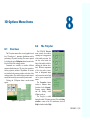
lîÉêîáÉï =K=K=K=K=K=K=K=K=K=K=K=K=K=K=K=K=K=K=K=K=K=K=K=K=K=K=K=K=K=K=KVP
qÜÉ=qêáÅóÅäÉê K=K=K=K=K=K=K=K=K=K=K=K=K=K=K=K=K=K=K=K=K=K=K=K=K=K=K=K=KVP
sáëì~äáòÉ =K=K=K=K=K=K=K=K=K=K=K=K=K=K=K=K=K=K=K=K=K=K=K=K=K=K=K=K=K=K=K=KVQ
UKQ=
UKR=
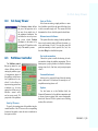
`ìíJ^ï~ó=sáÉïÉê K=K=K=K=K=K=K=K=K=K=K=K=K=K=K=K=K=K=K=K=K=K=K=K=K= VR
m~íÜäáåÉë=`çåíêçääÉê K=K=K=K=K=K=K=K=K=K=K=K=K=K=K=K=K=K=K=K=K=K=K= VR
VK=cbcilt=íççäë =K=K=K=K=K=K=K=K=K=K=K=K=K=K=K=K=K=K=K=K=K=K=K=K=K=K=K=K=K=K=K=K=K=K=K=K=K=K=K=K=K=K=K=K=K=K=K=K=K=K VT
VKN=
VKNKN=
VKNKO=
VKNKP=
VKO=
VKOKN=
VKOKO=
VKOKP=
VKOKQ=
cbmilq K=K=K=K=K=K=K=K=K=K=K=K=K=K=K=K=K=K=K=K=K=K=K=K=K=K=K=K=K=K=K=K=KVT
dÉåÉê~ä=ëÉííáåÖë =K=K=K=K=K=K=K=K=K=K=K=K=K=K=K=K=K=K=K=K=K=K=K=K=K=KVT
lÄàÉÅíë K=K=K=K=K=K=K=K=K=K=K=K=K=K=K=K=K=K=K=K=K=K=K=K=K=K=K=K=K=K=K=K=KVT
`êÉ~íáåÖ=~=éäçí=Åçãéçëáíáçå=K=K=K=K=K=K=K=K=K=K=K=K=K=K=K=K=KVU
cbJij² =K=K=K=K=K=K=K=K=K=K=K=K=K=K=K=K=K=K=K=K=K=K=K=K=K=K=K=K=K=K=K=KNMN
tÜ~í=áë=cbJijO=~åÇ=ïÜÉå=áë=áí=ìëÉÑìä\K=K=K=K=K=K=K=K=KNMN
m~ê~ãÉíÉê=Éëíáã~íáçå=Äó=
êÉëáÇì~ä=ãáåáãáò~íáçå =K=K=K=K=K=K=K=K=K=K=K=K=K=K=K=K=K=K=K=K=KNMN
a~í~=áåéìí=ÑáäÉ K=K=K=K=K=K=K=K=K=K=K=K=K=K=K=K=K=K=K=K=K=K=K=K=K=K=KNMN
iç~ÇáåÖ=íÜÉ=Ç~í~=ëÉí K=K=K=K=K=K=K=K=K=K=K=K=K=K=K=K=K=K=K=K=K=KNMP
VKOKR=
VKOKS=
VKOKT=
VKOKU=
VKOKV=
VKOKNM=
VKOKNN=
VKOKNO=
`çåíêçä=Çá~äçÖ K=K=K=K=K=K=K=K=K=K=K=K=K=K=K=K=K=K=K=K=K=K=K=K=K=K= NMQ
a~í~Jéäçí=îáÉï K=K=K=K=K=K=K=K=K=K=K=K=K=K=K=K=K=K=K=K=K=K=K=K=K=K= NMR
a~í~JîáÉï=Åìêëçê=ãçÇÉë =K=K=K=K=K=K=K=K=K=K=K=K=K=K=K=K=K=K= NMT
pÉäÉÅíáåÖ=~åÇ=ìåëÉäÉÅíáåÖ=Ç~í~=éçáåíë=Ñçê=ïÉáÖÜí=
ãçÇáÑáÅ~íáçå =K=K=K=K=K=K=K=K=K=K=K=K=K=K=K=K=K=K=K=K=K=K=K=K=K=K=K= NMT
tÉáÖÜí=ãçÇáÑáÅ~íáçå =K=K=K=K=K=K=K=K=K=K=K=K=K=K=K=K=K=K=K=K=K= NMT
a~í~JîáÉï=å~îáÖ~íáçå K=K=K=K=K=K=K=K=K=K=K=K=K=K=K=K=K=K=K=K=K= NMU
a~í~JîáÉï=ÅäçåáåÖ=K=K=K=K=K=K=K=K=K=K=K=K=K=K=K=K=K=K=K=K=K=K=K= NMV
bñéçêíáåÖ=Ç~í~=Ñáíë K=K=K=K=K=K=K=K=K=K=K=K=K=K=K=K=K=K=K=K=K=K=K= NMV
m~êí=ff==qìíçêá~ä
NMK=qìíçêá~ä =K=K=K=K=K=K=K=K=K=K=K=K=K=K=K=K=K=K=K=K=K=K=K=K=K=K=K=K=K=K=K=K=K=K=K=K=K=K=K=K=K=K=K=K=K=K=K=K=K=K=K=K=K NNP
NMKN=
fåíêçÇìÅíáçå=K=K=K=K=K=K=K=K=K=K=K=K=K=K=K=K=K=K=K=K=K=K=K=K=K=K=K=KNNP
NMKNKN= ^Äëíê~Åí =K=K=K=K=K=K=K=K=K=K=K=K=K=K=K=K=K=K=K=K=K=K=K=K=K=K=K=K=K=K=KNNP
NMKNKO= pÅçéÉ=~åÇ=ëíêìÅíìêÉ=çÑ=íÜÉ=íìíçêá~ä =K=K=K=K=K=K=K=K=K=K=KNNP
NMKO=
pÅÉå~êáç=K=K=K=K=K=K=K=K=K=K=K=K=K=K=K=K=K=K=K=K=K=K=K=K=K=K=K=K=K=K=KNNQ
NMKOKN= qÜÉ=q~ëâ K=K=K=K=K=K=K=K=K=K=K=K=K=K=K=K=K=K=K=K=K=K=K=K=K=K=K=K=K=K=KNNQ
NMKP=
qÜÉ=Oa=jçÇÉäK=K=K=K=K=K=K=K=K=K=K=K=K=K=K=K=K=K=K=K=K=K=K=K=K=K=KNNS
NMKPKN= píÉé=N=J=_~ëáÅ=ëíêìÅíìêÉ=K=K=K=K=K=K=K=K=K=K=K=K=K=K=K=K=K=K=K=KNNS
NMKPKNKN= aÉëáÖåáåÖ=íÜÉ=ëìéÉêÉäÉãÉåí=ãÉëÜ =K=K=K=K=K=K=K=K=K=K=KNNS
NMKPKNKO= dÉåÉê~íáåÖ=íÜÉ=ÑáåáíÉ=ÉäÉãÉåí=ãÉëÜ =K=K=K=K=K=K=K=K=K=KNNT
NMKPKO= píÉé=O=J=bÇáíáåÖ=íÜÉ=éêçÄäÉã=é~ê~ãÉíÉêëK=K=K=K=K=K=KNNV
NMKPKOKN= mêçÄäÉã=Åä~ëë =K=K=K=K=K=K=K=K=K=K=K=K=K=K=K=K=K=K=K=K=K=K=K=K=K=K=KNNV
NMKPKOKO= cäçï=Ç~í~ =K=K=K=K=K=K=K=K=K=K=K=K=K=K=K=K=K=K=K=K=K=K=K=K=K=K=K=K=K=KNNV
NMKPKOKP= oÉÑÉêÉåÅÉ=Ç~í~ =K=K=K=K=K=K=K=K=K=K=K=K=K=K=K=K=K=K=K=K=K=K=K=K=K=KNOO
NMKPKP= píÉé=P=J=iÉíÛë=íÉëí=áí =K=K=K=K=K=K=K=K=K=K=K=K=K=K=K=K=K=K=K=K=K=K= NOP
NMKPKPKN= oìååáåÖ=íÜÉ=ëáãìä~íçê K=K=K=K=K=K=K=K=K=K=K=K=K=K=K=K=K=K=K=K= NOP
NMKPKPKO= e~äí=~åÇ=îáÉï=êÉëìäíë=K=K=K=K=K=K=K=K=K=K=K=K=K=K=K=K=K=K=K=K=K= NOP
NMKPKQ= píÉé=Q=J=_~Åâ=íç=íÜÉ=éêçÄäÉã=ÉÇáíçê=~åÇ=êìå=~Ö~áåK=K=
=K=K=K=K=K=K=K=K=K=K=K=K=K=K=K=K=K=K=K=K=K=K=K=K=K=K=K=K=K=K=K=K=K=K=K=K=K= NOP
NMKPKQKN= mêçÄäÉã=Åä~ëëK=K=K=K=K=K=K=K=K=K=K=K=K=K=K=K=K=K=K=K=K=K=K=K=K=K=K= NOP
NMKPKQKO= qÉãéçê~ä=C=Åçåíêçä=Ç~í~ K=K=K=K=K=K=K=K=K=K=K=K=K=K=K=K=K=K= NOQ
NMKPKQKP= cäçï=Ç~í~K=K=K=K=K=K=K=K=K=K=K=K=K=K=K=K=K=K=K=K=K=K=K=K=K=K=K=K=K=K= NOQ
NMKPKQKQ= qê~åëéçêí=Ç~í~ K=K=K=K=K=K=K=K=K=K=K=K=K=K=K=K=K=K=K=K=K=K=K=K=K=K= NOU
NMKPKQKR= páãìä~íçêK=K=K=K=K=K=K=K=K=K=K=K=K=K=K=K=K=K=K=K=K=K=K=K=K=K=K=K=K=K= NPN
NMKPKR= píÉé=R=J=^å~äóòáåÖ=íÜÉ=êÉëìäíëK=K=K=K=K=K=K=K=K=K=K=K=K=K=K= NPN
NMKPKRKN= qÜÉ=éçëíéêçÅÉëëçê=K=K=K=K=K=K=K=K=K=K=K=K=K=K=K=K=K=K=K=K=K=K=K= NPN
NMKPKS= `çåÅäìëáçåë=Ñçê=íÜÉ=Oa=ãçÇÉä K=K=K=K=K=K=K=K=K=K=K=K=K=K= NPT
cbcilt=RKN=ö=î
`çåíÉåíë
NMKQ=
qÜÉ=Pa=jçÇÉäK=K=K=K=K=K=K=K=K=K=K=K=K=K=K=K=K=K=K=K=K=K=K=K=K=K=KNPU
NMKQKN= eçï=íç=ÖÉí=íÜÉ=Ç~í~=K=K=K=K=K=K=K=K=K=K=K=K=K=K=K=K=K=K=K=K=K=KNPU
NMKQKO= píÉé=N=J=aÉëáÖåáåÖ=ëäáÅÉë=~åÇ=ä~óÉêë K=K=K=K=K=K=K=K=K=K=KNPU
NMKQKOKN= Pa=päáÅÉ=ÉäÉî~íáçå=K=K=K=K=K=K=K=K=K=K=K=K=K=K=K=K=K=K=K=K=K=K=K=KNQN
NMKQKOKO= oÉÅçåÑáÖìêÉ=Pa=í~ëâ =K=K=K=K=K=K=K=K=K=K=K=K=K=K=K=K=K=K=K=K=K=KNQN
NMKQKP= píÉé=O=J=^ëëáÖåãÉåí=~åÇ=Åçåíêçä=áå=íÜÉ=éêçÄäÉã=ÉÇáíçê
K=K=K=K=K=K=K=K=K=K=K=K=K=K=K=K=K=K=K=K=K=K=K=K=K=K=K=K=K=K=K=K=K=K=K=K=K=KNQO
NMKQKPKN= mêçÄäÉã=Åä~ëë =K=K=K=K=K=K=K=K=K=K=K=K=K=K=K=K=K=K=K=K=K=K=K=K=K=K=KNQO
NMKQKPKO= cäçï=áåáíá~äë K=K=K=K=K=K=K=K=K=K=K=K=K=K=K=K=K=K=K=K=K=K=K=K=K=K=K=K=KNQP
NMKQKPKP= cäçï=ÄçìåÇ~êáÉë =K=K=K=K=K=K=K=K=K=K=K=K=K=K=K=K=K=K=K=K=K=K=K=K= NQP
NMKQKPKQ= ^ëëáÖåáåÖ=~åÇ=ÅÜÉÅâáåÖ=íÜÉ=íê~åëéçêí=Ç~í~ =K=K=K=K= NQQ
NMKQKQ= píÉé=P=J=mçëíéêçÅÉëëáåÖ=áå=Pa =K=K=K=K=K=K=K=K=K=K=K=K=K=K= NQR
NMKQKQKN= oÉëìäíë=îáÉïÉê =K=K=K=K=K=K=K=K=K=K=K=K=K=K=K=K=K=K=K=K=K=K=K=K=K=K= NQR
NMKQKQKO= _ìÇÖÉí=ãÉåìK=K=K=K=K=K=K=K=K=K=K=K=K=K=K=K=K=K=K=K=K=K=K=K=K=K=K= NQR
NMKQKQKP= cäìáÇJÑäìñ=~å~äóòÉê=K=K=K=K=K=K=K=K=K=K=K=K=K=K=K=K=K=K=K=K=K=K=K= NQS
NMKQKR= píÉé=Q=J=Pa=léíáçåë=ãÉåìK=K=K=K=K=K=K=K=K=K=K=K=K=K=K=K=K= NQT
NMKQKS= cáå~ä=êÉã~êâë K=K=K=K=K=K=K=K=K=K=K=K=K=K=K=K=K=K=K=K=K=K=K=K=K=K=K= NQU
NMKR=
iáëí=çÑ=ÑáäÉë=K=K=K=K=K=K=K=K=K=K=K=K=K=K=K=K=K=K=K=K=K=K=K=K=K=K=K=K=K= NQV
m~êí=fff==fåíÉêÑ~ÅÉ=j~å~ÖÉê
NNK=mêçÖê~ããáåÖ=fåíÉêÑ~ÅÉ K=K=K=K=K=K=K=K=K=K=K=K=K=K=K=K=K=K=K=K=K=K=K=K=K=K=K=K=K=K=K=K=K=K=K=K=K=K=K=K= NRP
NNKN=
NNKNKN=
NNKNKO=
NNKO=
NNKOKN=
NNKOKO=
fåíêçÇìÅíáçå=K=K=K=K=K=K=K=K=K=K=K=K=K=K=K=K=K=K=K=K=K=K=K=K=K=K=K=KNRP
`çããçå=íÉêãëK=K=K=K=K=K=K=K=K=K=K=K=K=K=K=K=K=K=K=K=K=K=K=K=K=KNRS
^ÄÄêÉîá~íáçåë =K=K=K=K=K=K=K=K=K=K=K=K=K=K=K=K=K=K=K=K=K=K=K=K=K=K=KNRS
fåíÉêÑ~ÅÉ=j~å~ÖÉê=Ñçê=rëÉêë =K=K=K=K=K=K=K=K=K=K=K=K=K=K=K=KNRT
jçÇìäÉ=ÅçåÑáÖìê~íáçå K=K=K=K=K=K=K=K=K=K=K=K=K=K=K=K=K=K=K=K=KNRT
oÉÖáëíÉêáåÖ=~=ãçÇìäÉ =K=K=K=K=K=K=K=K=K=K=K=K=K=K=K=K=K=K=K=K=KNRT
NNKOKP= jçÇìäÉ=éêçéÉêíáÉë K=K=K=K=K=K=K=K=K=K=K=K=K=K=K=K=K=K=K=K=K=K=K= NRU
NNKOKQ= eçï=íç=ìëÉ=ÉñíÉêå~ä=ãçÇìäÉëK=K=K=K=K=K=K=K=K=K=K=K=K=K=K= NRU
NNKOKQKN= =fåíÉêÑ~ÅÉ=ëáãìä~íáçåW=~íí~ÅÜáåÖ=~=ãçÇìäÉ=íç=~=cbj=
éêçÄäÉãK=K=K=K=K=K=K=K=K=K=K=K=K=K=K=K=K=K=K=K=K=K=K=K=K=K=K=K=K=K=K= NRU
NNKOKQKO= =fåíÉêÑ~ÅÉ=êÉÖáçå~äáò~íáçåW=Ç~í~Ä~ëÉ=êÉÖáçå~äáò~íáçå=ÇáJ
~äçÖ K=K=K=K=K=K=K=K=K=K=K=K=K=K=K=K=K=K=K=K=K=K=K=K=K=K=K=K=K=K=K=K=K=K= NRV
pìÄàÉÅí=fåÇÉñ K=K=K=K=K=K=K=K=K=K=K=K=K=K=K=K=K=K=K=K=K=K=K=K=K=K=K=K=K=K=K=K=K=K=K=K=K=K=K=K=K=K=K=K=K=K=K=K=K=K=K= NSN
îá=ö=rëÉêÛë=j~åì~ä
tÜ~íÛë=åÉï=áå=cbcilt=RKN
tÜ~íÛë=åÉï=áå=cbcilt=RKN
This preface addresses the experienced user who is
interested in an overview of the new capabilities of
FEFLOW 5.1 compared to the previous release 5.0.
Improvements are listed and references to the detailed
description of the features in the different FEFLOW
manuals are provided. The novice user might skip this
section and start with Part I of the manual.
A newsgroup has been set up in addition to the
online help and different manuals. Look for details at
www.wasy.de/english/service/newsgroups.html.
The new functions in FEFLOW 5.1 can be divided
in following three main parts:
√ãçÇÉä=êÉäÉî~åí=ÅÜ~åÖÉë
√ìëÉê=áåíÉêÑ~ÅÉ=ÅÜ~åÖÉë
√éêçÖê~ã=áåíÉêÑ~ÅÉ=ÅÜ~åÖÉë
jçÇÉä=êÉäÉî~åí=ÅÜ~åÖÉë
Oa=î~êá~ÄäÉJÇÉåëáíó=Ñäçï=~åÇ=íê~åëéçêí=ãçÇJ
ÉäáåÖ=ïáíÜ=éêçàÉÅíÉÇ=Öê~îáíó=ÑáÉäÇ
It allows the 2D density-dependent modeling for
confined aquifers by projecting a 3D gravity field onto
a horizontal planar model area. A typical application is
the transport of brines in thin aquifer layers of sloped
geometry (basin). Instead of running a full 3D variabledensity flow and transport model, the gravity-projected
2D model option significantly simplifies the computations.
fåíÉêÑ~ÅÉ=íç=qof^kdib=ãÉëÜ=ÖÉåÉê~íçê
An interface to the mesh generator TRIANGLE,
copyright© by J. R. Shewchuk (University of California at Berkeley) for complex superelement meshes is
integrated. The generator is very fast and especially
convenient for superelement meshes which include a
large number of add-ins.
^äÖÉÄê~áÅ=ãìäíáÖêáÇ=ëçäîÉê=p^jd
SAMG, copyright© by K. Stüben (FhG-SCAI),
allows the efficient solution of large and complex
cbcilt=RKN=ö=T
tÜ~íÛë=åÉï=áå=cbcilt=RKN
sparse-matrix systems by the algebraic multigrid
method. Special cases involving large parameter contrasts or large number of unknowns can be solved faster
by SAMG than by the preconditioned conjugate-gradient iterative solver (PCG). The algebraic multigrid
method solves a defined matrix system on a reasonable
hierarchy of grids, which is automatically constructed
based on the algebraic information explicitly and
implicitly contained in the discretization.
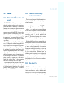
bèì~íáçå=ëçäîÉê=ëÉííáåÖë=
The equation solver settings can be modified by
special dialogs (e.g., iteration stop criterion, maximum
iteration numbers).
dÉçÖê~éÜáÅ~ä=íê~åëÑçêã~íáçå=
An extended set of geographical transformation
methods are provided for superelement meshes and
finite-element models. An affine transformation is
included in the FEFLOW license as a default method,
additional methods, especially for Germany, can be
licensed separately.
U=ö=rëÉêÛë=j~åì~ä
s~êá~ÄäÉJÇÉåëáíó=ã~ëë=íê~åëéçêí=
The maximum concentration Cs can be modified in
the reference mass dialog. Thus the density ratio can be
used correctly even if the initial maximum concentration is 0 mg/l.
rëÉê=áåíÉêÑ~ÅÉ=ÅÜ~åÖÉë
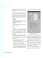
cáäÉJëÉäÉÅíáçå=Çá~äçÖ
The default Windows file-selection dialog has been
implemented in the new version. It replaces the previous Motif-style selection box. Helpful functions such
as Managing of file directories or Add favorite directories are available.
lÄëÉêî~íáçå=éçáåíë
Observation points now have properties for labeling
and providing drawing attributes. Automatic import
and name assignment from shp-files is possible. All
attributes can be edited and arbitrary points can be
deleted interactively. The following import formats
have been added: PNT, DXF, SHP, TRP.
qê~åëáÉåí=ÄçìåÇ~êáÉë=~åÇ=ã~íÉêá~äë
When reducing a transient model to a steady state
model, all time-dependent data (boundary conditions,
constraint conditions, material properties) are easily
reduced to steady-state conditions.
pìéÉêÉäÉãÉåí=ãÉëÜ
Edge attributes (linear or parabolic) are saved in the
superelement smh-file.
m~íÜäáåÉ=Åçãéìí~íáçå=
The existing data sets (transport data and constant
value) to derive porosity values for the computation of
isochrones were extended. The storativity data set can
be used alternatively now.
m~íÜäáåÉ=Éñéçêí
Pathline export in 2D and 3D with corresponding
attributes (velocities, isochrones) is available in new
formats (DXF, SHP, DAT, PNT, PLX, DBF). Additionally, there is a new Export button for exporting 3D
pathline vertices.
bñéçêíáåÖ=ÉäÉãÉåí~ä=~åÇ=åçÇ~ä=èì~åíáíáÉë
Exporting elemental and nodal quantities and
boundary conditions with attributes is possible for a
current slice/layer or for all slices/layers.
cê~ÅíìêÉ=ÉäÉãÉåíë
The new version 5.1 allows copying of fracture elements for slices in 3D.
içÖ=jÉëë~ÖÉë=Äçñ
The FEFLOW Log messages box can be easily
saved to an arbitrary destination by using the new file
selection dialog.
_~íÅÜ=ãçÇÉ
The complete graphical output can be suppressed
using batch mode, resulting in faster simulations.
aá~Öê~ã=ÅìêîÉë
All curves from diagrams in the simulator (e.g.,
hydraulic head, flux) are saved in the dac file including all time steps. Consequently, important information
from the observation points/groups can be fully reconstructed in the postprocessor.
mêçÖê~ããáåÖ=áåíÉêÑ~ÅÉ
cáäíÉê=
New filters are available to import superelement
meshes or finite element meshes based on shp-files,
dxf-files and ASCII-files.
fcj
bñéçêí=çÑ=ÑêáåÖÉÇ=áëçäáåÉë
The export of fringed isolines is available for quadrilateral elements, too.
IFM modules can now integrate Windows dialogs,
e.g., using Microsoft Foundation Classes for programming. There are many new API functions for unsaturated flow, for adaptive meshes, for budgeting, and
more. The online help gives more information including an exact description of these new functions.
^ìíçã~íáÅ=êÉÖáçå~äáò~íáçå
Automatic assignment of boundary conditions and
corresponding constraint conditions (also time dependent) has been implemented. Additionally, the Join tool
can be used for initial conditions and elevations.
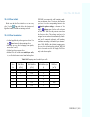
The following table lists the new features which are
described in more detail in the FEFLOW documentation and in the online help.
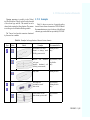
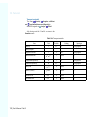
Table: New features in FEFLOW 5.1
Feature
Reference
2D variable-density flow and transport modeling with projected gravity
field
White papers Vol. III, Chapter 1
Interface to TRIANGLE mesh generator
User’s manual, page 39
cbcilt=RKN=ö=V
tÜ~íÛë=åÉï=áå=cbcilt=RKN
Table: New features in FEFLOW 5.1 (continued)
Feature
NM=ö=rëÉêÛë=j~åì~ä
Reference
Algebraic multigrid solver SAMG
White papers Vol. III, Chapter 3;
User’s manual, page 23
Equation solver settings
User’s manual, page 24
Geographical transformation
User’s manual, page 32
Transient boundaries to steady state conditions
User’s manual, page 47
Pathline computation
FEFLOW Online Help
Variable density mass transport
FEFLOW Online Help
File selection box
User’s manual, page 20
Observation points
User’s manual, page 66
Superelement mesh
User’s manual, page 32
Pathline export
User’s manual, page 17
Fracture elements
User’s manual, page 68
Log messages box
User’s manual, page 73
Batch mode
FEFLOW Online Help
Diagram curves
FEFLOW Online Help
Filter
FEFLOW Online Help
IFM
FEFLOW Online Help
m~êí=f
jÉåì=dìáÇÉ
cbcilt=RKN=ö=NN
NO=ö=rëÉêÛë=j~åì~ä=J=m~êí=f
N
qÜÉ=cbcilt=pÜÉää
N
qÜÉ=cbcilt=pÜÉää=
NKN
fåíêçÇìÅíáçå
The graphical FEFLOW Shell contains a large
amount of commands on several menu levels. Pop-up
menus provide additional information. The purpose of
Part I is to give a detailed overview of the commands.
It can be used as a reference, or it can be perused by
users new to FFLOW.
We recommend that you try running FEFLOW
before reading past this manual: Please try to perform a
first FEFLOW simulation run using the Demonstration
Exercise. More information is available from the online
Help files. Online Help is invoked by pressing the
Help button in some of the menus or by hitting <F1>.
If a problem cannot be solved by the information found
in this manual, you can look in the online Help files for
additional information. Online Help will allow you to
quickly and effectively continue your use of FEFLOW.
Some conventions are necessary to clearly describe
the Shell. This manual contains a section for each command or closely related group of commands. Important
pull-down, pop-up, and cascade menus are illustrated.
The commands are presented as they would be encountered if you start at the left of the top level menu (Shell)
and go down each pull-down menu. The explanation
continues with the next branch to the right in the Shell
menu. While running FEFLOW, you can quickly find
the reference information of a command by noting the
location of the command in the menu structure and
finding the corresponding section in this manual. Alternative commands are suggested when appropriate.
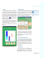
NKO
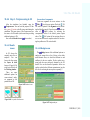
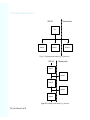
m~êíë=çÑ=íÜÉ=pÜÉää
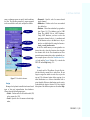
The Shell provides a variety of command sequences
to formulate and simulate a given problem. It consists
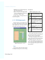
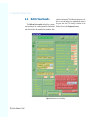
of four main parts, which are illustrated in Section Figure 1.1. The working window displays the model with
its mesh, boundary conditions, etc., depending on the
current operation context. All mouse-based editing is
performed here. The shell menu gives access to the different parts and functions of FEFLOW. The menu
structure is listed in Figure 1.3. The control panel
offers information about the model view and provides
tools for zooming and 3D visualization.
cbcilt=RKN=ö=NP
NK=qÜÉ=cbcilt=pÜÉää
pÜÉää=ãÉåì
tçêâáåÖ=ïáåÇçï
fåÑç
ÄçñÉë
jÉëë~ÖÉ=Ä~ê
Figure 1.1 Parts of the Shell.
kçíáÅÉW= qÜÉ= nìáÅâ
^ÅÅÉëë= ãÉåì= ÅçåJ
í~áåë= ëçãÉ= çÑ= íÜÉ
çéíáçåë= çÑ= íÜÉ= cáäÉ= ãÉåìK
vçì=Å~å=ìëÉ=íÜÉëÉ=çéíáçåë=íç
ë~îÉ= Ç~í~= ~åÇ= ã~å~ÖÉ
Ä~ÅâÖêçìåÇ= ã~éëK= fí= áë
~î~áä~ÄäÉ= çå= ÉîÉêó= äÉîÉä= çÑ
cbcilt= Äó= ÅäáÅâáåÖ= íÜÉ
Åçãéìí~íáçå~ä=ëí~íìë=Ä~êK
kçíáÅÉW= vçì= Å~å
ë~îÉ= ÉÇáíÉÇ= éêçÄJ
äÉã= Ç~í~= áããÉÇáJ
~íÉäó= Äó= ÅäáÅâáåÖ= íÜÉ
Åçãéìí~íáçå~ä=ëí~íìë=Ä~ê=áå
íÜÉ= nìáÅâ= ^ÅÅÉëë= éçéJìé
ãÉåìK=
NQ=ö=rëÉêÛë=j~åì~ä=J=m~êí=f
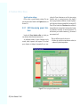
Clicking in the green field which shows the current
element type and the progress bar activates the quickaccess menu (Figure 1.2) which provides direct access
to some of the functions available in the File menu. In
the message bar at the bottom of the screen you can
find context-sensitive help concerning the operations
which you are about to perform, e.g., active hot keys.
NKP
qÜÉ=jÉåì=eáÉê~êÅÜó
The FEFLOW Shell menu is the top level of a
detailed menu structure. The structure is based in part
on practical criteria so that basic and often-used settings can be accessed directly from the Shell menu. The
lower-level menus follow the sequence of steps of
model creation. The basic steps are listed in Table 1.1
together with the corresponding menu names and the
sections of this manual that describe them.
Table 1.1 The basic steps of modeling
Topic
Names
Section
Number
mesh design
Mesh Editor
mesh generation
Mesh Generator
Section 4
attribute
tion
Problem Editor
Section 5
simulation
Simulator Run
Section 6
postprocessing
Postprocessor
Section 7
specifica-
Section 3
Figure 1.3 The Shell menu with its ten submenus.
Figure 1.2 Quick access menu.
NKQ=qÜÉ=wççãáåÖ=cìåÅíáçå
Figure 1.3 FEFLOW Shell menu structure.
NKQ
qÜÉ=wççãáåÖ=cìåÅíáçå
The zooming function lets you zoom in and out by
dragging a rectangle with the mouse. There is no limiting zoom factor. Activating the
button and clicking at any point of interest zooms in with a
magnification factor of two. Draw a rectangle with the
left or middle mouse button pressed to zoom in or out,
respectively.
After activating the
button it is possible to
move the visible extent of the model with the mouse.
The scale of the view is preserved.
The
button returns to the previous view extent.
For this purpose the last ten view extents are stored.
The
button resets the view to the default extent
NKR
aáëéä~ó= çÑ= íÜÉ= tçêâáåÖ
táåÇçï
Additionally to the zooming functions the working
window can be adjusted by specifying width and exaggeration of the view. Besides editing the values directly
some functions are provided in pop-up menus, which
can be invoked by clicking on one of the arrows.
kçíáÅÉW=`Ü~åÖÉë=áå
éêçÄäÉã= ïáÇíÜ= çê
Éñ~ÖÖÉê~íáçå= ã~ÇÉ
ìëáåÖ= íÜÉ= Çáëéä~ó= çéíáçåë
~ÑÑÉÅí= çåäó= íÜÉ= ãçÇÉä= îáÉïK
rëÉ= íÜÉ= mêçÄäÉã= jÉ~ëìêÉ
ãÉåì= íç= ÅÜ~åÖÉ= ÅççêÇáJ
å~íÉë=çê=éÜóëáÅ~ä=ÉñíÉåíK
cbcilt=RKN=ö=NR
NK=qÜÉ=cbcilt=pÜÉää
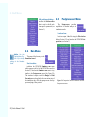
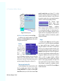
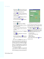
NKS
qÜÉ=j~é=j~å~ÖÉê
please refer to the FEFLOW online help.
The map manager is a comfortable tool to handle
different types of background maps (ASCII point, line
and polygon files, ESRI shape files, CAD data and
image files). It is opened via the Quick Access Menu or
the File menu.
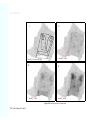
Figure 1.5 Map ID editor.
Figure 1.4 Map manager.
For the procedure of adding maps please have a
look at the Demonstration Exercise.
In the map manager all currently loaded maps are
listed. The uppermost map in the list is shown in the
background, whereas the lowest one forms the foreground. At the left side of each map title a small button
allows to switch maps on and off for the view. Selecting a map and clicking the Colors button opens the
Map ID editor, which offers functionality to set numerous display options for the map. Please note that the
following description is only valid for the true-color
display mode. For color settings in pseudo-color mode
NS=ö=rëÉêÛë=j~åì~ä=J=m~êí=f
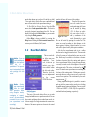
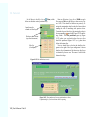
The left part of the Map ID Editor shows a list of all
IDs of the current map. The IDs can be switched on and
off for the view using the respective button on the left.
If one or several of the IDs have been selected, their
properties can be changed in the right part of the window. The seven switches should be self-explanatory, a
detailed description can be found in the online help.
Note that transparent polygon filling is obtained using
the last entry in the Fill style section:
If several IDs have been selected containing different settings for an option, a multi-selection icon is
shown:
Click the ’Apply’ button to apply the changes.
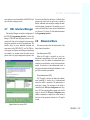
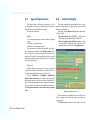
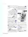
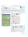
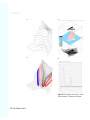
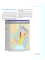
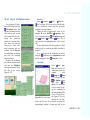
NKT=qÜÉ=Pa=léíáçåë=jÉåì
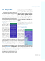
NKT
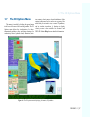
qÜÉ=Pa=léíáçåë=jÉåì
This menu is invoked by clicking the green button
in the lower left corner of the working window. The 3D
Options menu allows the visualization of a threedimensional problem as line and fringe drawings for
conductivity values, hydraulic head, saturation, mois-
ture content, velocity, mass, or heat distributions. Other
options in this menu can be used to cut out parts of the
model body for an inside view, to create 3D pathlines,
and to visualize isosurfaces. A function to display
velocity vectors is also available. See Section 8 and
FEFLOW Online Help for more detailed information.
Figure 1.6 The 3D option menu in displaying, for instance, 3D pathlines.
cbcilt=RKN=ö=NT
NK=qÜÉ=cbcilt=pÜÉää
NU=ö=rëÉêÛë=j~åì~ä=J=m~êí=f
O
pÜÉää=jÉåì
O
access to other parts of the Shell hierarchy.
pÜÉää=jÉåì=
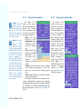
OKN
fåíêçÇìÅíáçå
The FEFLOW graphical Shell contains several levels of menu commands. Section 2 describes the top
level of the Shell. Subsequent sections will cover the
lower level commands. Figure 2.1 shows the Shell
menu.
Figure 2.1 Shell menu.
The following subsections briefly describe the ten
submenus: File, Edit, Run, Postprocessor, Options,
IFM, Dimension, Tools, Windows and Info. The Quick
Access menu (Figure 2.2) is a pop-up menu containing
some Shell main-menu items. It is activated by clicking
on the green field on the left side of the screen.
All menu and submenu items are selected by clicking the mouse on the item, or by typing the key corresponding to the underlined letter in the item. Inactive
menu items are shown in grey. Selecting the menu item
in the lowest position of a pull-down menu will often
return you to the master Shell menu. This allows quick
Figure 2.2 Quick access menu.
cbcilt=RKN=ö=NV
OK=pÜÉää=jÉåì
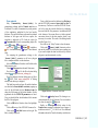
OKO
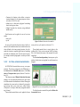
cáäÉ=jÉåì
The File menu
allows you to load
and save all the files
necessary for a
FEFLOW session.
The following paragraphs explain the
options in this menu
iç~Ç=ëìéÉêÉäÉJ
ãÉåí=ãÉëÜ=KKK
This option loads an
existing
superelement mesh via the
FEFLOW file-selection dialog. It also
starts the Mesh editor.
Figure
2.3
shows the File selection dialog that queries you for a
filename.
p~îÉ=ëìéÉêÉäÉãÉåí=ãÉëÜ=KKK
Saves the superelement-mesh data you have created.
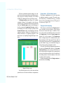
iç~Ç=ÑáåáíÉ=ÉäÉãÉåí=éêçÄäÉã=KKK
Loads an existing finite-element problem by invoking the FEFLOW file-selection dialog (Figure 2.3).
p~îÉ=ÑáåáíÉ=ÉäÉãÉåí=éêçÄäÉã=KKK
Saves the complete data for the current finite-element problem. Note that this does not include the
superelement mesh.
OM=ö=rëÉêÛë=j~åì~ä=J=m~êí=f
Figure 2.3 FEFLOW file-selection dialog (Windows XP).
The file-selection dialog offers to Add favorite
directories
and to Manage favorite directories
(Windows operating systems only).
^ÇÇ=ã~é=KKK
The Add map option opens a File selection dialog
for importing different types of background maps. The
list includes: FEFLOW files, Raster Images, HPGL
files, ARC/INFO Generate format-files, ArcView compatible shape files, DXF or triplet files.
j~é=ã~å~ÖÉê=KKK
This selection opens a submenu for activating or
erasing background maps. For detailed information see
FEFLOW online Help.
OKP=bÇáí=jÉåì
fãéçêí=ÑáäíÉê=L=bñéçêí=ÑáäíÉê
These options manage the loading and saving of
data files in additional formats. They are only shown
when a folder named ’filter’ exists within the
FEFLOW home directory. The import of complete data
files from the finite-element package Sick 100 is currently supported. The import of superelement meshes is
possible in the ASCII Generate Polygon format. All
import filters are available on both UNIX and Windows. You can easily add filters for your own data formats. See online Help for more detailed information.
mêáåí=KKK=EtáåÇçïë=çåäóF
Starts the FEPLOT print tool for automatic visualization of the plot files captured during the current session. The plot files can be saved in FEFLOW on
UNIX, too. These files can be subsequently visualized
in FEPLOT on a Windows based PC (see also Section
9.1).
oÉÅÉåí=cbjLa^`Lpje=ÑáäÉë
Any of the six most recently used files of each type
can be loaded directly from here.
OKP
bÇáí=jÉåì
This menu is invoked to set
up a FEFLOW problem. The
following paragraphs explain
the commands in this menu:
aÉëáÖå=ëìéÉêÉäÉãÉåí=
jÉëÜKKK
invokes the Mesh editor for
designing a superelement
mesh. It uses the mouse (as
the basic input environment)
or the keyboard. Geometric
data for a study area is entered
using the FEFLOW Mesh
editor (see Section 3).
kçíáÅÉW= qÜÉ=ë~îáåÖ
çéíáçåë= ^ÇÇ= ã~éI
j~é=ã~å~ÖÉêI=~åÇ
mêáåí=~êÉ=~äï~óë=~î~áä~ÄäÉ=áå
íÜÉ= nìáÅâ= ^ÅÅÉëë= ãÉåìI
áåîçâÉÇ= Äó= ÅäáÅâáåÖ= çå= íÜÉ
ÖêÉÉå=ÑáÉäÇ=íç=íÜÉ=äÉÑí=çÑ=íÜÉ
ïçêâáåÖ= ïáåÇçï= EcáÖìêÉ
OKOFK=
dÉåÉê~íÉ=ÑáåáíÉ=ÉäÉãÉåí=
ãÉëÜKKK
opens the Mesh generator
for creating a finite-element
mesh within the designed
superelement mesh (see Section 4).
cbcilt=RKN=ö=ON
OK=pÜÉää=jÉåì
bÇáí=éêçÄäÉã=~ííêáÄìíÉëKKK
invokes the Problem editor
that is used to edit all problem-specific parameters (see
Section 5).
OKR
mçëíéêçÅÉëëçê=jÉåì
The Postprocessor provides
capabilities for detailed analysis of
simulation results.
iç~Ç=~åÇ=êìåKKK
loads an output *.dac file using the File-selection
dialog (Section 2.2) and invokes the FEFLOW Postprocessor (see Section 7).
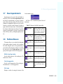
OKQ
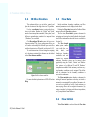
oìå=jÉåì
kçíáÅÉW= rëÉ= íÜÉ
This menu offers the entry to the
léíáçåë=jÉåì=EpÉÅJ
íáçå= OKSF= íç= ãçÇáÑó Simulation kernel:
ëÉííáåÖë= Ñçê= íÜÉ= páãìä~íçê
pí~êí=ëáãìä~íçêKKK
hÉêåÉäK
initializes the FEFLOW Simulator run menu
which appears to the left of the FEFLOW screen (See
Section 6). Note that the Simulator run menu is very
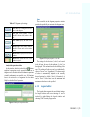
similar to the Postprocessor menu (See Figure 2.4).
The simulator’s analysis tools like Budget or Fluid
flux analyzer can be applied to the current time step of
the simulation, only, while the postprocessor also supports analyzing of time periods.
OO=ö=rëÉêÛë=j~åì~ä=J=m~êí=f
Figure 2.4 Comparison between Simulator Run and
Postprocessor menus.
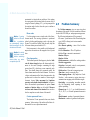
OKS=léíáçåë=jÉåì
OKS
léíáçåë=jÉåì
Many of the
items in this menu
have default values
that are suitable for
the novice user.
jÉëÜ=íêá~åÖìJ
ä~íáçå
This (default) setting selects triangular finite elements.
Three-nodal or 6nodal (currently not
supported) finite elements are implemented in 2D, and 6nodal or 15-nodal
(currently not supported)
prismatic
finite elements are
available in 3D.
jÉëÜ=èì~Çê~åÖìä~íáçå
selects quadrilateral finite elements. In 2D, you can
choose 4-nodal or 8-nodal finite elements. In 3D, the
choices are 8-nodal or 20-nodal prismatic finite elements.
sÉäçÅáíó=~ééêçñáã~íáçå=KKK
invokes the velocity-approximation options window
where a selection of different evaluation methods for
the computation of the local Darcy velocities is available.
`çåîÉÅíáîÉ=Ñçêã=íê~åëéçêí
applies the default transport equations. These equations are based on the continuity equation to eliminate
portions of convective terms, creating a natural dispersive-flux boundary condition. This option is recommended if mass transport can be formulated using firsttype boundary conditions and zero dispersive fluxes
along the remaining (outflowing) boundary sections.
aáîÉêÖÉåÅÉ=Ñçêã=íê~åëéçêí
invokes the divergence balance-improved formulation of the governing mass and heat transport equations. This formulation describes a total boundary flux
consisting of both convective and dispersive parts. This
option is recommended when modeling the total (net)
mass or heat flux along inflow boundary sections (e.g.
waste injection or leakages from a disposal site, see
Reference Manual for details).
fíÉê~íáîÉ=Éèì~íáçå=ëçäîÉêë
This (default) option is comprised of iterative equation system solvers that are used during the FEM computational process. The symmetric sparse flow
equations are commonly solved by a conjugate-gradient method using incomplete Gauss-based preconditioning. As an alternative, FEFLOW also offers the
algebraic multigrid SAMG solver (separate license
kçíáÅÉW= qÜÉ= ~äÖÉJ
required). SAMG has proven very powerful for diffiÄê~áÅ=
ãìäíáÖêáÇ
cult problems where the conjugate-gradient method
ëçäîÉê= p^jd= áë
takes a large number of iterations (poor convergence) ~î~áä~ÄäÉ= áå= cbcilt= Ñçê
êÉäÉ~ëÉ=RKN=~åÇ=ÜáÖÜÉêK=
or completely fails (divergence)1).
The asymmetric sparse transport equations can be
solved by a family of iterative techniques with incom1)
for more see White Papers Vol. III, Chapter 3
cbcilt=RKN=ö=OP
OK=pÜÉää=jÉåì
plete Crout-based preconditioning. The following solvers are available: Restarted ORTHOMIN, restarted
GMRES, CGS, BiCSTAB and BiCGSTABP. BiCGSTABP is the default iterative solver for asymmetric
problems. The iterative solvers are very effective and
reduce memory requirements. They are efficient for
solving large problems containing more than about
20,000 nodes. The maximum iteration number, available preconditioning method and the error criteria can
be changed by using the Properties dialogs.
lems (those with less than about 10,000 nodes). A
Gaussian profile solver is used for both flow and transport equations. The Reverse Cuthill McKee (RCM)
and, as an alternative, the Multilevel Nested Dissection
(MLNDS) nodal reordering schemes are incorporated
to minimize the matrix fill-in and the storage demand.
péÉÅáÑáÅ=çéíáçå=ëÉííáåÖë=KKK
opens a submenu for:
• Handling of the concentration and temperature
effects on fluid viscosity and density.
• Processing of multi-layered wells.
• Computation of the mass matrices.
• Quadrature rules to evaluate element integrals.
• Treatment of elements having fallen dry.
• Settings for unsaturated flow.
• Reverse flow field option.
For detailed information see online Help.
iÉÖÉåÇ=ÉÇáíçê=KKK
sets the properties for visualization of the modeling
results. Besides switching between linear, logarithmic,
or custom scales different resolutions are supported.
Customized legends can be saved and loaded again.
Figure 2.5 Iterative solver settings dialog.
aáêÉÅí=Éèì~íáçå=ëçäîÉê
The Direct equation solver is best for small probOQ=ö=rëÉêÛë=j~åì~ä=J=m~êí=f
^Ç~éíáîÉ=ãÉëÜ=êÉÑáåÉãÉåí=E^joF=
invokes automatic refining and derefining of the
finite-element mesh during simulation. The AMR is
based on an a posteriori error estimation for the spatial
discretization. It works currently only for 2D triangular
meshes.
p~îÉ=ÅìêêÉåí=ëÉííáåÖë
Important temporal parameters like file histories,
paths, solver settings, numerical options, personal
OKT=fcj=J=fåíÉêÑ~ÅÉ=j~å~ÖÉê
menu entries are saved immediately and FEFLOW will
start with these settings next time.
OKT
fcj=J=fåíÉêÑ~ÅÉ=j~å~ÖÉê
The Interface Manager controls the configuration of
the FEFLOW Programming interface. It allows the
linking of FEFLOW with third-party software or selfcreated code. Data can be exchanged for preprocessing,
during the simulation run and for postprocessing. The
interface allows to create additional submenus and
menu entries in the FEFLOW GUI, too. The IFM provides support in all phases of building and maintaining
user modules. An assistant guides the initial creation
process while the project management dispenses with
the need to edit Makefiles and others. A callback editor
generates the source code for each event you intend to
handle. Additional tools and editors complete the module-development environment. The modules are activated in the Add Modules menu of the Problem Editor
(see Section 5.13). Section 11 of this manual introduces
the Programming interface.
OKU
aáãÉåëáçå=jÉåì
This menu is used to select the dimensionality of the
finite-element formulation.
qïçJÇáãÉåëáçå~ä=EOaF
When the 2D toggle is activated, an areal, twodimensional representation of the study domain and
database is used. This default two-dimensional representation covers horizontal, vertical, and axisymmetric
models. If invoked for a three-dimensional model, it
will reduce the model (including the database) to a single 2D-sliced model representation.
qÜêÉÉJÇáãÉåëáçå~ä=EPaF
The 3D toggle is activated to employ three-dimensional modeling. If invoked for a two-dimensional
model, the model is extended a 3D (multi-aquifer or
multi-layer) volume. The extension of the model is
controlled by the 3D-Layer Configurator menu (Section 5.4). This menu immediately appears after the 3D
toggle is selected. The 3D-Layer Configurator menu
contains commands to configure the vertical extent of
the layer and the geometric relations for a 3D aquifer
system.
Figure 2.6 Interface manager (IFM).
cbcilt=RKN=ö=OR
OK=pÜÉää=jÉåì
OKV
qççäë=jÉåì
This menu has several submenus giving access to
useful programs integrated in FEFLOW.
pí~êí=Ûj~é=^ëëáëí~åíÛ=éêçÖê~ã=KKK
starts a program for georeferencing and rectifying
raster images.
pí~êí=Ûm~ê~ãÉíÉê=ÑáííáåÖÛ=éêçÖê~ã=KKK
starts the parameter fitting program FE-LM²
included with FEFLOW.
pí~êí=u=ïáåÇçï=Çìãé=KKK=
opens a small submenu to execute a window dump.
Menus or the display of the working window can be
dumped and saved in a .xwd file. Windows users may
prefer to add screen dumps to the clipboard by simply
hitting <Alt> + <Print Screen>.
iáÅÉåëÉ=ëÉíìé=KKK
allows to choose another license server or to add
and edit license information for FEFLOW. See the CDROM booklet for detailed information.
pí~êí=ÚuéäçíÛ=éêçÖê~ã=KKK=Erkfu=çåäóF
starts the XPLOT plotting program. XPLOT is an X
Window-based software tool supplementary to the
FEFLOW package. It works interactively to handle all
the plotting using the what-you-see-is-what-you-get
(WYSIWYG) principle. XPLOT works with the
XSPOOL program, another FEFLOW tool. These two
programs spool and queue all files directly to a plotter
within the UNIX network.
pí~êí=Ûmäçí=^ëëáëí~åíÛ=éêçÖê~ã=KKK=EtáåÇçïë=
çåäóF
invokes the sophisticated FEPLOT tool for composing and printing plots based on ESRI Shape files, DXF
files and FEFLOW plot files (See Section 6.4.2).
OS=ö=rëÉêÛë=j~åì~ä=J=m~êí=f
aáëâ=ëé~ÅÉ=KKK
displays a message window indicating the remaining hard-disk space in the partition containing the current working directory.
OKNM táåÇçï=jÉåì
This menu allows you to activate the Log messages and the
Time recording windows for the
simulation run. The Time recording window reports the CPU and
system times needed for each computational step during a simulation
run. Normally this option is not set as it is needed only
in specific cases. The Log messages window lists the
error messages and alerts of the program.
The Debug window replaces the UNIX console on
Windows systems for developing purposes. It is possi-
OKNN=fåÑç=jÉåì
ble to place messages in this window via interfacemanager commands (see Section 11).
OKNN fåÑç=jÉåì
This menu gives an overview over system
resources, problem specific information and provides
access to the top level of the online Help (Section Figure 2.7).
eÉäé
Help
invokes
the
FEFLOW online Help
pop-up window.
pÜçï=ÑáäÉ=KKK
shows (for viewing
only) a file to be
selected. The FEM output file *.dar is the default file
type.
píçê~ÖÉ=ÇÉã~åÇ=KKK
displays how much memory FEFLOW has allocated for the current model and how much memory
will be needed for performing the simulation.
mêÉëÉåí=éêçÄäÉã=ëìãã~êó
presents a summary indicating the progress of the
editing process. One important item is whether the current problem is ready to run. If it is not ready, you will
find hints how to complete the problem. You will also
see which parameters have already been user-specified
and which parameters have still default values.
cbcilt=RKN=ö=OT
OK=pÜÉää=jÉåì
^Äçìí
About opens the About FEFLOW pop-up window.
It includes copyrights, current version number, the date
of the last release, and a disclaimer.
Figure 2.7 Contents of the Info menu.
OU=ö=rëÉêÛë=j~åì~ä=J=m~êí=f
P
jÉëÜ=bÇáíçê=jÉåì=fíÉãë
P
=jÉëÜ=bÇáíçê=jÉåì=fíÉãë
PKN
fåíêçÇìÅíáçå
The Mesh editor is
a CAD-oriented tool
used to enter geometric data for a groundwater
flow
and
transport model. It is
the first menu you use
when creating a new
model.
Here
you
design the superelement mesh which represents the geometry
of the study area, i.e.,
the outer and inner
borders of the groundwater model. Superelements are the basis
for creating a finiteelement mesh.
The Mesh editor
contains tools to design the superelements. The number
of superelements can be arbitrary.
The Mesh editor is connected with the Mesh generator. The Mesh generator is used to interactively
mesh superelements with triangular or quadrilateral
finite elements. Type and form of the superelements
depend on the mesh type selected in the Options menu
of the Shell (Section 2.6).
If you use Mesh quadrangulation, you should note
that each superelement is automatically closed after the
fourth vertex has been set. For Mesh triangulation
(default), the superelement can have an arbitrary number of vertices, allowing a more complex design.
Superelements are drawn by mouse on a blank
screen or on a background map. The keyboard can be
used to specify exact coordinates. Meshes or patches of
superelements can be easily corrected and manipulated
by the following functions and utilities: Correct, Copy,
Zoom, Erase, Add, Shift, and Measure (for details, see
the subsections below). Context-sensitive messages
that appear in the message bar help you choose your
next step.
Start the Mesh editor:
To Create a New Design: From the Edit menu,
select Design superelement mesh .... This starts the
Mesh Editor with an empty working window.
For editing the mesh you can choose between the
cbcilt=RKN=ö=OV
PK=jÉëÜ=bÇáíçê=jÉåì=fíÉãë
mesh editor known up to release 4.8 and the so called
’New mesh editor’ which offers more comfortable and
more efficient tools for the superelement design.
To Work With an Existing Design: From the File
menu, select Load superelement mesh.... This loads a
previously designed superelement data file. You can
modify the design in the Mesh Editor or you can mesh
it by using the Mesh generator.
Online Help is always available by pressing the
Help button. Pushing the Exit to master menu button
returns you to the Master (Shell) menu.
PKO
kçíáÅÉW= fÑ= óçì= ìëÉ
ãÉëÜ=èì~Çê~åÖìä~J
íáçåI=É~ÅÜ=ëìéÉêÉäÉJ
ãÉåí=
Ü~ë=
íç=
ÄÉ
èì~Çêáä~íÉê~äK= qÜÉ= ëìéÉêÉäÉJ
ãÉåí=áë=~ìíçã~íáÅ~ääó=ÅäçëÉÇ
~ÑíÉê= ëéÉÅáÑóáåÖ= íÜÉ= ÑçêíÜ
îÉêíÉñK
kçíáÅÉW= lîÉêä~éJ
éáåÖ= ëìéÉêÉäÉãÉåíë
Å~ìëÉ= ~å= áåî~äáÇ
ãÉëÜ= ÖÉåÉê~íáçåK= tÜÉå
ìëáåÖ= íêá~åÖìä~ê= ãÉëÜÉëI
çîÉêä~ééáåÖ= çÑ= ëìéÉêÉäÉJ
ãÉåíë= áë= åçí= ~ìíçã~íáÅ~ääó
éêÉîÉåíÉÇK= _É= ëìêÉ= íç= ÅÜÉÅâ
óçìê= ëìéÉêÉäÉãÉåí= ãÉëÜ
~ÅÅçêÇáåÖäóK
PM=ö=rëÉêÛë=j~åì~ä=J=m~êí=f
kÉï=jÉëÜ=bÇáíçê
The new mesh editor offers many new
capabilities;
however, it does not yet
include every function available within
the old mesh editor.
Therefore, both editors are implemented
in
the
current
FEFLOW release.
^ÇÇ=éçäóÖçåë
This part of the mesh editor allows you to make
changes and additions to a superelement mesh. You can
place nodes and change lines to make them curved, circular or straight. For rough orientation the current coordinates of the mouse pointer are shown in the control
panel in the lower left corner of the window.
Press the left mouse button to fix a node. For exact
node positioning the Fixator
can be invoked by hitting
<F2>. It allows to explicitly enter values for the x
and y coordinates of the
Figure 3.1 Fixator.
node. Alternatively, a point
file can be loaded by opening the combo box. The
points are sorted according to their distance to the
mouse pointer. Selecting a point from the list, a new
node will be placed exactly at the point coordinates.
After the first superelement node is set, a rubber
line that can be dragged is attached to it. The next node
is fixed by mouse or keyboard in the same way as the
first. Nodes may be created in a clockwise or counterclockwise direction. Select the starting node again to
close a superelement. Before closing the superelement,
a recently set node can be clicked again to discard all
subsequent nodes. This action is indicated by the
cursor. To attach a new superelement to an existing one
click one of the existing nodes. Clicking on a superelement edge between vertices inserts a new vertex at the
current cursor position. This is indicated by the nodeinsertion cursor
.
During supermesh design it is possible to zoom in
and out with the zoomer and to pan the view clicking
the middle mouse button and dragging. You can use the
<TAB> and <SHIFT>+<TAB> keys for a gradual forward and backward panning, respectively.
PKO=kÉï=jÉëÜ=bÇáíçê
^ÇÇ=äáåÉ=~ÇÇJáåë=L=^ÇÇ=éçáåí=~ÇÇJáåë
Add-ins specify where nodes are to be set during the
finite-element mesh generation. They are very useful,
for example, to place nodes exactly at the locations of
wells and observation points, or for refining of zones
along rivers or faults. Add-ins are only applicable for
triangular meshes using the TMesh or the (external)
Triangle mesh generator (See Section 4.5). Add-ins are
designed in the same manner as superelement polygons.
To add a line add-in draw a line on the screen. The
method is identical to the Add polygons command. To
finish the drawing double-click the left mouse button.
The line can start or end inside or outside of the superelements. The parts lying outside of the superelement
mesh will be ignored during the mesh generation.
On each node of an add-in line a finite-element
node will be created during mesh generation. Options
for mesh refining along these lines are available (Section 4.5).
To add point add-ins draw points on the screen or
use the Fixator by hitting <F2>. On each point a finiteelement node will be created during the mesh generation. Options for mesh refining around these points are
available (Section 4.5).
Direct import of points or lines from background
maps is currently only supported by the old mesh editor
(Section 3.5).
qççäë=~åÇ=ëÉííáåÖë
The new mesh-editor tools and settings are listed in
Table 3.1. While most of them are self-explanatory,
some will be explained in more detail. The different
snapping functions allow an exact positioning of superelement nodes without having to explicitly enter the
coordinate values. In the ’Snap to raster nodes’ mode
the nodes are snapped to the nodes of a regular raster.
The raster distance can be set using the ’Editor properties’ button.
Table 3.1 Buttons of the New Mesh Editor
Undo
Unlimited undo memory
Redo
Unlimited redo memory
Move nodes
Mode to move single nodes
Select elements
Select elements by mouseclick
Delete
Delete selected elements
Snap to line
Snap nodes to lines
Snap to point
Snap nodes to points
Snap to
nodes
Snap nodes automatically to
(magnetic) raster
raster
Opaque/transparent
Switch display mode for superelements
Auto pan
Automatic panning while editing elements
Node info
Display node and element
number
Editor properties
Edit pan, snap, and raster
options
Alternatively, a background map loaded using the
map manager (Section 2.2) can be used as a template
for the superelement generation. Using ’Snap to’, the
active map can be selected for snapping. Set the corresponding buttons to snap superelement nodes to lines
cbcilt=RKN=ö=PN
PK=jÉëÜ=bÇáíçê=jÉåì=fíÉãë
and/or points of the background map. The snap distance can be changed within the ’Editor properties’
window.
Using the ’Move nodes’ mode you can correct your
superelements by dragging a node while pressing the
left mouse button. The Fixator is available by hitting
<F2> to specify exact coordinate values. To insert a
new node along the edge of an existing superelement,
click the left mouse button while the cursor shows the
node-insertion symbol
. To delete a selected node
hit the <DELETE> key. Snapping nodes together
closes gaps between different superelements. To separate connected superelements select a shared node and
hit <F5>. Curved boundary sections can be created by
dragging the middle node (smaller quadrilaterals) of a
superelement boundary line. Simultaneous hitting of
<F4> creates circular boundaries. Selecting the middle
node and hitting <F3> resets the curves to straight
lines.
The edge attributes (linear or parabolic) are saved to
the supermesh file.
dÉçíê~åëÑçêã~íáçå
FEFLOW provides an interface to different geographical transformation routines. FEFLOW comes by
default with an affine transformation algorithm in x-, yand z-directions. The corresponding input dialog
appears under the Transform mesh submenu of the
Mesh geometry menu. The target system and the
transformation parameters can be defined in a separate
dialog after clicking the Options button.
PO=ö=rëÉêÛë=j~åì~ä=J=m~êí=f
Figure 3.2 Mesh transformation dialog.
Additional methods, especially for Germany, are
available and can be licensed separately. Alternatively,
it is possible for each user to develop his own transformation routines. In case of need, contact WASY for
further information.
PKP
`çåíáåìÉ=mçäóÖçå=
aÉëáÖå
This part of the old Mesh editor allows you to
make changes and additions to a superelement mesh.
You can place nodes and change lines to make them
curved, circular or straight just as described for the new
mesh editor. However, there are some differences compared to the New Mesh Editor, e.g., it is not possible to
zoom or pan the mesh during the mesh-creation process.
PKQ=j~éW=få~ÅíáîÉL^ÅíáîÉ
PKQ
j~éW=få~ÅíáîÉL^ÅíáîÉ
This item allows to use background maps loaded by
the map manager (Section 2.2) as templates for the
polygon design. Once a file is selected its name is displayed in the “File:” text field. The map is activated by
setting the toggle to Active. During polygon design,
the cursor will then snap automatically to items of the
background map that are within snap distance. The
snap distance can be specified via the Snap button next
to the Insert button. By hitting the <F65> and <F6>
keys, the map can be made active and inactive, respectively.
PKR=
can import the corresponding objects all at once by
pressing the ’Add from map’ button.
bê~ëÉ=~ÇÇJáåë
This option works exactly like the “Erase superelements” (see Section 3.7) function of the Mesh Editor
menu.
eÉäé
Starts the FEFLOW Help Viewer for context-sensitive help.
`çåíáåìÉ=ãÉëÜ=ÇÉëáÖå
Returns to the Mesh Editor menu.
^ÇÇJfå=iáåÉëLmçáåíë
Clicking on the AddIn lines/points menu
item enters the Mesh
Add-in submenu. The
functionality of addins is described in
detail in Section 3.2.
The commands are
described briefly in
this section.
^ÇÇ=Ñêçã=ã~é
Imports lines or points from an activated background map:
Having activated a background map as described in
the last section the ’Add from map’ button becomes
enabled displaying ’Add lines from map’ or ’Add
points from map’ depending on the current setting. You
cbcilt=RKN=ö=PP
PK=jÉëÜ=bÇáíçê=jÉåì=fíÉãë
PKS=
`çéó=pìéÉêÉäÉãÉåíë
You can copy superelements by translation, rotation, or reflection. Copying can save you time and
allows to preserve some properties from one element to
the next. Several steps are necessary to copy a superelement. The Copy superelements editor will guide
you during the process.
Select a superelement or a
group of superelements with the
left mouse button. The selected
superelements are highlighted in
light blue on your screen (Figure). You can deselect an element by clicking it again.
Confirm the selection by clicking the right mouse
button.
A pop-up window (Figure 3.3) allows you to select
between the types of copying Copy by translation,
Copy by rotation, and Copy by reflection. Other options
in this menu are: Save original superelement, Delete
original superelement, and Pixel tolerance. This last
option allows you to merge superelements easily. Note
that in Figure 3.3 the default toggle buttons are set.
Follow the instructions for the type of copying you
have selected.
`çéó=Äó=íê~åëä~íáçå
Set two points (P1 and P2) for the translation vector.
`çéó=Äó=êçí~íáçå
Set the point of rotation axis. Type the angle in
degrees for a counterclockwise (positive values) or
clockwise (negative values) rotation.
PQ=ö=rëÉêÛë=j~åì~ä=J=m~êí=f
Figure 3.3 Copy superelements.
`çéó=Äó=êÉÑäÉÅíáçå
Set two points to mark the reflection line (nodal lassos are operating around marked nodes).
You can discard your newly created supermesh at
any time by hitting the <F2> key. Return to the first
step to repeat a copying procedure or to use a different
copy method. To exit the Copy superelements mode,
press the right mouse button.
PKT=bê~ëÉ=pìéÉêÉäÉãÉåíë
PKT=
bê~ëÉ=pìéÉêÉäÉãÉåíë
Superelements can be erased either individually or
collectively. Click on the Erase superelements button
and select one superelement or a group of superelements with the left mouse button. The selected superelements are highlighted in light blue on your screen.
Unselect a previously selected element by clicking it
again with the left mouse button. Confirm deleting of
the selection with the right mouse button. To undo the
erasing of a superelement or a group of superelements
hit the <F2> key. Exit by clicking the right mouse button.
PKU
mêçÄäÉã=jÉ~ëìêÉ
This menu allows to view and edit the dimensions
of the working window, the mesh, or the coordinates.
Be careful using this menu as the georeferencing of
your model is affected by these settings. For invoking
the menu click on the Problem measure button. A
pop-up window appears with the following options:
táÇíÜ=çÑ=ïçêâáåÖ=ïáåÇçï
Sets the width (in meters) of the working area. The
default value is 100 m.
sÉêíáÅ~ä=Éñ~ÖÖÉê~íáçå
Sets the vertical exaggeration of the working area.
The default ratio is 1:1 (no exaggeration).
local coordinate origin:
See Table 3.2 for a detailed description of the toolbar buttons.
Table 3.2 Buttons of the Shift Origin toolbar
Shift origin
Allows to interactively shift the
local origin. Move the cross
hairs by mouse to any point
inside or outside the model area.
Snap origin to
(X, Y) coordinates
Origin of local coordinates
snaps automatically to a point
selected by mouse-click.
Shift origin to
lower left corner
Shifts the origin of local coordinates to the lower left corner.
Shift origin to
lower right corner
Shifts the origin of local coordinates to the lower right corner.
Shift origin to
upper left corner
Shifts the origin of local coordinates to the upper left corner.
Shift origin to
upper right corner
Shifts the origin of local coordinates to the upper right corner.
Finish
Exit/close origin tool menu and
return to the Problem measure
menu.
pÜáÑí=çêáÖáå
Displays a toolbar for setting the location of the
cbcilt=RKN=ö=PR
PK=jÉëÜ=bÇáíçê=jÉåì=fíÉãë
d~ìëëJhêìÉÖÉê=ÅççêÇáå~íÉë=áåéìí
Allows to enter absolute Gauss-Krueger coordinate
values, xoGK and yoGK (in meters), for the origin of
the local coordinates. The default values are (0., 0.).
You can georeference the working window automatically by importing a background map for the model
area (See Section 2.2).
PKV
oÉëí~êí=jÉëÜ=bÇáíçê
This function should be used only if you wish to
discard what you have created with the Mesh editor.
Before restarting the mesh design, an alert box prompts
for a selection from the following options:
• Save the current superelement mesh in a file.
• Restart the editor from the beginning.
• Cancel (no restart).
PKNM pí~êí=jÉëÜ=dÉåÉê~íçê=
Clicking this button opens the Mesh generator.
The Mesh Generator, which meshes the superelements
with finite elements (quadrilaterals or triangles), is discussed in Section 4.
PS=ö=rëÉêÛë=j~åì~ä=J=m~êí=f
Q
jÉëÜ=dÉåÉê~íçê=jÉåì=fíÉãë
Q
=jÉëÜ=dÉåÉê~íçê=jÉåì=fíÉãë
QKN
local refinement and derefinement of the mesh.
fåíêçÇìÅíáçå
This section describes the generation
of
finite-element
meshes. It is assumed
that you have already
created one or more
superelements. During the simulation, results are computed on
each node of the finite-element
mesh
and
interpolated
within the finite elements. The denser the
mesh the better the
numerical accuracy,
and the higher the computational effort. Numerical difficulties can arise during the simulation if the mesh
contains too many highly distorted elements. Thus
some attention should be given to the proper design of
the finite-element mesh. To assist in creating a wellshaped mesh, FEFLOW offers various tools, including
QKO
dÉåÉê~íÉ=^ìíçã~íáÅ~ääó
A pop-up window allows you to enter the desired
total number of finite elements (default is 1000) for the
complete region of superelements.
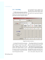
QKP
dÉåÉê~íÉ=^êÉ~ääó
Clicking on the Generate Areally button opens a
new pop-up window. If the Advancing-front mesh generator is selected (Section 4.5), you are asked to enter
the desired number of elements for each of the superelements. If you are using TMesh, Triangle or Transport mapping the Mesh density display/editor is
opened which allows you to set the number of elements
for each superelement.
The left part of the window shows the number of
elements which will be created for each superelement.
The generation is invoked by clicking the Start button.
(Re-)Compute element number distribution distributes a given total number of elements (default
cbcilt=RKN=ö=PT
QK=jÉëÜ=dÉåÉê~íçê=jÉåì=fíÉãë
1000) on the superelements. To change the number of
elements for a particular superelement click on the corresponding superelement number and type the new
value in the Edit number of elements line. If Autozooming is selected, the working window is automatically zoomed to the selected superelement.
Activating Area sorting changes the order of mesh
generation: Normally the mesh is generated in the same
order in which you have drawn the superelements. If
the Area sorting option is active, the mesh is generated
in the order of the superelement area, from the smallest
element to the largest one.
The triangulator can occasionally fail for an inappropriate subdivision of superelement edges. In this
case, the generator stops and an alert box presents different ways to continue. Your choices are:
• repeat the triangulation for the last superelement,
• start over from the beginning, or
• break the generation process.
Sometimes, a repeated generation for the same subdivision is successful, because the generator dynamically increases the number of iterations and allocates
larger working arrays.
Figure 4.1 Generate areally.
PU=ö=rëÉêÛë=j~åì~ä=J=m~êí=f
QKQ
dÉåÉê~íÉ=dê~Çì~ääó
Click on Generate gradually to start.
This option allows you to input the number of finite elements along each edge of
a superelement. The current superelement
edge is indicated by an arrow. Note that
for edges shared by two superelements
the number of elements has to be the same on both
sides. Therefore an input is required only once.
This function only works with the Transport mapping and Advancing front meshing methods as
described in Section 4.5.
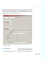
QKR
dÉåÉê~íçê=léíáçåë
The Generator options item defines rules for the
generation of the finite-element mesh.
FEFLOW implements three different mesh generators:
• Transport mapping for quadrilateral elements,
• Advancing front for triangular elements at superelement meshes without add-ins and
• TMesh (Delaunay) for triangular elements at
superelement meshes including add-ins.
Additionally, an interface is provided for the Triangle (Delaunay) generator for complex superelement
meshes including a large number of add-ins (copyright
by J. R. Shewchuk, University of California at Berkeley).
QKR=dÉåÉê~íçê=léíáçåë
Figure 4.2 Mesh generator options.
=qê~åëéçêí=ã~ééáåÖL~Çî~åÅáåÖ=Ñêçåí
Transport mapping creates quadrilateral finite elements while Advancing front is a mesh generator for
triangular finite elements. Having selected one of these
tools the menu displays the options as described below:
• Iteration number for triangular-mesh smoothing: Set the value higher if you want a better mesh
smoothing, but be aware that it might take much
more time, especially if the number of elements is
large. Only valid for Advancing front meshing.
• Triangulation based on quadrilateral supermesh elements: A triangle mesh will be generated
which is similar to a quadrilateral mesh where
each quadrilateral element is subdivided into two
triangles. With this option you get a very regular
distribution of finite elements. Only valid for
Advancing front meshing tool and quadrilateral
superelements.
• Automatic zooming during the areal and gradual meshing process: Automatically zooms to the
current supermesh element. The smallest superelement will be shown first.
qjÉëÜ=EaÉä~ìå~óF
This generator, developed at the EPFL-GEOLEP
Swiss Institute of Technology, Laboratory of Geology,
Lausanne, Switzerland, allows to comfortably define
the local variation of mesh density.
Having selected the TMesh meshing tool by clicking on the uppermost light blue button the following
menu items become visible:
• Level of refinement around superelement borders: Specify a refining factor for the finite element mesh along the superelement borders.
• Level of refinement around line/point add-ins:
If you have designed add-ins (Section 3.5) you
can define here how the mesh should be refined
along the lines and/or around the points.
kçíáÅÉW= jÉëÜ= ÖÉåJ
Éê~íáçå= Äó= qjÉëÜ
ïáíÜ= ãÉÇáìã= çê
ÜáÖÜ= êÉÑáåÉãÉåí= êÉèìáêÉë
ëáÖåáÑáÅ~åíäó=ãçêÉ=Åçãéìí~J
íáçå~ä=ÉÑÑçêí=~åÇ=~ÅÅçêÇáåÖäó
ãçêÉ= íáãÉ= Ñçê= íÜÉ= ãÉëÜáåÖ
éêçÅÉëëK
qêá~åÖäÉ=EaÉä~ìå~óF
The Triangle mesh generator, developed by J. R.
Shewchuk, provides a fast triangulation algorithm for
triangular meshes including a large number of add-ins.
Several options are available to control the meshing
process, which can be used individually or combined.
Most important are the following options: The Quality
cbcilt=RKN=ö=PV
QK=jÉëÜ=dÉåÉê~íçê=jÉåì=fíÉãë
Mesh (q-switch) option constrains the minimum angle
of the triangles. This angle can be directly prescribed.
Furthermore, using the L-switch option the triangulation can be forced to be a Delaunay for all triangles,
not just a constrained Delaunay. Commonly, the divide
and conquer Delaunay meshing algorithm is preferred. Alternatively, the i-switch option performs the
incremental Delaunay meshing algorithm.
QKS
kçíáÅÉW= råêÉëéçåJ
ëáîÉ= íçÖÖäÉë= áåÇáJ
Å~íÉ= íÜ~í= íÜÉ
ÅìêêÉåí= ãÉëÜáåÖ= çéíáçå
ÇçÉë= åçí= ~ééäó= íç= íÜáë= ÉäÉJ
ãÉåí=íóéÉK=qç=ÅÜ~åÖÉ=íç=~å
~ééêçéêá~íÉ= ÉäÉãÉåí= íóéÉI
ÅÜ~åÖÉ= íÜÉ= ÅçêêÉëéçåÇáåÖ
çéíáçå= áå= íÜÉ= pÜÉää= léíáçåë
ãÉåì= EpÉÅíáçå= OKSFK= SJ
åçÇÉÇ= íêá~åÖäÉë= ~åÇ= NRJ
åçÇÉ= éêáëãë= ~êÉ= ÅìêêÉåíäó
åçí=ëìééçêíÉÇK
pÉäÉÅí=bäÉãÉåíë
Before finite-element meshes can be generated, the
type of finite elements must be selected.
cáåáíÉ=ÉäÉãÉåí=ãÉëÜ=ëÉäÉÅíáçå
A current element library is shown when the Select
elements option is chosen. From this library, you may
select an element type for the FEM generation. Set the
corresponding toggle on the library submenu to specify
the element type you choose. Higher order elements (8nodal quadrilateral and 6-nodal triangle in 2D and 20nodal prism and 15-node prism in 3D) may lead to a
more accurate numerical result for the same number of
elements compared with linear element types, at the
expense of greater computational effort.
QKT
`çåíáåìÉ=jÉëÜ=aÉëáÖå
This option allows to return to the mesh-design process (described in Section 3) for further superelement
design or modification. If a finite-element mesh has
already been generated, a warning (alert) box appears
to ask you whether the generated mesh should be saved
(Save button), or discarded (Abandon button) before
entering the mesh editor again. Pushing the Cancel button closes the alert box without further action.
Figure 4.3 FEFLOW element library.
QM=ö=rëÉêÛë=j~åì~ä=J=m~êí=f
aÉÑ~ìäíë
Because defaults are available, the novice user may
skip this section. Defaults in 2D are the linear 4-nodal
quadrilateral element for the mesh quadrangulation
option, and the linear 3-nodal triangular element for the
mesh triangulation option. In 3D, the corresponding
defaults are the 8-nodal quadrilateral prism and the 6nodal triangular prism, respectively.
QKU=jÉëÜ=dÉçãÉíêó
jÉëÜ=ÉåêáÅÜãÉåí
Use the Mesh enrichment menu item to locally
refine or derefine a finite-element mesh. This can be
useful if local mesh refinements or improved mesh
accuracy are desired in areas where large gradients are
expected.
The enrichment can be executed using the mouse
alone or based on polygons or lines using the assigning
and joining techniques described in Section 5.6.
Figure 4.4 Alert box.
QKU
jÉëÜ=dÉçãÉíêó
Selecting this item invokes some tools for editing
the mesh.
aÉäÉíÉ=ÉäÉãÉåíë
The special option Delete elements may be useful
kçíáÅÉW= rëÉ= íÜÉ
whenever a mesh contains elements which should be
ÇÉäÉíáçå= ïáíÜ= Å~êÉ
íç= ~îçáÇ= ÛãìíáJ
excluded from the computation, for example, areas
ä~íÉÇÛ=
ãÉëÜÉëK= fåíÉêÅçåJ
having a negligible permeability. This approach is
åÉÅíÉÇ=ÄçìåÇ~êó=ÅçåÇáíáçåë
often better than assigning extremely small permeability values, which can lead to stiff and ill-conditioned Å~å=~äëç=Çáë~ééÉ~êK
matrix equations that are hard to solve.
qêá~åÖìä~êáò~íáçå=çÑ=èì~Çêáä~íÉê~ä=ãÉëÜÉë
This tool converts quadrilateral meshes to triangular
ones.
As indicated by the buttons you can subdivide one
quadrilateral element either into two or four triangles.
Splitting into two triangles can be performed using
either the shortest diagonal of each element or a consistent splitting direction. Applying the triangularization
results in very regularly meshed models.
oçí~íÉ=ãÉëÜ
This option allows to rotate a finite-element mesh in
the x-y plane. It is useful to align the domain to a given
gravity direction, for instance, with slope laws for
cbcilt=RKN=ö=QN
QK=jÉëÜ=dÉåÉê~íçê=jÉåì=fíÉãë
unsaturated or density-driven problems. After setting
the center point of the rotation either by mouse click or
using the Fixator by hitting <F2>, you are prompted for
the rotation angle. An alert box asks you to confirm or
discard the rotation.
jçîÉ=åçÇÉ
Use this option to move a single node of the finiteelement mesh. The moving operation is performed
either by clicking and dragging a node or by using the
Fixator. To invoke the Fixator click the node, keep the
left mouse button pressed and hit <F2>.
Node movement is also possible with background
maps where the nodes can be snapped to line or point
kçíáÅÉW=fí=áë=ÉåíáêÉäó data.
kçíáÅÉW= fÑ= ãçîáåÖ
åçÇÉë=áå=~=Pa=ãÉëÜ
íÜÉ= òJÅççêÇáå~íÉë
~êÉ= ~ìíçã~íáÅ~ääó= áåíÉêéçJ
ä~íÉÇ= ~ÅÅçêÇáåÖ= íç= íÜÉ= ëäáÅÉ
ÉäÉî~íáçåë=çÑ=íÜÉ=ãÉëÜK
äÉÖáíáã~íÉ= íç= ÅêÉ~íÉ
ãÉëÜÉë= Åçåí~áåáåÖ
áåíÉêáçê= ÜçäÉëI= ÉKÖKI= ïÜÉêÉ
~å=~èìáÑÉê=Åêçéë=çìíK
`ÜÉÅâ=éêçéÉêíáÉë
This button opens the Mesh property checker. Indicate all obtuse triangles shows all obtuse-angled elements in the mesh (triangles containing an angle
greater than 90°), which may cause numerical problems. You should change the supermesh and/or the
finite-element mesh to avoid such elements. To achieve
a better conformation of the finite-element mesh to the
problem and to reduce the number of obtuse-angled
elements, choose Node movement by Laplacian
operator on hydraulic head distribution. In order to
detect ill-connected superelements the option Count
number of interior holes can be helpful. Measure
total area and volume of the domain allows to calculate the complete area and volume of the model.
`êÉ~íÉ=ëìéÉêãÉëÜ=Ñêçã=KKK
The function ’Create supermesh from outer border
geometry’ allows saving of the outline of the finite element model as a new superelement mesh.
QO=ö=rëÉêÛë=j~åì~ä=J=m~êí=f
QKV
mêçÄäÉã=pìãã~êó
The Problem summary gives an overview about
the settings of the model. It can be invoked on different
levels in the FEFLOW pre- and postprocessing menus.
The following information will be presented:
• File name - specification of the file including data
type (ASCII or binary) and version number
• Problem title
• Most Recent updating - time of the last data
manipulation
• Problem Dimension - 2D or 3D problem
• Problem Type - saturated or unsaturated
• Number of layers
• Number of slices
• Problem measure - width of the working window
• Vertical exaggeration
• Projection - horizontal, vertical, or axisymmetric,
confined or unconfined aquifer
• Problem class - flow and/or transport process
• Time class - steady or unsteady flow
• Time-stepping scheme - fully implicit or CrankNicolson - with constant or varying time-steps automatic time stepping with different strategies
• Upwinding - no upwinding, streamline upwinding, full upwinding, shock capturing or least
square upwinding
• Element type - 4-, 8-, 3-, or 6-nodal elements in
2D, 8-, 20-, 6-, or 15-nodal prismatic elements in
3D,
• Mesh elements - number of generated elements
• Mesh nodes - number of generated nodal points
QKV=mêçÄäÉã=pìãã~êó
• Mesh optimization - indicates if nodal reordering
techniques have been performed (required for
direct equation solvers)
• Information about Flow boundaries, Flow initials and Flow materials - conditions already set
(you can determine whether initial and material
conditions have been set or remain at default
value, and whether boundary conditions are specified or unspecified.)
• Information about Transport boundaries, Transport initials and Transport materials - conditions already set (as above)
• Completeness of the current problem for running
the simulation - Yes/No
cbcilt=RKN=ö=QP
QK=jÉëÜ=dÉåÉê~íçê=jÉåì=fíÉãë
QQ=ö=rëÉêÛë=j~åì~ä=J=m~êí=f
R
mêçÄäÉã=bÇáíçê=jÉåì
R
The following main menus are available:
=mêçÄäÉã=bÇáíçê=jÉåì=
RKN
fåíêçÇìÅíáçå
While the Mesh
editor defines geometric
data,
the
Problem editor edits
all
remaining
attribute data such as
material properties or
initial and boundary
conditions.
The
Problem editor also
allows the definition
of the simulation type
and the editing of the
simulation-control
parameters.
mêçÄäÉã=Åä~ëë=
Serves for editing the title, general type of problem
(saturated or unsaturated media), problem class (steady
or transient flow or transport simulation), projection,
and the handling of free surfaces.
qÉãéçê~ä=C=Åçåíêçä=Ç~í~=
Sets parameters which control the simulation run
and offers input tools for time-varying data.
PaJpäáÅÉ=ÉäÉî~íáçå
Configures the vertical extent of the layer and the
geometric relations for a 3D aquifer system.
cäçï=Ç~í~
Provides submenus for the setting of all parameters
defining a subsurface flow problem (Section 5.5). It
also gives access to the editing menus for initial,
boundary, and material conditions.
qê~åëéçêí=Ç~í~
Offers a submenu structure similar to the Flow data
cbcilt=RKN=ö=QR
RK=mêçÄäÉã=bÇáíçê=jÉåì
menu for all parameters defining a contaminant mass
and/or heat transport problem.
oÉÑÉêÉåÅÉ=Ç~í~
Provides submenus to control the settings for comparison of measured and computed values.
fcj=ãçÇìäÉë
Controls which external program modules are used
within the current model. Please refer to Section 11 and
the online Help for detailed information concerning the
FEFLOW Programming Interface.
RKO
mêçÄäÉã=`ä~ëë
The Problem classifier dialog has three functions:
specifying the problem title, setting the problem class,
and specifying the problem projection. Refer to the
Reference manual for background information on
problem classes and projections. The current problem
title can be changed to a new project title, which will
appear in the data files.
The Problem measure (Section 3.8) menu, the
Mesh geometry editor (Section 4.8) and the Problem
summary (Section 4.9) were described in the previous
sections. In the following subsections, we discuss the
main properties of the editor in detail. Note that all
working steps within the menus can be carried out with
or without zooming.
Figure 5.1 Problem definition.
The General type of problem distinguishes between
the classical Saturated media (groundwater)
approach and Unsaturated or variably saturated
media.
QS=ö=rëÉêÛë=j~åì~ä=J=m~êí=f
RKO=mêçÄäÉã=`ä~ëë
A problem can have one of two distinct problem
classes:
• Flow only or
• Flow & mass/heat/thermohaline transport
Types of simulation in the Flow only class are
steady and transient flows. For unsaturated problems a
choice between the standard Richards equation and
steady-state linearization has to be made. Steady-state
linearization is an extremely fast solution method
whose applicability is restricted to special conditions.
For further information see online Help and the
FEFLOW White Paper ’Steade-state linearized Richards equation for fast solution of unsaturated flow systems (FUSY)’.
In the Flow & transport problem class, there are
three choices:
• steady flow and steady transport,
• steady flow and transient transport (default), or
• transient flow and transient transport.
Please note that in ’steady flow and transient transport’ mode only one iteration is performed for the flow.
That means that the initial conditions for flow have to
reflect steady state conditions!
Also, different cases of 2D problem projection can
be selected:
• horizontal (default),
• vertical, or
• axisymmetric problems.
Horizontal problems are aquifer-averaged flow and
transport processes, while vertical and axisymmetric
problems correspond to cross-sectional and meridional
models, respectively. Vertical and axisymmetric projections are the only available 2D projections for unsaturated media and for gravity-affected, fluid densitycoupled problems. 2D vertical or axisymmetric models
in saturated mode are always confined. To represent
free surface conditions an unsaturated simulation has to
be performed for such kind of models. Note that for
axisymmetric problems the axis of rotation corresponds to the vertical y-axis (where the x-coordinate is
zero).
For horizontal problem projection, optional toggle
buttons are available to switch between confined and
unconfined aquifers. Unconfined aquifers can either
have a ’free and movable’ top slice or be marked as
’phreatic’ where unsaturated flow is computed for dry
areas using a simplified approach. Note that an unconfined, free surface aquifer model leads to a nonlinear
problem formulation.
For three-dimensional saturated-flow problems with
free surfaces, an additional Free surface definition
menu is available for defining multiple free surfaces
and movable slices. For more detailed information
please see the FEFLOW online Help and the Tutorial
(Section 10.3.2.1).
The model can be transformed from a transient to a
steady-state model by changing the Type of simulation
in the Problem Class menu. If time-dependent boundaries, constraints or flow material exist, a special window appears where you can insert the steady-state time
step. The boundaries and parameters are interpolated
and then set constant.
cbcilt=RKN=ö=QT
RK=mêçÄäÉã=bÇáíçê=jÉåì
RKP
qÉãéçê~ä=C=`çåíêçä=a~í~=
jÉåì
Essential parameters that control the stability and
accuracy of the simulation are defined here. The
parameters include: number of time steps, type of time
stepping, final time, level to switch to Crank-Nicholson
(CN) higher-order scheme, error tolerance and convergence criteria, types of upwinding, and nature of the
time-varying functions.
Figure 5.2 Temporal & control data.
QU=ö=rëÉêÛë=j~åì~ä=J=m~êí=f
qáãÉ=ëíÉéë
Transient simulations require temporal discretization. You can choose between Constant time steps,
Varying time steps, and Automatic time step control.
This last choice also allows to you select between different adaptive schemes. For constant time steps, the
default setting is 1 day. Note that time steps are not
applicable for steady-state problems.
Constant time steps usually reduce the numerical
effort during the simulation because the simulator can
use efficient resolution techniques. This avoids updating the matrix system for linear problems in a time-step
marching process.
Varying time steps can be entered directly in a
Time-step editor, or may be imported from a database.
The Automatic time-step control can be performed using either the Forward Euler/backward
Euler (FE/BE) time-integration scheme, which is 1st
order in time (often appropriate for density-driven and
unsaturated problems), or the Forward Adams-Bashforth/backward trapezoid (AB/TR) time-integration
scheme, which is 2nd order in time. For variably saturated problems the Aggressive target-based timemarching scheme, either fully implicit or semiimplicit, may provide an effective solution strategy.
Pushing the button Specific options for time step
control schemes, constraints and specific options for
the automatic time-stepping process can be set.
iÉîÉä=íç=ëïáíÅÜ=íç=`kJëÅÜÉãÉ
Sets the level to switch to Crank-Nicolson (CN)
higher-order scheme (not applicable to automatic timestep control). The default is 2000. This means that up
to the 2000th time step, a standard, fully implicit timestepping scheme with first-order accuracy is used. Subsequently, the second-order accurate CN scheme is
RKP=qÉãéçê~ä=C=`çåíêçä=a~í~=jÉåì
employed. While the implicit scheme is unconditionally stable, the CN-scheme can cause oscillations. Set
the level to zero to use the CN-scheme from the beginning.
bêêçê=~åÇ=ÅçåîÉêÖÉåÅÉ=ÅêáíÉêá~
The Error tolerance controls termination of the
iterative procedure for both nonlinear density-coupled
flow and transport, nonlinear processes in unconfined
aquifers and nonlinear flows for unsaturated media.
Note that the error is dimensionless. Its default value is
0.001. The parameter has no meaning for linear (e.g.,
horizontal and/or confined) problems. Setting a smaller
values enforces higher accuracy and implies increased
numerical effort, i.e., more iterations before termination. The error norms are defined as follows:
The Euclidean L2 integral root mean square
(RMS) error norm is the default error norm to measure
an integral error quantity. The Absolute L1 integral
error norm represents an average of absolute deviations
of the error in the solution domain. The Maximum L ∞
error norm can be useful to focus on the maximum
error occurring in the solution. It is the strongest measure and should be used if the local error is important in
the numerical process (’scheme listens to each sound’).
Modify the setting of the Maximal number of iterations per time step for problems which need many
iterations to meet the convergence criterion. If the error
does not fall below the criterion during the given number of iterations an error message is produced in the
Log window.
Adaptive mesh error and the A posteriori error
estimator define the computation of the Adaptive
mesh refinement (See Section 2.6).
Refer to the White Paper ’Error norms used in
FEFLOW’ (Chapter 5 of the White Papers Vol. I) for
additional information.
réïáåÇáåÖ
Five types of Upwinding settings are available to
stabilize numerical results for mass and heat transport
problems:
No upwinding (Galerkin-FEM approach) This is
the default option and produces the best accuracy;
however, it may lead to oscillations in the concentration or temperature results if convection-dominated
transport processes are modelled on coarse meshes.
Streamline upwinding is recommended if oscillating results have been produced. It stabilizes the computation by introducing a streamlined damping measure
(numerical dispersion).
Full upwinding remains the last resort for damping
oscillations, if all other types have failed. However, it
can generate a great amount of numerical dispersion.
Shock capturing adds a nonlinear anisotropic
damping factor to stabilize convection-dominant transport processes. This powerful method removes numerical oscillations at abrupt changes or fronts of the
solution with a minimal amount of numerical dispersion. It is only available for adaptive time-stepping
schemes.
Least-square upwinding represents an alternative
kçíáÅÉW= cçê= ÑìêíÜÉê
numerical scheme to solve transient advection-disperáåÑçêã~íáçå=êÉÑÉê=íç
sion transport problems. In contrast to standard techíÜÉ= cbcilt= tÜáíÉ
niques it leads to symmetric matrix systems and m~éÉê= ÛqÜÉ= mÉíêçîJd~äÉêâáå
possesses a built-in streamline-like upwind characteris- äÉ~ëí= ëèì~êÉ= ãÉíÜçÇ
EmdipFÛK
tics.
aáêÉÅíáçå=çÑ=Öê~îáíó
Use this option to change the direction of the gravity vector for the model.
cbcilt=RKN=ö=QV
RK=mêçÄäÉã=bÇáíçê=jÉåì
péÉÅáÑáÅ=çéíáçå=ëÉííáåÖë
Offers access to special numeric settings. You can
enter the same menu from the shell Options menu (see
Section 2.6).
RKPKN
bÇáí= íáãÉJî~êóáåÖ= éçïÉê= ÑìåÅJ
íáçåë
Invokes the Power function editor, in which you
can edit time-related functions interactively.
An unlimited number of power functions can be
created, edited, imported, and exported. The edited
power function is displayed automatically as a time-
value plot. Power functions are used for time-varying
functions such as varying time-steps (this chapter),
time-varying boundary conditions or material parameters. Each power function is identified by an integer ID.
These IDs are listed in the Flow data menus and can be
assigned directly or interpolated on the mesh as boundary conditions, constraints or material parameters. To
each function you can add a comment, e.g., the name of
an associated well.
There are different types for the curves:
• Polyline: the value pairs (time/function values) are
connected by linear interpolation.
Figure 5.3 Time-varying power functions editor.
RM=ö=rëÉêÛë=j~åì~ä=J=m~êí=f
RKP=qÉãéçê~ä=C=`çåíêçä=a~í~=jÉåì
• Constant: the function values define a stepwise
constant function. For the ramp steepness an internal value of 89.994° is used.
• Akima uses a third-order polygonal smoothing
based on the given values.
• Akima2 smooths the function using additional
middle nodes.
Each function can be applied in one of two time
modes:
• non-cyclic
• cyclic
In non-cyclic mode the function value is held constant after the simulation time has reached the last time
value defined in the time-varying function. In cyclic
mode the function is applied again from its beginning
and until the simulation ends. Use this mode to apply,
for example, annual hydrographs in a multi-year simulation.
RKPKO
iáëí=íáãÉJêÉä~íÉÇ=ã~íÉêá~ä=Ç~í~
In FEFLOW all material data can vary over space
and time. The data are assigned via the T-List tool or
the Join tool in the Material data menus of the Flow
data and Transport data options (Section 5.5 and Section 5.9).
The submenu termed Material data time list menu
displays, for each material parameter, the time values
for which material distributions are defined. During the
simulation, the current value is obtained by interpolating between these given time steps, either linearly
(‘Polylined’) or using a third-order polygonal smoothing (‘Akima’).
Time-related material data can be applied in linear
Figure 5.4 Material data time list controller.
(non-cyclic) or cyclic mode (see Section 5.3.1).
Time-related material data is stored either in the
problem file (*.fem) or in an external ASCII or binary
file (*.mli). Specify the name of the external file in the
input field.
The Preview time dependency button opens a plot
window for the time-varying data for each element in a
diagram.
Figure 5.5 Preview time dependency of material data.
To delete the entire material list push the Delete list
for material button.
cbcilt=RKN=ö=RN
RK=mêçÄäÉã=bÇáíçê=jÉåì
RKQ
Pa=päáÅÉ=bäÉî~íáçå
This submenu allows you to define, control, and
plot the elevations of the single slices in a 3D problem.
Use the z-coordinates button to assign the elevations to the nodes. Besides the ’Global’ and ’Nodal’
mode a linear interpolation method (’Skew plane’) and
different regionalization methods for imported data
(’Database’) are available.
Click Reconfigure 3D task to enter the Layer configurator window. The Layer configurator allows you
to visualize and modify the different layers and slices
and their elevations in a 3D model (see Section 10.4.2).
To avoid intersection of slices during the assigning
of z-elevations a minimal slice distance can be defined
in the Slice distance modifier.
Figure 5.6 Slice distance modifier.
For more detailed explanations see FEFLOW online
Help.
RKR
cäçï=a~í~
Initial conditions, boundary conditions, and flow
material parameters can be displayed and edited.
Pushing the Flow data button in the Problem Editor
menu invokes the Flow data submenu.
The first item, Flow initials, opens a submenu for
assigning and viewing the initial hydraulic head conditions. More information about this item is available in
Section 5.6.
The Flow boundaries option enables
you to edit first-, second-,
third-,
and
fourth-type boundary
conditions and constraints in a separate
submenu. Parameter values can be entered either
graphically using the ’Nodal’, ’Border’ and ’Rubberbox’ options or by different 1D and 2D ’Database’
interpolation methods. Both stationary and time-varying boundary conditions can be assigned. The definition of constraints for the boundary conditions is
executed via submenus.
The Flow materials option displays a submenu for
editing all material parameters necessary to desribe a
saturated or unsaturated flow problem. Parameter values can be set globally or locally. Local stationary or
time-varying values can be assigned elementwise, by
using a template, by kriging and Akima interpolation,
or by extrapolation from databases.
RKS
cäçï=fåáíá~äë
When Flow initials is selected from the Flow data
RO=ö=rëÉêÛë=j~åì~ä=J=m~êí=f
RKS=cäçï=fåáíá~äë
menu, a submenu appears to specify initial conditions
for flow. The following interactive, mouse-supported
tools are available to enter, edit, and plot flow initials:
Items
Items
Tools’ options
Mesh inspector
Tools
Return
Keyboard request box
Figure 5.7 Flow Initials submenu.
^ëëáÖå
Manages the keyboard-controlled and mouse-based
input of data and regionalization from databases.
Choose from the following input types:
• Global - Uniform value for the whole model (2D)
or the current slice (3D),
• Nodal - Specific value for mouse-selected single
nodes,
• Elemental - Specific value for mouse-selected
single elements,
• Rubberbox - Uniform value for an area marked
by a rubber box,
• Database - Values from a database by regionalization (Figure 5.8). The databases can be ESRI
Shape files, dBASE files or ASCII databases.
Using ASCII databases you have to select the
appropriate columns for the (x, y)-coordinates and
for the function value, or the data have to be prepared as so-called triplet files using the format: xcoord. y-coord. function-value.
In the Flow initials menu you can regionalize stationary data only, where the function value describes
the constant value. In the Flow boundaries and Flow
materials menus transient data can be regionalized, too.
For examples please refer to the Demonstration Exercise book and the Tutorial (Section 10), or invoke the
FEFLOW online Help hitting <F1>.
`çéó
Is mostly used for 3D problems. It copies flow initial data from the current slice to other slices. Do not
forget to assign flow initials to each slice, not just the
top one! The Advanced option allows copying of an
initial distribution to a reference distribution with a
given identifier. Reference distributions can be used as
a placeholder for data (see Section 5.10). For a detailed
description of the different options see the online Help.
cbcilt=RKN=ö=RP
RK=mêçÄäÉã=bÇáíçê=jÉåì
Figure 5.8 Database regionalization window and column Selection.
gçáå
Allows you to use ASCII or Shape file polygons, or
FEFLOW supermeshes, as templates. You can interactively set values for each subarea, interpolate triplet
files on selected subareas or import a value for each
subarea automatically by linking the ID of the subarea
with a column of an Arc/Info, ASCII or a dBase database. It is also possible to assign values from a database
to different timesteps of time-varying material data (see
Section 10.3.4.3).
The linking of a polygon file with a database is supported by a submenu.
See the online Help for detailed information and
have a look at the application example of the FEFLOW
Tutorial (Section 10.3.2.2).
RQ=ö=rëÉêÛë=j~åì~ä=J=m~êí=f
Figure 5.9 Linking of database with spatial data file.
RKS=cäçï=fåáíá~äë
aÉÄìÖ
Displays and modifies data groups. Data ranges or
subareas of the model domain (via background maps)
can be selected and the corresponding values can be
changed by adding/subtracting, multiplying/dividing,
or simple replacing operations.
pÜçï
Plots the flow initials as colored fringes (Figure
5.10).
s~åáëÜ
Switches off the Show option.
péÉÅá~ä
Allows data visualization and export via the Data
store manager (DSM), which is available from other
menus, too. The DSM manages the import and export
of spatial data in predefined or user-defined file formats that can be linked with attribute data. See online
Help for more information. The Special menu also
allows to compute ‘Head minus bottom’ and ‘Top
minus Head’ isoline-maps.
Figure 5.10 Special menu.
cbcilt=RKN=ö=RR
RK=mêçÄäÉã=bÇáíçê=jÉåì
jÉëÜ=fåëéÉÅíçê
Displays the current value and
physical units for the node in the
Inspector magnifier. If an ESRI shape
file has been loaded, its attribute values are listed in a
second Database inspector window (Figure 5.11).
`çåíÉåí=~å~äóòÉê
Offers functionality for computing the fluid/mass/
energy content of the model. There are eight different
contents to evaluate. They are listed in Table 5.1.
Table 5.1 Content analyzer options
Total volume [m³]
Void volume [m³]
Fluid content [m³]
Diluted mass (fluid phase) [g]
Sorbed mass (solid phase) [g]
Figure 5.11 Mesh Inspector echo.
hÉóÄç~êÇ=êÉèìÉëí=Äçñ
Accepts keyboard input. Having selected an option
of a tool which requires keyboard input a default entry
is shown here. To change the value click into the box,
select the default value with the mouse in order to
replace it or hit the <TAB> key. Below the box the
physical unit of the input value is displayed.
Figure 5.12 Keyboard request box.
oÉíìêå
Click this button to return to the upper menu level.
RS=ö=rëÉêÛë=j~åì~ä=J=m~êí=f
Energy of fluid phase [J]
Energy of solid phase [J]
Total energy content [J]
The content analyzer is provided in all three (flow,
mass and heat transport) initial-value menus as well as
in the simulator and the postprocessor menus.
RKT
cäçï=_çìåÇ~êáÉë
The Flow boundaries menu supports the input of
the boundary conditions for the flow equations. Boundary conditions can be stationary or time-varying. All
RKT=cäçï=_çìåÇ~êáÉë
boundary conditions can be limited by Constraints. A
detailed description of the different types of boundary
conditions is given in the Reference Manual. The
boundary conditions are:
• Head (first type, Dirichlet, [m]): It describes a
fixed potential at a node.
• Flux (second type, Neumann, [m/d], [m²/d]):
Assigns a flux to a node, for a 2D horizontal confined model the flux is considered depth-integrated. The boundary condition is only valid if
you define a distance over which it should apply
by selecting adjacent nodes.
• Transfer (reference hydraulic head, third type,
Cauchy, [m]): Defines a reference hydraulic head
of a domain outside the model such as a river or a
lake. The boundary condition is only valid if you
define a segment along which it should apply by
selecting adjacent nodes. You have to define a
Transfer rate in the Flow materials menu (Section 5.8) for the leakage arising between this reference hydraulic head and the aquifer.
• Well (fourth type, [m3/d]): Describes the injection or withdrawal of water at a single node.
It is possible to constrain the boundary conditions
by setting Constraints. The Constraint conditions of
Flow boundaries submenu is opened by clicking the
arrow to the right of each boundary condition button.
Figure 5.13 Boundary and constraint conditions menus.
You can limit a potential boundary condition by
maximum and minimum bounds for flux, or a flux
boundary condition by maximum and minimum values
for the resulting hydraulic head. Transfer boundary
conditions can be limited either by head or by flux,
while well boundaries are constrained by head. Furthermore, all constraints can be edited as time-varying
functions.
For a better understanding of these options please
refer to the Demonstration Exercise and the Tutorial
section.
Boundary and constraint conditions will be displayed as symbols on the nodes and can be checked by
using the Mesh inspector. A second window, the
Database inspector displays the properties of the
background map, if present (ESRI shape file).
We recommend to read the corresponding section in
kçíáÅÉW= cçê= ÑìêíÜÉê
áåÑçêã~íáçå= ~Äçìí
íÜÉ= ÜÉ~Ç= ÅçåJ
ëíê~áåí= Ñçê= PêÇJâáåÇ= ÄçìåÇJ
~êó= ÅçåÇáíáçåë= êÉÑÉê= íç= íÜÉ
tÜáíÉ= m~éÉê= ÛbñíÉåÇÉÇ= ÑçêJ
ãìä~íáçåë= çÑ= Åçåëíê~áåíë= Ñçê
`~ìÅÜóJíóéÉ= EPêÇ= âáåÇF
ÄçìåÇ~êó= ÅçåÇáíáçåë= áå
cbciltÛK
kçíáÅÉW= lìíÑäìñÉë
~êÉ=ÇÉÑáåÉÇ=~ë=éçëáJ
íáîÉ= Ñçê= ÄçìåÇ~êó
ÅçåÇáíáçåëK= eçïÉîÉêI= Ñçê
Åçåëíê~áåí= ÅçåÇáíáçåë= íÜÉ
ÇÉÑáåáíáçå= áë= çééçëáíÉI= ÜÉêÉ
áåÑäìñÉë=~êÉ=éçëáíáîÉ>=
cbcilt=RKN=ö=RT
RK=mêçÄäÉã=bÇáíçê=jÉåì
Figure 5.14 Mesh inspector.
the Reference Manual and to use the online Help.
In addition to the standard commands of the Flow
data menus, the Flow boundaries menu offers the following tools and functions:
bê~ëáåÖ
Deletes some or
all of the boundary
conditions via a cascade pop-up menu.
First-,
second-,
third-, or fourthtype, or all boundary conditions can be erased from the
current slice. Use the right mouse button to confirm
and execute. Note that a value-related erasing can be
performed using the Debug tool (see Section 5.6).
qáãÉJî~êóáåÖ=ÑìåÅíáçå=faë
Controls assigning of time-varying boundary conditions by assigning power functions. Click on Timevarying function IDs for opening the Power Functions editor (which you can also enter from the TemRU=ö=rëÉêÛë=j~åì~ä=J=m~êí=f
poral & control data menu, Section 5.3.1). A slider
bar below the button contains the ID numbers of the
currently defined time functions. For any ID shown,
the respective toggle can be set to assign the respective
function to a time-varying boundary condition.
The
left-most
toggle
(default setting) corresponds to time-constant
boundary
conditions.
Before assigning boundary conditions, you should set
the corresponding ID toggle. For time-varying functions, the symbol of the boundary conditions is shown
together with the corresponding ID number while stationary boundary conditions are indicated by symbols
without an ID number.
^ëëáÖå
Is similar to the Assign tool in the Flow Initials
menu (Section 5.6), with one additional option: Border
is a mouse-controlled input of boundary conditions
along the boundaries of the model. A constant value
can be set, or, by setting a start and an end value, a linear interpolation along the boundary is performed. The
Database option supports here also the 2D regionalization of time-varying boundary conditions and the direct
assignment of database values on the nodes. The latter
option is useful to import boundary conditions
exported from another FEFLOW model using a similar
mesh. For time-varying interpolation the triplet files
must contain the ID of a Power function as function
values (format of a triplet file: x-coordinate y-coordinate function-value). See the FEFLOW online Help for
detailed instructions.
RKU=cäçï=j~íÉêá~äë
gçáå
In addition to the basis functionality described in
Section 5.6, the Join tool supports the 1D regionalization of stationary and time-varying data along lines, for
example, for modeling river systems as boundary conditions, and 2D regionalization of time-varying data.
The joining can either be performed interactively or
automatically for all lines. The line order for joining
can be selected based on the order in the line file or
based on the order of an arbitrary database column.
bñéçêí
Exports the boundary conditions as ASCII files.
léíáçåë
Are only important for flux and transfer boundary
conditions in a certain context. Values of flux and
transfer can be treated as area-independent, which
means that the discharge varies with the cross-sectional
area of the effective aquifer, or treated as depth-integrated where a varying cross-sectional area does not
affect the quantity of the discharge. For unsaturated
flow the flux boundary condition can differ between
flux-type and gradient-type conditions. The latter is
useful to formulate free drainage boundary conditions.
`çåîÉêí
Changes type and attributes of boundary conditions,
for example, you can convert flux boundaries to transfer boundaries. Note that the values remain constant
but the units change.
RKU
cäçï=j~íÉêá~äë=
The submenu items explained in this section are
used to enter the material conditions for the flow equations. The specific material requirements depend on the
problem dimensionality and projection type for 2D
problems (horizontal, vertical, axisymmetric) as
selected in the Problem class menu. Note that these
items imply different meanings for the Tools button,
which can be set either to Assign, Join, Copy, Show,
Vanish, Debug, T-List, Special or Options. The Assign
tool is the default. It allows the assignment of materialparameter values necessary for describing the selected
problem type. For more detailed information about
these tools see Section 5.6.
The required physical units of each material parameter are
indicated in the Keyboard request box. The input follows the same steps
as outlined above for initial conditions.
In addition to the standard Flow data tools described
in Section 5.6, the following tools are available:
^ëëáÖå
Time-dependent material data can be regionalized
using the ’Database’ option either from power functions at specified locations or from a database containing the values for each time step in a column. See
online help for a detailed description.
qJiáëí
Controls the creation of time-varying material distributions. The Assign current distribution option
assigns the current material distribution to a time entry,
Copy list data copies time varying data between layers
cbcilt=RKN=ö=RV
RK=mêçÄäÉã=bÇáíçê=jÉåì
and different parameters. Preview time dependency
plots a diagram for each element. This can also be done
in the Temporal & control data menu (Section 5.3).
the corresponding parameters.
Figure 5.15 Material data time list editor.
léíáçåë
Define here if the anisotropy of the conductivity
should be oriented to Cartesian coordinate system or to
the layer inclination.
`çéó
Copy time-varying material-parameter values
between layers or to another material parameter
(Advanced option).
råë~íìê~íÉÇ=éêçéÉêíáÉë
The item Unsaturated properties switches to the
input menu for unsaturated-flow material parameters.
Use this menu to choose between Van Genuchten,
Brooks-Corey, VG modified, Haverkamp, Exponential and Linear parametric relationships and to assign
SM=ö=rëÉêÛë=j~åì~ä=J=m~êí=f
Figure 5.16 Unsaturated properties.
The default setting for the whole model domain is
the Van Genuchten relationship. To change the parametric relationship for parts or all of the model, set the
switch to the new relation, choose one of the input
tools, e.g., assign or join, and click the model button. It
is possible to use different parametric relations for different areas within one model.
Use the Porosity button to assign matrix porosity
for unsaturated conditions.
The white box displays the equations corresponding
to the active parametric relationship. The parameters to
be assigned are enclosed in red boxes. To set a parameter choose any input tool and click the symbol of the
parameter in the equation.
Set the
button to incorporate capil-
RKU=cäçï=j~íÉêá~äë
lary hysteresis in a simulation. Use the switch to
change between the wetting curve and the drying
curve.
The Inspected as line specifies the behavior of the
mesh inspector. Choose between viewing saturation vs.
capillary head and saturation vs. conductivity Curves
or the Values in text mode. nd1 and nd2 determine the
resolution of the curves while min ψ prescribes the
minimum capillary head for the curve.
Click the Saturated properties button to return to
the Flow Materials menu.
See the FEFLOW online Help for additional information.
In the following Table 5.2 all parameters for saturated and unsaturated flow are listed.
Table 5.2 Flow materials
Parameter
Description
Application
SATURATED MEDIA
Conductivity
Proportional to flow resistance in an aquifer
Transmissivity
Proportional to flow resistance and aquifer thickness
Anisotropy factor
Anisotropy angle
Ratio of maximum directional value to its original value
Angle between cartesian x-axis and major direction of
anisotropy
Bottom elevation for elements
Top elevation for elements
Drain/fillable void space in aquifer
Mass buoyant expansion coefficient for density coupled
flow
Heat buoyant expansion coefficient for density coupled
flow
Tendency of void space to be reduced under pressure
Aquifer bottom elevation
Aquifer top elevation
Storativity
Density ratio
Expansion coefficient
Storage
compressibility
In-/outflow on top/bottom
Source/Sink
Transfer rate in/out
Spatially variable recharge/evaporation on top or bottom slice
Spatially variable recharge/evaporation
Value computed from conductivity and thickness of colmation layer (“leakage coefficient”)
Major principal direction
2D horizontal, confined
2D
2D
2D horizontal
2D horizontal
Unconfined aquifer
2D vertical and 3D
modeling
2D vertical and 3D
modeling
3D
2D
Required for Transfer
boundary conditions
cbcilt=RKN=ö=SN
RK=mêçÄäÉã=bÇáíçê=jÉåì
Table 5.2 Flow materials (continued)
Parameter
Description
UNSATURATED MEDIA
Ss
Maximum saturation
Sr
Residual saturation
Ψa
Air entry pressure
Porosity
n, A, B, α , β , δ
Total porosity
Fitting parameters for the different parametric models
below
Parametric model for unsaturated flow
Parametric model for unsaturated flow
Parametric model for unsaturated flow
Parametric model for unsaturated flow
Parametric model for unsaturated flow
Parametric model for unsaturated flow
Van Genuchten
Brooks-Corey
Van Genuchten (VG) modified
Haverkamp
Exponential
Linear
SO=ö=rëÉêÛë=j~åì~ä=J=m~êí=f
Application
RKV=qê~åëéçêí=a~í~
RKV
qê~åëéçêí=a~í~=
In this section, initial conditions, boundary conditions, and transport material properties for both contaminant mass and heat are specified. Due to the
similarity between the parameters for contaminant
mass transport and for heat transport, only the contaminant mass transport menus will be described explicitly.
For detailed information about the principles and basic
equations of transport modeling please refer to the Reference Manual.
Many of the procedures are the same as
those in Section 5.5,
which is referred to frequently in this section.
The Transport initials
menu offers not only the
setting of an initial distribution of the mass concentration but also the
possibility to define a reference
contamination
mass/temperature, which
is used for the calculation of the fluid density. For
detailed information refer to the FEFLOW online
Help (hit <F1> in the Transport initials menu) or the
Reference Manual The Transport boundaries menu
is similar to the Flow boundaries (Section 5.7) menu.
For the definition of the mass boundaries we again
refer to the Reference Manual. The Transport materials menu differs in the parameters from the Flow materials menu. The tables in the Reference Manual give
the default units for the transport parameters, and the
online Help gives more detailed information. You can
assign, edit, and debug transport initials, transport
boundaries and transport materials. The Mass transport materials menu allows you to set the following
parameters: Aquifer thickness, Porosity, Sorption
laws (Henry, Freundlich, Langmuir) and Coefficients,
Molecular diffusion, Longitudinal dispersivity,
Transverse dispersivity, Dispersion type (Linear,
Nonlinear), Decay types (First Order, MichaelisMenten, Decay Chains) and Rate coefficients of reaction kinetics, Transfer rate, and Source/sink of contaminants.
The Heat transport data menus are similar to the
Mass transport data menus. For an explanation of the
parameters, see the Reference Manual.
RKVKN
qê~åëéçêí=áåáíá~äë
The initial mass
concentration (temperature) can be entered
globally, element-wise,
or node-wise. Reference mass concentration and/or Reference
temperature can be
defined for to take into
account the influence of
viscosity and density on
the effective permeability. See Section 5.6 for
an overview of how data can be viewed, assigned, and
edited. You can also find a description of the Content
Analyzer there. For detailed information see the online
Help.
cbcilt=RKN=ö=SP
RK=mêçÄäÉã=bÇáíçê=jÉåì
RKVKO
kçíáÅÉW= qÜÉ= ÅçåJ
ÅÉéíì~ä= ÇÉëáÖå= áë
ëáãáä~ê= Ñçê= ~ää= cäçï
~åÇ=qê~åëéçêí=a~í~=ãÉåìëK
oÉÑÉê= íç= íÜÉ= cäçï= fåáíá~ä
a~í~= ëÉÅíáçå= Ñçê= ÖÉííáåÖ= ~å
çîÉêîáÉï= çÑ= íÜÉ= ã~áå= ÑìåÅJ
íáçåë=çÑ=íÜÉëÉ=ãÉåìëK
kçíáÅÉW= qÜÉ= ãÉ~åJ
áåÖ=
çÑ=
ÑäìñÉëÛ
ÇÉéÉåÇë= çå= íÜÉ
ëÉäÉÅíáçå= ÄÉíïÉÉå= `çåîÉÅJ
íáîÉ=Ñçêã=íê~åëéçêí=EÇÉÑ~ìäíF
~åÇ= aáîÉêÖÉåÅÉ= Ñçêã= íê~åëJ
éçêí=áå=íÜÉ=léíáçåë=ãÉåì=çÑ
íÜÉ= pÜÉääK= cçê= íÜÉ= ÑçêãÉêI
ÑäìñÉë= ~êÉ= ÇáëéÉêëáîÉI= áKÉKI
íÜÉó= ~êÉ= ÅçåíêçääÉÇ= çåäó= Äó
íÜÉ= ÅçåÅÉåíê~íáçå= Öê~ÇáÉåíK
cçê=íÜÉ=ÇáîÉêÖÉåÅÉ=ÑçêãI=íÜÉ
íçí~ä= ÑäìñÉë= Åçåëáëí= çÑ= íÜÉ
ÅçåîÉÅíáîÉ= ~åÇ= ÇáëéÉêëáîÉ
é~êíëK= oÉÑÉê= íç= íÜÉ= tÜáíÉ
m~éÉê= Û^Äçìí= íÜÉ= ÇáÑÑÉêÉåÅÉ
ÄÉíïÉÉå= íÜÉ= ÅçåîÉÅíáîÉ
Ñçêã= ~åÇ= íÜÉ= ÇáîÉêÖÉåÅÉ
Ñçêã=çÑ=íÜÉ=íê~åëéçêí=Éèì~J
íáçåÛ=Ñçê=ÇÉí~áäëK=
SQ=ö=rëÉêÛë=j~åì~ä=J=m~êí=f
qê~åëéçêí=ÄçìåÇ~êáÉë
See Section 5.7 for
details on this type of
menu (and associated submenus). The following
types of boundary conditions may be specified for
the transport equations.
• Mass
(1st
kind,
Dirichlet), for heat:
Temperature, known
contaminant concentration (or temperature)
• Flux (2nd kind, Neumann), for heat: Heat
Flux, inflow or outflow density of contaminant
mass
quantity (or thermal
energy).
• Transfer (3rd kind, Cauchy), inflow or outflow
density through a leaching layer, e.g., from a salt
dome into overlying aquifer through gypsum
layer.
• Well (4th kind), single source or sink for contaminant (or thermal energy).
All boundary conditions can be stationary or timevarying. Complementary constraints and constraints
for hydraulic head are available for all kinds of boundary conditions. For detailed information about the
physical background see the Reference Manual (Section 4.2).
RKVKP
qê~åëéçêí=ã~íÉêá~ä=Ç~í~
See Section 5.8 for
details on this type of
menu. Here, the necessary
transport parameters are
entered and important settings for the computation
of mass transport are
made. Different sorption
isotherms (Henry, Langmuir and Freundlich), two
dispersion laws (linear/
nonlinear) and three different types of decay
(First-order/MichaelisMenten/Decay chain) are
provided for selection.
Further information is
available in the FEFLOW
online Help. For a
detailed description of the
treatment of chemical
reactions in FEFLOW
refer to the White Paper
’Chemical reactions’.
RKV=qê~åëéçêí=a~í~
.
Table 5.3 Mass materials
Parameter
Aquifer thickness
Porosity
Sorption coefficient
Molecular diffusion
Longitudinal dispersivity
Transverse dispersivity
Dispersion
beta
Decay rate
Source/Sink
Transfer rate
parameter
Description
For 2D horizontal, confined
aquifer
Void space
Sorbed materials described by
Henry, Langmuir and Freundlich isotherms
Diffusion of a chemical in solution
Spreading of a chemical due to
heterogeneity of the porous
medium in flow direction
Spreading of a chemical due to
heterogeneity of the porous
medium in the direction orthogonal to the flow
Parameter for nonlinear (nonFickian) dispersion law
Rate of contaminant decay due
to biodegradation or radioactivity
Spatially varying in-/outflux of
contaminant mass
Transition resistance for contaminant mass flux
Table 5.4 Heat materials
Parameter
Description
Aquifer thickness
For 2D horizontal, confined
aquifer
Porosity
Void space
Volumetric heat capacity of solid
Heat capacity times density of
solid
Heat conductivity of
solid
Fourier’s heat conductivity
coefficient of the solid
Longitudinal dispersivity
Thermo-dispersivity in longitudinal flow direction
Transverse dispersivity
Thermo-dispersivity orthogonal to the flow direction
Source(+)/Sink(-)
fluid
of
Thermal supply of fluid
Source(+)/Sink(-)
solid
of
Thermal supply of solid
Transfer rate
Transition resistance for heat
flux
cbcilt=RKN=ö=SR
RK=mêçÄäÉã=bÇáíçê=jÉåì
RKNM oÉÑÉêÉåÅÉ=a~í~
You can insert and edit reference data, such as
observation points, grouped balance points, sections or
fence segments and nodal distributions for the evaluation of the simulated results. The menu is subdivided
into four parts:
Line style, width and colors of a line and markers
refer to the diagrams in the simulator menu. An individual title can be assigned to the observation points.
The observation point number is automatically
changed by deleting points. For the use of the options
please refer to the online Help hitting <F1> in the
menu.
RKNMKN lÄëÉêî~íáçå=ëáåÖäÉ=éçáåíë
RKNMKO lÄëÉêî~íáçå=éçáåí=Öêçìéë=
Observation points can be inserted where contaminant breakthrough or hydraulic-head values are to be
monitored during the simulation. These points are also
the basis for the reduced result data which are saved as
*.dar files, if so selected in the Control output data
menu of the Simulator kernel (Section 6.8). The number of observation points is unlimited. Observation
points can either be set on nodes or arbitrarily within
the model domain. Different import and export functions are available. A special Point property dialog
allows you to define additional properties for the observation points.
Grouped balance points are groups of observation
points for which balance fluxes will be computed during simulation. This option is useful for making a history of flow balances, e.g., for a river along its course.
You can specify which fluxes should be considered,
i.e., boundary fluxes, areal fluxes (groundwater
recharge) or the sum of both. In order to define exactly
for which nodes the budget will be analyzed you can
set points only on nodes, not arbitrarily on elements.
Each balance point group is identified by an unique
group identifier. Using the Point-joining option the
grouped balance points will be set on the nodes which
are nearest to the imported points or lines. During the
simulation, a Balance flux window will appear. You
can view and save the balance data by activating the
Diagrams option of the Halt and view results menu of
the Simulator kernel or simply by clicking with the
right mouse button on the diagram window (Section
6.4).
Figure 5.18 Observation point group.
Figure 5.17 Observation points properties dialog.
SS=ö=rëÉêÛë=j~åì~ä=J=m~êí=f
RKNN=aáëÅêÉíÉ=cÉ~íìêÉ=bäÉãÉåíë
RKNMKP cÉåÅÉë=EëÉÅíáçåëF
Fences represent a specific arrangement of data and
can be used for many purposes, for example, as line
segments for a diagram evaluation in 2D, or to obtain
cross-sectional displays in 3D. With this editor, you can
create, load, export, and edit the fence segments or line
sections you will need for the Join tool (Section 5.6),
draw background maps as well as lines for cross sections, or lines and polygons for budget analysis of subregions and other postprocessing options.
RKNMKQ oÉÑÉêÉåÅÉ=ÇáëíêáÄìíáçå
Reference distributions are used to compare the
results of the simulation with given reference data such
as the measured groundwater level. Each reference distribution is identified by a unique name. Values for a
reference distribution are specified using the input
tools described in Section 5.6.
RKNN aáëÅêÉíÉ=cÉ~íìêÉ=bäÉãÉåíë
RKNNKN _~ëáÅë
1D or 2D discrete-feature elements can be inserted
interactively for the modeling of flow, mass and heat
transport processes. Different laws of fluid motion can
be defined for discrete-feature elements: Darcy, HagenPoiseuille and Manning-Strickler.
Discrete-feature elements represent finite elements
of lower dimensionality which can be inserted at element edges and faces, or between nodes, of an existing
mesh. They are useful to describe fractures in rocks,
faults, boreholes, tunnels, rivers, channels, mining
rooms and slopes, drainage elements, overland flows
and others.
For detailed information on the theoretical background see the part of the FEFLOW White Papers
called ’Discrete feature modeling of flow, mass and
heat transport processes by using FEFLOW’.
RKNNKO cê~ÅíìêÉ=ÉÇáíçê
For the process of inserting, editing and deleting
fracture elements a new ’Fracture Editor’ is provided.
To enter the ’Fracture editor’ click the
new menu entry ’Discrete feature elements’ in the
’Problem editor’ menu.
The design of the
’Fracture editor’ is similar to the other FEFLOW
editors, containing different items at the top, the
Mesh Inspector button, the
tool switch, tool options,
and a return button:
Use the ’Discrete element’ button to assign
fracture elements interactively at the screen after
having set the corresponding properties.
The ’Delete’ button
allows to delete elements
by clicking them with the
mouse in the working window.
There are different types and modes of discrete elements. A type and mode set always consists of two
activated buttons, one of the first block (violet buttons,
type) and one of the second (turquoise buttons, mode).
cbcilt=RKN=ö=ST
RK=mêçÄäÉã=bÇáíçê=jÉåì
Table 5.5 Discrete feature elements: types and modes
Linear 1D element:
Use this option to assign one-dimensional
linear elements, e.g., to represent ducts or
channels.
Trilateral 2D element:
Switch to trilateral elements to insert horizontal areal elements using triangular meshing, e.g., for horizontal fractures.
set on layer 3. It is indicated by the symbol .
The fracture elements can be assigned by using the
L-Join or the A-Join Tool. It is also possible to copy
all fracture elements between layers using the Copy
tool.
Three different laws are available for the calculation
of flow and transport along the discrete elements:
Quadrilateral 2D element:
Assign quadrilateral elements for horizontal
fractures in quadrilateral meshes or for vertical fractures.
Each of the laws needs the specification of some
material parameters. Use the buttons to switch between
the parameter sets for flow, mass or heat transport.
Horizontal elementa:
Horizontal elements connect adjacent nodes
in one slice (1D) or represent fractures parallel to the slice (2D).
All parameters have to be filled in the corresponding input boxes before setting a discrete element. It is
possible to use different laws for different discrete elements in one FEFLOW model.
Besides ’Assign’, joining tools for lines
(L-Join) and polygons (A-Join) are available to enter and edit the discrete-feature
elements.
Vertical element:
Vertical elements connect corresponding
nodes at two adjacent slices (1D) or represent
vertical fractures (2D).
Arbitrary element:
Use this element type to connect arbitrary
nodes within the same slice. Only 1D arbitrary elements are currently implemented.
a.’Horizontal’ means slice-parallel
With the exception of arbitrary elements, all fracture elements are set along finite-element edges (1D
elements) or along finite-element faces (2D elements).
Vertical finite elements are set with respect to a
given layer. For example, to assign a vertical tube
between slice 3 and 4 the 1D vertical element has to be
SU=ö=rëÉêÛë=j~åì~ä=J=m~êí=f
Figure 5.19 Data debugger for discrete feature elements.
RKNN=aáëÅêÉíÉ=cÉ~íìêÉ=bäÉãÉåíë
Changing parameters is possible via the ’Debug’
tool. Please note that ’Debug’ only affects the elements
of the selected type and law. The material has to be
chosen before starting the debug function. The parameter to debug is selected within the debug window.
The ’Convert’ tool provides conversion functionality from one law to another.
RKNNKP bñ~ãéäÉë
Table 5.6 shows an overview of practical applications of discrete-feature elements in a FEFLOW model.
Recommendations are given for the use of the different
element types, modes and laws provided by FEFLOW.
Table 5.6 Examples for the application of discrete feature elements
Type
Mode
Sketch
Examples
Recommended law
Open channel, river, stope
channel or drainage trench
filled by porous material
Manning-Strickler
Darcy
Borehole, shaft, abandoned
well (open)
borehole, abandoned well
(filled by porous material)
Hagen-Poiseuille, Manning-Strickler
Darcy
Pipe, tunnel
Manning-Strickler
Horizontal fault
overland flow, runoff
drain section
Hagen-Poiseuille
Manning-Strickler
Darcy
Vertical fracture or fault
drain element, pervious shell
Hagen-Poiseuille
Darcy
cbcilt=RKN=ö=SV
RK=mêçÄäÉã=bÇáíçê=jÉåì
RKNO mêçÄäÉã=pìãã~êó=
RKNQ jÉëÜ=dÉçãÉíêó
The Problem Summary window is described in Section 4.9. It summarizes both the important data generated and the status of the problem-editing process.
Select this tool to check the completeness of the data.
See Section 4.9 and FEFLOW online Help for a
detailed explanation.
Selecting this item invokes tools such as Mesh
enrichment, Delete elements, Check mesh properties and Triangularize quadrilateral elements. See
FEFLOW online Help for more details such as the
inheriting of boundary conditions in case of mesh
refinement.
RKNP fcj=jçÇìäÉë
A ’Module selection’ pop-up window allows to
activate/deactivate program modules previously configured in the Interface manager (IFM, Section 11).
Modules must be activated before they can be used
during a session. You should deactivate a module
before editing it in the Interface manager. See the section Programming interface (Section 11) for further
information.
Figure 5.20 IFM Module Selection.
TM=ö=rëÉêÛë=j~åì~ä=J=m~êí=f
S
páãìä~íçê=jÉåì=fíÉãë
S
=páãìä~íçê=jÉåì=fíÉãë
SKN
fåíêçÇìÅíáçå
This section describes the executing, viewing and
saving of flow and transport simulations. An option to
go back to the Problem editor is also offered.
the problem to be solved and the selected solver
options (Section 2.6) various steps are required to prepare the numerical simulation.
The simulator dynamically allocates all data and
working arrays needed for the simulation. If insufficient memory is available, an alert box appears and the
simulator stops. Otherwise, the simulation continues
with preparation steps: computing outer border mesh
logics, and opening the simulator submenu with different windows to display results.
Select Exit to master menu to leave the simulator
and enter the FEFLOW Shell. If you try to restart the
simulator from the Shell for the same problem, the simulation will start from the beginning. However, it uses
the resulting distributions for hydraulic head, contaminant mass and temperature from the last time as the
new initial conditions.
Figure 6.1 Simulator Run menu.
Upon invoking the FEFLOW Simulation kernel,
the selected equation solver is started. Accordingly to
cbcilt=RKN=ö=TN
SK=páãìä~íçê=jÉåì=fíÉãë
Figure 6.2 Simulator run.
SKNKN
aá~Öê~ãë
Depending on the selected problem class, overlapping windows may be opened to visualize the progress
of the simulation run. For a flow problem, there are
TO=ö=rëÉêÛë=j~åì~ä=J=m~êí=f
three standard windows to display: the Mesh, the Time
history of hydraulic heads (can be switched to pressure, moisture content or saturation) at the observation
points, and the Legend.
SKN=fåíêçÇìÅíáçå
For combined flow
and transport problems,
additional windows are
available: the histories
of averaged concentration at adjacent fluxoccupied boundary sections (galleries, wells)
and the breakthrough
curves of concentration at the observation points.
For nonlinear simulations (density-coupled, unsaturated flow, unconfined aquifers), using a (Picard)
fixed-point iteration scheme (for steady-state or transient problems without predictor-corrector time-stepping), an additional window, Error norm history, is
automatically opened to follow the progress of the successive iterative solutions. It contains a plot and numerical output of the error norm history. In case of
automatic time-step control the Time-step control
window is opened to plot the evolution of computed
time steps during the simulation. The windows can be
moved, resized, or closed at any time during the simulation. Notice, however, that to maintain efficiency, the
manipulated windows are updated infrequently, i.e.,
some numerical (inner) loops have to finish before the
windows are refreshed. The optimal time for window
manipulation is when the simulator halts
• at the beginning and the end of a run, or
• if the simulation is interrupted between timesteps.
The Log messages window opens automatically if
warnings or error messages are produced during the
simulation session. The messages can be saved to a text
file by clicking the right mouse button in the diagram.
All the diagrams are completely customizable. It is
possible to define the axes, to change the scaling and
even to underlay the diagrams with imported graphs or
analytic functions so that computed results can be compared with measurement data already during the simulation.
SKNKNKN
aá~Öê~ã=ãÉåì
A right-click on any
of the diagrams
invokes the diagram
menu. The following entries are available:
•Zoom: Switches to
Zoom mode; the
zoomer functions for
the diagrams are
similar
to
the
FEFLOW zooming
tool.
•Pan: Switches to
Pan mode.
One of these two modes is always active. The Zoom
mode is indicated by a magnifying glass for the cursor
while a hand is shown in Pan mode.
• Full: The diagram scaling is adjusted to the full
extent of the curves.
• Adjust: If Adjust is selected the diagram scaling
is adjusted to new values when changes occur
(e.g., during simulation run).
• Tooltips: Choose this option to show single curve
values as tooltips when moving the mouse arrow
over the curves.
• Save: Save the curve data in *.pow format.
cbcilt=RKN=ö=TP
SK=páãìä~íçê=jÉåì=fíÉãë
• Properties: Invokes the ’FEFLOW diagram properties’ window described below.
• Close: Use this option to close a diagram window.
To show the window again go to the Quick access
menu and use the ’Window’ function.
The default settings in the diagram menu are as
shown in the image above.
SKNKNKO
cbcilt=Çá~Öê~ã=éêçéÉêíáÉë
Choosing ’Properties’ from the diagram menu a
new window is opened offering all tools for customizing the diagram. There are two tabs for editing the
curve properties and the properties of the axes.
and loading them:
Table 6.1 Diagram properties - buttons
Add a curve loaded from a file: Load one
or several curves in *.pow file format.
Save a curve to a file: Save the selected
curve to a *.pow file.
Add a curve based on an expression:
Opens the ’Analytical expression editor’ for
adding analytical functions. See detailed
description below.
Delete the curve from the diagram:
Remove the currently selected curve(s)
from the diagram.
Edit special curve properties: Invokes the
’Analytical expression editor’ for editing an
analytical function. See detailed description
below.
Figure 6.3 Diagram properties - curves tab.
`ìêîÉë
At the top of the window some buttons are placed
for adding and removing curves as well as for saving
TQ=ö=rëÉêÛë=j~åì~ä=J=m~êí=f
In the left part of the window an overview of all
curves is shown. Use the square to the left of the curve
name to show or hide a curve in the diagram.
The settings to the right always refer to the curve
currently selected in the list. Please note that for changing the properties only one curve may be selected.
In the ’Title’ input field you can specify the curve
title to be shown in the diagram. Beneath the title there
are five switch toggles and an input field. Their functions are as follows:
SKN=fåíêçÇìÅíáçå
Table 6.2 Diagram style settings
^ñÉë
The second tab in the diagram properties window
provides the possibility to customize the diagram axes.
Line color: Set or change the color of a
curve in the diagram.
Line style: Define whether a curve
should be shown solid, broken or dotted.
Line width: Specify the with of the
line.
Marker type: State whether markers
should be shown and set the marker
aspect.
Marker color: Specify the color of the
markers.
Marker size: Define the size of the
markers in pixels.
Analytical expression editor
In this window, which is invoked by the
button,
analytical expressions can be prepared for the use as
diagram curves. Besides the basic arithmetic operations
scientific mathematics are possible, too. All functions
have to be written for x as argument. See the online
Help for a detailed list of operators.
Figure 6.5 Diagram properties - axes tab.
The settings for the abscissa (’x-Axis’) are located
in the left part, the ones for the ordinate (’y-Axis’) in
the right part. Title and unit describe the labeling of the
axes. The scaling of both axes can be set individually,
either to ’Linear’ or to ’Logarithmic’. The shown range
of values is automatically adapted to the currently
shown functions by default (’Auto’). Alternatively it
can be ’Fixed’. In the latter case the minimum and
maximum values have to be specified.
SKNKO
iÉÖÉåÇ=ÉÇáíçê
The legend editor supports the user-defined settings
for fringed isolines and vector drawings. It can be
invoked by right-clicking the legend window and
choosing ’Edit’ from the pop-up menu.
Figure 6.4 Analytical expression editor.
cbcilt=RKN=ö=TR
SK=páãìä~íçê=jÉåì=fíÉãë
Several settings can be made:
• Resolution - number of colors used
• Minimum / Maximum - min./max. values for
fringes
• Scaling - linear or logarithmic
• Copy to custom - in custom mode the scaling of
the legend can be edited manually
• Import / Export custom - open and save legend
files (*.leg)
• Rainbow directions - select the direction of the
color scheme
• Drawing options - invokes the drawing options
menu
• Velocity vectors - drawing of velocity vectors can
be turned on and off and can be changed from linear to logarithmic scaling
Figure 6.6 Legend editor.
TS=ö=rëÉêÛë=j~åì~ä=J=m~êí=f
SKO=EoÉJF=oìå=páãìä~íçê
SKO
EoÉJF=oìå=páãìä~íçê
Selecting this command the simulation is executed.
All major simulator actions are described by messages
in the message bar on the lower part of the screen. The
progress of the computation steps can be observed on
the Computational status bar.
solved by the fast resolution procedure. The resolution
control is also maintained if the simulation is interrupted.
If a problem is ill-posed, warnings from iterative
equation solvers (default option) may be produced during the preconditioning phase. These warnings indicate
that poor convergence is to be expected and that the
simulation will potentially fail.
SKP
Figure 6.7 Computational Status bar.
The simulator updates the current flow velocity pattern and/or mass fringed isolines whenever new results
are available. The update frequency can be limited by
setting the number of time steps between updates to a
value greater than one (see Section 6.8). After each
time step, the simulation can be interrupted by hitting
the <Esc> key or pressing the right mouse button.
When the simulation is interrupted, different menu
items or window manipulations are available.
The simulator can easily be restarted by clicking on
Re- (Run) Simulator again. A restart is possible even
when the final time has been reached. In this case, the
simulator continues from the final stage and automatically increases the absolute initial time.
The simulator uses an automatic resolution control
to reduce numerical effort during the solution of the
governing equation systems. Depending on problem
class and time-step behavior, the control can turn the
equation assembly or the decomposition/factorization
on or off. For constant time steps in linear transport
processes, the matrix assembly and factorization of the
equation systems are executed only for the first time
step, while all subsequent time levels can be quickly
bÇáí=çê=jçÇáÑó=mêçÄäÉã
This option starts the Problem editor to modify the
current problem. It allows you to restart the analysis
quickly and simply under modified conditions suitable
for alternative solution and scenario analysis. For transient problems the information of the last time step is
saved to ensure an easy restart of the simulation. For
more details, refer to the Problem Editor menu options
(Section 5).
cbcilt=RKN=ö=TT
SK=páãìä~íçê=jÉåì=fíÉãë
SKQ
e~äí=C=sáÉï=oÉëìäíë
The Halt and view results dialog allows viewing
and exporting of the resulting parameter distributions
and velocities after the simulation has finished or when
it has been interrupted. The following options are available to view and analyze the computational results at
the given time level. The dialog is identical to the
Results Viewer in the Postprocessor menu.
Figure 6.8 Halt and view results dialog.
TU=ö=rëÉêÛë=j~åì~ä=J=m~êí=f
SKQ=e~äí=C=sáÉï=oÉëìäíë
SKQKN
sáëì~äáò~íáçå
The Results viewer supports
• isolines and fringes
• velocity vector fields
• particle tracking
• cross sections along lines and segments
• pseudo 3D-projections
to visualize the current distributions. Select the
parameter you want to visualize (lower left part of the
menu), define the visualization mode and click on the
Show button for creating the view. You can analyze the
hydraulic head, pressure, saturation, moisture content,
contaminant mass, temperature and velocity distribution, and streamlines. Submenus like the Pathline
selector can be activated for special settings. See the
online Help for detailed information.
Figure 6.9 Pathline selector, Halt and view results window.
cbcilt=RKN=ö=TV
SK=páãìä~íçê=jÉåì=fíÉãë
SKQKO
a~í~=Éñéçêí
The easiest way to export data in form of georeferenced plots is using the Capture button instead of
Show. The plot is added to a plot stack. When FEPLOT
is started using the Print... button in the Quick Access
menu or in the Shell File Menu the plots on the stack
are recognized by FEPLOT as georeferenced map
objects.
Using the capture function on a UNIX system the
plot will be stored as *.plx file. This format can be read
by the Windows-based FEPLOT tool.
Different plots can be stored in one map object as
layers to ensure an exact overlay of the objects.
FEFLOW plx files, ESRI shape files, ARC/INFO compatible ASCII (Generate) files and AutoCAD dxf data
can be visualized in the same map object. All map
objects are georeferenced. Conforming to GIS style,
the classification settings of the maps can be changed
based on the corresponding attribute data. The definition of templates for default layouts is supported.
UNIX users may install FEPLOT on a PC and import
ESRI shape files or FEFLOW plx files from their
UNIX environment. FEPLOT is described in more
detail in the Tutorial (see Section 10.3.5).
Different
data
formats for
the export
can
be
specified
using the
options in the lower right part of the Halt & view
results menu: The menu items shown in red color refer
to the plotting and exporting of computed results. In the
upper part of the red square there are six buttons for
UM=ö=rëÉêÛë=j~åì~ä=J=m~êí=f
different types of graphics plot output. The displayed
data can be stored in the ARC/INFO compatible ASCII
Format (lines and grids), in the ArcView Shape file format, as .dxf file, or as FEFLOW-specific .plx file for
visualization in FEPLOT. Spatial data are accompanied by attribute data in ASCII, INFO or dBase format.
You can define file formats and unit conversions in the
Data store manager, which is accessible via the ’Configure’ button in the FEFLOW File selector menu.
Diagrams are stored in .fpd files which can be read by
XPLOT, the FEFLOW plotting tool in UNIX environments.
For additional and more detailed information please
activate the FEFLOW online Help by hitting <F1> or
by clicking the Help button
Figure 6.10 Data Store Manager (DSM).
The toggles and entries of the previous menu items
are also valid for export. For example, if mass is set,
then a isoline map will refer to the computed mass distribution.
SKR=_ìÇÖÉí
The output of resulting nodal quantities for all
parameters can be performed in different ASCII formats using the buttons in the lower part of the red box.
For more detailed information see FEFLOW online
Help.
SKR
_ìÇÖÉí
Budget computes quantities of fluid masses, contaminant masses, and heat entering or exiting the simulated region, subregions or boundary sections, i.e., it
computes balances for a quantity entering or leaving
the model domain. The quantities for fluid, contaminant mass and heat are evaluated in an unified manner:
fãÄ~ä~åÅÉ
• Fluxes along outer or inner boundaries, e.g., borders occupied by Dirichlet, Neumann, or Cauchy
boundary conditions (first, second, and third type)
• Injections and withdrawals through single wells
(fourth type)
• Areal fluxes due to infiltration, recharge, leakage
etc.
• Imbalance: Gain(+)/Loss(-)
_çìåÇ~êó=ÅçåÇáíáçåë
• Fluxes along outer or inner boundaries occupied
by Dirichlet (first type) boundary condition
• Fluxes along outer or inner boundaries occupied
by Neumann (second type) boundary condition
• Fluxes along outer or inner boundaries occupied
by Cauchy (third type) boundary condition
• Injections and withdrawals through single wells
(fourth type)
Inputs (fluxes in) to the areas or border sections are
counted as positive, outputs (fluxes out) as negative
quantities. The imbalance corresponds to the sum of all
entering and exiting amounts:
Imbalance =
BorderIn + BorderOut
+ WellIn + WellOut
+ ArealIn + ArealOut
kçíáÅÉW= qÜÉ= èì~åJ
íáíáÉë= ÅçãéìíÉÇ= Äó
íÜÉ= _ìÇÖÉí= ~å~J
äóòÉê=~êÉ=ÇÉÑáåÉÇ=~ë=éçëáíáîÉ
Ñçê= áåÑäìñÉëI= åÉÖ~íáîÉ= Ñçê
çìíÑäìñÉëK=qÜáë=áë=Åçåíê~êó=íç
íÜÉ=ÇÉÑáåáíáçå=çÑ=íÜÉ=ÄçìåÇJ
~êó=ÅçåÇáíáçåë>
A positive imbalance implies a gain, e.g, storage in
the aquifer at transient conditions. A negative imbalance indicates a loss in the (sub)region, which can
occur during transient dewatering or retardation in the
aquifer. For steady-state conditions, the remaining
imbalance for a total balancing over the entire region
represents a measure of the computational accuracy.
kçíáÅÉW= qÜÉ= ãÉ~åJ
For more details and the meaning of balancing for difáåÖ= çÑ= ÚÑäìñÉëÛ
ferent transport formulations (convective or divergence
ÇÉéÉåÇë= çå= íÜÉ
forms) and their different boundary conditions refer to
ëÉäÉÅíáçå= ÄÉíïÉÉå= `çåîÉÅJ
the Reference Manual.
Figure 6.11 Budget analyzer.
íáîÉ=Ñçêã=íê~åëéçêí=EÇÉÑ~ìäíF
~åÇ= aáîÉêÖÉåÅÉ= Ñçêã= íê~åëJ
éçêí=áå=íÜÉ=léíáçåë=ãÉåì=çÑ
íÜÉ= pÜÉääK= cçê= íÜÉ= ÑçêãÉêI
ÑäìñÉë= ~êÉ= ÇáëéÉêëáîÉI= áKÉKI
íÜÉó= ~êÉ= ÅçåíêçääÉÇ= çåäó= Äó
íÜÉ= ÅçåÅÉåíê~íáçå= Öê~ÇáÉåíK
cçê=íÜÉ=ÇáîÉêÖÉåÅÉ=ÑçêãI=íÜÉ
íçí~ä= ÑäìñÉë= Åçåëáëí= çÑ= íÜÉ
ÅçåîÉÅíáîÉ= ~åÇ= ÇáëéÉêëáîÉ
é~êíëK= mäÉ~ëÉ= êÉÑÉê= íç= íÜÉ
cbcilt=tÜáíÉ=m~éÉê=Û^Äçìí
íÜÉ= ÇáÑÑÉêÉåÅÉ= ÄÉíïÉÉå= íÜÉ
ÅçåîÉÅíáîÉ= Ñçêã= ~åÇ= íÜÉ
ÇáîÉêÖÉåÅÉ= Ñçêã= çÑ= íÜÉ
íê~åëéçêí=Éèì~íáçåÛK
cbcilt=RKN=ö=UN
SK=páãìä~íçê=jÉåì=fíÉãë
The fluid, contaminant and heat budgets are computed based on the integrated-discretized balance equations using the Continuous Boundary Flux Method
(CBFM) of evaluating the fluxes at the best accuracy.
The Budget analyzer menu (Figure 6.11) contains
a number of options. Use the toggles to select between
fluid flux mass, contaminant flux mass and geothermal
flux heat. Fluid flux mass results in the balancing of
the flow equation. Contaminant flux mass results in
the balancing of the mass transport equations. Geothermal flux heat results in the balancing of the heat
transport equations. Subareas for balancing may be
defined interactively by digitizing polygons on the
model area or by importing background maps as templates.
Figure 6.12 Budget output.
Two different options exist to select times and time
periods that are to be used in the balance computations:
UO=ö=rëÉêÛë=j~åì~ä=J=m~êí=f
`ìêêÉåí=íáãÉKKK=xÇz=Ñçê=Ä~ä~åÅÉ=ëí~íìë
The balance computations are for the current time
(at which the simulator is paused). The results represent fluid fluxes Q, contaminant fluxes Qc or thermal
fluxes Qt. The corresponding units are [m3/d], [g/d], [J/
d], respectively (Figure 6.12).
qáãÉ=éÉêáçÇ=Ñçê=Ä~ä~åÅáåÖ
This option is accessible from the Postprocessor. It
is not accessible from the Simulator Kernel because
there only the current time stage is available. To analyze a time period, the simulation run has to be stored
in a Postprocessor file (use the Control output menu
(Section 6.8) for this purpose). The Postprocessor
allows a budget analysis for a simulated time period.
The time histories of the fluxes (Q [m3/d], Qc [g/d], Qt
[J/d]) and the fluid masses M [m³], contaminant masses
[g] and thermal energy [J] accumulated during the
selected time period are computed as results.
All results of the different budgeting operations can
be stored in a Protocol file. Moreover, all Accumulated nodal fluxes can be saved to an ASCII file. For
each selected node the boundary flux is symbolized by
red circles for influxes and blue circles for outfluxes in
the working window, where the diameter of the circles
is related to the flux quantity.
Detailed information about the Budget analyzer is
provided in the online Help.
SKS=cäìáÇ=cäìñ=^å~äóòÉê
SKS
cäìáÇ=cäìñ=^å~äóòÉê
The Fluid flux analyzer tool computes quantities
of horizontal or vertical fluid fluxes entering or exiting
the simulated region, subregions, points, or boundary
sections. It is not intended as a check on numerical
accuracy, but rather as an additional tool for evaluating
computed distributions of the Darcy velocity and
related discharge quantities from this velocity distribution.
The flux through an area (defined by a geometric
section) will generally be computed by subdividing the
section into many small (vertical or horizontal oriented) line segments. The integrated flux represents the
normal flux through the line (polygon) segment. The
flux unit is ‘volume per time’.
Please note that the results of the Fluid Flux Analyzer are not exact flux values. Inaccuracy may result
because
• velocities are secondary results of the simulation
run
• the velocity vectors from nodes are projected on
sections
However, it is a useful tool for estimating fluxes
between subregions in your model domain, e.g., flux
into an open pit from the surrounding aquifer or fluxes
through a cross section.
For more detailed information see the Reference
Manual and the online Help.
Figure 6.13 Fluid flux analyzer.
cbcilt=RKN=ö=UP
SK=páãìä~íçê=jÉåì=fíÉãë
SKT
péÉÅá~ä=léÉê~íáçåë
This menu allows difference operations on the
resulting data or between resulting data and reference
data for the creation of difference maps.
Two tabs are available:
pé~íá~ä
• No spatial operation or reset and retrieve original
data
• Difference: top minus head
• Difference: head minus bottom.
The operations are applied to hydraulic head only.
All visualization methods of the Results viewer (Section 6.4) may be used for analyzing the difference distribution. To retrieve the original data enter the special
operations window again and choose the first option
(no spatial operation).
oÉÑÉêÉåÅÉ
Applies difference operations between computed
results and reference distributions assigned before in
the Reference distribution menu (Section 5.10).
Choose Difference: Computed distribution
minus selected reference to compare the computed
distribution and the selected reference distribution. If
no reference distribution has been assigned this option
is not available. To return to the computed values select
No reference operation or reset and retrieve original
data.
SKU
`çåíêçä=lìíéìí
This menu controls the saving modes for the computation results and the display of the current results
during the simulation.
The upper section Data to file manages the saving
of data to a file:
• Record reduced data (ASCII) - Observationpoint data only are recorded to a *.dar file.
• Record complete data (ASCII or binary) - Data
are recorded to a *.dac file. This option saves the
complete data as needed by the Postprocessor.
Figure 6.14 Output control.
Further options are available to select the Time steps
between output or edit fixed time stages for which saving is desired.
The Data rescuer option can be used to save the
UQ=ö=rëÉêÛë=j~åì~ä=J=m~êí=f
SKV=mêçÄäÉã=pìãã~êó
current results in a postprocessor (*.dac) file.
The Data to display section controls the update frequency for the visualization of results during the simulation by specifying the number of time steps between
subsequent redrawings. The isoline resolution defines
the accuracy of fringe isoline drawings for quadrilateral meshes. For more detailed information see the
online Help.
SKV
mêçÄäÉã=pìãã~êó===
This option summarizes the status of problem editing. Select this submenu to check problem data for
completeness and consistency. Section 4.9 describes
the corresponding popup window in detail.
Figure 6.15 Problem summary.
cbcilt=RKN=ö=UR
SK=páãìä~íçê=jÉåì=fíÉãë
US=ö=rëÉêÛë=j~åì~ä=J=m~êí=f
T
mçëíéêçÅÉëëçê=jÉåì=fíÉãë
T
=mçëíéêçÅÉëëçê=jÉåì=fíÉãë
TKN
fåíêçÇìÅíáçå
The Postprocessor contains a number of options and
capabilities
which
are useful for studying and evaluating
computational
results. The Postprocessor file is selected
in a File selector
box. The Postprocessor reads *.dac
files which have been
produced during a
(previous)
simulation run.
A menu appears
after a *.dac file has
been loaded. When
invoked, the Postprocessor inspects all saved time steps. After the loading phase, it halts at the last time-step. The
Postprocessor displays the same diagram windows as
the Simulator (see Section 6.1). For transient problems
only the values of the saved time steps appear in the
diagrams. If only selected time stages have been saved
in the postprocessor file, curves may appear “steplike”.
The Postprocessor offers numerous menu items
which are described in detail below.
TKO
cáäÉ=fåÑçêã~íáçå
This window summarizes all important data of the
selected Postprocessor file, e.g. File name, Problem
title, Date of file data, Problem dimension, type of
Projection, etc. You should select this option to check
problem data.
TKP
_~ÅâÖêçìåÇ=j~éë
You can use this option to enter the Add map... and
the Map manager options, which are identical to the
options of the same name in the Shell File menu (Section 2.2).
cbcilt=RKN=ö=UT
TK=mçëíéêçÅÉëëçê=jÉåì=fíÉãë
TKQ
kçíáÅÉW=
qÜÉ
ÄêçïëÉê= Å~å= ÄÉ
ìëÉÇ=
ëáãìäí~J
åÉçìëäó= ïáíÜ= çíÜÉê= ãÉåì
áíÉãëK= cçê= áåëí~åÅÉI= íÜÉ
oÉëìäíë= sáÉïÉê= Å~å= êÉã~áå
çéÉå= ïÜáäÉ= ~= ÇáÑÑÉêÉåí= íáãÉ
ëí~ÖÉ= áë= ëÉäÉÅíÉÇ= áå= íÜÉ
ÄêçïëÉêK
_êçïëÉ=cáäÉ
A scroll list
appears when
this option is
selected. All
time
steps
scanned from
the postprocessor file are
listed
in
ascending
order. The currently selected
time step is
highlighted in
red color.
Initially,
Figure 7.1 File browser.
the last step of
the simulation is selected. By using the browser, you
can select different time levels for the Postprocessor
evaluation. If you wish to change the current time
level, select the corresponding list entry and press the
Apply button. The Cancel button keeps the Postprocessor at the previous time level.
TKR
TKS
_ìÇÖÉí
This item is identical to the Budget menu of the
Simulator menu (Section 6.5), except that in the Postprocessor the budget can also be analyzed over time
periods, displaying the flux quantities as diagrams for a
simulated time period. The time histories of the fluxes
(Q [m3/d], Qc [g/d], Qt [J/d]) and the fluid masses M
[m³], contaminant masses [g] or energy [J] accumulated during the selected time period are computed.
sáÉï= oÉëìäíë= ~í= `ìêêÉåí
qáãÉ=iÉîÉä
Various postprocessor options are available to view
and export the computational results at the selected
time level. The Results viewer window corresponds
with the Halt and view results window of the Simulator (Section 6.4). To end viewing, select the Exit button
in the submenu.
UU=ö=rëÉêÛë=j~åì~ä=J=m~êí=f
For more detailed information, see the identical
Halt and view results option of the Simulator menu
(Section 6.4) or the FEFLOW online Help.
Figure 7.2 Budget Analyzer result.
TKT=cäìáÇ=cäìñ=^å~äóòÉê
TKT
cäìáÇ=cäìñ=^å~äóòÉê
This item is identical to the one in the Simulator
menu (Section 6.6), except that in the Postprocessor
fluxes can also be analyzed over time periods.
TKU
`çåíÉåí=^å~äóòÉê
The content analyzer is described in detail in Section 5.6.
TKV
péÉÅá~ä=léÉê~íáçåë
This data-operator menu allows useful manipulation
of the resulting data by various Spatial, Reference,
and Temporal operations. Spatial and Reference operations are described in Section 6.7.
accompanying scroll lists contain all available time
stages. The following toggles set the corresponding
types of operations:
kç=íÉãéçê~ä=çéÉê~íáçå=çê=êÉëÉí=~åÇ=êÉíêáÉîÉ=
çêáÖáå~ä=Ç~í~
This default option resets all previous operations
and retrieves the original data.
aáÑÑÉêÉåÅÉ=Ñáêëí=íáãÉ=ãáåìë=ëÉÅçåÇ=íáãÉ=~ë=
ëÉäÉÅíÉÇ
In the scroll lists of this menu, you must select two
time stages (the initial and the final times are default)
for which the difference of the resulting data (hydraulic
heads, concentrations or temperature) is to be computed.
The formula is written as:
Difference = Result(First Time) - Result(Second Time)
pí~åÇ~êÇ=ÇÉîá~íáçå=çîÉê=~=íáãÉ=éÉêáçÇ=~ë=ëÉJ
äÉÅíÉÇ
The population standard deviation for the time levels is computed over the time period selected in the
scroll lists. With N denoting the number of selected
time stages, the formula is:
SDev ( x 1, …, x N ) =
Figure 7.3 Special operations.
The Temporal operations include differences, standard deviations or cumulative changes for time stages
to be selected. The operations are applied to the
hydraulic head, the contaminant and the temperature
distributions; all other results are not affected. Two
Var ( x 1, …, x N )
with the variance:
1 N
2
Var ( x 1, …, x N ) = ------------- ∑ ( x j – x )
N–1
j=1
cbcilt=RKN=ö=UV
TK=mçëíéêçÅÉëëçê=jÉåì=fíÉãë
and the mean of the values x 1, …, x N :
N
1
x = ---- ∑ x j
N
j=1
`ìãìä~íáîÉ=ÅÜ~åÖÉë=çîÉê=~=íáãÉ=éÉêáçÇ=~ë=ëÉJ
äÉÅíÉÇ
This option displays the temporal sensitivity of the
results as accumulation of absolute deviations for adjacent times over the time period selected in the scroll
lists. The cumulative changes are computed according
to the following formula:
Cum ( x 2, x N ) =
N
∑
xj – xj – 1
j=2
^ééäó
Pushing the Apply button executes the selected
operation type. The menu disappears and a red label in
the Postprocessor menu indicates the current operation
type. You can now select further menu items (e.g.,
View results) to study, visualize or plot the manipulated data. To reset or alter the operation, you can select
the red push-button of the data operator again. Once the
Data operator menu reappears, you can select further
items. The easiest way to reset and retrieve the original
data is to leave the operator menu via the Exit button
after setting the toggles to the default “No temporal /
spatial operation...”.
TKNM oÉÑäÉÅí=^Äçìí=póããÉíêáÅ
mä~åÉ
This enables the reflection of the mesh (and all its
data) about one or more reflection planes. If a computation utilized symmetric planes in the problem formulation, and if it is only necessary to model a part of the
complete mesh, you may wish to evaluate and visualize
the results on the full problem geometry. The reflection
planes can be defined and the complete problem recreated by using this feature.
TKNN eáëíçêó= çÑ= lÄëÉêî~íáçå
mçáåíë
This button invokes a helpful submenu that allows
to manipulate the number and position of observation
points in order to draw modified history curves (breakthroughs).
A cascade menu offers four commands:
pÉäÉÅí=~ë=åçÇÉëLéçáåíë
Observation points can be set at nodes or arbitrary
locations in the mesh.
^ÇÇ=ÑìêíÜÉê=éçáåíë=~åÇ=êÉÇê~ï=
You have the choice of adding further observation
points to the existing ones. As soon as this option is
selected, the Postprocessor browses through the database and draws the new time history curves in the subwindows.
aÉäÉíÉ=~ää=éçáåíë=ÄÉÑçêÉ=~ÇÇáåÖ=åÉï=çåÉ=
All existing observation points are erased before
VM=ö=rëÉêÛë=j~åì~ä=J=m~êí=f
TKNO=oÉÅêÉ~íÉ
you can select new observation points.
fãéçêí=éçáåíë=~åÇ=~ÇÇ=
Coordinates for new observation points can be
loaded from a database.
p~îÉ=Ç~í~=çÑ=éçáåíë=~ë=GKÇ~ê=ÑáäÉ
This item is useful if you need the detailed numerical values of observation points. You have to select an
output file name by the file selector where the point
data of observation points in time are saved.
Figure 7.4 History of observation points menu.
TKNO oÉÅêÉ~íÉ
This
command
allows the recreation
of a FE problem file
from the Postprocessor database and the
deletion
of
time
stages in the postprocessor file. It is useful if you wish to continue a simulation using the last time level as the initial condition for
the simulation run.
can Save the data via a file selector. You can also leave
the window via the Cancel button.
oÉÇìÅÉLêÉã~âÉ=a^`=ÑáäÉ
It allows the selection of time stages which are to be
discarded. A new postprocessor file is created containing the reduced data set. Overwriting of the original
DAC file is not possible.
oÉÜ~ëÜ=cKbK=éêçÄäÉã=
If selected, a message window shows you the current time stage and asks for confirmation before creating a new finite-element problem based on the
postprocessor data. If you accept these conditions, you
cbcilt=RKN=ö=VN
TK=mçëíéêçÅÉëëçê=jÉåì=fíÉãë
kçíáÅÉW= få= Å~ëÉ= çÑ
ãçî~ÄäÉ= ãÉëÜÉë= áå
PaI= íÜÉ= ëíê~íáÖê~J
éÜó=çÑ=íÜÉ=ä~ëí=ëÉäÉÅíÉÇ=íáãÉ
ëíÉé= áë= ã~áåí~áåÉÇ= ïÜÉå
ÉñáíáåÖ= íÜÉ= mçëíéêçÅÉëëçêI
áKÉKI= ïÜÉå= êÉíìêåáåÖ= íç= íÜÉ
ã~ëíÉê= ãÉåìK= qç= ÅêÉ~íÉ= ~
Pa= éêçÄäÉã= ÑáäÉ= ïáíÜ= íÜÉ
çêáÖáå~ä= ëíê~íáÖê~éÜáÅ= Ç~í~
ìëÉ= íÜÉ= ÛoÉÜ~ëÜ= cKbK= mêçÄJ
äÉãÛ=çéíáçåK=
TKNP qç=mêçÄäÉã=bÇáíçê
Use this option to enter the Problem editor (Section
5) for analyzing or re-editing the current parameter settings for the time step selected in the Browse File
menu. Problem Class and Temporal & Control Data
properties cannot be viewed or edited.
TKNQ `çåíáåìÉ=páãìä~íáçå
The simulation can be continued directly from the
postprocessor. This is useful whenever the final time
for which the postprocessor data were stored in a simulation run is later considered insufficient, or if a simulation that had been interrupted (e.g., by a system crash)
is to be completed based on the already simulated
results. The command Continue simulation starts the
Simulation kernel (Section 6). You can define a new
initial time step length, and a new final time for transient simulations. The new results are appended to the
current postprocessor file (.dac).
The online Help offers a complete description of
the Postprocessor. To leave the Postprocessor and enter
the FEFLOW shell, the menu item Exit to master
menu should be selected.
VO=ö=rëÉêÛë=j~åì~ä=J=m~êí=f
U
Pa=léíáçåë=jÉåì=fíÉãë
U
Pa=léíáçåë=jÉåì=fíÉãë
UKN
lîÉêîáÉï
The 3D options menu offers several graphical tools
for a 3D analysis of parameter distributions and for
performing a 3D particle tracking. The menu is opened
by clicking the green 3D-Options button located at the
lower left side of the working window.
Commands are available to visualize different
parameter distributions in a 3D view, draw isosurfaces,
cut the projection, and draw 3D pathlines. All actions
are described in the message window at the base of the
working window. The visualized objects can be rotated,
moved and zoomed by mouse and keyboard control.
Clicking the 3D-Options button cascade menus
appear:
Figure 8.1 3D options menu.
UKO
qÜÉ=qêáÅóÅäÉê
The FEFLOW Tricycler
menu controls the rotation,
zooming and z-exaggeration
of the model projection. You
can also zoom inside the
body of the model (useful for
checking the bottom elevation). Different components
of the view such as isosurfaces or background maps
can be turned on and off and
can be given user-specified
names.
The Properties button
invokes a submenu where
Isosurface levels (General),
Drawing options (Mesh),
and the shading colors
(Color) can be set.
The Tricycler is visible
during the whole 3D options session. Click on Exiting
rotation to return to the 2D visualization; click on
Help for detailed online Help.
cbcilt=RKN=ö=VP
UK=Pa=léíáçåë=jÉåì=fíÉãë
Rotation and zooming of the body of the model is
also possible via mouse and keyboard commands. The
message bar below the working window displays the
necessary information.
UKP
sáëì~äáòÉ
You can visualize the model domain in 3D in different view modes:
• body,
• isolines,
• fringed isolines,
• isosurfaces and
• fences.
In each of the view modes one of the model parameters can be chosen:
• hydraulic head,
• pressure,
• mass,
• temperature,
• velocity,
• saturation,
• moisture content,
• reference distributions and
• material parameters (conductivity).
Some of the view modes can be combined; for
example, you can visualize fringed isolines for the
hydraulic head and add isosurfaces for the contaminant
mass.
Figure 8.2 3D view.
VQ=ö=rëÉêÛë=j~åì~ä=J=m~êí=f
UKQ=`ìíJ^ï~ó=sáÉïÉê
UKQ
`ìíJ^ï~ó=sáÉïÉê
The Cut-away viewer defines
the part of the projection to be
cut away for an inside view of
the parameter distribution. You
can define the cut-out by inserting screen related Position
coordinates in the menu or by
moving the 3D handlers on the
body of the model by mouse.
UKR
m~íÜäáåÉë=`çåíêçääÉê
The Pathlines controller pop-up menu lets you
choose different modes of
starting the pathlines, types
of computation, shapes of
the pathlines, and the number of pathlines to be visualized. It also allows to
import starting points from
a database (e.g., for computing the relevant area of
influence around wells)
and to export several 2Dprojections of the pathlines.
pí~êí=Äó=Pa=Åìêëçê
To specify the starting point of the pathline drag the
control handlers of the 3D cursor to the corresponding
location of the model or enter the exact coordinates in
the input text fields.
pí~êí=çå=Oa=ëäáÅÉ
Select between starting a single pathline or a number of pathlines specified in the input field along a line
to draw or around a single well. The current slice field
determines the slice at which the particles should start.
oÉäÉî~åí=~êÉ~=çÑ=áåÑäìÉåÅÉ
This option allows the starting of multiple pathlines
from a circle around a point at different elevations, e.g.
at top and bottom of a well. You can either enter the
point data manually or load a specific file (*.rai). See
the online Help for a detailed description.
rëÉ=áëçÅÜêçåÉ=ã~êâÉêë
Choose this option to enable the drawing of isochrone markers during the pathline computation. The set
button opens a pop-up window for detailed isochrone
settings (time levels, final time, and porosity/sorption
values).
cçêÉï~êÇLÄ~Åâï~êÇ
Isolines can be computed forward from the starting
point or backward. Use backward, for example, to create pathlines starting from a well.
léíáçåë
Use this button to set the Pathline Outfit, the
Numerical Parameters for the pathline computation and
to choose between original and current stratigraphic
data for the ’Start on 2D slice’ option in case of moving
meshes (Slice selection).
cbcilt=RKN=ö=VR
UK=Pa=léíáçåë=jÉåì=fíÉãë
Oa=éêçàÉÅíáçåë
The 3D pathlines can be projected onto a 2D plane
after computation. You can select between different
options:
• Horizontal plane for horizontal projections
• Vertical along pathline to create a vertical cross
section which follows the pathline
• Vertical plane defined either interactively or by a
segment
The exaggeration can be specified for vertical pro-
jections after displaying the projection. All 2D projections can be saved either in different graphics formats
(Save picture as plot file) or as a point file (Save curves
for diagram).
For detailed information see the Tutorial (Section
10.4.5) or invoke the context-sensitive online Help.
Figure 8.3 3D Pathlines controller.
VS=ö=rëÉêÛë=j~åì~ä=J=m~êí=f
V
cbcilt=qççäë
V
cbcilt=íççäë
VKN
cbmilq
FEPLOT is a Windows-based plot tool for spatially
related FEFLOW output, for ESRI shape files, and for
AutoCAD *.dxf files. The handling of the program is
mostly GIS-oriented. The import of OLE objects from
other Windows applications in FEPLOT and vice versa
is supported, as is the interface to the Windows print
environment.
VKNKN
dÉåÉê~ä=ëÉííáåÖë
All objects of a current plot are listed in the object
tree on the left of the working window. All toolbars as
well as the object tree can be moved, resized or hidden.
The settings of the page size are defined in the Page
setup option of the File menu. This option is available
if you are working on an empty document or if you
have loaded a template or a *.plt file.
The units of the page and map coordinates are set in
the Preferences option of the File menu.
VKNKO
lÄàÉÅíë
kçíáÅÉW=rkfu=ìëÉêë
ëÜçìäÇ= ë~îÉ= íÜÉ
You can visualize and arrange several types of
éäçíë=~ë=éäñ=ÑáäÉë=îá~
objects:
íÜÉ= `~éíìêÉ= çéíáçå= áå
cbcilt= çê= îá~= íÜÉ= cbcilt
j~é=çÄàÉÅíë
a~í~= píçêÉ= j~å~ÖÉêK= qÜáë
Map objects may contain
ÑáäÉ= Ñçêã~í= áë= J= äáâÉ= ~ää
• temporary plot files saved in FEFLOW (Windows cbcilt= Éñéçêí= Ñçêã~íë= J
Åçãé~íáÄäÉ= íç= íÜÉ= táåÇçïë
only),
• map objects saved in the FEFLOW specific *.plx ÉåîáêçåãÉåíK
file format,
• shape files, and
• ASCII topology files (polygons, lines, points)
You can load several files on different layers in one
map object, e.g., two different isoline contour maps of
the same area. The plot object is organized in the Properties menu.
kçíáÅÉW= ^ää= éäçíë
aê~ï=çÄàÉÅíë
ÉñéçêíÉÇ=
Ñêçã
You can create lines, rectangles, rounded rectangles
cbcilt= ìëÉ= ã~é
and ellipses in FEPLOT. The draw objects settings are ìåáíë=çÑ=ãÉíÉêëK
specified in the Draw Properties menu.
cbcilt=RKN=ö=VT
VK=cbcilt=qççäë
qÉñí=çÄàÉÅíë
Text objects are created in FEPLOT. The text
objects settings are specified in the Text Properties
menu.
lib=çÄàÉÅíë=
Include other Windows-application objects in your
FEPLOT plot compositions like spread sheet tables,
diagrams or images. You can import these objects
(active links) via the Insert new object option of the
Edit menu.
VKNKP
`êÉ~íáåÖ=~=éäçí=Åçãéçëáíáçå
You can start a new plot composition by inserting
map objects or by drawing objects on the default page
using the options of the Draw menu. It may be more
comfortable to load one of the predefined templates
(.plt format) via the Open option of the File menu.
Templates contain the definition of
• page size,
• size, position and type of plot objects,
• size and position of other objects.
Save plot compositions in the FEPLOT specific
*.plt file format.
qççäÄ~ê
Most of the program handling can be done via the
buttons in the toolbar:
Use these buttons to create a new plot, to
open or save a plot composition.
The cut, copy and paste buttons work identically as in most other Windows applications. Using copy and paste the whole plot composition
or a parts of it can be transferred to other Windows proVU=ö=rëÉêÛë=j~åì~ä=J=m~êí=f
grams maintaining full quality, e.g., to save the plots as
images using an imaging software or to include the
plots into a report.
Hitting the delete button the currently selected
objects are deleted from the plot composition.
The print section of the toolbar offers the possibility to open a print preview and to print the
plot composition to the currently active printer.
Set the zoom factor for the working
window using the zoom factor switch.
The help button invokes the FEPLOT online
help system.
Having the arrow button activated, objects can
be selected in the working window by mouse
click. Press the <Shift> button to select several elements.
This section contains perhaps the most
important buttons of the toolbar, from
left to right:
• New map frame: Draw a frame with the mouse to
contain a map object, such as a *.shp map or a
*.dxf drawing. Each map frame can contain different maps in several layers.
• New legend frame: Draw a frame in the working
window to contain a legend for a particular map
frame. The button is only active if a map frame is
selected.
• New scale bar frame: Draw a frame on screen for
a scale bar related to a particular, already selected,
map frame.
• New north-arrow frame: Draw a rectangle with
the mouse to contain a north arrow. Direction and
shape of the arrow can be specified later.
Use the text and drawing tools to
add headers and frames to your plot
composition.
VKN=cbmilq
The graphics tools provide functionality to fill polygons, to change
line colors, to range the objects, and to group or
ungroup objects.
screen nor in printed output.
aê~ïáåÖ=éêçéÉêíáÉë
For each object a Properties window can be
invoked by clicking the object with the right mouse
button and selecting ’Properties’ from the pop-up
menu. In general, all properties of the object can be
changed here, like color settings, positioning of the
object, text style or shape and rotation angle of a north
arrow. The most comprehensive properties window is
that of a map object, which is described in detail below.
aê~ïáåÖ=éêçéÉêíáÉë=çÑ=~=ã~é=çÄàÉÅí
The drawing properties window is organized in five
different tabs:
Layers
In the Layers tab layers can be added or removed
from a map object. A file loaded using ’Add’ can contain one or several layers, depending on the file type.
Use the ’Up’ and ’Down’ buttons to sort the layers.
’Info’ displays some basic information about the layer.
The ’Classify’ button, which is enabled for maps containing attribute data, opens another window called
’Classify’ to describe the classification of the layer
based on attribute data. The classification is used for
the coloring, e.g., for fringed maps or isoline drawings,
and for the legend. See the detailed description of the
classifying process below. With ’Layer title’ a title can
be specified different from the file name, which is set
by default. The title is used for the legend. With ’hide
layer’ activated, the layer will not be drawn, neither on
Figure 9.1 Drawing properties - Layers tab.
Attributes
The ’Attributes’ tab provides functionality for editing the colors and display options of the different layers
and the different classes of a layer. Choose the layer to
edit using the ’Layer’ switch. In the ’Identifiers’ list
below all available classes for the layer are shown.
Selecting one or several classes, their properties can be
set in the right part of the window (’Attribute’ section).
’Feature’ determines whether the settings below are
used for the ’Outlines’, the ’Foreground’, the ’Background’ or the ’Text’ items. A line map does only contain outline information, while a polygon file contains
outlines, and, if the polygons contain a hatched filling,
a foreground color (hatch) and a background color. The
color is set using the ’Color’ switch. The ’Style’ switch
below determines the style, e.g., if lines are drawn solid
or dashed, or if polygons are filled solid or hatched.
’Weight’ is only active for the ’Outline’ feature and
cbcilt=RKN=ö=VV
VK=cbcilt=qççäë
prescribes the line thickness. ’Title’ lets you set a different title for the class, which is shown in the legend.
Scale
The scale can either be variable, so that it is
changed when the size of the map object is changed, or
it can be fixed to a prescribed value. The extent of the
map object is either fit to the largest of the layers or to a
specified layer. The x-y ratio can be set to ’fixed’ or
’variable’, too.
Background
The background settings determine shape and line
width/filling of the map background.
Position
In the ’Position’ tab the position of the map object
on the page is specified.
`ä~ëëáÑó
Classification is a basic operation in geographical
information systems (GIS). Attribute data for the different lines, points or polygons in the file is grouped to
classes, which are displayed in different colors or with
different styles.
For classification a column of the attribute data has
to be selected using the ’Attribute’ switch. In the lower
part of the window four different options are available
for the classification:
• Single creates one class containing all items.
• Record creates a class for each item.
• Stage creates a class for each different value
appearing in the selected attribute column.
• Range divides the values in a prescribed number
(’Classes’) of equally spaced classes. For the
attribute type ’Numeric’ the minimum and maximum values can be chosen manually and the clas-
NMM=ö=rëÉêÛë=j~åì~ä=J=m~êí=f
sification can be performed based on logarithmic
data.
Figure 9.2 Classification window.
Additionally in the ID formats box the display format for the classes in the legend can be chosen. Hit the
arrow shown at the right side of the ID formats box to
select the numerical format. The format will be shown
in the ID formats box between the braces in C programming style. This option is, of course, only available for the attribute type ’Numeric’. In the ID formats
box itself a text can be added before or behind the
braces, e.g, Head {f3.2}m leads to an output of ’Head
122.25 m - Head 123.25 m’ for the class.
Hit ’Classify’ to perform the classification. The
resulting classes are shown in the ’Identifiers’ list.
VKO=cbJij²
VKO
cbJij²
VKOKN
tÜ~í= áë= cbJijO= ~åÇ= ïÜÉå= áë= áí
ìëÉÑìä\
The FEFLOW modeling system incorporates a
number of constitutive relations such as saturation vs.
pressure and hydraulic conductivity vs. saturation for
unsaturated flow or absorption isotherms and reaction
kinetics for reactive transport. Various parametric
expressions are provided in FEFLOW to describe these
constitutive relations. It remains for the user to select
the best suitable expression and to identify the respective parameter set. The parameter-fitting tool FE-LM2
was designed to assist in this task, typically known as
’curve-fitting.’
Built around a Levenberg-Marquardt Local Minimizer, FE-LM2 provides instantaneous graphical feedback of a best fit when switching between parametric
models and during user-controlled gradual changes in
the weighting of selected data points. Possible local
minima in the optimization function can be immediately recognized and subsequently circumvented by
modifying the parameter ranges and optimization starting values through the user interface. As a parameter is
gradually changed or explicitly set via the interface
controls, the displayed shape of the corresponding
model curve continuously tracks the user input.
Coupled models that share parameters can be fitted
simultaneously to their respective data sets with graphical feedback provided for each set. The catalog of
parametric models provided in FE-LM2 includes all
those implemented in FEFLOW.
VKOKO
m~ê~ãÉíÉê=Éëíáã~íáçå=Äó=
êÉëáÇì~ä=ãáåáãáò~íáçå
The Levenberg-Marquardt algorithm minimizes a
function q defined as the sum of weighted, squared
residuals according to
q =
N
2
∑i w i ( r i ) ,
y i – ŷ ( x i, p )
r i = ----------------------------
σi
where xi, yi, σi, ri, and wi are the measured independent and measured dependent variables, measurement
standard deviation, residual, and weighting factor,
respectively, at point ‘i’. The total number of data
points is N. The estimated dependent value is obtained
from a model function ŷ (x, p) utilizing the parameter
vector p.
Dividing the difference between measured and estimated dependent variable by the measurement standard
deviation σi results in normalized, unitless residuals
and makes q-values better suitable for comparison.
Measurement standard-deviation values are either supplied by the user or will be estimated from the respective data set (see below). Weighting factors are
included to permit data-point or data-set weighting that
is unrelated to the certainty of the measured values, for
example, to compensate for variations in measurement
density within a set or for a difference in the number of
data points between sets.
VKOKP
a~í~=áåéìí=ÑáäÉ
FE-LM2 expects at least one set of two-column (x,
y) data where x is the independent variable. If a line
contains more than two numbers, the third and/or
fourth value will be read as an individual measurement
standard deviation σi and/or squared-residual weightcbcilt=RKN=ö=NMN
VK=cbcilt=qççäë
ing factor wi for data point ‘i’. To distinguish a standard-deviation value from a weighting factor in the file,
the latter must be preceded—without a space in
between—by an asterisk (‘*’). If both σi and wi are
given, the asterisk can be omitted. In this case, the four
numbers on the line are taken to be in the order xi, yi,
σi, and wi.
While the standard-deviation values are considered
as measurement-related and thus fixed, the weighting
factors in the input file serve as initial values and can
later be modified by the user via the FE-LM2 interface
to control the curve fit. Note that σi-values have the
same units as the data while wi-values are unitless.
The first line of a data set can be a set header containing the names of the independent and dependent
variables, respectively, separated by at least one space.
A name containing spaces must be enclosed in quotation marks, as in ’Time [min]’. Generic ‘x’ and ‘y’
labels will be assigned to all data sets for which no
labels are given. One or two numeric value/s can follow (or replace) the two labels on the same line and
will be interpreted as a measurement standard deviation and/or as a weighting factor (value preceded by a
‘*’) that apply/applies to all data points in that set.
Again, if both are given, the asterisk is optional unless
there are no text labels present on the respective line.
With no text present and both set-wide standard-deviation and weighting-factor values specified, the asterisk
preceding the weighting factor is essential to distinguish the set header from a line containing an (x, y)
data point.
Set-wide weighting factors permit inter-set weighting when fitting multiple data sets simultaneously. The
default value for the set-wide weighting factor is 1.0.
Individually specified wi-values are multiplied with
the respective set-wide value.
NMO=ö=rëÉêÛë=j~åì~ä=J=m~êí=f
If no set-wide σ-value is given for a data set, an
estimate will automatically be calculated using the
measured values in the set as sample (this will thus
likely be an overestimate):
1
N Set
σ -estimate =  ------------------- ∑
N Set – 1 i
2
( y i – y Set ) 
0,5
where NSet and y Set denote the number of data
points and the estimated mean of the measured values,
respectively, in the data set. If the result is small
enough to cause numerical difficulties or in case of single-value sets, the mean value of the set will be used as
σ-estimate. Individually specified σi-values take precedence over the set-wide value.
Multiple sets have to be separated by either a label
line or an empty line. The number of additional empty
lines between data sets can be arbitrary.
In the example below FE-LM2 recognizes two data
sets. Values in the second set are believed to be more
accurate which is expressed in a set-wide σ-value of
0.02 compared to that of the first set, 0.04. The first and
second measurement in the first set are considered
more reliable than the others in that set and are
assigned individual σi-values of 0.01 and 0.02, respectively, while the last data point in the first set in considered less reliable with a σi-value of 0.07. All other
points in the first set are assigned the set-wide value
0.04.
All points in the first set except for the last two are
assigned the default weighting factor of 1.0. The last
two data points in the first set are weighted by a factor
of 2.0. To make up for the fewer data points, all points
except the last one in the second set [ABC, XYZ] are
weighted by a factor of 1.5. The last point in the second
set is weighted by a factor of 4.5 (= 1.5*3).
VKO=cbJij²
’Pressure Head [cm]’
0.04
0 1.0 .01
-5 .98 .02
-10 .97
-25 .95
-50 .84
-100 .57
-150 .30
-200 .25
-300 .20 *2.
-500 .19 .07 *2.
ABC XYZ 0.02 *1.5
10 .735
20 .77
30 .795
40 .82
50 .845
80 .885 *3
Saturation
ner can be open simultaneously. This can be useful to
compare the fitting performance of different models for
the same data.
The number of data sets within a particular optimization problem can be subsequently modified using the
‘Import Data’ and ‘Close’ commands accessible in the
‘Optimizer’ menu or via the associated toolbar buttons
( and , respectively).
Figure 9.3 Example data input file for FE-LM².
VKOKQ
iç~ÇáåÖ=íÜÉ=Ç~í~=ëÉí
A new optimization problem is created using the
(Optimizer Æ New) menu entry or the associated toolbar button ( ). The user will be prompted for the name
of the data file to be opened and for the selection of the
data set(s) to be imported in case several sets are found
in the file. Upon successful loading of the set(s), a
Model selection and parameter control dialog will be
opened for this optimization problem. For each set, the
model providing the best fit when optimized from its
default initial parameter values will be automatically
selected among all implemented models and a new
data-plot view window will be created.
Several optimization problems created in this mancbcilt=RKN=ö=NMP
VK=cbcilt=qççäë
VKOKR
`çåíêçä=Çá~äçÖ
The Model selection and parameter control dialog
shows a model selection box and value controls for all
parameters of the currently selected model. Upper and
lower bounds are shown for each parameter value and
can be user-edited. The value of a parameter can be
either edited directly or adjusted within the current
bounds using the respective slider. Parameter values at
their respective lower or upper bound are displayed in
red.
Figure 9.4 Control dialog for single data set.
As a measure of the current fit, the root of the mean
squared residual (rms) is shown above the ‘Optimize’
button. Pushing the ‘Optimize’ button initiates a
parameter optimization starting from the current
parameter values. Parameters marked as ‘Fixed’ in
their respective check box are not optimized. The number of iterations needed to converge at the local optimum will be displayed below the button.
NMQ=ö=rëÉêÛë=j~åì~ä=J=m~êí=f
The mathematical definition of the current fitting
model can be displayed by pushing the model-equation
button next to the model selection box in the dialog.
When multiple data sets are imported into a single
optimization problem, the Model selection and parameter control dialog is extended so as to include a row of
radio buttons for each parameter. The radio buttons are
used to control parameter sharing between models.
VKO=cbJij²
Each selected radio button maps the parameter on the
left in the button row to the value control at the bottom
of the button row. Sharing is accomplished by mapping
multiple parameters to the same value control. Each
parameter is initially mapped to its own value control.
For reference, the parameters mapped to a particular
value control are highlighted while the respective slider
is moved.
Figure 9.5 Control dialog for two data sets. Radio buttons have been set so as to share parameters ‘A’ and ‘n’
between both fitting models.
VKOKS
a~í~Jéäçí=îáÉï
The data-plot view initially shows all points of a
data set together with a curve representing the best fit
found by optimizing all implemented parametric models from their respective default initial parameter valcbcilt=RKN=ö=NMR
VK=cbcilt=qççäë
ues.Thin horizontal bars are drawn one standard
deviation above and below each data point. Thick horizontal bars are placed above and below each point at a
distance corresponding to the respective standard deviation divided by the square root of the weighting factor; they will thus overlay the thin bars for all points
that have a weighting factor of unity.
To toggle the displaying of error bars in the active
data plot, use the 'Error Bars' command issued via the
‘View Æ Error Bars’ menu entry, via context menu
(right-click in data-plot view), by pushing the associated toolbar button ( ), or by pressing the ‘B’ key.
When the cursor is placed over a data point, the values of the measured independent and dependent variable, of the standard deviation and of the weighting
factor for that data point are displayed in the status bar
at the bottom of the main window.
Data-plot views can be cloned (see below).
Figure 9.6 Data-plot view window.
NMS=ö=rëÉêÛë=j~åì~ä=J=m~êí=f
VKO=cbJij²
VKOKT
a~í~JîáÉï=Åìêëçê=ãçÇÉë
Different cursor modes are available for a data-plot
view window to provide the functionality to select data
points and to navigate the plot. The cursor mode for the
currently active data-plot view is set using either the
respective entry in the ‘Window Æ Cursor Mode’
menu or the respective toolbar buttons. At any time, the
cursor mode is one of the following five:
– Selecting
– Unselecting
– Panning
– Zooming In
– Zooming Out
The Selecting and Unselecting options are used to
define a data-point selection to which weight modifications will be applied.
In Panning mode the data plot can be ’grabbed’
with a left mouse-button click and moved within the
plot window. Upon release of the mouse button, a new
plot is constructed as close to the desired location as
possible.
In either of the two Zooming modes, a target rubber
box can be drawn with the left mouse button pressed.
When released
• while zooming in, a new plot filling the data-view
window is constructed from the area within the
rubber box,
• while zooming out, the area of the entire current
plot is collapsed into the rubber box area.
Temporary mode switching is activated by pressing
and holding the ‘Control’ and/or ‘Shift’ key/s as follows:
• Pressing the ‘Control’ button while in Selecting or
Unselecting mode will temporarily switch to
Zooming-In mode. Pressing the ‘Control’ button
while in Zooming-In, Zooming-Out or Panning
mode will temporarily switch to Selecting mode.
• Pressing the ‘Shift’ button will temporarily switch
the cursor mode between Selecting and Unselecting, and between Zooming In and Zooming Out.
Initially, the cursor mode is set to Selecting. Pressing the ‘Escape’ key while drawing a rubber box will
cancel the action.
VKOKU
pÉäÉÅíáåÖ= ~åÇ= ìåëÉäÉÅíáåÖ= Ç~í~
éçáåíë=Ñçê=ïÉáÖÜí=ãçÇáÑáÅ~íáçå
Select and unselect
• Single data points by clicking on them while in the
respective cursor mode,
• Groups of points by drawing an encompassing
rubber box with the left mouse button pressed
while in the respective cursor mode,
• All points using the respective context-menu
(right-click in data plot) or ‘Data’ menu entry.
Note that any selected point remains selected until
explicitly unselected.
VKOKV
tÉáÖÜí=ãçÇáÑáÅ~íáçå
Weighting factors of selected data points in the
active plot window are modified using the Weight
modification dialog. Once at least one data point has
been selected in the active plot window, the dialog can
be opened via the ‘Data Æ Modify Weights’ menu
entry, via context menu (right-click in data plot), by
pushing the associated toolbar button ( ), or by pressing the ‘W’ key.
cbcilt=RKN=ö=NMT
VK=cbcilt=qççäë
The upper and lower bounds for the modification
factor can be user-edited. The value of the modification factor can be either edited directly or adjusted
within the current bounds using the slider. The weight
modification is dynamically applied to all selected data
points; the point selection can be modified while the
dialog is open. The effect of the current weight setting
on the fitted model curve is instantaneously shown as
optimization is performed automatically following
each change in weighting.
Figure 9.7 Weight-Modification Dialog.
The weighting factor of all selected data points in
the active plot window can be explicitly set to unity
with the ‘Discard Weights’ command issued via the
‘Data Æ Discard Weights’ menu entry, via context
menu (right-click in data plot), by pressing the associated toolbar button ( ), or by pressing the ‘1’ key.
VKOKNM a~í~JîáÉï=å~îáÖ~íáçå
There are several methods for navigation within a
data plot:
• The ‘Zooming’ and ‘Panning’ cursor modes can
be used as described in the Cursor-Modes section.
• To set the active data plot to its unzoomed initial
location, use the 'Reset' command issued via the
‘View ‡ Reset’ menu entry, via context menu
(right-click in data plot), by pushing the associated toolbar button ( ), or by pressing the
NMU=ö=rëÉêÛë=j~åì~ä=J=m~êí=f
‘Return’ key. The arrow keys can be used for
incremental panning in the direction of the respective arrow.
• In any cursor mode, the active data-plot can be
panned with the pressed middle mouse button (or
the pressed mouse wheel) and zoomed by turning
the mouse wheel. Pressing the ‘Escape’ key while
panning with the pressed middle mouse button
will cancel the action.
• Push buttons for incremental
zooming, incremental panning, and resetting of the data
plot are provided in the Navigator dialog. The dialog can
be opened via the ‘View Æ
Navigator’ menu entry, by
pushing the associated tool-
VKO=cbJij²
bar button ( ), or by pressing the ‘N’ key while a
data-plot view is active.
VKOKNN a~í~JîáÉï=ÅäçåáåÖ
Multiple plot-view windows for the same data set
can be open simultaneously and navigated independently, e.g., to focus on certain portions of the set while
also maintaining an overview of the entire plot. Multiple views for the same set are obtained by using the
‘Clone’ command on an active data-plot window. The
command is issued via the ‘Window Æ Clone’ menu
entry, via context menu (right-click in data plot), by
pushing the associated toolbar button ( ), or by pressing the ‘C’ key.
VKOKNO bñéçêíáåÖ=Ç~í~=Ñáíë
A fitted data set can be exported to a regular ASCII
text file with the ‘Export Fit’ command issued via the
‘Data Æ Export Fit’ menu entry, via context menu
(right-click in data plot), or by pressing the associated
toolbar button ( ).
The exported file will contain
• Variable names and the name of the fitting model
in a header line,
• Columns with measured independent and dependent values, measurement standard deviation,
weighting factors, and model-predicted values,
• Parameter names and values.
Output files can be imported as data files for subsequent alternative fittings.
Figure 9.8 Data plot views associated with the same data
set, shown with point-selection rubber box.
cbcilt=RKN=ö=NMV
VK=cbcilt=qççäë
NNM=ö=rëÉêÛë=j~åì~ä=J=m~êí=f
m~êí=ff
qìíçêá~ä
cbcilt=RKN=ö=NNN
NNO=ö=rëÉêÛë=j~åì~ä=J=m~êí=ff
NM
qìíçêá~ä
NM
qìíçêá~ä
NMKN fåíêçÇìÅíáçå
NMKNKN ^Äëíê~Åí
A two- and a three-dimensional flow and transport
problem will be modeled in FEFLOW using realistic
project data. All necessary steps are explained. Preand postprocessing of data is executed in FEPLOT and
by using ArcView.
NMKNKO pÅçéÉ= ~åÇ= ëíêìÅíìêÉ= çÑ= íÜÉ
íìíçêá~ä
This tutorial introduces the advanced user to the
philosophy of modeling complex two- and threedimensional flow and transport problems by using
FEFLOW. It demonstrates the use of sophisticated
functions and tools like time-varying boundary conditions and material parameters, complementary boundary constraints or grouped balance points.
First we will create a complete two-dimensional
flow and transport problem based on realistic data.
Afterwards we will extend the model to the third
dimension.
For this exercise you need the Tutorial data on your
harddisk. If the files have already been installed, they
are located in the FEFLOW installation directory in a
folder called tutorial. Otherwise you have to run the
FEFLOW setup program again in Modify mode. Add
the tutorial package additionally by checking the
square besides the ’Tutorial’ entry.
As it is not always easy to verbally describe actions
to be done on screen we will make use of some signs.
This may help in associating the written description
with graphical information provided by FEFLOW. The
signs illustrate various types of input:
menu command
button
input field for text or numbers
switch toggle
radio button or checkbox
Please notice that the color of the corresponding
element in FEFLOW may be different, depending on
the window in which the element occurs. You will find
for example green menus or yellow switch toggles as
well as the blue ones shown above.
All file names are printed in color.
kçíáÅÉW= qÜáë= íìíçJ
êá~ä=
ÇçÉë=
åçí
áåÅäìÇÉ=
ÇÉí~áäÉÇ
áåëíêìÅíáçåë=Ñçê=íÜÉ=ÇáÑÑÉêÉåí
áåéìí= íççäëI=çéíáçåë= ÉíÅK= tÉ
~ëëìãÉ=íÜ~í=óçì=Ü~îÉ=ÖçåÉ
íÜêçìÖÜ= íÜÉ= aÉãçåëíê~íáçå
bñÉêÅáëÉ=ÄÉÑçêÉ=~åÇ=íÜ~í=óçì
~êÉ= Ñ~ãáäá~ê= ïáíÜ= íÜÉ
cbcilt=ãÉåì=ëíêìÅíìêÉK
cbcilt=RKN=ö=NNP
NMK=qìíçêá~ä
NMKO pÅÉå~êáç
The spatial data described below are visualized as
view in ArcView in the tutorial\gis\av3\directory
• win_start_demo.apr for Windows NT/95,
• start_demo.apr for UNIX.
You should define the environment variable wasydemo for the path “c:\program files\wasy\feflow
5.1\demo” before you load the *.apr file with ArcView
(only for Windows).
qçéçÖê~éÜó=~åÇ=ä~åÇ=ìëÉW
The area under consideration is situated in the east
of Friedrichshagen, a small town southeast of Berlin.
The area is bounded in the south by lake Müggelsee, in
the west by the river Friedrichshagener Mühlenfließ,
and in the east by the river Neuenhagener Mühlenfließ.
The northern boundary follows a groundwater contour
line in east-west direction.
While the hilly northern part of the area is used
mainly for agriculture, the plain southern part is covered by forest. Two towns are located in the study area:
Friedrichshagen lies in the south-west, adjacent to the
lake. Neuenhagen is situated in the north-east, bordering the forest and partly located above a waste-deposit
site. An industrial area in the north-west includes a
sewage treatment plant. In the south-east, near the lake,
the city of Friedrichshagen has installed a well gallery
consisting of four wells for pumping drinking water.
dÉçäçÖóLÜóÇêçÖÉçäçÖóW
The geology of the area is characterized by quaternary sediments. The hilly area in the north is built up
by outcropping glacial sediments, clays and overlaying
sands. A flow channel filled with poorly sorted sand
comes down from the north, dividing the area in two
NNQ=ö=rëÉêÛë=j~åì~ä=J=m~êí=ff
parts.
These structures are eroded and/or covered by alluvial and aeolian sands in the southern part of the area.
While the glacial clays are aquitards the top layer of
sandy sediments with a thickness of up to 5 m can be
characterized as a good unconfined aquifer. A second,
lower, aquifer is situated below the clay sediments with
a thickness of up to 30 meters.
NMKOKN qÜÉ=q~ëâ
For this fictitious scenario we assume that in 1988
an elevated concentration of nitrate has been detected
in the drinking water of Friedrichshagen. Two of the
four pumping wells became contaminated. The town
accuses the sewage treatment plant as contaminator.
The plant was built in 1971. Another possible source is
seen in the Neuenhagen waste deposit, in use since
1974. We will simulate the spreading of contaminant
mass from the two potential contamination sites, beginning in 1971, to help answer the following questions:
(1) Who is the most likely contaminator?
• plant, constructed in 1971, northwest of the wells
• waste deposit, in existence since 1974, northeast
of the wells
• both
• neither
(2) Will the lake be contaminated?
(3) Has the peak contamination already passed or
will concentration levels increase further?
NMKO=pÅÉå~êáç
Figure 10.1 Overview of the modeling area.
cbcilt=RKN=ö=NNR
NMK=qìíçêá~ä
NMKP qÜÉ=Oa=jçÇÉä
NMKPKN píÉé=N=J=_~ëáÅ=ëíêìÅíìêÉ
NMKPKNKN aÉëáÖåáåÖ=íÜÉ=ëìéÉêÉäÉãÉåí=ãÉëÜ
kçíáÅÉW= pìéÉêÉäÉJ
ãÉåíë= Å~ååçí= ÄÉ
ëìÄÇáîáÇÉÇK= aê~ïJ
áåÖ= ÚáååÉêÛ= ëìéÉêÉäÉãÉåíë
ïáíÜáå= ~å= ÉñáëíáåÖ= ÚçìíÉêÛ
ëìéÉêÉäÉãÉåí= ïçìäÇ= êÉëìäí
áå=~å=çîÉêä~óáåÖ=çÑ=íÜÉ=áååÉê
ëìéÉêÉäÉãÉåíë= çîÉê= íÜÉ
çìíÉê=
çåÉ>=
qÜÉêÉÑçêÉI
~äï~óë= ÅêÉ~íÉ= ëìéÉêÉäÉJ
ãÉåíë= ëáÇÉ= Äó= ëáÇÉK= fÑ= óçì
ÇÉëáÖå=~=ëìéÉêÉäÉãÉåí=~Çà~J
ÅÉåí=íç=~å=ÉñáëíáåÖ=çåÉI=ÅäáÅâ
çå= ÉîÉêó= åçÇÉ= ~äçåÖ= íÜÉ
Åçããçå= ëáÇÉäáåÉ= EÜáÖÜJ
äáÖÜíÉÇ= áÑ= Åìêëçê= áë= åÉ~êF= íç
ÉåëìêÉ= ÅçãéäÉíÉ= ÅçååÉÅJ
íáçå=EìåÅçååÉÅíÉÇ=é~êíë=ïáää
ÄÉ= íêÉ~íÉÇ= ~ë= áãéÉêîáçìëFK
The superelement mesh represents the basic structure of the study domain. The superelement mesh
should be designed so as to take into account all locations where boundary conditions will be applied, or
where the density of the finite-element mesh should
vary. Be aware that the shape and the size of the generated elements can differ between outer and inner
regions of a superelement, depending on the mesh-generator type used. As the rule, if a more homogeneous
mesh is desired, graded and well-formed superelements
should be preferred (see Figure 10.2).
First of all we have to decide what kind of finite elements we want to use. Open the
Options menu of
the shell and ensure that
“Mesh triangulation” is
selected. Triangulation has the advantage that you can
create complex superelements containing as many border nodes as necessary. The resulting flexibility in
mesh design is often important for real-world problems. Using mesh quadrangulation, a superelement
cannot have more than four sides (this is enforced automatically by the Mesh editor).
All of the superelement mesh design is done in the
Mesh editor which is entered via the
Edit menu of
the shell.
Next, background maps are loaded via the Quick
access menu ( Add map... or
Map manager...),
invoked by clicking the green colored part on the left
side of the screen. The maps are used as templates for
the mesh-creation process.
NNS=ö=rëÉêÛë=j~åì~ä=J=m~êí=ff
You will need the following maps:
• model_area.lin outer borders of the model area
• landuse.lin
land use
• wells.shp
location of the wells
• mass_source.lin sites of the contaminators
In the pop-up Map measure menu push the
Attach area button only for model_area.lin, this
will georeference and scale the working window to the
study area.
Now enter the Mesh editor via the
Design
superelement mesh... command of the shell
Edit
menu. Construct the superelements with the mouse
( Continue polygon design). The outer borders are
outlined by the model_area.lin map showing the lakeside (S), the two rivers (W, E), and the groundwater
contour line of 40 m (N). You can activate the map, by
using the commands below the
Continue polygon
design button, to achieve an exact positioning of the
superelements on the corresponding lines. Use the
Correct superelements and
Erase superelements options to improve the superelements as needed.
Try to create a mesh as regular as possible based on
the landuse.lin and model_area.lin background maps.
At each node of a superelement FEFLOW will also
create a finite-element node. This may be helpful for
the exact positioning of boundary conditions, but if you
don’t want to click on every corresponding point, there
are also other possibilities to control the placing of
mesh nodes later on.
An example for the resulting superelement mesh is
stored as sm2.smh (for directory, see Table 10.11).
The superelement mesh can be saved separately
using the Quick access menu. You thus have the data
to generate several alternative finite-element meshes
using the same superelement mesh. Furthermore, a
superelement mesh can be reloaded as template for the
NMKP=qÜÉ=Oa=jçÇÉä
setting of the problem attributes as discussed further
below.
Figure 10.2 Superelement mesh.
polygons cover the area where we expect the contaminant to spread. Click on
Mesh enrichment and
select
Refine from the small pop up menu. Now
click on the polygons. See mesh2_2.fem for an example. Next, refine again the innermost polygons where
the two potential contaminant sources and the pumping
wells are situated.
We recommend to refine the area between the wells
and the lakeside using the
Assign Border tool.
The example mesh2_3.fem demonstrates how it could
look after refinement. Afterwards, the middle polygons
along the potential contaminant flow path have to be
refined by
A-Join. Finally, try
Assign Single to refine the area between the two flow
paths.
Finish the meshing process by entering the
Check properties menu. Compare the number of
Obtuse angled triangles before and after executing
the
Node movement by Laplacian operator. The
mesh should now look similar mesh2_4.fem
(Figure 10.3) and contain more than 8000 triangles.
NMKPKNKO dÉåÉê~íáåÖ=íÜÉ=ÑáåáíÉ=ÉäÉãÉåí=
ãÉëÜ
Enter the Mesh generator from the Mesh Editor
menu ( Start mesh generator) and select
Generate automatically. A total element number
of
500 is sufficient for our purpose. The resulting
finite element mesh should look similar to the example
file mesh2_1.fem (Figure 10.3).
We now want to refine parts of the finite element
mesh. Enter the
Mesh geometry menu. Select the
A-Join tool and load the polygon file refine.ply as
template for the area to be refined. The polygons have
been designed in the
Reference data section of the
Problem Editor. As you can see in Figure 10.3, the
cbcilt=RKN=ö=NNT
NMK=qìíçêá~ä
I
mesh2_1.fem, refine.ply
III
mesh2_3.fem
II
mesh2_2.fem
IV
mesh2_4.fem
Figure 10.3 Refining the finite element mesh.
NNU=ö=rëÉêÛë=j~åì~ä=J=m~êí=ff
NMKP=qÜÉ=Oa=jçÇÉä
For the exact positioning of the contaminant-mass
boundary conditions and for a realistic computation of
the mass transport we refine the mesh at these locations.
• Select the
L-Join tool and load the file
mass_source.lin.
• Select
Mesh refinement Refine.
• Click on the highlighted lines in the mesh. The
mesh is refined locally around the lines.
If it does not work, set a higher snap distance, i.e.,
define a wider area around the line to be refined, by
clicking on the small blue
Snap button next to the
Load button of the Join options. An
input box
pops up. Insert a higher value (in pixels or reals).
NMKPKO píÉé= O= J= bÇáíáåÖ= íÜÉ= éêçÄäÉã
é~ê~ãÉíÉêë
To edit all problem-specific parameters, we now
enter the Problem editor via the
Edit problem
attributes option of the
Edit shell menu. A number
of submenus has to be examined.
NMKPKOKN mêçÄäÉã=Åä~ëë
In this menu you have to define the type of the simulation problem. First, we create a model for
• Saturated media (groundwater) as a
• Flow-only problem with
• Steady flow conditions and
• a Confined aquifer, using
• a Horizontal projection of the area.
We can safely ignore the time-step control parameters because we are simulating a steady-state flow.
NMKPKOKO cäçï=Ç~í~
The parameters for saturated or unsaturated subsurface flow are set using the Flow-data menu.
cäçï=áåáíá~äë
Enter the Flow-initials menu and load the data via
Assign Database ( Akima interpolation,
linear,
3 neighbors,
0% over/undershooting)
from the ASCII trp file head_ini.trp.
cäçï=ÄçìåÇ~êáÉë
Enter the
Flow boundaries menu to set the
boundary conditions:
The northern boundary lies in the clay region, so not
much water will enter the model domain from there.
We will model an inflow of -7.5e-02 m2/d using the
second-kind (Neumann) boundary condition.
Note the unit m2/d and the negative sign. For a 2D
horizontal confined model, no information about the
thickness of the aquifer is required, so a parameter like
the 2nd-kind boundary condition has to be considered
as depth-integrated:
velocity [m/d] x thickness [m] =
depth integrated velocity [m2/d].
Activate the
Assign Border tool and choose
Flux (2nd kind). See Figure 10.5 for the location of
the boundary conditions.
The rivers will be described by a third-kind
(Cauchy) boundary condition, Transfer. For this kind
of boundary condition you have to define a spatially
variable Reference Hydraulic Head in the flow-boundaries menu, describing the water table in the river. The
flow between this surface water and the groundwater
body is must pass through a colmation layer, which
will be modeled by assigning a Transfer rate in the
kçíáÅÉW=qÜáë=ëíÉé=áë
êÉÅçããÉåÇÉÇ= áå
çêÇÉê= íç= íÉëí= íÜÉ
ëìáí~Äáäáíó= çÑ= íÜÉ= ãÉëÜ= ~åÇ
íÜÉ= èì~äáíó= çÑ= íÜÉ= Ñäçï
é~ê~ãÉíÉêëK=bîÉå=áÑ=íÜÉ=êÉ~ä
ÜóÇê~ìäáÅ= êÉÖáãÉ= áë= ìåÅçåJ
ÑáåÉÇ= áí= áë= ìëÉÑìä= íç= íÉëí= íÜÉ
ãçÇÉä= ìåÇÉê= ÅçåÑáåÉÇ= ÅçåJ
Çáíáçåë= Ñáêëí= ÄÉÅ~ìëÉ= íÜÉ
Åçãéìí~íáçå~ä= ÉÑÑçêí= áë
ëã~ääÉê= ~åÇ= íÜÉêÉÑçêÉ= íÜÉ
ëáãìä~íáçå=áë=ãìÅÜ=Ñ~ëíÉêK
kçíáÅÉW= `ÜÉÅâ= íÜÉ
ÅççêÇáå~íÉ= ëóëíÉã
ÄÉÑçêÉ= íÜÉ= áåíÉêéçJ
ä~íáçå= áå= íÜÉ= äçïÉê= äÉÑí= ÅçêJ
åÉê= çÑ= íÜÉ= ëÅêÉÉåK= qÜÉ
ëÉííáåÖ=ëÜçìäÇ=ÄÉ=“ÖäçÄ~äÒK
kçíáÅÉW= cçê= Ñäìñ
ÄçìåÇ~êó= ÅçåÇáJ
íáçåë= áåÑäçïë= ~êÉ
åÉÖ~íáîÉI=çìíÑäçïë=~êÉ= éçëáJ
íáîÉ>=
cbcilt=RKN=ö=NNV
NMK=qìíçêá~ä
Flow materials menu later on (see Reference Manual,
Section 4.2).
Use the
Join tool with the
Data option and
load rivers.lin.
Click
Transfer,
choose
1 D linear
interpolation
along lines, and
import the time constant data from the
file wlevel_w.trp.
Click
Apply to
perform the regionFigure 10.4 Regionalization.
alization.
Choose
Interactive selection lines for joining, click
Okay and click on the
lines along the western border. Repeat the steps above
for the eastern border by importing the file
wlevel_e.trp.
Now we have to define the lakeside boundary conditions in the south. We recommend to use the
Head
(1st kind) boundary condition with a hydraulic head of
32 m which has to be
Assigned on every
Border
node.
The positions of the wells and pumping rates will be
imported from a file mean_well_rate.trp with the
Database option of the
Assign tool as 4th-kind
boundary condition, Well.
Perform the regionalization by
Inverse distance
weighting interpolation (
1 neighbor,
Import
time-constant data).
Click on
Apply.
Select
Well (4th kind) from the menu, choose
’Interactive’ in the pop-up alert box, and hit the <F2>
key. FEFLOW executes an automatic mesh refinement
with an exact positioning of the four wells (’Mesh nestNOM=ö=rëÉêÛë=j~åì~ä=J=m~êí=ff
ing’).
You can check the input data by using the
Mesh
inspector after clicking on the corresponding icon. If
an outer or inner border node remains without explicit
boundary condition, it will be treated as impervious to
flow entering or leaving the model domain.
cäìñ=EOåÇ=âáåÇF
qê~åëÑÉê=EPêÇ=âáåÇF
tÉää=EQíÜ=âáåÇF
eÉ~Ç=ENëí=âáåÇF
Figure 10.5 Model area with flow boundary conditions.
Finally, we create a background map of the locations of the wells. We will need it later in the Reference section.
Select the
Export tool from the light blue button
below the mesh inspector.
Click on the
Well (4th kind) button. The
Exporting menu pops up.
Export the locations of the wells as
Generate(2D) file.
Leave the Flow boundaries menu now ( Return)
and enter the
Flow materials menu.
NMKP=qÜÉ=Oa=jçÇÉä
cäçï=ã~íÉêá~äë
Only Transmissivity, Source(+)/sink(-) for
groundwater recharge, and the Transfer rate have to
be defined. The values of transmissivity are the product
of the conductivity multiplied by the local aquifer
thickness. The aquifer thickness represents the summed
thickness of the upper and the lower aquifer, the
aquiclude is neglected in 2D. Load the values for
Transmissivity from the corresponding triplets file
via the
Assign Database tool:
trans_2d.trp ( linear
Akima,
3 neighbors,
0% over/undershooting,
Import time-constant
data).
For assigning the groundwater recharge to the
“Source(+)/sink(-)” parameter we will use a polygon
file as template and link it with a database:
Select the
Join tool from the scroll list below the
Mesh inspector icon.
Choose
Polygons from the small Join-menu.
Now click on
Load. In the file-selection dialog
select the
polygon file mean_recharge.ply.
Next, the database-selection dialog pops up. Select
the
ASCII Table mean_recharge.dat (if linking
already exists this step is skipped).
The links between the polygon file and the database
are edited in the Item-database associator popping up
next. On the left-hand side the Database items list
shows the field names of the linked database. On the
right-hand side the FEFLOW parameters are listed.
First you should define which database field contains
the IDs of the polygons.
Click on IDD in the Database Items list, highlighting it.
Click on ID on top of the FEFLOW Parameter list.
Click on the
Add link button on the right. The
link is visually displayed.
Create a link between the database item Recharge
and the FEFLOW parameter Source/sink for flow in
the same way. You have to scroll the FEFLOW Parameter list by using the vertical slider bar for visualizing
the source/sink for flow parameter. An additional field
at the bottom of the menu allows to define optional
conversion factors for the data transfer, which is not
necessary for our data. The result of the linking should
look like Figure 10.6.
Now click on the “Okay” button to leave the menu.
Click on the
Source(+)/sink(-) button in order to
activate the joining. A red alert box pops up asking you
if you want to import the data for interactively selected
polygons or perform automatic overlay.
Figure 10.6 Item - Parameter Association
Click on the
Overlay button. The Joining is executed automatically for all elements. You can visualize
the values by using the
Show tool.
Finally, we
Assign
Global values for the
Transfer rate, assuming a colmation layer of approx. 1
m thickness and a K in of 1.2e-05 m/s. For additional
0
information about the Transfer boundary condition see
cbcilt=RKN=ö=NON
NMK=qìíçêá~ä
the Reference Manual, Section 4.2.
•
Transfer rate In: 10000 [1e-04 m/d]
•
Transfer rate Out: 40000 [1e-04 m/d] (typically higher than for inflow)
Leave the Flow data menu now.
NMKPKOKP oÉÑÉêÉåÅÉ=Ç~í~
During the simulation FEFLOW will automatically
display curves for hydraulic head at all wells and for
the average mass concentration at flux boundaries and
wells. To observe other points of interest, too, we have
to provide reference-data information, i.e., we have to
define observation points and observation-point
groups.
Enter the
Reference data menu. Select
Observation single points and click on
Set
arbitrarily for assigning points along the expected
contaminant flow path. See Figure 10.7 for suggested
reference-point locations. Alternatively, you can
Import points from the point file obs_pnts.pnt.
Now leave the Single observation points menu.
For calculating the mass and flow balances for inner
and outer boundaries at single locations or along sections (e.g. wells or rivers) it is useful to set
Observation point groups. Enter the corresponding menu and set five different point groups, one point
as separate ’point group’ on every well and one point
group for the nodes along the southern (lakeside)
boundary. You can use the background map of the well
boundary conditions for Point-joining now. You have
created this map earlier from the Flow boundaries
menu.
For each point group you have to select a different
ID from the
Group identifier list first. Their mass
NOO=ö=rëÉêÛë=j~åì~ä=J=m~êí=ff
and flow balances will be drawn in a special window
during the simulation run. Return to the main menu of
the Reference Data Editor.
For many analyzing techniques of FEFLOW the
definition of fences or sections is useful. In the
Fences (sections) menu draw one line along the
northern boundary, another from the North to the South
dividing the model in two equal parts and finally north
of the well gallery a line from west to east.
Figure 10.7 Fences (sections).
These points and lines become part of the finite-element problem file and can be selected in many menus
via their IDs (displayed as numbers at the ends of the
segments).
All required data have now been assigned now.
Before starting the simulation run save your finite
element problem, because the distribution of hydraulic head will - necessarily - change during the simula-
NMKP=qÜÉ=Oa=jçÇÉä
tion run. That means, the initial conditions will be
replaced by the new time-level results. You can save
the file via the
Quick access menu or via the shell
menu
File (default file extension is *.fem). Saving
is possible either in a binary file format, which is faster
in writing and reading, or in ASCII file format, which
can be read and even edited using any text editor.
NMKPKP píÉé=P=J=iÉíÛë=íÉëí=áí
NMKPKPKN oìååáåÖ=íÜÉ=ëáãìä~íçê
Leave the Problem Editor and enter the Simulator
menu ( Run Start simulator). As a first test,
we only want to see whether our mesh is designed well
and if our input data for the hydraulic parameters give
realistic results. We start the simulator by clicking on
the
(Re-) Run simulator command.
NMKPKPKO e~äí=~åÇ=îáÉï=êÉëìäíë
After the simulation has finished, activate the
Results viewer by clicking on
Halt & view results,
and select
Particle tracking. Try the different items
available in the
Options submenu. Check the velocity field. If the pathlines suggest that there are impermeable sections in the model you likely made a
mistake in designing the superelements.
Activate one of the line
segments you have created in Line sections &
segments and display diagrams for the hydraulic
head distribution. Leave
the Halt & view results
menu and select the
Figure 10.8 Particle tracking.
Budget menu. Calculate a flow balance for the
whole area. Check whether the values are realistic. The
total imbalance should be approximately zero for this
steady-state simulation.
NMKPKQ píÉé= Q= J= _~Åâ= íç= íÜÉ= éêçÄäÉã
ÉÇáíçê=~åÇ=êìå=~Ö~áå
Leave the simulator and load either your own *.fem
file or the prepared file qflux_s2d_c.fem to retrieve the
initial values. Re-enter the Problem editor. If the simulation run shows that our flow-only model works well
we can now extend it to a flow-and-mass-transport
problem. First, we redefine the problem class accordingly.
NMKPKQKN mêçÄäÉã=Åä~ëë
Change the
Problem Class to
•
Flow and mass transport,
•
Transient flow/transient transport for an
•
Unconfined aquifer
and leave the Problem class menu.
cbcilt=RKN=ö=NOP
NMK=qìíçêá~ä
NMKPKQKO qÉãéçê~ä=C=Åçåíêçä=Ç~í~
In this menu we will set the parameters for the time
stepping procedure during the simulation run and
define the time-varying functions for flow and transport parameters to be assigned to the model:
Set the toggle for
Automatic time step control,
define an Initial time step of 0.001 d and a Final
time of 7300 d.
To import and edit point-related time-varying data
click the
Edit time-varying power functions button. The Power-function editor window appears
where time-related functions can be interactively
edited. The so-called Power functions are (x, y) value
pairs, where the x-values describe the time in days
while the y-values define the corresponding function
value. For example time-varying functions are applied
to pumping rates or time-varying water levels in rivers
or lakes. As soon as functions are introduced and actually assigned to the problem conditions, the function
values will be saved within the finite-element problem
file (*.fem). Having been created in this editor, the
curve data can then be assigned in the Flow data and
Transport data menus.
We will use the following items:
ID access
In this list all IDs of the power functions are displayed. Initially, all IDs are empty.
Import curve data
A file can be selected which contains function data
in ASCII format to be assigned to the current ID. The
correct syntax for files containing power functions is
described in the File-format library of the online
Help. A power function for curve data has to contain
two columns, separated by empty space or tabs (t [d]
fvalue [-]).
NOQ=ö=rëÉêÛë=j~åì~ä=J=m~êí=ff
Load the power functions for the pumping rates of
the wells by using the
Import curve data button:
well_rates.pow
as a simple ASCII format file.
You can plot the values by selecting the ID in the ID
access list. The curve is displayed as a diagram. Click
on
Edit data list for editing the value pairs.
Now, we leave the Temporal & control data menu
and enter the Flow data editors.
NMKPKQKP cäçï=Ç~í~
cäçï=ÄçìåÇ~êáÉë=
Taking into account the fact that the aquifer is
unconfined we change the flux boundary condition to a
depth-integrated boundary condition type. That means
we will have a constant discharge of groundwater independent of aquifer thickness, which may change with
the moving water level. Select
Options in the tools
list (below the mesh inspector icon), the boundary condition type
Flux (2nd kind), and
Constant flux
area from the appearing submenu, and assign a value
of
- 0,05 m²/d
along the northern border. The symbols for flux
boundary conditions should be displayed with an additional integral sign.
We have to replace time-constant by time-varying
boundaries with some constraints:
The four wells will get time-varying pumping rates.
Activate the
Assign Database option using the
same settings as before ( Akima,
linear,
3 neighbors,
0% over-/undershooting). This time
import the file well_time_funcs.trp via the
Import
power ID database option from the lower right button
NMKP=qÜÉ=Oa=jçÇÉä
group. Start the regionalization, click on
Well (4th
kind), choose ’interactive’, and hit <F2>. The timevarying boundary conditions are set. You can check the
settings with the help of the
Mesh inspector (zoom
in first to locate the node of the well exactly).
As the screens of the wells do not reach to the aquifer bottom we have to set a potential constraint ensuring that well drawdown is limited to the depth of the
lower end of the respective well screen. Conversely, a
rising water table must not get too close to the ground
surface. We thus have to set both a minimum and a
maximum potential constraint for each well (zooming in as needed):
Table 10.1 Constraints for well BCs
Well ID
Min. [m]
Max. [m]
1
31.8
33
2
13
33
3
13
33
4
13
33
Click on the
arrow at the right of the Well (4th
kind) button. The corresponding Constraint conditions menu becomes visible.
Input the
Min and
Max constraints and click
on the small
toggles left of the input fields to activate the settings. Click on
Well (4th kind) and
assign the constraint to the corresponding well on the
mesh (Table 10.1).
Repeat the steps for all wells.
Leave the Constraints menu via
the
arrow button.
Check the input
by activating the
Mesh inspector.
If a constraint is set
on a well the mes- Figure 10.9 Constraint conditions.
sage ’time constant constraint behind!’ is displayed in
the inspector window.
cäçï=ã~íÉêá~äë
The items of the Flow materials menu have
changed
with
the
problem
class.
Assign
Conductivity and
Aquifer top- and bottom
elevation by importing and regionalizing the corresponding data via the
Assign Database tool
( Akima interpolation,
linear,
0% over-/
undershooting,
import time-constant data):
• conduc_2d.trp conductivity
• relief.trp
aquifer top elevation
• bot_san2.trp
aquifer bottom elevation
The groundwater recharge varies over time. The setting of the values is therefore a little different than
before: We want to import the values directly from a
database. We will use a polygon file as template and
link it with a database which contains the groundwater
recharge values for different times.
Select the
Join tool from the scroll list below the
mesh inspector icon,
Choose
Polygon from the small Join menu.
Now click on
Load. In the file-selection dialog
select the
polygon file time_recharge.ply.
Now the database selection dialog pops up. Select
the
ASCII database time_recharge.dat.
cbcilt=RKN=ö=NOR
NMK=qìíçêá~ä
The links between the polygon file and the database
are edited in the Item-database associator that
appears next.
Switch the list definition for the right hand list from
FEFLOW parameter to
Time levels.
Click
on
the
Time levels... button on the right side.
An editor pops up.
Insert the time
stages in days for
which
different
groundwater recharge
distributions exist as shown in the image on the left.
Close the editor and confirm your input by clicking
on the
Yes button in the alert box. The time stages
are shown in the Time levels list now.
The time levels have to be linked to the database
items. As before, each polygon gets one particular
value for each time stage. The polygons are identified
by their IDs.
Let us define the database items which contain the
IDs of the polygons.
Click on ID in the Database Items list, highlighting
it.
Click on ID on top of the Time Levels list.
Click on the
Add link button on the right. The
link is visually displayed.
Continue to link all time levels with a database item
according to the list below. Note that you can link the
same database item with different time stages.
Now click on the “Okay” button to leave the menu.
Table 10.2 Linking of recharge values and
time levels
Database item
Time Level
ULTRA_DRY
4900
DRY
1460, 7300
MEAN
0
5840
WET
3650
ULTRA_WET
2555
Click on the
Source(+)/Sink(-) button to activate the joining. A red alert box pops up asking if you
want to import the data for interactively selected polygons or by automatic overlay. Click on the
Overlay
button. The joining is performed for all elements.
Figure 10.10 Linking of time levels and database items.
For copying and visualizing the time-varying data
select the T-List tool and click on
Source (+)/
NOS=ö=rëÉêÛë=j~åì~ä=J=m~êí=ff
NMKP=qÜÉ=Oa=jçÇÉä
Sink(-). The T-List menu pops up. You can control the
time-varying curve for any place on the mesh by selecting
Preview defined time dependency.
Move the two slider bars on the right and at the bot-
tom of the model graphic in order to position the cross
hairs on the element of interest. All Flow Materials settings are listed in Table 10.3.
Table 10.3 Material properties
Item
Conductivity [Kmax]
Unit
Default
Setting
Input type
1
conduc_2d.trp
1
1
default
° degree
0
default
Aquifer bottom elevation
m
0
bot_sand_2.trp
Assign-database
Aquifer top elevation
m
1
relief.trp
Assign-database
Storativity (drain/fillable)
1
0.2
default
Storage compressibility
–1
–4
default
Anisotropy factor
Angle from +x-axis to Kmax
Source(+)/Sink(-)
In-transfer rate
Out-transfer rate
–4
10 ms
m
–1
10
Assign-database
0
time_recharge.ply
time_recharge.dat
Join, polygon, Const.
–4 –1
0
10000
Assign-global
–4 –1
0
40000
Assign-global
–4
10 md
10 d
10 d
–1
cbcilt=RKN=ö=NOT
NMK=qìíçêá~ä
NMKPKQKQ qê~åëéçêí=Ç~í~
The Mass-transport initials remain on the default
value of 0 mg/l.
kçíáÅÉW= `çåëíê~áåí
~åÇ= ÄçìåÇ~êó= ÅçåJ
Çáíáçåë= ~êÉ= Ü~åÇäÉÇ
ÇáÑÑÉêÉåíäó=Ñçê=ÑäìñÉëW=
cçê= Åçåëíê~áåí= ÅçåÇáíáçåë
áåÑäçïë=~êÉ=éçëáíáîÉ=EHFI=çìíJ
Ñäçïë=~êÉ=åÉÖ~íáîÉ=EJFK=
cçê= ÄçìåÇ~êó= ÅçåÇáíáçåë
áåÑäçïë= ~êÉ= åÉÖ~íáîÉ= EJFI
çìíÑäçïë=~êÉ=éçëáíáîÉ=EHFK=
j~ëë=íê~åëéçêí=ÄçìåÇ~êáÉë
Time-constant boundary conditions:
In the
Mass-transport boundaries menu the
two contaminant sources have to be defined. After setting the
Join tool for joining via
Lines, push the
Load button of the Join menu to load the file
mass_source.lin. A database-selection dialog pops up
asking for a database table. Click on
Cancel in order
to import only the geometrical data. The nodes to be
covered by mass-transport boundaries are then displayed. Select
Mass, enter a value of 50 mg/l in the
Keyboard request box, hit the <Enter> key and
click on the line at the sewage plant (western contamination site) for assigning the time-constant boundary
conditions.
Time-varying boundary conditions:
We do not want to ignore the fact that the wastedeposit site (eastern contaminant site) started its operation three years after the sewage plant. As the sewage
plant is active during the whole simulation time we can
keep the corresponding boundary condition time-constant. However, we have to assign a time-varying mass
boundary condition for the deposit site.
Click on
Time-varying function IDs. The
Power-function editor pops up.
Click on
New ID above the scroll list. A new
empty power function is created. You can provide a
short comment for the function in the
Comment
line, e.g., „waste massbc“. This is useful if many timevarying functions are created which cannot be identified easily by their IDs.
NOU=ö=rëÉêÛë=j~åì~ä=J=m~êí=ff
Click on
Edit time list and type the lines of
Table 10.4 in the appearing editor.
Table 10.4 Power function values
time
fvalue
0
0
1095
0
1095.1
50
Click on
Okay to return to the Mass-transport
boundaries menu and assign the time-varying boundaries at the waste-deposit site using the corresponding
power function ID 5. Note that the toggle below the
Time-varying function IDs button has been set automatically from
Time constant to
ID of 5, allowing to assign the ID in the same way as a time-constant
value.
`çåëíê~áåíë
The procedure is similar to the setting of potential
constraints for flow boundaries. The only exception is
here that two different types of constraints can be
assigned: The first one can be described as complementary constraint, similar to the flow boundaries. The
other type is the setting of Min. and Max. values for the
hydraulic head. Only in the range defined by these values will the contaminant mass boundary be active. We
will set a minimum value for the sewage plant to make
sure that the contamination only becomes active if the
aquifer is wetted. See the online Help for more details.
Additionally, we set a mass boundary condition with
the small value of 1e-12 [mg/l] along the whole outer
border of the area together with a complementary minimum constraint of 0 [m³/d mg/l]. This so-called Freshwater condition ensures that the first-kind boundary
NMKP=qÜÉ=Oa=jçÇÉä
condition of fresh water is only set for water entering
the domain at the boundary (inflow). For outflow, the
first-kind boundary condition (fresh water) is automatically switched off and the contaminant mass can freely
flow out (if the boundary is open for advection). For
background information see the Reference Manual
(Section 4.3).
Table 10.5 Mass transport boundaries and constraints
Place
Boundary
condition
Complementary
constraint
sewage plant
Mass, first kind
50 mg/l
Min: -Max: --
waste deposit
Mass, first kind
Power ID 5
Min: -Max: --
outer borders
Mass, first kind
1e-12 mg/l
Min: 0
Max: --
Additional
constraint
Min: 34 m
Max: --
cbcilt=RKN=ö=NOV
NMK=qìíçêá~ä
qê~åëéçêí=ã~íÉêá~äë
The items,
Porosity,
Sorption coefficient
and
Longitudinal/transversal dispersivity
should be assigned via
Assign Global.
After having saved the *.fem file we return to the
Simulator menu.
Table 10.6 Transport materials
Item
Unit
Default
1
0.3
0.2
Assign-global
1
0
0.04
Assign-global
1
default
--
Porosity
Setting
Input type
Henry-Sorption:
Sorption coefficient
Molecular diffusion
2 –1
Longitudinal dispersivity
m
5
50
Assign-global
Transverse dispersivity
m
0.5
5
Assign-global
0
default
--
0
default
--
2 –1
0
default
--
2 –1
0
default
--
Decay rate
Source(+)/Sink(-)
In-transfer rate
Out-transfer rate
NPM=ö=rëÉêÛë=j~åì~ä=J=m~êí=ff
–9
10 m s
–4 –1
10 s
mg
-------- md – 1
l
m d
m d
NMKP=qÜÉ=Oa=jçÇÉä
NMKPKQKR páãìä~íçê
Enter the
Control output menu (see
Figure 10.11) and define a
Complete Results (*.dac)
file in the file selector. A Complete Results file saves
all data of the finite element problem, such as hydraulic
heads, velocities and mass concentrations at each node
and for each time stage. We want to save the results of
every fifth step. The display output should be set to the
same value in order to reduce the graphical effort during the simulation run.
Figure 10.11 Control output window.
NMKPKR píÉé=R=J=^å~äóòáåÖ=íÜÉ=êÉëìäíë
NMKPKRKN qÜÉ=éçëíéêçÅÉëëçê
The postprocessor provides various tools for analyzing and exporting computational results from a simulation session. It also allows to re-create a finiteelement problem, or to continue an interrupted simulation run.
For entering the postprocessor, click on the corresponding menu item and select
Load and run...
Load either the .dac file created during the simulation
run or the prepared file qmass_t2du.dac.
The
File information option displays a table
with information about the loaded model and the
numerical characteristics used during the simulation.
In loading the postprocessor file all saved time steps
will be automatically browsed through and listed. After
a successful loading the postprocessor is positioned at
the last saved time step. Any saved time step can be
selected using
Browse file button. The analyzing
tools are similar to that of the simulator menu. The next
graphics displays some of the visualization options
which are available in the
View results menu.
sáÉï=êÉëìäíë
Use this option of the Results viewer for different
time steps selected in the
Browse file submenu.
Click on
Line sections & segments to create
some cross-sections for displaying the hydraulic head
or mass distribution.
The backward particle tracking mode, using the
multiple-pathline-around-single-well option, should
give us an indication from which sites the contamination arrives at the wells.
kçíáÅÉW= vçì= Å~å
êÉëáòÉ= íÜÉ= Çá~Öê~ã
ïáåÇçïë=ÇìêáåÖ=íÜÉ
Åçãéìí~íáçå= Äìí= íÜÉ= ÇáëJ
éä~óÉÇ= Çá~Öê~ãë= ïáää= ÄÉ
êÉÑêÉëÜÉÇ= ~åÇ= êÉëáòÉÇ= çåäó
ïÜÉå= cbcilt= Ü~ë= ÑêÉÉ
Å~é~ÅáíóK=fí=áë=íÜìë=ÖÉåÉê~ääó
ÄÉííÉê=íç=êÉëáòÉ=íÜÉ=ïáåÇçïë
ÄÉÑçêÉ= ëí~êíáåÖ= íÜÉ= åìãÉêáJ
Å~ä=Åçãéìí~íáçåK
kçíáÅÉW=
m~êíáÅäÉ
íê~ÅâáåÖ= áë= ~äï~óë
éÉêÑçêãÉÇ= Ä~ëÉÇ
çå=íÜÉ=Ñäçï=ÑáÉäÇ=~í=íÜÉ=ÅìêJ
êÉåí= ëáãìä~íáçå= íáãÉI= íêÉ~íJ
áåÖ= íÜÉ= ãçÇÉä= ~ë= ëíÉ~ÇóJ
ëí~íÉK= ^ää= ÉÑÑÉÅíë= çÑ= íáãÉJ
î~êóáåÖ= éìãéáåÖ= ê~íÉë= çê
íáãÉJî~êóáåÖ= êÉÅÜ~êÖÉ= î~äJ
ìÉë=~êÉ=åÉÖäÉÅíÉÇK
cbcilt=RKN=ö=NPN
NMK=qìíçêá~ä
a)
b)
c)
d)
Figure 10.12 Visualization of the results: a) isolines,
b) particle tracking, c) 3D projection, d) diagram.
NPO=ö=rëÉêÛë=j~åì~ä=J=m~êí=ff
NMKP=qÜÉ=Oa=jçÇÉä
_ìÇÖÉí=
The budget analyzer calculates in- and outflow for
the inner and outer boundaries of the model including
areal recharges (source/sink) for different time steps or
over a time period. Try the various options, especially
the balanced point groups and balancing for different
time periods. Note that it is also possible to save the
resulting budget values via
Save results in protocol file to a commented ASCII file.
Have a closer look on the time development of the
contaminant concentration in the different wells by
using the grouped balance points. It is useful to estimate whether the contamination will increase after
1988 or not.
cäìáÇ=Ñäìñ=~å~äóòÉê
kçíáÅÉW= qÜÉ= ÛcäìáÇ
This tools gives information about Darcy velocities
cäìñ= ^å~äóòÉêÛ= Å~äJ
on single points and integrates in- and outflows for the
Åìä~íÉë= íÜÉ= ÑäìáÇ
whole model, subregions, lines, etc., even over time
èì~åíáíáÉë= çå= íÜÉ= Ä~ëÉ= çÑ
periods to be selected. As shown below the in- and outíÜÉ= a^o`v= îÉäçÅáíáÉë= ~í= íÜÉ
flows of water are displayed as cumulative curves.
åçÇÉëK
Figure 10.14 Results of the Fluid Flux Analyzer.
Calculate the outflowing amount of contaminant
mass entering the lake and find the sections where the
contaminant mass arrives at the lakeside by using the
tools described above.
qÉãéçê~ä=~åÇ=ëé~íá~ä=çéÉê~íáçåë
This data operator menu allows useful manipulations of the resulting data in form of different temporal/
spatial operations regarding differences, standard deviations or cumulative changes for time stages to be
selected. The visualization of the results is done using
the Results viewer.
Figure 10.13 Results of the budget analyzer.
bñéçêíáåÖ=Ç~í~
Generally, data visualized in the Results viewer
from the Simulator (Halt & View Results) and the
Postprocessor (View Results), but also in the Flow
cbcilt=RKN=ö=NPP
NMK=qìíçêá~ä
data and Transport data menus via the Special tool,
can be exported in two ways:
• Data store manager (DSM): You can choose different file formats and physical units for the data
to be stored. Enter the DSM via the file selection
box ( Configure button).
• Capture: The Capture function exports your
drawing to a plot stack which can be read by
FEPLOT, the plotting tool which comes with
FEFLOW.
In the Results viewer menu select the
Capture
button instead of the
Show button for saving a georeferenced FEFLOW plot (*.plx) file. You can add sev-
eral plots to the same plot stack. Starting the FEPLOT
tool via the
Print... option of the
Quick access
menu (only on Windows NT/95) the last created plot
file is visualized automatically and can be edited.
UNIX users may install FEPLOT on a separate Windows PC and start FEPLOT from the WASY folder of
the start menu. Alternatively, UNIX users may prefer to
work with the XPLOT tool on UNIX, which you can
start from the shell
Tools menu. In XPLOT you can
import all ASCII output files (points, lines, polygons),
fpd files (file plot description files for color settings
etc.) and HPGL background maps.
Figure 10.15 The plotting tool FEPLOT.
NPQ=ö=rëÉêÛë=j~åì~ä=J=m~êí=ff
NMKP=qÜÉ=Oa=jçÇÉä
We have prepared a plot composition for FEPLOT
which you can import:
• PC Users: Open the
Quick access menu or the
File shell menu and select the
Print..
option.
• UNIX Users: Start the PC where FEPLOT has
been installed and click on the FEPLOT icon in
the Wasy folder of the Start menu.
• FEPLOT starts and displays an empty page.
• Enter the
File menu and select
Open... A
file selector pops up.
• Choose the file scenario.plt from the exercise\plot
directory. A so-called map object containing a
view of the model area is displayed. A map object
represents a georeferenced stack of files of different formats like ESRI shape file, ASCII topology
files (Arc/Info and FEFLOW compatible) and
FEFLOW *.plx plot files.
To overlay other files on the current map object
• Double click on the map object. The Properties
menu pops up. You are in the Layer folder now.
All currently loaded files are listed.
• Click on the
Add button. A file selector menu
pops up.
• Select the File type ESRI shape from the lower
list, open the import+export directory.
• Select a shape file by double-clicking on its name
• A message box pops up asking to confirm. Click
on
Okay. The file is added to the map object.
• Click on
Okay in order to leave the menu and
to redraw the map object.
Figure 10.16 Drawing properties of a map object.
Once you have added a FEFLOW plot or a shape
file you can control the visualization by classifying the
attribute data:
• Click on the
Classify button in the Layer
folder of the Properties menu. The Classifier
pops up.
Figure 10.17 The classifier.
cbcilt=RKN=ö=NPR
NMK=qìíçêá~ä
• In the upper left
Attribute info field select the
Attribute you want to classify. Below, information
of the attribute type and the data is given.
• In the lower
Classify field you can specify how
you want to classify the data. Hit <F1> for
detailed information.
• At last click on the
Classify button. The classification is shown in the Identifiers list.
• Leave the menu clicking on the
Okay buttons.
To create a new map object
• Click on the
Globe icon in the Tool bar.
• Click within the working window to set the first
corner of the map object.
• Hold the left mouse button pressed and open a
rectangle by dragging the cursor across the working window.
• Release the left mouse button. The Properties
menu pops up.
• Click on
Add for adding files to the map object
as described above.
• Leave the menu clicking on the
Okay buttons.
The new map object is shown on the working window.
Other items in the Properties menu control the
scale, the colors and outlines of the visualized data, the
background settings and the exact position of the map
object on the page. Invoke the FEPLOT online Help by
hitting <F1> for detailed information. You can print the
plot using the standard Windows print interface. Leave
FEPLOT and return to FEFLOW.
As an alternative to FEPLOT you can use the GIS
System ArcView from ESRI or the CAD system
AutoCAD for plotting your results and for further analNPS=ö=rëÉêÛë=j~åì~ä=J=m~êí=ff
Figure 10.18 The Data Store Manager (DSM).
ysis of the resulting data. Model data can be exported
in shape-file format (*.shp) or AutoCAD file format
(*.dxf) using the Data Store Manager (DSM).
For example, click
Isolines Fringes in the
dark red square of the View results window. Choose
the
Configure button in the file-selection dialog to
enter the DSM. Using the different tabs you can:
• select the file format,
• control the exported database items,
• change units and,
• define file permissions.
Return to the file selector pushing the
Close button and store the file.
NMKP=qÜÉ=Oa=jçÇÉä
NMKPKS `çåÅäìëáçåë=Ñçê=íÜÉ=Oa=ãçÇÉä
As the simulation reveals, both sites are potential
contaminators of the wells. Obviously, the sewage
plant is a stronger potential contaminator and seems to
affect the two center wells. In contrast, the wastedeposit site seems to only influence the contaminant
concentration of the mid-east well. Considering the fact
that the contaminant plumes merge before arriving at
the wells, it cannot be stated exactly which contaminator affects which well.
To distinguish more clearly between the two sites it
seems necessary to describe more realistically the complex hydrogeologic situation of the area. Specifically,
we should attempt to solve the problem by creating a
three-dimensional model of the study area as described
in the next chapter.
Figure 10.19 Visualization of the contaminant plumes in ArcView.
cbcilt=RKN=ö=NPT
NMK=qìíçêá~ä
NMKQ qÜÉ=Pa=jçÇÉä
In analyzing the results of the 2D model we found
that both examined sites could be responsible for the
groundwater pollution. To obtain more detailed results
we now want to account for the complex geologic situation by extending our model to the third dimension.
For this tutorial we will create an unconfined, steady
flow and steady transport problem.
NMKQKN eçï=íç=ÖÉí=íÜÉ=Ç~í~
NMKQKO píÉé= N= J= aÉëáÖåáåÖ= ëäáÅÉë= ~åÇ
ä~óÉêë
w
flo
ta
di
sp
la
y
lis
ts
s
Enter the Layer configurator via the
Dimensions shell menu selecting the
Threedimensional (3D) command.
The configuration of the layers and slices as well as
the geometric relations are defined in the Layer configurator. You can enter the Layer configurator via
the
3D-slice elevations menu of the Problem editor, too. The geometry of a 3D model is built up by
slices and layers (Figure 10.20).
da
sli
ce
de
fin
iti
on
The input of stratigraphic information can be done
via the same tools which you have used in the flow data
menus. For transferring the stratigraphy to the 3D
model in FEFLOW a conceptual model should be
available. Often you get the basic information from
borehole data. These data are used for creating vertical
profiles and, finally, for the complete 3D conceptual
model of the study area.
Figure 10.20 3D-Layer configurator.
NPU=ö=rëÉêÛë=j~åì~ä=J=m~êí=ff
NMKQ=qÜÉ=Pa=jçÇÉä
päáÅÉë
Slices are surfaces on which the finite element
nodes are located. They represent the topography and
the discontinuities between the stratigraphic units or
just subdivide layers to refine the vertical spatial discretization.
On slices you assign
• Initial conditions and,
• Boundary conditions.
i~óÉêë
Each layer is bounded by two slices. Layers contain
the Material properties. For the construction of 3 layers you need 4 slices. Model layers represent the stratigraphic layers and their subdivisions. In particular
cases a layer also can be considered as initially dry (socalled ’air-layer’) which is useful to model free-surface
problems such as mine flooding.
On layers you assign
• Material parameters.
päáÅÉ=N
i~óÉê=N
päáÅÉ=O
päáÅÉ=P
i~óÉê=O
i~óÉê=P
päáÅÉ=Q
Figure 10.21 Schematic view of a model - slices and layers.
Now you have to define how many layers/slices you
need: The upper aquifer is limited by the ground surface at the top and by an aquitard at the bottom. The
second aquifer is situated below that aquitard, under-
lain by a till layer of unknown vertical extension. First
we create the slices necessary for the description of the
stratigraphy.
cbcilt=RKN=ö=NPV
NMK=qìíçêá~ä
Set all slices in the Slice list on
Plane, which
allows to edit their vertical position freely.
Input boxes for
number of slices/layers
Reference data section
(top slice/decrement)
Slice list
(fixed/plane)
Enter an Elevation of top slice of 10000 m and a
Decrement of 100 m in the Reference data section (Figure 10.22). This should be sufficient to precisely reassign the stratigraphic data for each slice later without
running the risk of interfering with previous slices.
Create three layers (four slices) by entering the value in
the corresponding input field (Figure 10.22) and hitting <Enter>. The Slice partitioner pops up (Figure
10.23) where you can decide where the new slices
should be positioned (Figure 10.23 a, c); place them
below the bottom slice.
Next we should have a look at the data-flow diagrams to the right of the layer configurator. It shows
that the slice information of the former top slice/layer
is inherited by the new one. The same is valid for the
bottom slice/layer.
Figure 10.22 Slice definition (cut-out).
a
b
c
Figure 10.23 Slice partitioner a) how to partition the new slices,
b) partitioning list, c) select reference slice for spacing.
NQM=ö=rëÉêÛë=j~åì~ä=J=m~êí=ff
NMKQ=qÜÉ=Pa=jçÇÉä
NMKQKOKN Pa=päáÅÉ=ÉäÉî~íáçå
Leave the Layer configurator via the
Okay
button. The explicit assigning of z-elevations for every
node at a slice is done via the
3D-slice elevation
menu of the Problem editor. Here you can select
every slice and assign the z-elevations using the standard tools of FEFLOW.
Select the slices by clicking on the corresponding
numbers in the layers & slices browser and
Assign
( Akima linear,
0% over- undershooting) the
databases according to the list (Table 10.7). Start with
the lowest slice in order to avoid intersections with the
other slices. In case of an intersection due to the interpolation method an alert box pops up offering to insert
a minimum decrement between the intersecting slices
at the critical nodes.
Table 10.7 z-elevations database
slice
database
4 (bottom slice)
bot_san2.trp
3
bot_clay.trp
2
bot_san1.trp
1 (top slice)
relief.trp
NMKQKOKO oÉÅçåÑáÖìêÉ=Pa=í~ëâ
The basic stratigraphy is now complete. We want to
insert two additional slices because of the large contrast
in conductivity between the aquitard and the aquifers.
Specifically, we will create two thin buffers at the top
and the bottom of the aquitard.
Re-enter the layer configurator by clicking on
Reconfigure 3D task. We recommend to design the
problem as follows:
Set all slices to
fixed in the slice list, i.e., the zkçíáÅÉW= cçê= ÉîÉêó
elevations of these slices won’t be changed during the
åçÇÉ=çå=~=ëäáÅÉ=çåäó
reconfiguration of the aquifer layering.
çåÉ=òJÉäÉî~íáçå=Å~å
Type a decrement of 1 m in the Reference data
ÄÉ=~ëëáÖåÉÇK=
decrement box (Figure 10.22).
First we insert a slice for creating the upper buffer.
The slice should have the set decrement measured from
the top of the aquitard (the buffers will belong to the
aquitard stratigraphically).
Change the number of slices from 4 to 5 in the
slice box (Figure 10.22) and hit <Enter>.
In the pop-up Slice partitioner menu choose the
Insert slices according to the list mode (Figure
10.23 a) and make sure that the small button at the right
is set to
„decrement measured from the upper slice”
(Figure 10.23 b).
Delete the “1” automatically set by FEFLOW under
the bottom slice and replace the “0” by a “1” to insert
the new slice between the 2nd and 3rd existing slices.
Click
Okay.
Set the new slice to
fixed in the slice list.
Repeat the procedure for a sixth slice to be inserted
between the 3rd and 4th slice, using a decrement measured from the
lower slice (bottom of aquitard).
The data flow to the new slices can be checked and
modified by the two menus to the right of the layer
configurator, the data flow lists. The upper list defines
how boundary and initial conditions should be inherited, the lower menu controls the material parameters.
The numbers in the left column symbolize the old
slices or layers, the right column contains the new
ones. For inheriting data
• Click on the old slice or layer as data source.
• Click on the new slice or layer as data target.
cbcilt=RKN=ö=NQN
NMK=qìíçêá~ä
A connecting line is drawn symbolizing the data
transfer. You can transfer data from one slice or layer to
several slices or layers.
Make sure that the new slices get the data of the
aquitard.
NMKQKP píÉé= O= J= ^ëëáÖåãÉåí= ~åÇ= ÅçåJ
íêçä=áå=íÜÉ=éêçÄäÉã=ÉÇáíçê====
After having defined the basic stratigraphy and having added the buffers we need to reassign some problem attributes and control the data flow. Return to the
Problem editor menu.
NMKQKPKN mêçÄäÉã=Åä~ëë
The
Problem class remains on
Transient
flow/transient transport of an
Unconfined aquifer
for fully
Saturated media.
Click on the
Edit free surface(s) button in the
lower part of the menu. The Free surface(s) editor
pops up. Here you can define the hydraulic properties
of the slices.
We will use the BASD technique for this simulation. For the theory of the Best-adaptation-to-stratigraphic-data method see the Reference Manual
(Section 2.4). Using the BASD technique the finite element mesh is adapted in the z-direction in according to
the movement of the upper water table as described by
the hydraulic head at the top slice. All inner slices also
change their vertical positions; FEFLOW computes
their respective optimum position so as to maintain the
stratigraphy-related information without smoothing
(interpolating) the data from adjacent layers. In other
words, it finds the best adaptation to the stratigraphic
NQO=ö=rëÉêÛë=j~åì~ä=J=m~êí=ff
data. Only slices set to
fixed or
phreatic will not
be moved. This technique is often useful in modeling
multi-layer aquifer systems. The following slice types
can be set:
•
Free & movable: Only the top slice for free
surface problems, BASD automatically activated.
•
Phreatic: Defines the top of an unconfined
aquifer; the slice cannot move and should be separated from a free & movable slice by a fixed slice.
•
Fixed: Slice defines the top of a confined aquifer or an aquitard. It cannot move. A free & movable slice cannot move below a fixed slice in case
of an overlaying aquifer falling dry, instead natural constraints are activated that force the water
table to remain above the fixed slice (Reference
Manual, Part I).
•
Unspecified: For movable meshes FEFLOW
adapts the slice automatically depending on the
definition of the adjacent slices. This setting is
meaningless for fixed slices.
Set the slices so that the upper layer is unconfined
and movable while the lower aquifer is confined (free
& movable, unspecified, unspecified, fixed, unspecified, fixed).
Now leave the Problem class menu.
Figure 10.24 Three-dimensional free surface definition.
NMKQ=qÜÉ=Pa=jçÇÉä
NMKQKPKO cäçï=áåáíá~äë
Make sure that the flow initials are set on every
slice. Use the
Copy tool (below the Assign tool,
light blue button) if initials are missing on slices.
NMKQKPKP cäçï=ÄçìåÇ~êáÉë=
• 1st kind: applied only to the upper two slices. Use
the
Erase button for the remaining slices;
• 2nd kind: on every slice belonging to an aquifer,
not on slice 3 and 4;
• 3rd kind: on the two upper slices.
• 4th kind: We will create some multi-layer wells,
i.e., wells which extract water from both aquifers.
FEFLOW can connect the well boundary conditions on adjacent slices. To activate this function
you have to set the corresponding button in the
Special options settings... submenu of the
shell’s
Options menu. Set the wells as shown
in Table 10.8. Well West only extracts water from
the first two slices. The recharge rate has to be
assigned to one node and is automatically distributed to all connected (adjacent) well boundary
conditions according to the multi-layer characteristics. Well MidWest has defined pumping rates
for every slice in both aquifers, instead. Well Mid
East is screened over the full length, Well East
only in the lower aquifer.
Table 10.8 Pumping rates for multi-layer wells
slice
No
Well West
[m3/d]
Well MidWest
[m3/d]
Well MidEast [m3/
d]
Well East
[m3/d]
1
4200
1550
6200
-
2
0
1550
0
-
3
-
-
0
-
4
-
-
0
-
5
-
1550
0
4200
6
-
1550
0
-
cbcilt=RKN=ö=NQP
NMK=qìíçêá~ä
cäçï=j~íÉêá~äë
Assign values for the conductivities of the layers
according to the values in Table 10.9 for Kxx, Kyy, and
Kzz.
For defining the hydrogeologic window connecting
the two aquifers as described in the Scenario description (Section 10.2) select layer 2 and import the polygon clayhole.ply via the
Join tool ( Const.). For
the area defined by that polygon, set Kxx to 1.0e-03 m/
s (remember that the default unit is 1e-4 m/s!). Select
the
Copy tool and copy the values of Kxx to Kyy,
Kzz, respectively ( Advanced option in the Copy
menu) and to the layers 3 and 4 which form a part of
the aquitard, too ( Layer-related option in the Copy
menu). The storage compressibility should be set to a
small value for the aquitard.
Table 10.9 Additional flow material settings for 3D
Layer No
Kxx
Kzz
Layer 1
conduc2d.trp
conduc2d.trp
conduc2d.trp
Layer 2
1.0e-06 [m/s]
1.0e-06 [m/s]
1.0e-07 [m/s]
Layer 3
1.0e-06 [m/s]
1.0e-06 [m/s]
1.0e-07 [m/s]
Layer 4
1.0e-06 [m/s]
1.0e-06 [m/s]
1.0e-07 [m/s]
Layer 5
1.0e-03 [m/s]
1.0e-03 [m/s]
1.0e-03 [m/s]
NMKQKPKQ ^ëëáÖåáåÖ=~åÇ=ÅÜÉÅâáåÖ=íÜÉ=íê~åëJ
éçêí=Ç~í~
j~ëë=qê~åëéçêí=fåáíá~äë
No changes are necessary.
j~ëë=qê~åëéçêí=_çìåÇ~êáÉë
The contaminant mass conditions are applied only
at the top slice.
Erase the contaminant sites from the
second slice and
Copy those parameter settings to
the underlaying slices. The “freshwater” boundary conditions should only remain at the border sections where
flow boundary conditions are imposed!
NQQ=ö=rëÉêÛë=j~åì~ä=J=m~êí=ff
Kyy
j~ëë=j~íÉêá~äë
Change the Porosity for the clay (aquitard) to 0.05,
except for the area with the hydrogeologic window
(0.2). The storativity of the lower aquifer should be set
to 0.2, too.
You can now run the simulation. Do not forget to
save the FEM file before running, otherwise the initial
distributions for hydraulic head and mass concentration
will be lost once the simulation starts. Save the simulation output in a DAC file via the options of the Control
output menu of the simulator. Be sure to define all
desired
Control output settings before starting the
simulation run.
NMKQ=qÜÉ=Pa=jçÇÉä
NMKQKQ píÉé=P=J=mçëíéêçÅÉëëáåÖ=áå=Pa
After the simulation has finished, enter the
Postprocessor. You can load the prepared 3D dac
file q_mass_3d_tu.dac or the file just created during the
simulation. The menu items of the Postprocessor are
the same as for 2D models (with some items providing
additional options in 3D).
Start with the Results viewer ( View results).
NMKQKQKN oÉëìäíë=
îáÉïÉê
iáåÉ=ëÉÅíáçåë=C=ëÉÖãÉåíë
Create new segments for cross sections via the
Edit Draw Segments option. Check the
2D,
2D+ and SLC options of the Segments tool by switching the light blue toggle. Choose between
lined contours or
fringed isolines by selecting the
corresponding items of the Isoline pattern option
above. The
DAC option for line sections allows to
save a cross-section as a complete results file for reducing the problem to a 2D vertical model.
NMKQKQKO _ìÇÖÉí=ãÉåì
The
Budget menu offers additional options to
analyze the current slice, a list of slices, or the whole
model domain. Here, we check the different in- and
outfluxes for the two aquifers. Do the results correspond with the ones previously obtained by the 2D
model? How are the mass-flux quantities in the two
aquifers related to the different contaminators (use the
slice list for selecting the two aquifers separately)?
In 3D always the
currently active slice is
analyzed. You can
browse the slices using
the Layers & slices
browser (Figure 10.26)
at the lower left side of
the Working window.
There are some
additional options for
cross-sectional analysis compared to the
possibilities in 2D.
Figure 10.25 Results viewer.
Figure 10.26 Layers & slices browser.
Figure 10.27 Budget analyzer.
cbcilt=RKN=ö=NQR
NMK=qìíçêá~ä
NMKQKQKP cäìáÇJÑäìñ=~å~äóòÉê
Using the flux analyzer we can quantify the flows
through the model or through a subarea in vertical or
horizontal direction. The fluxes are computed from the
Darcy velocity and the corresponding area, either nodewise (continuous) or elementwise (discontinuous).
Figure 10.28 Fluid flux analyzer.
We want to check how much water is flowing
through the hydrogeologic window.
Use the corresponding background map for this
subarea (clayhole.ply) as template.
Polygons cannot be imported explicitly into this
menu, so we insert the polygon as Segment and use it
for the flux analysis:
• Select
Normal flux through current slice.
• Geometric units to be selected:
Polygon.
• Geometric data selection based on:
Segment.
The Edit button becomes enabled.
• Click on
Edit and
NQS=ö=rëÉêÛë=j~åì~ä=J=m~êí=ff
• Select
Import segments as lines. The File
Selector pops up. In the uppermost field, the Filter, the extension *.lin is shown.
• Change the extension to *.ply and
• Click on the
Filter button at the lower edge of
the file selector.
• Select the file clayhole.ply and click on
Okay.
The polygon is imported and visualized as colored
line with an ID.
• Select the
ID from the light blue button and
• Click
Start.
NMKQ=qÜÉ=Pa=jçÇÉä
NMKQKR píÉé=Q=J=Pa=léíáçåë=ãÉåì
For visualizing 3D problems FEFLOW provides the
3D Options menu. You
can enter that menu from the
Shell menu as well as from
the Problem Editor for visualizing
the
parameters
already set or from the Simulator menu and from the
Postprocessor where additional analyzing tools are
available. Use the Tricycler
for manipulating the display
and move the visualized
objects by mouse.
Perform the simulation
run with the extended model
and enter the 3DOptions
menu (green button on lower
left side of the screen,
Figure 10.29 Tricycler.
Figure 10.30).
Figure 10.30 3D Options menu.
sáëì~äáòÉ
Select
Visualize Fences Materials Kxx (see Figure 10.30) to get a view of the distribution of conductivity values along the previously
designed fences and segments.
Change the value of
Isosurface scalar, to, for
example, 10, in the Tricycler ( Properties - General). Afterwards enter the
3D Options menu and
select
Visualize Isosurface Mass C. The 10
mg/l isosurface for contaminant mass will be visualized.
Try the visualization of the other options, too. What
would you get by visualizing the 0 kPa isosurface of
pressure?
Try to switch parts of the visualization on and off
using the
checkboxes in the Components list and
test the changing of colors ( Properties - Color).
`ìí=EÄçÇóF
Press
Exit rotation and start the 3D
visualization again, for
example
with
Fringes for
Mass
C. Click again on the
3D Options button
and
select
Cut
(body). You can define
a cut-out either by typing the coordinates in
the corresponding fields
of the Cut-away Viewer
Figure 10.31 Cut-away viewer. (see Figure 10.31) or by
moving the red handlers in the 3D view. Try to find the area where the
hydrogeologic window is located and click on the
cbcilt=RKN=ö=NQT
NMK=qìíçêá~ä
Performing cut button.
NMKQKS cáå~ä=êÉã~êâë
m~íÜäáåÉë=Eo^fF
The simulation of the 3D model shows a much more
complex situation than the 2D model had indicated.
The aquitard leads to different migration paths of the
contaminant plumes in the two aquifers. For the model
to better reflect the reality, it would seem prudent to
take one more step: the temporal variance of the data
should be incorporated. The assigning procedure is
basically the same as for the transient 2D model. If you
have questions, please refer to the context-sensitive
online Help which is invoked by hitting <F1> or clicking on the ’Help’ button. To better understand the theoretical background of the modeling approach and its
implementation in FEFLOW, please consult the Reference Manual. If you have any further questions please
contact your local distributor
Close the visualization
again and choose the
Pathlines option from
the
3D-Options menu.
Select
Relevant area
of influence (RAI) in the
popped up Pathline-Controller. This option starts
the computation of pathlines, in
backward
direction starting from a
circle with defined diameter around the upper and
Figure 10.32 3D pathline
lower edge of the screen of
controller.
a well. Select
Load in
the Control RAI data section to import the necessary information from a special
database named wells.rai.
A submenu pops up displaying the database. Select
one well and start the pathline computation. You can
export the results as
2D projections in different file
formats (using the Data Store Manager) or as 3D screen
dump (hit <Alt>+<X> on UNIX, <Alt>+ <Print> on
PC). Manipulate the setting of the
isochrone markers ( Set) and change the default
Options for the
Pathline Outfit.
After having analyzed the model and stored the
results exit the 3D Options menu by clicking on
Exiting rotation in the Tricycler window.
NQU=ö=rëÉêÛë=j~åì~ä=J=m~êí=ff
NMKR=iáëí=çÑ=ÑáäÉë
NMKR iáëí=çÑ=ÑáäÉë
Table 10.10 List of all files for importing problem-specific data in FEFLOW
Parameter
File name
Description
rivers.lin, landuse.lin, geology.lin,
model_area.lin,
Line files as active templates for the
designing of the superelement mesh,
mesh refining etc.
refine_region.ply
Polygon file for areal mesh refining by
A-Join
well_rates.pow
Time-function value curve for the
pumping rates of the four wells
head_ini.trp
Initials of hydraulic head
1st kind
wlevel_s.trp
Hydraulic head for lake surface
3rd kind
wlevel_w.trp
wlevel_e.trp
Reference hydraulic heads for rivers
4th kind
mean_well_rate.trp
well_time_funcs.trp
Location and pumping rates/powerfunction IDs of the wells
Conductivity
(Transmissivity)
conduc_2d.trp
(trans_2d.trp)
x-y-fvalue file for data regionalization
of conductivity
z-elevation files
relief.trp
bot_san1.trp
bot_clay.trp
bot_san2.trp
x-y-fvalue file for data regionalization
of the aquifer geometry (2D) and slice
elevations
Mesh Editor
Background maps
Mesh Generator
Mesh Geometry
Temporal & Control Data
Time varying pumping rates
Flow Data
Flow initials
Flow Boundaries
Flow Materials
cbcilt=RKN=ö=NQV
NMK=qìíçêá~ä
Table 10.10 List of all files for importing problem-specific data in FEFLOW (continued)
Parameter
File name
Description
mean_recharge.ply
mean_recharge.dat
time_recharge.ply
time_recharge.dat
Polygons (*.ply) and ASCII databases
(*.dat) for joining of groundwater
recharge
mass_source.lin
File defining the position of the contaminant sources
Observation points
obs_pnts.pnt
Observation points
Fences/Sections
fences.lin
Lines for creating cross sections etc.
Source(+)/Sink(-)
Transport Data
Transport Boundaries
1st kind
Reference Data
Table 10.11 Default directory names
Directory
supermsh
NRM=ö=rëÉêÛë=j~åì~ä=J=m~êí=ff
Contents
Superelement mesh data
file formats
*.smh
femdata
Finite element problem data
*.fem
results
Resulting data
*.dac, *.dar
plot
Plot files
*.fpd, *.fpc, *.plx, *.plt
import+export
Import & export files
*.pnt, *.lin, *.ply, *.shp, *.tif, *.pow, *.trp, *.dat
m~êí=fff
fåíÉêÑ~ÅÉ=j~å~ÖÉê
cbcilt=RKN=ö=NRN
NRO=ö=rëÉêÛë=j~åì~ä=J=m~êí=fff
NN
mêçÖê~ããáåÖ=fåíÉêÑ~ÅÉ
NN
mêçÖê~ããáåÖ=fåíÉêÑ~ÅÉ
NNKN fåíêçÇìÅíáçå
The majority of FEFLOW users may prefer its compactness, to have all tools for preprocessing, simulation, postprocessing, and data analysis combined under
the same graphical surface.
But under some circumstances it can be necessary
to have more user control over simulation, data regionalization, visualization, and more. For these cases
FEFLOW provides a tool called Interface Manager
(IFM). The IFM manages an arbitrary number of external modules. Any installed, registered, and activated
module can access FEFLOW’s internal data storage
and method pool via a published programming interface (API). To classify the different situations (contexts) of calling modules, FEFLOW provides a special
interface for each context. Basic interfaces are Simulation and Regionalization. Depending on the principle
of integration with FEFLOW’s internal methods, two
basic types of interfaces can be distinguished: (1) the
external module replaces FEFLOW-internal methods
(Figure 11.1) or (2) the external module extends the
internal functionality (Figure 11.2).
With the software technology of Shared Libraries,
or Dynamic shared objects (DSO) under UNIX or
Dynamic Link Libraries (DLL) under Microsoft Windows, it is possible to extend FEFLOW's functionality
without modifying its source code, which would cause
licensing issues. Neither object code nor any libraries
are necessary since the IFM uses a jump-table technique which can be provided in source code. The
implementation of these jump tables lies completely on
the side of FEFLOW. Therefore, modules have no
external references to FEFLOW's code or data.
Changes inside FEFLOW will not affect the functionality provided by the module. Thus, a module does not
depend on a particular FEFLOW version but is responsible for its own version management. A group of API
functions provided by the IFM supports the creation
and management of downward and upward compatible
modules.
The extension of FEFLOW by modules can be of
interest for users who have no intention to write own
source code but want to use extended functionality provided by already compiled and linked modules.
Another group, the programmers, has developed some
own specific software and want to use it in FEFLOW's
environment.
cbcilt=RKN=ö=NRP
NNK=mêçÖê~ããáåÖ=fåíÉêÑ~ÅÉ
External module
FEFLOW
Task
Method1
Method 2
Method A
Figure 11.1 Replacing internal methods (e.g., regionalization).
FEFLOW
External module
Method 1
Method A
Method 2
Method B
Method 3
Figure 11.2 Extending internal methods (e.g., simulation).
NRQ=ö=rëÉêÛë=j~åì~ä=J=m~êí=fff
NNKN=fåíêçÇìÅíáçå
For the first group it becomes very easy: simply registering the module at its location. According to the
interface specification inside the module it will be integrated in FEFLOW's graphical environment. Through
additional interface elements like buttons, lists, etc. the
user can select among both built-in and module-provided functionality.
For programmers FEFLOW provides the Interface
Manager as a comfortable CASE tool for:
• Creating and managing projects to build
FEFLOW-conform modules,
• Generating source code for module registration
and for all module entry points (callbacks),
• Saving and loading module-related data into and
from FEM files,
• Calling selectively the module for interface-specific events,
• Getting and setting FEM problem data (materials,
boundary conditions, results),
• Using FEFLOW's graphical environment for data
displaying,
• Using FEFLOW's HTML based help system for
documentation,
• Popping up own dialogs for graphical user interaction,
• Saving and restoring-module-related user preferences in a personal profile.
An interface consists of a set of available callback
functions. Each callback function, or callback for short,
will be called from a different point of FEFLOW's program flow. For instance, the callback PreTimeStep will
be called immediately before the simulation loop starts
a new time step. Refer to the FEFLOW online help for
a complete reference to all supported callback functions available in each interface.
An arbitrary number of modules can be registered
for each interface. A module does not have to implement all callbacks provided by the associated interface,
but only those of actually used by the module. In the
process of module development it is common to start
with few implemented callbacks and to increase the
number according to the growing functionality requirements.
The next section describes how to use the Interface
Manager for adding existing modules.
cbcilt=RKN=ö=NRR
NNK=mêçÖê~ããáåÖ=fåíÉêÑ~ÅÉ
NNKNKN `çããçå=íÉêãë
Table 11.1 Common terms
Term
Explanation
Interface Manager
(1) Set of API functions and callback definitions necessary for writing own modules;
(2) Module administration dialog inside FEFLOW.
Module
A shared library or Dynamic Shared Object (DSO) under UNIX or a Dynamic Link Library
(DLL) under Microsoft Windows containing automatically generated code (module stubs code)
and user-written code.
Interface
Defines the context of calling external functions. Current interfaces are Simulation and Data
regionalization.
Callback
As FEFLOW uses modules in an event-driven manner each entry point of a module represents a
callback function. Typical callbacks are OnBeginDocument, Serialize, or PreTimeStep.
NNKNKO ^ÄÄêÉîá~íáçåë
Table 11.2 Abbreviations (continued)
Table 11.2 Abbreviations
Abbreviation
Meaning
$FEFLOW_HOME
Installation directory of the
FEFLOW package
2D
Two-dimensional
3D
Three-dimensional
API
Application
Interface
CASE
Computer-Aided
Engineering
DLL
Dynamic Link Library
DSO
Dynamic Shared
(shared library)
FEM
Finite-Element Method
GUI
Graphical User Interface
NRS=ö=rëÉêÛë=j~åì~ä=J=m~êí=fff
Programming
Software
Object
HTML
Hypertext Markup Language
IFM
Interface Manager
MS Windows
Microsoft Windows
2000/XP or 98/ME
X11
Body Window System of
UNIX
NT/
NNKO=fåíÉêÑ~ÅÉ=j~å~ÖÉê=Ñçê=rëÉêë
NNKO fåíÉêÑ~ÅÉ= j~å~ÖÉê= Ñçê
rëÉêë
NNKOKN jçÇìäÉ=ÅçåÑáÖìê~íáçå
The administration of modules is part of the IFM
dialog called from the main-menu entry ’IFM’ - ’Configure’.
With the selection of an interface in the left column
all registered modules for this interface are displayed in
the middle column while the right column shows all
events (callbacks) for which a module can be called.
After selecting a module all implemented functions are
marked in the right column with a plus sign (+) and all
non-implemented functions with a minus sign (-). The
top section shows the prototype and a short explanation
of the callback function.
Figure 11.3 Configuration dialog.
For the selected module you will find a short overview in the Module-information part of the dialog. By
pressing the “More info..”. button you can raise a
detailed description. With the ’Copyright’ button the
copyright note of the module becomes visible.
From the button bar you reach the dialogs for creating a ’New Module’ (project), adding an existing module (’Add Module’), and modifying the module
Properties (name, files, parameters, etc.) The ’Build’
button starts the compilation and link process (UNIX/
Linux only). As the result, the shared library of the
module will be generated.
kçíáÅÉW= mêçÖê~ãJ
ãÉêë= ~êÉ= âáåÇäó
~ëâÉÇ= íç= éêáåí= íÜÉ
Ñìää= mêçÖê~ããáåÖ= fåíÉêÑ~ÅÉ
ã~åì~ä=Ñêçã=íÜÉ=`a=~åÇ=íç
ìëÉ= íÜÉ= ÇÉí~áäÉÇ= ÅçåíÉñí
ëÉåëáíáîÉ=çåäáåÉ=eÉäéK
NNKOKO oÉÖáëíÉêáåÖ=~=ãçÇìäÉ
Note that for registering a module only available in
source code we refer to the complete IFM manual on
your FEFLOW CD.
Before a
module can
be used it
must be registered
in
FEFLOW.
To register
an existing
module
open a file
selection
dialog with
the
Add
Figure 11.4 File selection box.
Module button (see Figure beside) and browse for the desired
module. Once the path of the module is selected and
the dialog has been closed by pushing the OK button,
the IFM attempts to load the module DSO (DLL). If
cbcilt=RKN=ö=NRT
NNK=mêçÖê~ããáåÖ=fåíÉêÑ~ÅÉ
successful, the IFM tries to resolve the symbol specified in the ’Register proc’ field. By default, all modules
should provide the routine ’RegisterModule’. Otherwise you have to obtain the name of the registration
function through additional information, like a
README file, a letter, etc.
NNKOKP jçÇìäÉ=éêçéÉêíáÉë
Usually, the module properties dialog of a binary
format module is read-only because changing of properties would require the recompilation of the module
(Figure 11.5). However, you can use the dialog to enter
a new module location after the module has been
moved to another directory.
NNKOKQ eçï=íç=ìëÉ=ÉñíÉêå~ä=ãçÇìäÉë
NNKOKQKN=fåíÉêÑ~ÅÉ=ëáãìä~íáçåW=~íí~ÅÜáåÖ=~=
ãçÇìäÉ=íç=~=cbj=éêçÄäÉã
Each module that extends the functionality of a
FEM problem will be activated with the ’Select Modules’ dialog accessible from the problem editor via the
menu entry ’IFM Modules...’. The dialog is shown in
Figure 11.6:
All available modules are listed in the left column.
Pressing the arrow button
activates the selected
inactive module. In turn, the IFM attempts to load the
DSO (DLL) into memory and to initialize the module.
A message box appears should one of these steps fail.
Conversely, a module can be detached by pressing
the arrow button
for the selected active module. A
message box will warn that all module-related data will
be lost. Note that as each module is responsible for
holding its own data, all such data will be dropped on
module detachment.
Figure 11.5 Properties dialog.
Figure 11.6 Module selection.
NRU=ö=rëÉêÛë=j~åì~ä=J=m~êí=fff
NNKO=fåíÉêÑ~ÅÉ=j~å~ÖÉê=Ñçê=rëÉêë
The order of the active modules determines the
sequence of calling with those at the top of the list
being called first. For the operations on a selected
active module see Table 11.3.
Table 11.3 Operations on an active module
Command
Operation
Move the currently selected module one position up. It will be executed before its current
predecessor.
Move the currently selected active module one position down. It will be executed after its
current successor.
Edit module-related FEM problem data. This button is only enabled if the module supports,
and provides, an appropriate editor for these data.
Private module data can be saved together with the
FEM problem by FEFLOW. Whenever FEFLOW
detects a module entry while loading a FEM file, it
attaches the module automatically and restores the
module data.
the options button
be disabled.
; otherwise, the button will
NNKOKQKO=fåíÉêÑ~ÅÉ=êÉÖáçå~äáò~íáçåW=Ç~í~J
Ä~ëÉ=êÉÖáçå~äáò~íáçå=Çá~äçÖ
Since regionalization can be considered a method
applied to FEM-problem data rather than an extension
to an FEM problem, modules of the Regionalization
interface can be activated via graphical interaction elements in the Database Regionalization Menu.
If any regionalization modules have been registered
a new toggle button appears among the internal regionalization methods.
An option menu
allows the selection of the desired module. If the module supports own options you can edit them by pressing
cbcilt=RKN=ö=NRV
NNK=mêçÖê~ããáåÖ=fåíÉêÑ~ÅÉ
NSM=ö=rëÉêÛë=j~åì~ä=J=m~êí=fff
pìÄàÉÅí=fåÇÉñ
pìÄàÉÅí=fåÇÉñ
kìãÉêáÅë
Pa=çéíáçåë=ãÉåì
ÅìíJ~ï~ó=îáÉïÉê=VR
çîÉêîáÉï=VP
é~íÜäáåÉ=ÅçåíêçääÉê=VR
íêáÅóÅäÉê=VP
îáëì~äáòÉ=VQ
Pa=é~íÜäáåÉë=VR
Pa=ëäáÅÉ=ÉäÉî~íáçå=ãÉåì=RO
^
~Äçìí=OU
~Ç~éíáîÉ=ãÉëÜ=êÉÑáåÉãÉåí
~=éçëíÉêáçêá=Éêêçê=Éëíáã~íçê=QV
~Åíáî~íÉ=OQ
~Ç~éíáîÉ=ãÉëÜ=Éêêçê=QV
~ÇÇ=áåë=PP
~ÇÇ=ã~é=OM
~ÇÇJáåë
qjÉëÜ=PV
~Çî~åÅáåÖ=Ñêçåí=PV
~åáëçíêçéó=Ñ~Åíçê=SN
~èìáÑÉê=íÜáÅâåÉëë=SP
~èìáÑÉê=íçéL=Äçííçã=ÉäÉî~íáçå=SN
~ëëáÖåK=ëÉÉ=íççäë
_
ÄçìåÇ~êó=ÅçåÇáíáçåë
Nëí=âáåÇ=RTI=SQ
OåÇ=âáåÇ=RT
PêÇ=âáåÇ=RTI=SQ
QíÜ=âáåÇ=RTI=SQ
_êççâëJ`çêÉó=SO
ÄêçïëÉ=ÑáäÉ=UU
ÄìÇÖÉí=~å~äóòÉê
Åçåí~ãáå~åí=Ñäìñ=ã~ëë=UO
ÑäìáÇ=Ñäìñ=ã~ëë=UO
`
éçëíéêçÅÉëëçê=UU
Å~éáää~êó=ÜóëíÉêÉëáë=UI=SM
`^pb=íççä=NRR
Åçãéìí~íáçå~ä=ëí~íìë=Ä~ê=TT
ÅçåÇìÅíáîáíó=SN
Åçåëíê~áåí=ÅçåÇáíáçåë=RT
ÅçåíÉåí=~å~äóòÉê=UI=RS
ÅçåíáåìÉ=ãÉëÜ=ÇÉëáÖå=QM
ÅçåíáåìÉ=éçäóÖçå=ÇÉëáÖå=PO
ÅçåíáåìÉ=ëáãìä~íáçå=VO
Åçåíêçä=çìíéìí=ãÉåì=UQ
Ç~í~=êÉëÅìÉê=UQ
Ç~í~=íç=Çáëéä~ó=UR
Ç~í~=íç=ÑáäÉ=UQ
êÉÅçêÇ=ÅçãéäÉíÉ=Ç~í~=UQ
êÉÅçêÇ=êÉÇìÅÉÇ=Ç~í~=UQ
ÅçåîÉÅíáîÉ=Ñçêã=íê~åëéçêí=OPI=UN
ÅçåîÉêÖÉåÅÉ=ÅêáíÉêá~K=ëÉÉ=íÉãéçê~ä=C=Åçåíêçä=Ç~í~K
Åçéó
ëìéÉêÉäÉãÉåíë=PQ
ÅçéóK=ëÉÉ=íççäë
`ê~åâJkáÅÜçäëçå=ëÅÜÉãÉK=pÉÉ=íÉãéçê~ä=C=Åçåíêçä=Ç~í~
ãÉåì
ÅìíJ~ï~ó=îáÉïÉê=VR
a
Ç~í~=êÉëÅìÉê=UQ
Ç~í~=ëíçêÉ=ã~å~ÖÉê=RR
Ç~í~=íç=Çáëéä~ó=UR
Ç~í~Ä~ëÉ
àçáå=RQ
Ç~í~Ä~ëÉK=ëÉÉ=íççäëJ~ëëáÖå
ÇÉÄìÖK=ëÉÉ=íççäë
ÇÉÅ~ó=ê~íÉ=SP
ÇÉåëáíó=ê~íáç=SN
ÇÉëáÖå=ëìéÉêÉäÉãÉåí=ãÉëÜ=OV
Çá~Öê~ãë=U
ÇáÑÑìëáçå=SR
ÇáãÉåëáçå=ãÉåì=OR
cbcilt=RKN=ö=NSN
pìÄàÉÅí=fåÇÉñ
íÜêÉÉJÇáãÉåëáçå~ä=EPaF=OR
íïçJÇáãÉåëáçå~ä=EOaF=OR
ÇáêÉÅí=Éèì~íáçå=ëçäîÉê=OQ
ÇáêÉÅíáçå=çÑ=Öê~îáíó=QV
ÇáëÅêÉíÉ=ÑÉ~íìêÉ=ÉäÉãÉåíë=ST
Éñ~ãéäÉë=SV
Ñê~ÅíìêÉ=ÉÇáíçê=ST
Çáëâ=ëé~ÅÉ=OS
ÇáëéÉêëáîáíó=SR
ÇáîÉêÖÉåÅÉ=Ñçêã=íê~åëéçêí=OPI=UN
ÇëãK=ëÉÉ=íççäëJëéÉÅá~ä
Çóå~ãáÅ=äáåâ=äáÄê~êáÉë=NRP
Çóå~ãáÅ=ëÜ~êÉÇ=çÄàÉÅíë=NRP
b
ÉÇáí=ãÉåì=ON
ÇÉëáÖå=ëìéÉêÉäÉãÉåí=ãÉëÜ=ON
ÉÇáí=mêçÄäÉã=~ííêáÄìíÉë=OO
ÖÉåÉê~íÉ=ÑáåáíÉ=ÉäÉãÉåí=ãÉëÜ=ON
ãÉëÜ=ÉÇáíçê=OV
ãÉëÜ=ÖÉåÉê~íçê=PT
éêçÄäÉã=ÉÇáíçê=QR
ÉÇáíLãçÇáÑó=éêçÄäÉã=TT
ÉäÉãÉåí=íóéÉ=QM
ÉäÉãÉåí~äK=ëÉÉ=íççäëJ~ëëáÖå
Éê~ëÉ
Ñäçï=ÄçìåÇ~êáÉë=RU
ëìéÉêÉäÉãÉåíë=PR
ÉêêçêK=ëÉÉ=íÉãéçê~ä=C=Åçåíêçä=Ç~í~
ÉñéçåÉåíá~ä=SO
Éñéçêí
äáåÉë=ST
Éñéçêí=ÑáäíÉê=ON
ÉñéçêíK=ëÉÉ=íççäë
c
cbJij²=UI=NMN
=OS
`çåíêçä=Çá~äçÖ=NMQ
cbj^mK=ëÉÉ=ã~é=~ëëáëí~åí
ÑÉåÅÉ=Ç~í~=ÉÇáíçê=ST
NSO=ö=rëÉêÛë=j~åì~ä=
cbmilq=ONI=OSI=UMI=VT
aê~ï=çÄàÉÅíë=VT
j~é=çÄàÉÅíë=VT
lib=çÄàÉÅíë=VU
qÉñí=çÄàÉÅíë=VU
qççäÄ~ê=VU
ÑáäÉ=ãÉåì=OM
~ÇÇ=ã~é=OM
Éñéçêí=ON
áãéçêí=ON
äç~Ç=ÑáåáíÉ=ÉäÉãÉåí=éêçÄäÉã=OM
äç~Ç=ëìéÉêÉäÉãÉåí=ãÉëÜ=OM
ã~é=ã~å~ÖÉê=OM
mêáåí=ON
êÉÅÉåí=ÑáäÉë=ON
ë~îÉ=ÑáåáíÉ=ÉäÉãÉåí=éêçÄäÉã=OM
ë~îÉ=ëìéÉêÉäÉãÉåí=ãÉëÜ=OM
ÑáåáíÉ=ÉäÉãÉåí=ãÉëÜ
~Ç~éíáîÉ=ãÉëÜ=êÉÑáåÉãÉåí=OQ
ÇÉäÉíÉ=ÉäÉãÉåíë=QN
ÉÇáí=ON
ÉäÉãÉåí=íóéÉ=QM
ÉåêáÅÜãÉåí=QN
ÖÉåÉê~íÉ=PT
èì~Çê~åÖìä~íáçå=OP
íêá~åÖìä~íáçå=OP
Ñäçï=ÄçìåÇ~êáÉë=RO
Ñäçï=ÄçìåÇ~êáÉë=ãÉåì=RS
Åçåëíê~áåíë=RT
Éê~ëáåÖ=RU
Ñäìñ=RT
ÜÉ~Ç=RT
áÇë=çÑ=íáãÉJî~êóáåÖ=ÑìåÅíáçåë=RU
íê~åëÑÉê=RT
ïÉää=RT
Ñäçï=Ç~í~=ãÉåì=RO
Ñäçï=ÄçìåÇ~êáÉë=ROI=RS
Ñäçï=áåáíá~äë=RO
Ñäçï=ã~íÉêá~äë=ROI=RV
pìÄàÉÅí=fåÇÉñ
Ñäçï=áåáíá~äë=RO
Ñäçï=ã~íÉêá~äë=RO
éçêçëáíó=SO
Ñäçï=ã~íÉêá~äë=ãÉåì=RV
~åáëçíêçéó=Ñ~Åíçê=SN
~èìáÑÉê=íçéL=Äçííçã=ÉäÉî~íáçå=SN
_êççâëJ`çêÉó=SO
ÅçåÇìÅíáîáíó=SN
ÇÉåëáíó=ê~íáç=SN
ÉñéçåÉåíá~ä=SO
e~îÉêâ~ãé=SO
áåJLçìíÑäçï=çå=íçéLÄçííçã=SN
ë~íìê~íáçå=SO
ëíçê~ÖÉ=ÅçãéêÉëëáÄáäáíó=SN
ìåë~íìê~íÉÇ=éêçéÉêíáÉë=SM
î~å=dÉåìÅÜíÉå=SO
ÑäìáÇ=Ñäìñ=~å~äóòÉê
éçëíéêçÅÉëëçê=UV
Ñäìñ=RT
Ñê~ÅíìêÉ=ãçÇÉäáåÖ=T
Ñìää=ìéïáåÇáåÖK=ëÉÉ=ìéïáåÇáåÖ
d
Ö~äÉêâáå=ÑÉãK=ëÉÉ=ìéïáåÇáåÖ
d~ìëëJhêìÉÖÉê=ÅççêÇáå~íÉë
áåéìí=PR
ÖäçÄ~äK=ëÉÉ=íççäëJ~ëëáÖå
Öê~îáíó=QV
e
Ü~äí=C=îáÉï=êÉëìäíë=TU
e~îÉêâ~ãé=SO
ÜÉ~Ç=RT
ÜÉ~í=íê~åëéçêí=ÄçìåÇ~êáÉëK=ëÉÉ=íê~åëéçêí=ÄçìåÇ~êáÉë
ÜÉ~í=íê~åëéçêí=Ç~í~=ãÉåìë=SP
ÜÉ~í=íê~åëéçêí=ã~íÉêá~äëK=ëÉÉ=íê~åëéçêí=ã~íÉêá~äë
ÜÉäé=NPI=OT
ÜóëíÉêÉëáë=UI=SM
f
áãéçêí=ÑáäíÉê=ON
áåJLçìíÑäçï=çå=íçéLÄçííçã=SN
áåÑç=ãÉåì=OTI=OU
ÜÉäé=OT
éêÉëÉåí=éêçÄäÉã=ëìãã~êó=OT
ëÜçï=ÑáäÉ=OT
áëçÅÜêçåÉ=ã~êâÉêë=VR
áíÉê~íáîÉ=Éèì~íáçå=ëçäîÉê=OP
g
àçáåK=ëÉÉ=íççäë
h
âÉêåÉäK=ëÉÉ=ëáãìä~íçê=ãÉåì
âÉóÄç~êÇ=êÉèìÉëí=Äçñ=RSI=RV
i
äÉ~ëí=ëèì~êÉ=ìéïáåÇáåÖK=ëÉÉ=ìéïáåÇáåÖ
äÉÖÉåÇ=ÉÇáíçê=OQ
äáÅÉåëÉ=ëÉíìé=OS
äç~Ç
ÑáåáíÉ=ÉäÉãÉåí=éêçÄäÉã=OM
éçïÉê=ÑìåÅíáçåë=RM
ëìéÉêÉäÉãÉåí=ãÉëÜ=OMI=PM
äç~Ç=~åÇ=êìå=OO
äçÖ=ãÉëë~ÖÉë=OS
äçåÖáíìÇáå~ä=ÇáëéÉêëáîáíó=SP
j
ã~é=~ëëáëí~åí=OS
ã~é=ã~å~ÖÉê=OM
ã~ëë=SQ
ã~ëë=ÄçìåÇ~êáÉë=ãÉåì
ã~ëë=SQ
íê~åëÑÉê=SQ
ïÉää=SQ
ã~ëë=áåáíá~äë=ãÉåì=SP
êÉÑÉêÉåÅÉ=ã~ëë=SP
ã~ëë=ã~íÉêá~äë=SQ
ã~ëë=íê~åëéçêí=ÄçìåÇ~êáÉëK=ëÉÉ=íê~åëéçêí=ÄçìåÇ~êáÉë
ãÉëÜ
ÅÜÉÅâ=éêçéÉêíáÉë=QO
ÅêÉ~íÉ=ëìéÉêãÉëÜ=Ñêçã=KKK=QO
ÇÉäÉíÉ=ÉäÉãÉåíë=QN
cbcilt=RKN=ö=NSP
pìÄàÉÅí=fåÇÉñ
ÉåêáÅÜãÉåí=QN
ãçîÉ=åçÇÉ=QO
êçí~íÉ=QN
ãÉëÜ=ÉÇáíçê
áåíêçÇìÅíáçå=OV
ëí~êíáåÖ=OV
ãÉëÜ=ÉÇáíçê=ãÉåì=OV
~ÇÇ=áåë=PP
ÅçåíáåìÉ=éçäóÖçå=ÇÉëáÖå=PO
Åçéó=ëìéÉêÉäÉãÉåíë=PQ
Éê~ëÉ=ëìéÉêÉäÉãÉåíë=PR
ã~éW=áå~ÅíáîÉL~ÅíáîÉ=PP
åÉï=ãÉëÜ=ÉÇáíçê=PM
éêçÄäÉã=ãÉ~ëìêÉ=PR
êÉëí~êí=ãÉëÜ=ÉÇáíçê=PS
ãÉëÜ=ÖÉåÉê~íáçå=ãÉåì=PT
ÅçåíáåìÉ=ãÉëÜ=ÇÉëáÖå=QM
ÖÉåÉê~íÉ=~êÉ~ääó=PT
ÖÉåÉê~íÉ=~ìíçã~íáÅ~ääó=PT
ÖÉåÉê~íÉ=Öê~Çì~ääó=PU
ÖÉåÉê~íçê=çéíáçåë=PU
ãÉëÜ=ÖÉçãÉíêó=QN
éêçÄäÉã=ëìãã~êó=QO
ëÉäÉÅí=ÉäÉãÉåíë=QM
ãÉëÜ=ÖÉåÉê~íçê=PT
~Çî~åÅáåÖ=Ñêçåí=PV
~êÉ~ääó=PT
~ìíçã~íáÅ~ääó=PT
Öê~Çì~ääó=PU
çéíáçåë=PU
qjÉëÜ=PV
íê~åëéçêí=ã~ééáåÖ=PV
ãÉëÜ=ÖÉçãÉíêó=TM
ãÉëÜ=ÖÉçãÉíêó=ÉÇáíçê=QN
ÇÉäÉíÉ=ÉäÉãÉåíë=QN
ãÉëÜ=ÉåêáÅÜãÉåí=QN
åçÇÉ=ãçîÉãÉåí=QO
ãÉëÜ=áåëéÉÅíçê=RS
ãÉëë~ÖÉ=Ä~ê=NQ
NSQ=ö=rëÉêÛë=j~åì~ä=
ãçÇìäÉ
~ÇÇ=NRT
ÄìáäÇ=NRT
ÅçéóêáÖÜí=NRT
ãçÇìäÉ=áåÑçêã~íáçå=NRT
ãçêÉ=áåÑç=NRT
åÉï=NRT
éêçéÉêíáÉë=NRTI=NRU
êÉÖáëíÉê=éêçÅ=NRU
êÉÖáëíÉêáåÖ=NRT
ãçÇìäÉë
ìëÉ=NRU
ãçäÉÅìä~ê=ÇáÑÑìëáçå=SP
k
åÉï=ãÉëÜ=ÉÇáíçê=PM
åçÇ~äK=ëÉÉ=íççäëJ~ëëáÖå
åçÇÉ=ãçîÉãÉåí=QO
l
çÄëÉêî~íáçå=éçáåí=Öêçìéë=SS
çÄëÉêî~íáçå=ëáåÖäÉ=éçáåíë=SS
Üáëíçêó=çÑ=VM
çéíáçåë
ÄçìåÇ~êó=ÅçåÇáíáçåë=RV
çéíáçåë=ãÉåì=OP
~Ç~éíáîÉ=ãÉëÜ=êÉÑáåÉãÉåí=E^joF=OQ
ÅçåîÉÅíáîÉ=Ñçêã=íê~åëéçêí=OP
ÇáêÉÅí=Éèì~íáçå=ëçäîÉê=OQ
ÇáîÉêÖÉåÅÉ=Ñçêã=íê~åëéçêí=OP
áíÉê~íáîÉ=Éèì~íáçå=ëçäîÉê=OP
äÉÖÉåÇ=ÉÇáíçê=OQ
ãÉëÜ=èì~Çê~åÖìä~íáçå=OP
ãÉëÜ=íêá~åÖìä~íáçå=OP
ë~îÉ=ÅìêêÉåí=ëÉííáåÖë=OQ
ëéÉÅáÑáÅ=çéíáçå=ëÉííáåÖë=OQ
îÉäçÅáíó=~ééêçñáã~íáçåë=OP
çêáÖáå
Ö~ìëëJâêìÉÖÉê=ÅççêÇáå~íÉë=PR
ëÜáÑí=PR
pìÄàÉÅí=fåÇÉñ
m
é~ê~ãÉíÉê=Éëíáã~íáçå=U
é~ê~ãíÉê=ÑáííáåÖ=OS
mÉíêçîJd~äÉêâáå=äÉ~ëí=ëèì~êÉ=ãÉíÜçÇK=ëÉÉ=ìéïáåÇáåÖ
mdipK=ëÉÉ=ìéïáåÇáåÖ
éÜóëáÅ~ä=ìåáíë=RV
mäçí=^ëëáëí~åí=mêçÖê~ã=OS
éçêçëáíó=SMI=SOI=SP
éçëíéêçÅÉëëçê=OO
éçëíéêçÅÉëëçê=ãÉåì=UT
Ä~ÅâÖêçìåÇ=ã~éë=UT
ÄìÇÖÉí=UU
ÅçåíáåìÉ=ëáãìä~íáçå=VO
ÑáäÉ=ÄêçïëÉê=UU
ÑáäÉ=áåÑçêã~íáçå=UT
ÑáäÉ=ëÉäÉÅíçê=UT
ÑäìáÇ=Ñäìñ=~å~äóòÉê=UV
Üáëíçêó=çÑ=çÄëÉêî~íáçå=éçáåíë=VM
áåíêçÇìÅíáçå=UT
äç~Ç=~åÇ=êìå=OO
êÉÅêÉ~íÉ=VN
êÉÑäÉÅí=~Äçìí=ëóããÉíêáÅ=éä~åÉ=VM
ëéÉÅá~ä=çéÉê~íáçåë=UV
îáÉï=êÉëìäíë=~í=UU
éçïÉê=ÑìåÅíáçåë
ÉÇáíçê=RM
íáãÉJî~êóáåÖ=ÑìåÅíáçå=áÇë=RU
éêçÄäÉã=Åä~ëë
Ñäçï=C=íê~åëéçêí=QT
Ñäçï=çåäó=QT
éêçÄäÉã=Åä~ëëáÑáÉê=QS
éêçÄäÉã=ÉÇáíçê=OO
ãÉëÜ=ÖÉçãÉíêó=TM
éêçÄäÉã=ëìãã~êó=TM
íê~åëéçêí=Ç~í~=SP
éêçÄäÉã=ÉÇáíçê=ãÉåì=QRÓ\\
Pa=ëäáÅÉ=ÉäÉî~íáçå=RO
Ñäçï=Ç~í~=RO
áåíêçÇìÅíáçå=QR
éêçÄäÉã=Åä~ëë=QS
êÉÑÉêÉåÅÉ=Ç~í~=SS
íÉãéçê~ä=C=Åçåíêçä=Ç~í~=QU
éêçÄäÉã=ãÉ~ëìêÉ=ãÉåì=PR
Ö~ìëëJâêìÉÖÉê=ÅççêÇáå~íÉë=PR
ëÜáÑí=çêáÖáå=PR
îÉêíáÅ~ä=Éñ~ÖÖÉê~íáçå=PR
ïáÇíÜ=çÑ=ïçêâáåÖ=ïáåÇçï=PR
éêçÄäÉã=ëìãã~êó=OTI=QOI=TMI=UR
n
èì~Çê~åÖìä~íáçå=OP
èìáÅâ=~ÅÅÉëë=ãÉåì=NQ
o
êÉÅÉåí=ÑáäÉë=ON
êÉÅêÉ~íÉ=VN
êÉÇìÅÉLêÉã~âÉ=a^`=ÑáäÉ=VN
êÉÑÉêÉåÅÉ=Ç~í~=SS
êÉÑÉêÉåÅÉ=Ç~í~=ÉÇáíçê=SS
ÑÉåÅÉë=ST
çÄëÉêî~íáçå=éçáåí=Öêçìéë=SS
çÄëÉêî~íáçå=ëáåÖäÉ=éçáåíë=SS
êÉÑÉêÉåÅÉ=ÇáëíêáÄìíáçå=ST
êÉÑÉêÉåÅÉ=ã~ëë=SP
êÉÑäÉÅí=~Äçìí=ëóããÉíêáÅ=éä~åÉ=VM
êÉÜ~ëÜ=cKbK=éêçÄäÉã=VN
êÉëí~êí=ãÉëÜ=ÉÇáíçê=PS
êÉëìäíë=îáÉïÉê
éçëíéêçÅÉëëçê=UU
ëáãìä~íçê=TU
êìÄÄÉêÄçñK=ëÉÉ=íççäëJ~ëëáÖå
êìå=ãÉåì=OO
ëí~êí=ëáãìä~íçê=OO
p
ë~íìê~íáçå=SO
ë~îÉ
ÅìêêÉåí=ëÉííáåÖë=OQ
Ç~í~=çÑ=éçáåíë=~ë=GKÇ~ê=ÑáäÉ=VN
Ç~í~=ëíçêÉ=ã~å~ÖÉê=EapjF=RR
ÑáåáíÉ=ÉäÉãÉåí=éêçÄäÉã=OM
cbcilt=RKN=ö=NSR
pìÄàÉÅí=fåÇÉñ
ëáãìä~íáçå=êÉëìäíë=UQ
ëìéÉêÉäÉãÉåí=ãÉëÜ=OM
ëÜ~êÉÇ=äáÄê~êáÉë=NRP
ëÜÉää=NP
ëÜÉää=ãÉåì=NPI=NVI=OUI=SV
ÇáãÉåëáçå=OR
ÉÇáí=ON
ÑáäÉ=OM
áåÑç=OT
çéíáçåë=OP
éçëíéêçÅÉëëçê=OOI=UT
êìå=OO
ëáãìä~íçê=TN
íççäë=OS
ïáåÇçï=OS
ëÜáÑí=çêáÖáå=PR
ëÜçÅâ=Å~éíìêáåÖK=ëÉÉ=ìéïáåÇáåÖ
ëÜçï=ÑáäÉ=OT
ëÜçïK=ëÉÉ=íççäë
ëáãìä~íçê=âÉêåÉä=OO
ëáãìä~íçê=ãÉåì=TN
EêÉJFêìå=páãìä~íçê=TT
Åçãéìí~íáçå~ä=ëí~íìë=Ä~ê=TT
Åçåíêçä=çìíéìí=UQ
ÉÇáíLãçÇáÑó=éêçÄäÉã=TT
Ü~äí=C=îáÉï=êÉëìäíë=TU
ëçäîÉê
ÇáêÉÅí=Éèì~íáçå=OQ
áíÉê~íáîÉ=Éèì~íáçå=OP
ëçêéíáçå=ÅçÉÑÑáÅáÉåí=SP
ëçìêÅÉLëáåâ=çÑ=Åçåí~ãáå~åíë=SP
ëéÉÅá~ä=çéÉê~íáçåë
éçëíéêçÅÉëëçê=UV
ëéÉÅá~äK=ëÉÉ=íççäë
ëéÉÅáÑáÅ=çéíáçå=ëÉííáåÖë=OQI=RM
ëí~êí=ëáãìä~íçê=OO
ëíçê~ÖÉ=ÅçãéêÉëëáÄáäáíó=SN
ëíçê~ÖÉ=ÇÉã~åÇ=OT
ëíêÉ~ãäáåÉ=ìéïáåÇáåÖK=ëÉÉ=ìéïáåÇáåÖ
NSS=ö=rëÉêÛë=j~åì~ä=
ëìéÉêÉäÉãÉåí=ãÉëÜ
Åçéó=PQ
ÇÉëáÖå=ONI=OV
Éê~ëÉ=PR
q
íÉãéçê~ä=C=Åçåíêçä=Ç~í~=ãÉåì=QU
~=éçëíÉêáçêá=Éêêçê=Éëíáã~íçê=QV
~Ç~éíáîÉ=ãÉëÜ=Éêêçê=QV
`kJëÅÜÉãÉ=QU
ÇáêÉÅíáçå=çÑ=Öê~îáíó=QV
Éêêçê=íçäÉê~åÅÉ=QV
éçïÉê=ÑìåÅíáçåë=ÉÇáíçê=RM
ëéÉÅáÑáÅ=çéíáçå=ëÉííáåÖë=RM
íáãÉJëíÉé=ÉÇáíçê=QU
íáãÉJëíÉéë=QU
ìéïáåÇáåÖ=QV
íÜêÉÉJÇáãÉåëáçå~ä=EPaF=OR
íáãÉ=êÉÅçêÇáåÖ=OS
íáãÉ=î~êóáåÖ=ÑìåÅáçåë=RU
íáãÉJëíÉé=ÉÇáíçê=QU
qJäáëíK=ëÉÉ=íççäë
qjÉëÜ=PV
qççäë=VT
íççäë
~ëëáÖå=RPI=RU
ÅçåîÉêí=RV
Åçéó=RP
ÇÉÄìÖ=RR
Éñéçêí=RV
cbcilt=íççäë=VT
àçáå=RQI=RV
çéíáçåë=RV
ëÜçï=RR
ëéÉÅá~ä=RR
qJäáëí=RNI=RV
î~åáëÜ=RR
íççäë=ãÉåì=OS
Çáëâ=ëé~ÅÉ=OS
cbmilq=OS
pìÄàÉÅí=fåÇÉñ
äáÅÉåëÉ=ëÉíìé=OS
ëí~êí=Úã~é=~ëëáëí~åíÛ=éêçÖê~ã=OS
ëí~êí=Úm~ê~ãÉíÉê=ÑáííáåÖÛ=éêçÖê~ã=OS
ëí~êí=ÚñéäçíÛ=éêçÖê~ã=OS
ëí~êí=u=ïáåÇçï=Çìãé=OS
íê~åëÑÉê=RTI=SQ
íê~åëÑÉê=ê~íÉ
íê~åëéçêí=SP
íê~åëéçêí=ÄçìåÇ~êáÉë
Ç~í~=SQ
íê~åëéçêí=ÄçìåÇ~êáÉë=ãÉåì=SP
íê~åëéçêí=Ç~í~=ãÉåì=SP
ã~ëë=áåáíá~äë=SP
ã~ëë=íê~åëéçêí=ã~íÉêá~äë=SQ
íê~åëéçêí=ÄçìåÇ~êáÉë=SP
íê~åëéçêí=áåáíá~äë=SP
íê~åëéçêí=ã~íÉêá~äë=SP
íê~åëéçêí=áåáíá~äë=SP
íê~åëéçêí=ã~ééáåÖ=PV
íê~åëéçêí=ã~íÉêá~äë=SP
íê~åëîÉêëÉ=ÇáëéÉêëáîáíó=SP
íêá~åÖìä~êáò~íáçå=V
íêá~åÖìä~íáçå=OP
qêìÉ=Åçäçê=T
íïçJÇáãÉåëáçå~ä=EOaF=OR
t
ïÉää=RTI=SQ
ïÜ~íÛë=åÉï=T
ïáåÇçï=ãÉåì=OS
äçÖ=ãÉëë~ÖÉë=OS
íáãÉ=êÉÅçêÇáåÖ=OS
ïçêâáåÖ=ïáåÇçï
îÉêíáÅ~ä=Éñ~ÖÖÉê~íáçå=PR
ïáÇíÜ=çÑ=PR
u
ñéäçí=OS
umilq=éêçÖê~ã
ëí~êíáåÖ=OS
ñïáåÇçï=Çìãé=OS
w
òJÅççêÇáå~íÉë=RO
òççã=NR
r
ìåáíë=RV
ìéïáåÇáåÖ=QV
Ñìää=QV
d~äÉêâáå=ÑÉã=QV
äÉ~ëí=ëèì~êÉ=QV
ëÜçÅâ=Å~éíìêáåÖ=QV
ëíêÉ~ãäáåÉ=QV
s
î~å=dÉåìÅÜíÉå=SO
î~åáëÜK=ëÉÉ=íççäë
îÉäçÅáíó=~ééêçñáã~íáçå=OP
îÉêëáçå=ã~å~ÖÉãÉåí=NRP
îáëì~äáò~íáçå=TV
cbcilt=RKN=ö=NST
pìÄàÉÅí=fåÇÉñ
NSU=ö=rëÉêÛë=j~åì~ä=