1
i
TABLE OF CONTENTS
TABLE OF TABLES ..................................................................................................................................... II
TABLE OF FIGURES ................................................................................................................................... III
1
INTRODUCTION
1.1
2
1
BACKGROUND........................................................................................................................................... 1
BYPASS ANALYSIS
2
2.1 DATA REQUIREMENTS AND AVAILABILITY ................................................................................................. 3
2.2 MODEL DEVELOPMENT STEPS: CASE STUDY - WAVERLY, IA ..................................................................... 7
2.2.1
Step 1. Collect Data
7
2.2.2
Step 2. Develop GIS Network and TAZs
11
2.2.3
Step 3. Export GIS Model to Tranplan Format
12
2.2.4
Step 4. Trip Generation
15
2.2.5
Step 5. External Analysis
16
2.2.6
Step 6. Execute Tranplan Model
20
2.2.7
Step 7. Repeat Model Development Process with Bypass
21
2.2.8
Step 8. Forecast Traffic for Horizon Year (or any year of interest)
22
2.3 COMPARING RESULTS WITH CONVENTIONAL METHOD: CARROLL, IA....................................................... 22
3
INTERCHANGE JUSTIFICATION
24
3.1 APPLICATION OF GIS-BASED NETWORK MODELS ..................................................................................... 25
3.1.1
Preparation of GIS-based Model
25
3.1.2
GIS-based Model Analysis
27
3.1.2.1
3.1.2.2
3.1.2.3
3.1.2.4
3.1.2.5
Analyze Individual Model (Alternative) Results
Compare Model (Alternative) Results
Perform Select Link Analysis
Build Selected Trip Table
Turning Movement Analysis
27
27
28
30
33
3.2 APPLICATION OF HIGHWAY CAPACITY SOFTWARE PROCEDURES............................................................... 34
3.2.1
Forecast Interchange Traffic Volumes
34
3.2.2
Capacity Analysis of Basic Freeway Segment
35
3.2.3
Capacity Analysis of Ramp-Freeway Junction
36
3.2.4
Summary
38
APPENDIX MANUAL FOR THE TRANPLAN - MAPINFO MODELING ENVIRONMENT
39
A.1 INTRODUCTION TO TRANPLAN - MAPINFO MODELING ENVIRONMENT....................................................... 39
A.2 REGISTER AN EXISTING TRANPLAN NETWORK INTO THE MAPINFO ENVIRONMENT..................................... 40
A.3 PERFORMING A MODEL RUN OF THE TRANPLAN NETWORK ....................................................................... 47
A.4 ANALYSIS OPTIONS ................................................................................................................................. 52
A.4.1 Model Plots
52
A.4.2 Turning Movements
54
A.4.3 Shortest Path
56
A.4.4 Comparisons Plots
57
A.5 NETWORK MODIFICATION ....................................................................................................................... 60
A.5.1 Change in land use
60
A.5.2 Change in link attributes
63
A.5.3 Change in network infrastructure
65
A.5.3.1 Adding a new node
A.5.3.2 Adding a new link
A.5.3.3 Deleting a node or a link
65
68
73
ii
LIST OF TABLES
TABLE 2-1. INTERNAL-INTERNAL PRODUCTIONS AND ATTRACTIONS ...................................................................... 16
TABLE 2-2. ALL PRODUCTION AND ATTRACTION DATA FOR WAVERLY ................................................................... 19
TABLE 2-3. DIFFERENCES BETWEEN DOT AND GIS METHODOLOGIES FOR CARROLL.............................................. 23
TABLE 3-1. HCS INPUT PARMETERS FOR FREEWAY ANALYSIS .............................................................................. 36
TABLE 3-2. HCS INPUT PARAMETERS FOR RAMP-FREEWAY JUNCTION ANALYSIS.................................................. 37
TABLE 3-3 SUMMARY BASIC FREEWAY SEGMENT ANALYSIS ................................................................................ 38
TABLE 3-4 SUMMARY OF RAMP-JUNCTION ANALYSIS ........................................................................................... 38
iii
LIST OF FIGURES
FIGURE 2-1. TYPICAL BYPASS CONFIGURATION ....................................................................................................... 2
FIGURE 2-2. EXAMPLE OF DATA ELEMENTS IN CTAMS DATABASE .......................................................................... 3
FIGURE 2-3. EXAMPLE OF DATA AVAILABLE THROUGH PHONEDISK CD-ROM ......................................................... 4
FIGURE 2-4. PHONEDISK CD-ROM DATA GEOCODED TO TIGER FILES.................................................................... 5
FIGURE 2-5. EMPLOYMENT DATA FROM THE DEPARTMENT OF WORKFORCE DEVELOPMENT GEOCODED TO THE
TIGER STREET MAP ........................................................................................................................................ 6
FIGURE 2-6. CENSUS COVERAGE FOR CLARKSVILLE ................................................................................................ 6
FIGURE 2-7. CENSUS COVERAGE FOR OELWEIN ....................................................................................................... 6
FIGURE 2-8. CTAMS GIS DATA FOR WAVERLY ..................................................................................................... 7
FIGURE 2-9. STREETS WITH ADT GREATER THAN 1,000 .......................................................................................... 8
FIGURE 2-10. TIGER STREET NETWORK FOR WAVERLY .......................................................................................... 8
FIGURE 2-11. BUSINESS LOCATIONS IN WAVERLY ................................................................................................... 9
FIGURE 2-12. HOMES AND BUSINESSES FORM THE PHONEDISK ADDRESSED MATCH TO TIGER ............................... 10
FIGURE 2-13. WAVERLY BLOCK-GROUPS .............................................................................................................. 10
FIGURE 2-14. WAVERLY TRAFFIC ANALYSIS ZONES ............................................................................................... 11
FIGURE 2-15. SELECTED STREETS FOR OUR WAVERLY MODEL ............................................................................... 12
FIGURE 2–16. CENTROID AND EXTERNAL STATION PLACEMENT ............................................................................. 13
FIGURE 2–17. ALL NODES FOR OUR WAVERLY MODEL .......................................................................................... 14
FIGURE 2–18. COMPLETE WAVERLY MODEL ......................................................................................................... 15
FIGURE 2–19. EXAMPLE SPREADSHEET FOR NCHRP PROCEDURE .......................................................................... 17
FIGURE 2–20. EXAMPLE SPREADSHEET FOR HUFF’S PROBABILITY MODEL ............................................................. 18
FIGURE 2–21. MODEL VOLUMES FOR WAVERLY.................................................................................................... 20
FIGURE 2–22. VALIDATION OF THE WAVERLY MODEL ........................................................................................... 20
FIGURE 2–23. WAVERLY WITH POSSIBLE HIGHWAY 218 BYPASS INCLUDED ........................................................... 21
FIGURE 2–24. WAVERLY MODEL VOLUMES WITH POSSIBLE HIGHWAY 218 BYPASS................................................. 21
FIGURE 2–25. WAVERLY TRAFFIC VOLUMES WITHOUT THE BYPASS IN 2020 ........................................................... 22
FIGURE 2–26. WAVERLY TRAFFIC VOLUMES WITH THE BYPASS IN 2020 ................................................................. 22
FIGURE 3-1 EXISTING NETWORK STRUCTURE ....................................................................................................... 26
FIGURE 3-2 WINDOW ON INTERCHANGE................................................................................................................ 26
FIGURE 3-3 MODIFIED INTERCHANGE ................................................................................................................... 26
FIGURE 3-4. COMPARISON TRAFFIC VOLUME PLOT. ............................................................................................... 28
FIGURE 3-5. SELECTED INTERCHANGE FOR THE ANALYSIS. .................................................................................... 28
FIGURE 3-6. SELECTED LINK AND CORRESPONDING ATTRIBUTES............................................................................ 29
FIGURE 3-7. TRAFFIC USING SPECIFIC RAMP. ......................................................................................................... 30
FIGURE 3-8. TRAFFIC FLOW THAT USES THE IDENTIFIED RAMP. .............................................................................. 30
FIGURE 3-9. SPECIFIED TRIP ORIGINS AND DESTINATIONS. ..................................................................................... 32
FIGURE 3-10. THEMATIC MAP OF TRIPS ORIGINATING FROM ZONE 11...................................................................... 32
FIGURE 3-11. THEMATIC MAP OF TRIP ORIGINS...................................................................................................... 33
FIGURE 3-12. EXAMPLE TURNING MOVEMENT DIAGRAM........................................................................................ 33
FIGURE 3-11. FORECASTED VOLUMES FOR INTERCHANGE ...................................................................................... 35
FIGURE 3-12. EXISTING FREEWAY OPERATIONS INPUT SCREEN. ............................................................................. 36
FIGURE 3-13. RAMP-FREEWAY JUNCTION INPUT SCREEN ....................................................................................... 38
1
GIS-Traffic Planning Tools
Project Report
Principle Investigator and Project Manager: Reg Souleyrette
Software Development: Mike Anderson
Project Report: Mike Anderson, Reg Souleyrette, Zachary Hans and Chris Monsere
1 Introduction
This report documents a project conducted by Iowa State University’s Center for Transportation Research and
Education, and sponsored by the Iowa Department of Transportation, Office of Systems Planning. The objective of
the project was to develop procedures to help the Iowa planning community address three common traffic planning
issues: bypass analysis, interchange justification, and traffic impact analysis. The report is divided into three
sections. The first two recommend procedures for analyzing bypass and interchange justification projects. The third
section provides a user’s manual for the GIS-travel modeling tools. While traffic impact analysis procedures are not
specifically presented as part of the formal report, the tools and techniques described in the three sections are equally
applicable.
The main emphasis of this report is on using GIS-based travel demand modeling tools to address the planning
studies. However, the use of planning models, even if developed with minimal resources, may not be the only or
even the best way to approach bypass or interchange planning. Where appropriate, an analyst should consider the
most efficient means to arrive at travel forecasts. For example, the interchange justification section describes the use
of travel estimates, obtained from a travel model, in capacity analysis software. Naturally, if sufficient travel
forecasts can be obtained from manual methods, these can be used directly by the analysis software. It is left to the
discretion of the planning analyst to determine the efficacy of using the GIS-based model development procedures
described herein.
1.1
Background
In Iowa’s urbanized areas, planning agencies maintain urban transportation planning (UTP) models. These models
are oriented to regional, 24 hour modeling and forecasting. These models provide estimates of current and future
average daily traffic. Planners place generally high confidence on these models’ ability to estimate system-wide and
major flows, (e.g., freeway interchanges and principal corridors). However, for nearly all Iowa places under 50,000
population, travel models are not available. For these locations, studies of the traffic impact of road and
development projects are typically conducted without the aid of analytical modeling techniques. To analyze the
impact of a proposed roadway bypass, a travel model could provide reliable traffic estimates, be useful in comparing
alternatives, and facilitate the assessment of benefits and costs.
Since the 1960s, transportation modeling efforts have evolved through several phases. In the 60s and early 70s,
interest and funding was available to support the development of mainframe urban travel models in many areas.
Origin-destination surveys were conducted and significant efforts resulted in the proliferation of models in Iowa.
Models were developed for cities as small as 25,000 through city/DOT partnerships. In the late 1970s, funding
became more restricted and the DOT supported modeling only in areas greater than 50,000 (those areas designated
as metropolitan planning organizations, MPOs). During this period, quick response planning techniques (e.g.,
NCHRP 187) were developed (nationally) so that parameters could be transferred from existing models (reducing
the need for expensive surveys and model calibration). Shortly thereafter, Mainframe models were transferred to
personal computers (e.g., Tranplan) and a PC based quick response system (QRS). In Iowa, a statewide, public
sector, Tranplan license was purchased by the DOT in the early 1990s, and five of the eight Iowa MPOs and two
cities (Ames and West Des Moines) use this model. The other three MPOs use QRSII. Tranplan has found a niche as
a powerful, comprehensive modeling package, while QRS is noted for user friendliness and excellent site impact
and traffic engineering capabilities.
During the same period, geographic information systems (GIS) software evolved, and is now in use by state DOTs
and local transportation agencies. In the mid-1990s, CTRE and the Iowa DOT integrated the powerful data
2
management, query and presentation capabilities of desktop and workstation GIS packages with Tranplan. A
procedure for developing travel models for small urban areas was then developed, which uses Tranplan and MapInfo
GIS. This system was used to develop a travel model for the City of Ames. The FHWA sponsored an additional
CTRE project to port this system to other desktop GIS platforms, disseminate the results and assess the usefulness of
the tool to state and local planning.
The objective of the current project was to develop tools and procedures to assist Iowa transportation planners in
conducting various impact studies. The Iowa DOT Transportation Planning and Modeling Research Needs Focus
Group identified three types of studies, in particular, which are likely to benefit from improved modeling techniques
and increasingly accessible technology (internet, CD ROM marketing data, etc.). These are bypass analysis,
interchange and other major infrastructure justification and site impact analysis.
2 Bypass Analysis
This section documents a GIS-based method that can be used to evaluate potential bypass projects. The
methodology results in an estimate of the number of vehicles expected on the new facility and displays turning
movements for selected intersections along a bypass. The method allows an analyst to evaluate multiple scenarios
(e.g., different alignments, access points, levels of access, and land uses) quickly and graphically.
The National Highway Cooperative Research Program defines a highway bypass as an existing roadway that
previously passed through town, splits off before entering the town, continues around the town and ties back into the
previous alignment on the other side of town (Figure 2–1).
Figure 2–1. Typical bypass configuration
For this study, MapInfo is the GIS platform used for model development. MapInfo was chosen because of its use by
many planning agencies and because it was the original platform recommended by the DOT’s GIS Coordinating
Committee for desktop GIS. (MapInfo has subsequently been chiefly replaced by GeoMedia at the DOT, although
data can be exported between the two packages and the DOT still uses MapInfo on a limited basis). Many, if not all
of the functions described in this report can be accomplished in either package, although additional programming
would be required if MapInfo is not selected or available.
With the method described in this report, a user can develop a model quickly within MapInfo, assign existing traffic
demand to the network, determine if the model outputs are reasonable (validated) and make modifications if
necessary. Subsequently, the model can be used to examine the implications of new bypass alternatives. Finally, the
model can be used to forecast future (horizon year) volumes.
3
This section of the report documents the requirements for and availability of data for developing small area bypass
models. It then demonstrates the model development methodology through a case study for a small Iowa
community (Waverly).
The case study is divided into a number of steps, which can be followed by an analyst who wishes to develop a
similar model for any given study area. The bypass section of this report concludes by comparing the results of the
proposed model development methodology to those resulting from conventional DOT methods (for Carroll, Iowa).
2.1
Data Requirements and Availability
To develop accurate models for small areas, users should collect and be prepared to manipulate various data sets.
These include roadway data from the DOT’s GIS or cartographic databases. Roadway data required include average
daily traffic (by vehicle classification for the primary network) and cartography (for network visualization). Also
required is a “PhoneDisk” CD-ROM, or similar dataset containing addresses for businesses and residence in the
community of interest. A travel modeling program (Tranplan) is required to determine the volume of traffic on the
roadways. TIGER Street linework (or equivalent) are used for geocoding Census socio-economic data. The
following paragraphs describe the data requirements in a bit more detail.
Roadway data from the DOT’s Coordinated Transportation Analysis and Management System (CTAMS) database
include all the roadways in the state. For each segment, the database provides important information such as the
average daily traffic (useful in determining the major roadways to include in the model and data for validating the
model), speed limit useful in coding model travel speeds, and number of lanes which is useful in determining
roadway capacity. An example view of the graphics and selected database elements (in MapInfo format) is provided
(Figure 2–2). (Please note that during the primary states of this work, MapInfo was used by the CTAMS project.
Currently, CTAMS is accessed via GeoMedia GIS, although the data can be easily exported to MapInfo format.)
Estimates of existing travel patterns for a model area can be obtained from origin-destination studies.
Unfortunately, for many cities within Iowa, O/D studies are unavailable or if they are, were performed in the 1960s
and early 1970s. When available, it is suggested that the planner use the existing (albeit dated), O/D study, in
combination with the model development methodology described in this report.
Figure 2–2. Example of data elements in CTAMS database.
4
The principal source of socio-economic data for model development is a commercial “phone book” package. The
package used in this case study is the PhoneDisk Powerfinder phone books on CD-ROM. These data sets have
addresses for most businesses and households in the study area (referenced by city). In addition, some packages
contain the standard industrial codes (SIC) for the businesses. This is a very useful data element as zonal trip
generation is based on number of businesses by classification. An example of the data available from the PhoneDisk
CD-ROM is shown in Figure 2-3.
Figure 2–3. Example of data available through PhoneDisk CD-ROM.
To geocode the information from the PhoneDisk CD-ROM, a network with street names and address ranges is
required. One source of attributed network data (networks with street names and address ranges) is the Census’
TIGER file series. A third party software package can be used to import TIGER files into MapInfo tables (see the
MapInfo homepage or contact CTRE for more information). Using these MapInfo/TIGER tables, the output from
the PhoneDisk selection can be geocoded (information on how to geocode data can be found in the MapInfo
Manual). The accuracy of the TIGER street network was tested for several Iowa cities and was determined to
accurately geocode 55 to 70 percent (hit rate) of area households and businesses.
The hit rate can be improved through the use of the ArcView Street Map data set, which can be purchased from
ESRI (in lieu using the TIGER file). Street map must be geocoded in ArcView (it cannot be exported to MapInfo
format). Once the points are geocoded in ArcView, they may be exported to MapInfo format. For the examples in
this project, geocoding with Street Map in ArcView provided hit rates between 65 and 80 percent.
5
If the analyst determines that additional geocoding effort is justified, manual improvements may be made in the
address ranges in the network files (TIGER or Street Map). Accuracy requirements should be determined case-bycase (for the small areas studied, 65 to 80 percent accuracy was considered to provide a sufficient sample). The
analyst will want to inspect the geocoded data to make sure there is not a significant spatial bias in the sample (e.g.,
missing points are from only one section of town). Spatial bias must be addressed by manually adjusting or
geocoding.
Figure 2-4 shows the PhoneDisk CD-ROM data after geocoding with the TIGER street map. Point locations shown
in red indicate household locations and those in blue depict businesses. The household locations will be aggregated
to the zonal level and be factored by trip generation equations (using a national average of 9.2 trips per household)
to determine productions. If the city is large enough, sufficiently disaggregate Census data will be available, and
zones can be developed and classified to reflect occupancy and income levels. Using Census STF1 (block) and
STF3 (block group) data, the model can be developed to contain three trip purposes, home-based work, home-basedother, and non-home-based (following the equations recommended by the National Cooperative Highway Research
Program Report 187 (to be updated by NCHRP 365, due out in late Fall, 1998).
Figure 2–4. PhoneDisk CD-ROM data geocoded to TIGER files.
Employment data, obtained from the Iowa Department of Workforce Development and geocoded to the TIGER
street map, are shown in Figure 2-5. For each business location, the SIC code and number of employees are
provided. These data are used to develop attraction values for the zones through a series of equations developed by
NCHRP 187, or 365, when available). This information, depending on the level of aggregation and data availability
of the household socio-economic data, will be used to develop values for either one or three trip purposes. Where
DWD employer data are available, “phone-book” business data are not required.
6
Figure 2–5. Employment data from the Department of Workforce Development geocoded to the TIGER
street map.
Census data provide other socio-economic attributes useful in developing the model - block population and blockgroup income ranges. However, the Census data should be used with care, as for small areas in Iowa, data may be
too aggregated for use in establishing travel analysis zones, TAZs. For example, depending on the size of the
community being examined, only two or three block groups may cover the entire area. These groups may contain a
significant amount of relatively unpopulated farmland or other open space. Census block groups provide a
reasonable method to determine TAZ structure for cities with a population greater than 6,000. This is illustrated in
Figure 2-6 and 2-7. Figure 2-6 shows the city of Clarksville. For this community there are two block groups which
encompass the entire town and two rural block groups that make up the entire Clarksville area. The other city
(Figure 2-7) is Oelwein, where several block groups make appropriate zones for the network. For both, the block
groups are shown in different shades.
Figure 2–6 and 2-7. Census coverage for Clarksville and Oelwein.
The previously identified data sets and sources will be used to develop all of the components for small area model
development. The next section provides an outline to follow when constructing a model.
7
2.2
Model Development Steps: Case Study - Waverly, IA
This section describes the steps taken to apply the model development methodology for Waverly, Iowa. Waverly is
located in northeast Iowa about 20 miles north of Waterloo. It has a population of 8,500. The latest origindestination study for the city was performed in the 1970s.
The steps described below would be similar for any bypass area, although community growth rate will affect the
number of model scenarios needed. For example, if a community is not expected to experience significant growth in
the horizon time period, only two models are required (with and without the bypass). If the community is
experiencing slow growth or decline, a base year model should be developed and calibrated first, then two additional
models should be developed (one for the horizon year with the bypass, and one for the horizon year without the
bypass.) For communities experiencing rapid or impending growth, up to four models in addition to a base year
model may be required (two one for the year of opening of the bypass – with and without – and two for the horizon
year – again, with and without the bypass). It is left to the discretion of the planner to determine the number of
models needed. The steps below can be repeated as many times as required, but are explained only in the context of
developing a base year model without the bypass and a year of opening model (with the bypass) which is assumed to
have the same trip generation as the base year (applicable in a community with stable travel demand characteristics
(little growth).
2.2.1 Step 1. Collect Data
To begin model development, the analyst should collect various data for the area of interest. All of the data should
be imported into MapInfo.
1a. Street data CTAMS contains roadway networks for all functional levels of Iowa highways. These roads are used
to select the alignment of links to be included in the model network (MapInfo queries are used to select all streets
with ADT, average daily traffic, greater than 1,000 vehicles). Figure 2-8 shows the CTAMS cartography for the
Waverly area and Figure 2-9 shows the streets in the network with a traffic volume of greater than 1,000.
Figure 2–8. CTAMS GIS data for Waverly.
8
Figure 2–9. Streets with ADT greater than 1,000.
As CTAMS data contain no address ranges, a TIGER Street file is also required. TIGER file address ranges are used
to geocode the socio-economic data for the study area (unless such data are already available in MapInfo, or another
GIS platform that can be imported into MapInfo from a previous study or commercial source). The TIGER street
network for the area, with address ranges, is depicted in Figure 2-10. The user must import TIGER files into
MapInfo through a third party program unless the user has access to TIGER files in MapInfo or other GIS format.
For more information on importing TIGER, see the MapInfo documentation or contact CTRE for assistance. It is
important to note that, especially for fast growing areas, TIGER streets may be out of date, and not include some
streets that should be included in the model network. If this is the case, CTAMS data may be used to identify the
street’s alignment, and address ranges may be manually added.
Figure 2–20. TIGER street network for Waverly.
9
1b. Socio-economic data Socio-economic data for the network are developed from different sources, and
incorporated into MapInfo. The first recommended source is employment data (ES202) from the Iowa Department
of Workforce Development. The data sets contain business addresses, number of employees and business function.
Using the address for the business and the TIGER files address ranges, the businesses can be geo-located for the
study area by following the procedures outlined in the MapInfo manual. The following figure (Figure 2-11) show
the businesses for Waverly located to the network.
Figure 2–11. Business locations in Waverly.
The “PhoneDisk” CD-ROM provides a resource of residential data, as well as an additional resource for
socioeconomic data. The CD can be used to determine addresses for most households and many businesses in the
study area. This data set can also be addressed matched to the TIGER street file. The data can then be aggregated to
calculate the number of households or businesses occupying a selected traffic analysis zone. An example of
“PhoneDisk” data geocoded to the TIGER street network is shown in Figure 2-12 (businesses are shown as circles
and households are shown as stars). For Waverly, the PhoneDisk CD identified 6753 locations for 1997. Using the
1994 TIGER data for Bremer county as the street address file a match success rate of 55% was obtained using
MapInfo’s “automatic” geocoding procedure. Many of the remaining 45% percent of households and businesses
can be manually placed using MapInfo’s “interactive” geocoding procedures, although 55% provides an adequate
sample, unless the analysts suspects some spatial bias in the match rate (e.g., large housing complex is not
represented, etc.). Once address matching is completed, results should be “factored up” or “normalized” to
represent 100% of households and businesses (e.g., if 75% are matched, multiply all zonal values by 100/75).
10
Figure 2–12. Homes and businesses form the PhoneDisk addressed match to TIGER.
Census data are used to provide an additional source of socio-economic data. Census block and block-group data
include variables useful for trip generation. In addition, TIGER block or block-group boundaries can be used as a
starting point for defining traffic analysis zones in MapInfo.
Block data (STF1) contain population for the block and ranges for household occupancy. Block-groups (STF3) data
for traffic analysis zones and income data for block group residence. The following figures show the Census data for
Waverly in MapInfo. The block groups for Waverly are shown in Figure 2-13.
Figure 2–13. Waverly block-groups.
11
Collecting these data sets in MapInfo provides the basic information required for developing the model. It is
important to note that these datasets can be collected and maintained in most any GIS package, but the automated
model-creation programs developed as part of this study were written in MapBasic and operate only in MapInfo.
2.2.2 Step 2. Develop GIS Network and TAZs
After importing street and socioeconomic data into MapInfo, the analyst should establish traffic analysis zones and
select the major streets in the network which will appear in the model. This step relies significantly on the planner’s
local knowledge and professional judgment. Zone location, number of zones, size and shape depend upon several
“rules of thumb” as outlined in many transportation planning texts and in FHWA’s Calibration and Adjustment of
System Planning Models. If an area is comprised of several (say, 8 or more) Census block groups, their boundaries
can be used as a first approximation of TAZs. For areas with fewer block groups, blocks may be used.
Alternatively, network streets may be used as TAZ boundaries.
To create a map of TAZs, the analyst should create a new MapInfo table named TAZ.TAB. After developing the
table, the user should make the table “editable” and use the polygon tool and define the traffic analysis zones.
Columns (items) should be added for zone number and the variables required to perform the trip generation
technique selected by the user. As an example, if NCHRP trip generation procedures are selected, the essential
columns required to calculate productions and attractions are: households, retail employment, service employment,
and other employment. Standard GIS overlay procedures (spatial joins) can be used to populate these fields based
on SIC code ranges specified in the NCHRP report. SIC code is one of the fields of data included in the ES202 file.
It is important to number the zones sequentially from one to the highest numbered zone (Tranplan Requirement). An
example of traffic analysis zones developed for Waverly are shown in Figure 2-14.
Figure 2–14. Waverly traffic analysis zones.
The next MapInfo table to be created is the network, where the user selects major streets that will become part of the
model. Network roads are selected from the CTAMS database. Queries (e.g., minimum traffic levels) can be used to
determine appropriate roadways. The network is to be saved in a table the user creates, named NETWORK.TAB. A
field called key should be added to the Network table. The street files from the CTAMS database should also be
opened as a background table(s). After making the Network table editable, the user should select a line style
12
different from that used on the CTAMS layers and use the line drawing tools to draw in streets to be included in the
model network (or the streets that the user wants to keep in the model). If any required roadways are absent from the
CTAMS file, they should be added to the Network at this time, manually. An example for Waverly is shown as
Figure 2-15 (thick lines are those drawn on the Network layer).
Figure 2–15. Selected streets for our Waverly model.
With the TAZ and Network tables still open, the user should continue to edit the network table by drawing in the
location for all the centroid connectors in the network. Recommended procedures for centroid placement are
provided in FHWA’s “Calibration and Adjustment of System Planning Models.”
2.2.3 Step 3. Export GIS Model to Tranplan Format
After developing the TAZ and NETWORK tables, the next step is for the user to develop the model network in
Tranplan format. To assist in this step, a MapBasic program, DEVELOP.MBX, was written. The program guides
the user through required steps.
Before running DEVELOP.MBX, it is important to copy it into the directory where the new model is going to be
developed. It is also important that this directory not have any files named LINKS.* or NODES.*, as these
filenames are reserved for use by the program (and will be overwritten if they already exist). To run
DEVELOP.MBX, begin a MapInfo session and open any desired background tables (e.g., TAZ, Network, CTAMS
streets, etc.) The user will want to carefully choose line styles and priority of the background layers to reduce
clutter. After running DEVELOP.MBX, a new MapInfo menu item will appear, MODEL_DEVELOPMENT, and
the map window will indicate that two new tables, NODES and LINKS, have been created and opened.
13
At this point, the user should select the MODEL_DEVELOPMENT pull-down menu and choose the first option,
LOCATE CENTROIDS. This option will provide the user some additional instruction on the placement of the
centroids. The information is:
and
At this point the user should place points for all the centroids. This is done by using the point (pushpin) tool and
clicking the mouse button wherever a new centroid is to be located. Note that it is also important to locate the
external stations at this point, but only after identifying all the internal centroids to ensure the program will
correctly number the zones. Figure 2-16 shows the centroid and external station placement.
Figure 2–16. Centroid and external station placement.
14
After locating all the centroids and external stations, the user should select the next menu item, LOCATE NODES.
Selecting this menu option will provide the user another message to instruct them.
At this point the user should place nodes at the intersections of all network roads, and where centroid connectors
connect to network streets. This is done by using the point (pushpin) tool and clicking the mouse button where ever
a node is to be located. The user MUST include all the nodes in the network during this step. It is recommended that
user change the symbol style for node placement to a large dot or some such, to facilitate quality control. Do not
leave this step until you are sure that all nodes have been correctly placed. Figure 2-17 shows the previously placed
centroids and externals (large stars) as well as the new nodes (large dots).
Figure 2–17. All nodes for our Waverly model.
After placing the nodes, the user should select the LOCATE LINKS option from the menu. This will display a
message to assist the user.
The user then should use the line placement tool and draw the links for the network. IMPORTANT: Links must be
snapped to nodes, centroid connectors and externals. (USE THE SNAP TOOL). Prior to placing any links,
go to layer control and turn off the snap option for all tables except NODES. This is important as nodes and
links are joined by precise coordinate values. If they are not snapped, the coordinates of the end of the links and the
nodes will not match and links will not be numbered correctly for Tranplan. After drawing in the links, the network
information is completed. Figure 2-18 shows a completed network.
15
Figure 2–18. Complete Waverly model.
At this point, the user should select the final menu option, FINISH MODEL DEVELOPMENT. This will update the
attribute information for the nodes and links and enter default values for speed and capacity. The default are speed
of 15 mph with 0 ADT capacity for centroids and external stations and 30 mph and 6000 ADT one-way capacity for
all other links. The user can change any of the default values later, with area specific data, as desired. Finally, the
menu is removed and the program will display the following message,
informing the user that this is the appropriate time to enter socioeconomic data and run the model.
2.2.4 Step 4. Trip Generation
After developing the model, the user must develop productions and attractions for the TAZs. Two methods are
suggested, depending the amount of data available to the user. If the user has Census data related to number of
households by block, income ranges by block group and has developed TAZs to closely follow the block groups,
then the NCHRP 365 methodology can be used to determine internal zone productions for three purposes (HBW,
HBO and NHB). If the TAZs were not developed to follow the block groups, then the user can aggregate the total
number of households per zone from the geocoded PhoneDisk CD-ROM data and calculate the number of
productions (single purpose only) as a trip factor times the total number of households (a common factor used is 9.2
trips per household, from NCHRP – ITE’s Trip Generation manual can also be used).
For internal zone attractions, two options are also suggested. If the location, type and number of employees are
known for all (or most) of the businesses in the study area, the user can follow the procedure in the NCHRP 365 to
determine attractions for three purposes. If specific employment data are unknown, the user can aggregate the total
number of businesses per zone from the PhoneDisk CD-ROM. The analyst can then determine the number of
attractions per zone as a weighted average of the number of businesses in the zone, multiplied by the total number of
productions in the network. Caution must be applied here, as a single, large employer, or even a concentration of
larger employers may tend to significantly skew the data. The planner is cautioned to use as much local information
as possible (e.g., call local large businesses to obtain employee home addresses or at a minimum, number of
employees).
For the case study, the TAZs were developed without input from the Census block groups. Socioeconomic data were
taken from the PhoneDisk CD-ROM. Total number of households and businesses were determined for the area.
16
Then the productions were calculated using a factor of 9.2 productions per household. Then the total number of
businesses in the area was determined. Then the attractions were calculated as the total productions times the
number of businesses in a given zone divided by the total number of businesses.
The calculated values for Waverly are shown in Table 2-1.
Table 2–1. Internal-internal productions and attractions.
After calculating the production and attraction values for each zone, the information must be entered into the node
table created in MapInfo. The nodes attribute table (browser window) will need to be opened and the user will need
to either manually enter the information or join the node and TAZ table based on zone number and update the
appropriate columns. The productions for each internal zone are to be entered or updated into the column titled P1
and the attractions for each internal zone are to be entered or updated into the column titled A1. Placing the
production and attraction values in these columns will allow the information to be used during the Tranplan model
run.
2.2.5 Step 5. External Analysis
At this point external-external and external-internal analysis is required. Two methodologies are presented to
develop splits between E-E and E-I/I-E for external zones (NCHRP 365 and Huff's Probability model).
For either method, the user should determine the existing traffic volumes on external links of the network. These
values will represent the total productions and attractions to be placed at external stations using the internal trip
purpose (representing external-internal trips) and a second trip purpose (representing external-external trips). Traffic
volume is to be multiplied by split percentages and corresponding amounts (external-internal or external-external)
are divided in half and entered in appropriate fields (external-internal productions, external-external productions,
external-internal attractions, and external-external attractions). The procedures are described by the following.
17
NCHRP Procedure
The NCHRP 365 procedure for determining the split percentages for E-E and E-I/I-E traffic outside a community is
based on work performed by Modlin. This approach uses a regression equation and supporting data to estimated
percentage of vehicles that will pass through a given community. The regression equation is as follows:
Using information from the CTAMS database and local information about the area, the external-external trip
percentages can be calculated. For roadways that are not on the primary system, estimates for the percentage of
truck traffic is 5% and 10% for pick-ups and vans (the analyst must determine these values based on old OD
information or traffic classification counts or estimate them using judgement).
The NCHRP 365 Procedure can be entered into a spreadsheet program to assist in performing calculations. An
example is shown in Figure 2-19. For more detailed information on performing this procedure, please see the
NCHRP 365 documentation.
Figure 2–19. Example spreadsheet for NCHRP procedure.
18
Huff Probability model
Huff's Probability Model is a probabilistic gravity model formulation that can be used to determine the split of
external-internal and external-external traffic. The model is formulated as a ratio of one city’s attractiveness versus
the summation of the attractiveness of all the other surrounding cities. The model is stated as:
This model is useful in identifying the percent of vehicles from other cities that would be attracted to the study area
versus those that would travel completely through the study area to a competing attraction. Clearly, these
percentages result in the amount of external-external traffic for the study area.
The model can be applied directly or with the use of a spreadsheet to organize the data. An example of the model
information is shown in Figure 2-20.
Figure 2–20. Example spreadsheet for Huff’s Probability Model.
19
The equation calculates the likelihood that a person living in one city shops in another, as well as the ability of one
city to attract shoppers from surrounding cities. The information in columns 19-23 represent, for each city, the
likelihood that residents from that city shop in another city. The information in columns 26-30 represent the ability
of a city to attract shoppers from surrounding communities. These numbers are read across for each city.
Manual modifications should be made for trips not likely to travel through the study area. For example, if a trip
between two cities can be made without passing through the study area, the entries for these trip values should be set
to zero. This effectively reduces the number of through trips.
The likelihood of external-internal trips, calculated for each city, is a summation of those trips that are produced by
the study city shopping in another town and the likelihood that another town's resident is attracted to the study city.
If we use Oelwein for an example, the external-internal trips for this city is the sum of cells E19, B22, E26, B29.
For each city in the surrounding area, the likelihood of external-external trips, is the summation of all trips coming
from and going to all other communities, through the study area. Again, continuing to use Oelwein for an example,
the external-external trips for this city is the sum of cells E20, E21, E23, E27, E28, E30. With these values, the
percent of external-internal and external-external trips can be determined. To convert the percentage of trips into the
number of trips that are external-internal and external-external, take the total traffic daily volume at the external
station and multiply by the appropriate percentage (it is important to select a traffic count value collected relatively
close to town). This calculation will generate the total number of trips; however, for Tranplan, this information must
be converted into productions and attractions. This conversion is performed by simply using 50 percent of the
external-internal trips for productions and 50 percent for the attractions. The same 50/50 split is used for the
external-external trip to generate external-external productions and attractions.
As for internal zones, the calculated productions and attractions will need to be entered into the node table. This
table should already contain the production and attractions values for the internal zones entered in columns P1 and
A1. The external-internal production and attraction values for the external stations should be entered into columns
P1 and A1, using P1 for productions and A1 for attractions. The external-external production and attraction values
should be entered into the node table using columns P2 for productions and A2 for attractions. This is shown in
Table 2-2. For more information, please see the Huff documentation.
Table 2–2. All production and attraction data for Waverly.
20
2.2.6 Step 6. Execute Tranplan Model
At this point, network information is stored in MapInfo as node and link tables. The Appendix describes the
procedures required for running the MapInfo Tranplan interface (exporting files and running Tranplan). Required
programs and files can be obtained from the CTRE internet site.
The output from Tranplan will be the network traffic volumes. Figure 2-21 shows the traffic volumes obtained from
running the model through Tranplan.
Figure 2–21. Model volumes for Waverly.
It is recommended that the planner compare the results of the base model volumes to actual traffic counts from the
CTAMS database. For the case study, the R-square difference between the model volume and the AADT was .90
and Figure 2-22 indicates the fit of the links.
Figure 2–22. Validation of the Waverly model.
If this calculation results in a poor R-squared value, say, less than 0.7, it is recommended that the analyst recalibrate
the model, attempt to determine the reason for the poor validation, and make changes to improve the assignment.
Changes to the model can include altering the roadway travel speeds, increasing the speeds for under-assignment
and reducing the speeds for over-assignment. The changes in speed, however, should be justified by travel patterns
in the community and the speed changes should be made in 5 mile per hour increments and remain within reason
21
(note that a 5 mile and hour speed change will be reflected by changing the speed, columns S1 and S3, by an
increase of 500 or a decrease of 500).
2.2.7 Step 7. Repeat Model Development Process with Bypass
After the base model has been validated to the ground counts, the next step is to develop the bypass for the area and
perform another run of the Tranplan software to determine the number of vehicles that would use the new bypass. It
is recommended that the user create a new directory and copy all the MapInfo and Tranplan files into it.
In MapInfo, first make the nodes layer editable and place new nodes at all the desired locations to complete the
bypass. The user should then make the links table editable and snap new links to the network to complete the
bypass. Next, the user should run the program BYPASS.MBX to update the LINKS and NODES tables with the
new data for the bypass.
Figure 2-23 shows the network with a possible bypass included.
Figure 2–23. Waverly with possible Highway 218 bypass included.
At this point the user can either edit the default links attributes or continue and perform a model run directly.
The output from running the model with the bypass is shown in Figure 2-24.
Figure 2–24. Waverly model volumes with possible Highway 218 bypass.
22
2.2.8 Step 8. Forecast Traffic for Horizon Year (or any year of interest)
The final step is to develop forecasts for future traffic in the area. To perform this step, the planner could make use
of the Iowa DOT's CTAMS database field “expansion factor” to forecast future volumes. However, other estimates
of traffic growth can be used. Again, awareness of local growth issues is important. The user can make a MapInfo
“marquee” selection of the study area and use the “calculate statistics” on all CTAMS roadway expansion factors to
determine an average growth for the region. Then the user should add and update a field in the links file with the
total loaded volume multiplied with the quantity (one plus the expansion factor raised to the appropriate time period
in years). This will provide the user with a future traffic volume for a given scenario. The user should perform this
operation for both the base scenario and the bypass scenario to develop the final volumes for the area. This should
also be done for any other access scenarios or alignments of interest. Figures 2-25 and 2-26 show the resulting
volumes for 2020 for Waverly.
Figure 2–25. Waverly traffic volumes without the bypass in 2020.
Figure 2–26. Waverly traffic volumes with the bypass in 2020.
2.3
Comparing Results with Conventional Method: Carroll, IA
The MapInfo-based bypass development methodology described above was used for the community of Carroll,
Iowa, as this area was recently studied using conventional techniques. Projected traffic volumes resulting from the
GIS-based methodology were compared to the results of the forecasting method used by the Iowa DOT (L. Wazny
study of US 30, Carroll).
Forecast volumes for both the bypass and residual roadway were found to be similar for each procedure. The
differences, which generally range from less-than-ten to twenty percent are outlined in Table 2-3. Differences of this
magnitude would generally not have serious implications for roadway design.
23
Table 2–3. Differences between DOT and GIS methodologies for Carroll.
Location
On northern bypass
1 east bypass
2 west bypass
On residual roadway
3 east of Carroll to
Monterry Drive
4 Monterry Drive to
Grant Road
5 Grant Road to Main
Street
6 Main Street to US
71
7 US 71 to Burgess
Avenue
8 Burgess Avenue to
west of Carroll
DOT volume
GIS-based volume
Difference
2,900
2,100
2,846
2,500
-54
400
4,800
5,245
445
6,950
8,197
1,247
10,800
9,021
-1,779
11,100
12,682
1,582
5,700
5,645
-55
3,500
3,175
-325
In conclusion, the proposed methodology for developing highway bypass plans within MapInfo provides consistent,
reproducible results with greatly reduced level of effort (as compared with the conventional approach). Using the
GIS-based modeling approach, bypass traffic forecasts were obtained in less than one week (the original forecasts
took three months). As the new model and data are maintained in a GIS, analysis and display of data are greatly
enhanced. In addition, an analyst using the methodology is able to quickly analyze traffic conditions for many
different alignments and access scenarios.
24
3
Interchange Justification
This section documents use of GIS-based travel demand modeling and traffic analysis tools and procedures to
investigate and justify potential changes in access to the interstate highway system, specifically access changes
involving a new interchange. The benefits of effective access management programs are well documented. Access
management can increase both roadway safety and capacity while reducing travel times, congestion, and air
pollution emissions. The following Transportation Equity Act of the 21st Century (TEA-21) policy stresses the
importance of access control in maintaining a high level of service on the interstate highway system, requiring that
eight points be addressed prior to consideration of any access changes.
Statement of Policy. It is in the national interest to maintain the Interstate System to provide the highest level of
service in terms of safety and mobility. Adequate control of access is critical to providing such service. Therefore,
new or revised access points to the existing Interstate System will be considered for approval only if:
(1) It is demonstrated that the existing interchanges and/or local roads and streets in the corridor can neither
provide the necessary access nor be improved to satisfactorily accommodate the design-year traffic demands
while at the same time providing the access intended by the proposal.
(2) All reasonable alternatives for the design options, locations and transportation system management type
improvements (such as ramp metering, mass transit, and HOV facilities) have been assessed and provided for
if currently justified, or provisions are included for accommodating such facilities if a future need is identified.
(3) The proposed access point does not have a significant adverse impact on the safety and operation of the
Interstate facility based on an analysis of current and future traffic. The operational analysis for existing
conditions shall, particularly in urbanized areas, include an analysis of sections of Interstate to and including at
least the first adjacent existing or proposed interchange on either side. Crossroads and other roads and street
shall be included in the analysis to the extent necessary to assure their ability to collect and distribute traffic to
and from the interchange with new or revised access points.
(4) The proposed access connects to a public road only and will provide for all traffic movements. Less than
"full interchanges" for special purpose access for transit vehicles, for HOV's, or into park and ride lots may be
considered on a case-by-case basis. The proposed access will be designed to meet or exceed current standards
for Federal-aid projects on the Interstate System.
(5) The proposal considers and is consistent with local and regional land use and transportation plans. Prior to
final approval, all requests for new or revised access must be consistent with the metropolitan and/or statewide
transportation plan.
(6) In areas where the potential exists for future multiple interchange additions, all requests for new or revised
access are supported by a comprehensive Interstate network study with recommendations that address all
proposed and desired access within the context of a long-term plan.
(7) The request for a new or revised access generated by new or expanded development demonstrates
appropriate coordination between the development and related or otherwise required transportation system
improvements.
(8) The request for new or revised access contains information relative to the planning requirements and the
status of the environmental processing of the proposal.
The tools and procedures presented in this section are particularly useful in addressing policy items 1, 2, 3, and 6.
For example, policy mandates may require an analyst to investigate alternatives involving both the presence and
absence of an interchange (possibly with different configurations and locations), while taking into consideration
potential infrastructure, socio-economic and land use changes in the area. The GIS-based model (Tranplan-MapInfo)
approach can be used to develop, or utilize existing, base and future year traffic models as well as appropriate model
alternatives and scenarios. Upon model development, Tranplan can be used to calculate the vehicle trips and traffic
volumes resulting from each model year or alternative. Analysis of these data can then be performed in both
MapInfo and Highway Capacity Software (HCS). MapInfo provides tools useful for graphically presenting model
results, including band-width displays of link volumes and differences in link volumes between alternatives,
graduated symbol displays of trip origins and destinations using a selected interchange, and turning movement
diagrams of selected intersections. If the model represents a 24-hour period, it may be appropriate to modify the
network, or factor of the roadway volumes, to represent peak period travel. Peak period volumes and turning
movement counts can then be used for traffic operations analysis in Highway Capacity Software (HCS).
25
As noted earlier in this report, use of planning models may not be the only or best way to arrive at the travel
forecasts necessary for interchange analysis and justification. Naturally, if sufficient travel forecasts can be obtained
from manual methods, these can be used directly by HCS for traffic operations analysis. It is left to the discretion of
the planning analyst to determine the efficacy of using the GIS-based model development procedures described
herein. Therefore, if the GIS-based model approach is not being used, and traffic forecasts are obtained from other
methods, the reader should proceed to Section 3.3 Application of Highway Capacity Software Procedures of this
report.
3.1
Application of GIS-based Network Models
The primary objectives of this section are to discuss potential model modifications necessary to conduct interchange
analyses and useful procedures in identifying and displaying important aspects of model trips and traffic in the GIS
(MapInfo) environment.
The GIS-based model analyses presented in this section apply only to traffic (Tranplan) models which also exists in
the MapInfo environment. If a Tranplan model already exists for the analysis area, but it does not exist in the
MapInfo environment, the analyst should follow the procedures outlined in the Manual for the Tranplan-MapInfo
Modeling environment to create a representation of the model in MapInfo. If a Tranplan model does not currently
exist for the area in which an interchange is proposed, a traffic model should be developed for the Tranplan-MapInfo
environment. Model development should follow the methodology described in Section 2.0 Bypass Analysis. The
model should initially be developed to represent existing conditions and/or the year in which interchange
construction is proposed. Lastly, if the necessary base models already exist in the MapInfo environment, the analyst
should proceed to section 3.2.1 Preparation of GIS-based Model.
3.1.1 Preparation of GIS-based Model
Once the appropriate base, or future year, models exist, the model network should be modified to include the change
in infrastructure, specifically the new interchange. It may also be appropriate to modify the socio-economic
characteristics in the vicinity of the interchange to represent changes in land use and development resulting from the
new interchange.
Several techniques may be used to add a proposed interchange to the model network, including modification of the
appropriate Tranplan text files directly, use Tranplan HNIS tools, or use of Tranplan-MapInfo procedures and tools.
This documentation focuses on the use of the Tranplan-MapInfo interface.
Tranplan-MapInfo procedures and tools serve as a relatively quick and easy means by which to edit network data,
allowing the user to digitize new nodes and links to represent the interchange location. Data attribution processes,
e.g. updating coordinate values, node numbering, distance calculations and speeds and capacities, are automated,
and default speeds (15 mph for centroids, 30 mph for other network links) and capacities (0 for centroids and 6000
for other network links) are automatically populated. These procedures and tools are clearly outlined in the Manual
for the Tranplan-MapInfo environment, Network Modification—Change in network infrastructure. To provide the
reader with a better idea of how an interchange can be added to the model network, using Tranplan-MapInfo
procedures and tools, a sample workflow is provided.
The user should begin by examining the existing network within MapInfo to identify the proposed interchange
location. See Figure 3-1.
26
Figure 3-1 Existing Network Structure
Zooming to the area of the proposed interchange (Figure 3-2), it appears that a node is already present in the general
location. This node, however, only represents a change in direction along the route, not an interchange.
Figure 3-2 Window on interchange.
To establish this node as an interchange (access location), the user should move one end of the north-south link to
meet (terminate at) the interchange node. A new link should be added from the interchange node to the node that
the link was moved from to reestablish a continuous route. A MapBasic program, BYPASS.MBX, should be run to
develop the new node numbers, lengths, and assign default speeds and capacities. The user can change the default
speeds and capacities, if desired. The new (modified) network node and link tables should be saved.
The modified network is shown in the following figure (3-3).
Figure 3-3 Modified interchange
27
Once again, these procedures and tools are clearly outlined in the Manual for the Tranplan-MapInfo environment,
Network Modification—Change in network infrastructure.
In addition to including the interchange in the model network, it may be appropriate to modify the socio-economic
characteristics, as defined in the model, near the proposed interchange. The user should change the productions and
attractions around the new interchange to accurately reflect the amount of development that is expected to occur in
the area as a function of the new interchange. This is described in the Manual for the Tranplan-MapInfo
environment, Network Modification—Change in land use. Policy mandates require that the land-use entered for the
interchange analysis, including all possible alternatives, is reasonable.
The procedures described above should be utilized for all feasible alternatives. Therefore, several models may exist
for the same area, each representing a different alternative or year. Each alternative should also be maintained
within a separate directory, which facilitates better data management.
3.1.2 GIS-based Model Analysis
This section outlines use of MapInfo with a 24-hour Tranplan model to identify and display important aspects of
intersection traffic. General procedures for performing model runs, analyzing results, and comparing alternatives
are presented, followed by procedures to determine and display the amount of traffic using an interchange, the
origins and destinations of this traffic, and the traffic volumes using the interchange ramps themselves.
Once models have been developed to represent all appropriate alternatives, including base year and future models,
Tranplan model runs must be executed to determine traffic conditions within each model environment. (See the
Manual for the Tranplan-MapInfo environment, Performing a model run of the Tranplan network). As will be
discussed later, model runs may include loading selected links or building selected trip tables.
3.1.2.1 Analyze Individual Model (Alternative) Results
When the model runs are complete, the analyst can examine the link volumes, for each alternative, in MapInfo.
Several methods can be used to analyze, and display, model link volumes. For example, standard MapInfo
querying, labeling, and thematic mapping tools can be used, or custom Tranplan-MapInfo tools can be used to create
visualization plots of link volumes. Visualization plots present links buffered (increased band-width) based on total
link volume and label them with the Tranplan model volume. (See the Manual for the Tranplan-MapInfo
environment, Analysis Options—Model Plots—visualization plots).
3.1.2.2 Compare Model (Alternative) Results
A Tranplan-MapInfo custom tool may be used to compare differences in loaded link volumes between different
model alternatives. This comparison plot technique provides color-coded, band-width displays of differences in
traffic volumes between model scenarios. Band-widths are proportional to the change in traffic. Band-with color,
red or blue, represent an increase or decrease in traffic volumes, respectively. A sample plot is presented in Figure
3-4. (See also the Manual for the Tranplan-MapInfo environment, Analysis Options—Model Plots—Comparison
Plots)
28
Figure 3-4. Comparison traffic volume plot.
Other MapInfo-based visualization techniques of 24-hour volumes are outlined in the Select Link Analysis and
Build Select Trip Tables sections.
3.1.2.3 Perform Select Link Analysis
The primary objective of select link analysis is to identify which trips use a specific link in the network, such as an
interchange. The following procedure can be used to identify network volumes resulting from trips that use the
selected link. To accomplish this, the interchange ramps should be explicitly included in the model network, and
select link analysis performed on the ramp legs themselves. Therefore, it may be necessary to modify existing
model networks to include the ramps of an interchange (adding links in MapInfo is discussed in the Bypass section
of this report). Following is a sample workflow for select link analysis for the interchange presented in Figure 3-5..
Figure 3-5. Selected interchange for the analysis.
Using standard MapInfo tools, the analyst must identify which links (e.g., ramp leg) to analyze, and determine
corresponding node numbers. The red-highlighted link in Figure 3-6 is the link of interest. The “A” and “B” fields
in the “Info” window denote its node numbers.
29
Figure 3-6. Selected link and corresponding attributes.
With this information, the analyst modifies the Tranplan control file to assign only traffic to the network that uses
this particular link in the model (see sample control file which follows). These modifications are only required in
the assignment phase of the modeling process (preceding control files are not discussed here). Material in
parentheses should not be included in the control files.
$LOAD HIGHWAY SELECTED LINKS
$FILES
INPUT FILE = HWYNET, USER ID =$HWYNET.NET$ (your unloaded network)
INPUT FILE = HWYTRIP, USER ID =$HWYTRIP.TRP$ (your OD trip table)
OUTPUT FILE = LODHIST, USER ID =$LODHIST.NET$ (the loaded network)
OUTPUT FILE = SELHIST, USER ID =$SELHIST.NET$ (identifies links used by trips that use selected link)
$PARAMETERS
IMPEDANCE = TIME 1
LOAD SELECTED LINKS = 492-493
ONE WAY SELECTED LINKS = 492-493
$END TP FUNCTION
$BUILD SELECTED LINK TRIP TABLE
$FILES
INPUT FILE = HWYTRIP, USER ID =$HWYTRIP.TRP$
INPUT FILE = SELHIST, USER ID =$SELHIST.NET$
OUTPUT FILE = SELVOL, USER ID = $SELVOL.TRP$ (OD trip table for selected link)
$PARAMETERS
SELECTED LINKS = 492-493
SELECTED PURPOSE = 1
$END TP FUNCTION
$LOAD HIGHWAY NETWORK
$FILES
INPUT FILE = HWYNET, USER ID =$HWYNET.NET$
INPUT FILE = HWYTRIP, USER ID =$SELVOL.TRP$
OUTPUT FILE = LODHIST, USER ID =$LODSEL.NET$ (loaded network for trips using selected link only)
$PARAMETERS
IMPEDANCE = TIME1
$END TP FUNCTION
30
After running Tranplan, the user is prompted to run Netcard on the loaded highway network (this should be run on
the LODSEL.NET file). The resulting text file is then imported into MapInfo for analysis.
Using standard MapInfo labeling tools, the loaded volumes in the vicinity of the interchange can be displayed and
analyzed (Figure 3-7).
Figure 3-7. Traffic using specific ramp.
The select link volumes can also be used to examine the network as a whole, specifically the distribution of trips
using the ramp and amount of traffic links experience as a result of the ramp. Standard MapInfo thematic mapping
capabilities can be used to develop bandwidths plots of the loaded volumes, as presented in Figure 3-8.
Figure 3-8. Traffic flow that uses the identified ramp.
3.1.2.4 Build Selected Trip Table
The primary objectives of building a selected link trip table would be to: 1) determine what zones are responsible
for the traffic using either the ramp or the interchange, and 2) provide a method to determine, for a specific zone,
31
where the trips which use the ramp or interchange are destined. This section outlines the process of building the
selected link trip table and associating the selected link trip table with traffic analysis zone centroids in MapInfo. As
a whole, the selected link trip table, when analyzed within MapInfo, can be useful in determining the zonal origins
and destinations for the interchange and assist in identifying the impact area for the interchange (local, regional or
over the entire network). A sample workflow is provided to demonstrate building the selected link trip table and
utilizing it within MapInfo. The interchange used in the previous workflow will also be used in this workflow.
The user will note that the control files (below) required for building the selected link trip table are identical to those
used to determine the select link loaded network. However, the last portion of the control file (Load Highway
Network) is not needed:
$LOAD HIGHWAY SELECTED LINKS
$FILES
INPUT FILE = HWYNET, USER ID =$HWYNET.NET$ (your unloaded network)
INPUT FILE = HWYTRIP, USER ID =$HWYTRIP.TRP$ (your OD trip table)
OUTPUT FILE = LODHIST, USER ID =$LODHIST.NET$ (the loaded network)
OUTPUT FILE = SELHIST, USER ID =$SELHIST.NET$ (identifies links used by trips that use selected link)
$PARAMETERS
IMPEDANCE = TIME 1
LOAD SELECTED LINKS = 492-493
ONE WAY SELECTED LINKS = 492-493
$END TP FUNCTION
$BUILD SELECTED LINK TRIP TABLE
$FILES
INPUT FILE = HWYTRIP, USER ID =$HWYTRIP.TRP$
INPUT FILE = SELHIST, USER ID =$SELHIST.NET$
OUTPUT FILE = SELVOL, USER ID = $SELVOL.TRP$ (OD trip table for selected link)
$PARAMETERS
SELECTED LINKS = 492-493
SELECTED PURPOSE = 1
$END TP FUNCTION
The analyst must execute this control file in Tranplan to create the SELVOL.TRP file, which contains the trip table.
The Tranplan utility TPCARD1 must then be used to convert the file from binary to text format. Using standard
MapInfo tools, this file can be opened directly in MapInfo as a text file with space delimitation. The file contains
the origin zone, destination zone and number of trips that travel between the two zones. Figure 3-9 presents how the
file is displayed in MapInfo. However, the column headings have been modified to help clarify the table contents.
Standard column headings are in the form, “_COL1.”
32
Figure 3-9. Specified trip origins and destinations.
These data can be used to develop different visualization images of the network to present where trips originate or
are destined to which use the ramp or interchange. For example, using standard MapInfo joining capabilities, the trip
table can be joined to the destination zones of origin zone 11. Using MapInfo query tools, the analyst should first
select all records from the trips table with a origin zone of 11, save this query to a new table, and join the new table
based on the destination zone to the MapInfo nodes table. Standard MapInfo thematic mapping capabilities can be
used to create graduated symbols representing the number of trips originating in zone 11 and ending in that zone
(see Figure 3-10).
Figure 3-10. Thematic map of trips originating from zone 11.
Similar plots can be created for the total number of trips in each origin or destination zone. Using MapInfo query
tools, the analyst should select the origin column of the trips table and the “sum” of the trips column, grouping by
the origin column. This query yields a selection set with the total number of trips summarized by origin zone. The
analyst should save this query to a new table, and join the new table based on the origin zone to the MapInfo nodes
33
table. Standard MapInfo thematic mapping capabilities can be used to create graduated symbols representing the
number of trips originating in each zone, Figure 3-11. The same procedure can be utilized to display total number of
trips by destination zones by selecting, and grouping by, the destination column instead.
Figure 3-11. Thematic map of trip origins.
These data should be developed and compared for the different interchange locations and alternatives proposed for
the area, keeping in mind that these data are based on the time scale entered during the Tranplan run.
3.1.2.5 Turning Movement Analysis
A final Tranplan output that may be useful in interchange analysis is turning movement counts. Turning movement
counts (in the form of from node, through node, to node) can be generated by Tranplan if the save turns options, for
the nodes of interest, is included in the Tranplan control file. The turning movement information can then be brought
into MapInfo to display model turning movement counts at specified intersections. This procedure is outlined in the
Manual for the Tranplan-MapInfo environment, Analysis Options—Model Plots—Turning Movements. Figure 34
presents a sample turning movement plot within MapInfo.
Figure 3-12. Example turning movement diagram.
34
The turning movement figures can represent key factors for the interchange such as ramp volumes and freeway
volumes that will be used in the HCS analysis as well as provide better understanding into how the model is
assigning trips to the network.
3.2
Application of Highway Capacity Software Procedures
This section discusses the use of the Highway Capacity Software (HCS) program to perform a capacity analysis of
interchange ramps and freeway sections. The HCS automates the analysis methods documented in the Highway
Capacity Manual (HCM), Transportation Research Board Special Report 209. For the purposes of interchange
justification, HCS can be used to quantify the capacity and operational effects of the proposed interchange.
The Highway Capacity Manual defines the components of a freeway as consisting of: basic freeway sections,
weaving areas, and ramp junctions.
Basic freeway sections are segments of freeway that operate unaffected by weaving, merging, or diverging traffic.
Weaving areas are segments where vehicles must cross each others travel paths. Weaving areas typically occur
where merge areas are followed closely by diverge areas. The analysis of weaving sections is not covered in this
report, however, if the interchange is being placed near other interchanges, weaving analysis should be considered.
Ramp junctions occur where on and off ramps join the freeway.
Three general steps are required to perform the analysis. First, the traffic volumes at the new interchange must be
forecasted. Next, the capacity effect of the new interchange is analyzed using HCS. Two HCS modules are used to
perform this analysis. The first module, freeways, is used to quantify the capacity effects of the increased traffic
volumes allowed by the new access point on the basic freeway section. A simple before and after analysis can be
preformed in the HCS. The second module, ramps, is used to quantify the effects of the new ramps, both on and off,
on the capacity of the freeway at the ramp merge and diverge points. For each of these two, a simple example is
provided to serve a guide for using the HCS. More complete documentation can be found in HCS User's Manual.
3.2.1 Forecast Interchange Traffic Volumes
The first step in performing the analysis is forecasting the traffic volumes that result from the interchange. This step
could be completed using a GIS based model as described in Section 3.2 or by other suitable forecasting methods. If
a 24 hour model was used , it is necessary to convert the 24 hour volumes to peak hour volumes. An easy method for
accomplishing this is to factor all the 24-hour volumes by a 10-12 percent. (ITE Transportation Planning
Handbook.) The 24-hour model volumes used in the examples are shown in Figure ZACH. Using the peak hour
volumes, it is helpful for the analyst to prepare a simple sketch showing the interchange and the forecasted volumes
such as the one shown in Figure 3-12. Prior to the interchange, peak hour freeway volumes were 334 vehicles in
each direction.
35
28
0
45
380
335
379
334
45
615
614
0
28
Figure 3-11. Forecasted Volumes for Interchange
3.2.2 Capacity Analysis of Basic Freeway Segment
The analysis of the basic freeway segment is used to determine the effects of the additional traffic allowed access to
the facility because of the proposed interchange. The HCS analysis should be performed for the base freeway
volumes and the volumes after the proposed interchange has been implemented. If no significant difference is found
in the operation of the freeway, then the interchange is found to have no major effect on the operations
The basic freeway module within the HCS package looks at the traffic conditions and roadway characteristics for the
freeway segment and returns a level of service rating and other items related to the operation of the facility. Level of
Service ratings for basic freeway segments are explained in the Highway Capacity Manual. As an example of basic
freeway analysis, the before and after effects of the proposed interchange on the basic freeway segments (using the
volumes shown in Figure 3-11) was analyzed in the HCS. The basic freeway section east of the interchange was
analyzed in HCS. Table 3-1 describes parameters used by HCS and includes the values used in the example.
The values shown in Table 3-1 were input into the HCS freeway operation module for the before and after
operations. A sample input screen is shown in Figure 3-12. The freeway module was run using the before and after
volumes on the basic freeway section east of the interchange. The capacity analysis indicates that the existing
freeway is operating at level of service A for each direction and the operating speed for the facility is 64.8 miles per
hour. With the addition of the interchange and the increased traffic, the modified freeway segment indicates
operation at level of service A with operating speeds of 65.0 and 65.1 miles per hour. The capacity analysis indicates
no difference in freeway operations between the before and after scenarios. This analysis should be performed for on
both sides of the interchange for all the alternatives developed.
36
Table 3-1. HCS Input Parmeters for Freeway Analysis
Parameter in HCS
Description
Before
After
Terrain
Total hourly volumes
(WB / EB)
Peak Hour Factor (PHF)
Percent heavy vehicles
(WB / EB)
Percent of recreational
vehicles
(WB / EB)
Number of lanes
(WB / EB )
Lane Width
Free-flow speed
(WB / EB)
Obstructions
(WB / EB)
Distance from Pavement
Edge
General grade profile
Level
Level
Average hourly volumes, including trucks and buses
336 / 336
615 / 614
Factor used to adjust volumes to reflect the peak hour.
The percent of total traffic that can be counted as heavy
vehicles
0.95
0.95
8.0
8.0
The percent of total traffic that can be counted as
recreational vehicles
2.0
2.0
Number of lanes
2
2
Width of lanes
12
12
Speed of vehicles under low volume conditions.
65
65
Indicate any lateral obstructions as "1" then enter distance
in "Average distance to obstruction" field
0
0
1.0
1.0
Driver population factor
Distance to obstructions from pavement edge
Factor that allows reflection of non-regular drivers in the
traffic stream. 1.0 is default value, adjust to lower values
based on judgement
Figure 3-12. Existing Freeway Operations Input Screen.
3.2.3 Capacity Analysis of Ramp-Freeway Junction
The Highway Capacity Manual states that a ramp consists of three geometric elements: the ramp-freeway junction,
the ramp roadway, and the ramp-street junction. The ramp-freeway junction refers to the point where the ramp and
37
freeway either merge or diverge. The ramp roadway is usually not analyzed for capacity purposes because the ramp
roadway "is seldom a source of operational difficulty (Highway Capacity Manual)" The ramp-street terminal can
either be either signalized or unsignalized and can be analyzed in HCS using other modules, if desired. For
interchange justification, ramp-street operation would only effect freeway operations if a queue forms at the rampstreet junction to the ramp-freeway junction. This occurrence can not be analyzed by the HCS, rather, it must be
analyzed by a stochastic microsimulation model such as CORSIM or possibly a simple analytical queuing model.
The ramp-freeway analysis can be used to quantify the effect of the ramp on freeway operations for both the merge
and diverge influence area. The HCS module on ramps provides output on the performance of ramp operations
including level of service, density, and operating speed. The Level of Service (LOS) rating is based upon the density
in the ramp influence area. LOS will range from A to F. A LOS rating F indicates a breakdown in the operation and
is not desirable. LOS A indicates that there is free-flow conditions at the ramp-freeway junction. A detailed
discussion of the LOS ratings is available in the Highway Capacity Manual. Determining an acceptable LOS rating
is left for the planner to determine.
To analyze ramp-freeway junctions in HCS, certain geometric and operational parameters are required. As an
example of a ramp-freeway junction analysis, the proposed westbound off-ramp (using the volumes shown in Figure
3-11) was analyzed in the HCS. Table 3-2 summarizes which parameters were used in the HCS analysis and the
values used in the example. Some of the input parameters refer to the proposed design, for which typical values
should be estimated by contacting the design department.
The parameters shown in Table 3-2 were entered into the HCS software. A sample input screen is shown in Figure
3-13. After the parameters were input, the LOS module was run which provided the output. The capacity analysis
shows the westbound ramp diverge area has density of 8 passenger cars per mile per lane and a LOS of A. After
referring to the LOS descriptions in the Highway Capacity Manual, the planner should determine if the LOS rating
is acceptable for the interchange justification analysis.
Table 3-2. HCS Input Parameters for Ramp-Freeway Junction Analysis
Parameter in HCS
Terrain
Driver population
factor
Total hourly volumes
(ramp and freeway)
Peak Hour Factor
(PHF)
Percent heavy vehicles
(ramp and freeway)
Percent of recreational
vehicles
(ramp and freeway)
Number of lanes
(ramp and freeway)
Lane Width
Free-flow speed
(ramp and freeway)
Obstructions
(ramp and freeway)
Off/On ramps
Right/Left hand ramps
Length of deceleration
(acceleration) lane
Description
General grade profile
Factor that allows reflection of non-regular drivers in the traffic
stream. 1.0 is default value, adjust to lower values based on
judgement
Ramp
Level
Freeway
Level
1.0
1.0
Average hourly volumes, including trucks and buses
1274
280
Factor used to adjust volumes to reflect the peak hour.
0.95
0.95
The percent of total traffic that can be counted as heavy
vehicles
5.0
8.0
The percent of total traffic that can be counted as recreational
vehicles
1.0
2.0
Number of lanes
2
1
Width of lanes
Speed of vehicles under low volume conditions. For ramps,
speed at the merge or diverge point
Indicate any lateral obstructions as "1" then enter distance in
"Average distance to obstruction" field
Indicate whether ramp is an on or off ramp
Indicate whether ramp is right or left hand exit
12
12
45
65
0
0
Measured from the gore to end of the ramp taper
250
Off
Right
38
Figure 3-13. Ramp-freeway Junction Input Screen
3.2.4 Summary
In summary, the analyst first forecasted the future traffic volumes after the interchange was added. Next, the basic
freeway segments were analyzed to determine the capacity effects of the additional traffic. Finally, the on and off
ramps were analyzed for their effects on the freeway capacity. The complete analysis for proposed interchange is
summarized in Table 3-3 and 3-4. The results show that the proposed interchange should have limited effects on
freeway capacity.
Table 3-3 Summary Basic Freeway Segment Analysis
West Section
East Section
Before WB
Volume
336
336
Before EB
Volume
336
336
A
A
After WB
Volumes
380
615
Eastbound
Off
45
A
Eastbound
On
280
B
Before LOS
Table 3-4 - Summary of Ramp-Junction Analysis
Volumes
LOS
Westbound
Off
280
A
Westbound
On
45
A
After EB
Volumes
379
614
After LOS
A
A
39
A Manual for the Tranplan - MapInfo Modeling Environment
A.1 Introduction to Tranplan - MapInfo Modeling Environment
Welcome, this documentation demonstrates operation of the integrated Tranplan - MapInfo environment. Goals of
the environment are to allow users to tap into the power of geographic information systems (GIS) and provide
additional tools in an effort to increase the power of a specific travel model software. The software packages in this
document include Tranplan (UAG) and MapInfo (MapInfo Corp.). This manual documents the incorporation of an
existing Tranplan model into MapInfo, then proceeds step wise through the operations required to perform a model
run, analyze results, and make network modifications within the GIS environment.
This manual begins with documentation of the initial requirements for operating the environment. The node, link,
and production/attraction files need to be stored as individual files. All of the data in these files needs to be in the
correct columns as required by Tranplan. If this information is not available in existing ASCII files, running
NETCARD on a binary network file and saving the individual data elements as new files or cutting and pasting from
the $Build Highway Network control file will create the necessary input files.
Another requirement is that all files need to be stored in one subdirectory. When developing multiple scenarios, it is
recommended than each new scenario be stored in a separate subdirectory. To make operation of the programs
easier, each of these subdirectories should contain copies of the programs. This is not a requirement, it is possible to
have all the programs stored in one directory, however, the user would need to copy all the required files to this
directory when operating the environment, introducing the potential for user error.
Another requirement is knowledge of the total number of zones in the network. This information needs to be known
to operate some of the programs. In addition, knowledge of the names entered in the Tranplan control files
(filename for the productions and attractions, outfile for the $Build Highway Network control file, and names of
tables within MapInfo).
The final required item is knowledge of the projection system used to develop the network. Running the registration
programs requires the projection system to place the network in the correct place on the earth. Correct placement is
required to allow for overlay of other data sets. If no coordinate system was used to develop the network, then the
user can proceed by entering a x-y coordinate system (avoid using Lat-Long).
Required files - all should be placed in one subdirectory:
Tranplan files:
USER PROVIDED
Node file - a file containing the node data, cannot be titled NODES.TXT
Link file - a file containing the link data, cannot be titled LINKS.TXT
Production and attraction file - a file containing the Ps and As for the centroids (maximum of five trip
purposes)
External trip file - a file containing the external trip table for use in Tranplan
Friction factor file - a file containing the friction factors for use in Tranplan
40
FILES AVAILABLE FROM CTRE/ISU (http://www.ctre.iastate.edu/fhwa/download.htm)
DOSXSMF.EXE - a file required to run FORTRAN programs
TP_MI.EXE - FORTRAN executable for developing MapInfo tables and maps for node and link
information
NETBLD.EXE - FORTRAN executable for developing a Tranplan control file to build the initial network
in Tranplan.
LOADED.EXE - FORTRAN executable for stripping out unnecessary information from output of Tranplan
TURNS-F.EXE - FORTRAN executable for developing the turning movement table
S-PATH.EXE - FORTRAN executable used to developed the shortest path
MODEL.MBX - MapBasic program which operates the modeling environment
AMES_EXT.DAT - The external trip table for the Ames network
FRICTION.DAT - The friction factors for the Ames network
LINKS.DAT - Link file for the Ames network
NODES.DAT - Node file for the Ames network
GM.PA - Production and attraction file for the Ames Network (79 zones)
MODEL.IN - Tranplan control file to run everything except the $Build Highway Network
A.2 Register an Existing Tranplan network into the MapInfo Environment
This section contains a narrative description of registering the network into MapInfo. The goal is to bring the
existing, unloaded, Tranplan network into MapInfo. This operation will develop a base network for the area, with
new scenarios being developed as modifications of the original network.
Step 1. The initial step is the collection of the required files, node, link, production and attraction. These files should
be placed in the directory where the scenario is to be developed. Other files that should be placed in this directory
are the executable files required by the environment and the files required to perform a Tranplan run.
The three required files (link data, node data, and production and attraction data) need to be stored in separate files
in the appropriate Tranplan format. Examples of the three files are shown:
Node file.
41
Link file.
Production and attraction file.
Step 2. After the files are gathered and placed in the appropriate directory, the user should enter MapInfo run the
MapBasic program written to operate the environment. The MapBasic program is run by selecting the FILE - RUN
MAPBASIC PROGRAM option from the menu.
42
A new window will appear, in this window, change the directory to the appropriate directory where the files are
stored and the file MODEL.MBX should appear. Either double-click the file name or select and press O.K. will
start the program. After starting the program, a new menu item should appear at the top of the screen after the Help
menu.
43
Example of the new TP_MI pull down menu.
Step 3. After the new menu is created, the network will be registered after selecting TP_MI - REGISTERING.
44
This option produces a dialog box, which informs the user the first step in registering the network is running the
Fortran program called TP_MI.EXE. Selecting O.K. will call a DOS window, where in the appropriate directory,
the user needs to type TP_MI at the prompt. This program will ask the user a few questions about the model and
will read in the appropriate data from the files to create MapInfo tables from the data. The questions the user will be
asked are:
1. enter the name of the file containing the node data
2. enter the name of the file containing the production and attraction data
3. enter the name of the file containing the link data
4. enter the number of zones or total number of centroids on the network (any node with production and
attraction data associated with it)
5. enter whether or not the coordinates for the nodes need to be factored to align them within a real-world
coordinate system
if YES, enter the factors
if NO, continue
6. enter the appropriate description for the nodes file (small or large coordinates)
The program will then run and read the Tranplan information and re-format the information into an acceptable
format for MapInfo to read in the data. This program may take considerable time to run, possibly over an hour
depending on hardware and network size. After the program is complete, the DOS prompt will return and the user
can continue by typing "exit". This will return the user back to MapInfo where the program will be waiting to
continue. Selecting O.K. will then register the node and link information.
Step 4. At this point, MapInfo will be registering the network. The registration process will open and close
numerous windows called nodes and links with various extensions (11, 1Z). These files are intermediate files that
MapInfo uses. The next action item for the user is to enter the appropriate projection system for the network when
prompted to do so by the program.
Pressing the OK button will display a new map option window that has the ability to change the projection system
for the map. The user needs to select the projection button from the dialog box.
45
Selecting this option will display a new dialog window with all the available MapInfo projections.
In the example, the Tranplan network was developed in UTM NAD 27 and Zone 15 for the US. (This is the case for
the Ames network.)
46
The user continues by selecting the appropriate coordinate systems and selects the OK button to cause the program
to continue running.
Step 5. The program will then create the linework for the network. After creating the linework, the program will ask
if the user would like to view the entire layer.
After viewing the network, the program will continue to register the network and will change the name of the file to
nodes.tab and links.tab. These files are the node and link file for the network. After this step, the network will be
completely registered in MapInfo and ready to be routed through Tranplan.
47
After completing the registration process, the network will be completely incorporated into MapInfo. At this phase,
it is possible to perform a Tranplan model run or, if desired, make changes to the model and perform a model run.
A.3 Performing a Model Run of the Tranplan Network
If modifications are desired, the next section describes requirements and suggestions to performing the
modifications. To make a modification, a copy of the nodes and links should be made and stored in a separate
directory. The process needed to make the copy of the table is to select the SAVE COPY AS command from the
FILE menu. The selection of this command will prompt the user to select the table to have the copy saved as and
prompt the user to locate the table and rename the table something different from the original table.
After the table has been saved, the existing table should then be closed and the new table opened. The new table
will not be editable until selecting the LAYER CONTROL option from the MAP menu and then highlighting the
particular layer to be edited and then selecting the editable box in the right side of this window. After this is done,
the map and table may be edited. Possible modifications include changing the production and attraction values
associated with each centroid, changing link attributes (speed and capacity), and the addition or deletion of new
nodes and links to the network. Once the modifications have been made the analyst is ready to determine the new
loaded speeds and volumes.
48
To perform a Tranplan run, The user needs to select the MODEL RUNS item from the TP_MI Menu bar.
This item will activate a new menu item titled MODELING and open a new button pad containing all the features of
the menu bar. Included in the menu bar are items to perform Tranplan runs, create visualization and calibration
plots, display the turning movements at intersections, and a shortest path visualization tool.
Selecting the MODEL RUN menu will start the algorithm for performing model runs.
49
This first item is to identify the names of the node and link tables. The program will display a window where the
user needs to type in the name of the link table and then the name of the node table. An example of entering the
node table is shown. Note that the extension need not be entered in the window.
The program will export the data contained in these tables and place them in a format to be used later. The program
will write the information into the files named NODES.TXT and LINKS.TXT, therefore, it is important the user not
use these filenames because they will be overwritten. The program will also prompt the user as to whether the turns
table is open or not. The user is required to click the mouse on the appropriate button. If open the program will
close the table.
The program will display a message informing the user that the next step is to run a Fortran program. After the user
clicks the OK button, the program opens a DOS window where the user needs to run a FORTRAN program to create
a Tranplan input file to build the highway network. The program to be run is titled NETBLD.EXE and can be run
be typing NETBLD at the prompt. This program will ask the user some questions related to the network and the
names of the Tranplan input files and the file used to connect the $Build Highway Network module to the remaining
Tranplan functions:
1. Enter the name of the Tranplan control file to build
2. Enter the number of characters in the file connecting the $Build Highway Network file to the
remaining Tranplan functions
3. Enter the name of the file to connect the $Build Highway Network file to the remaining Tranplan
functions
4. Will the production and attraction information be stored as one file or two files
if 1, enter the filename
if 2, enter the filename for the productions
enter the filename for the attractions
5. Enter the number of TAZs or zones in the network
6. Enter if a turn prohibitor file will be included with the network
if Y, enter the filename
Performing these steps will create the Tranplan control file that will be run for the $Build Highway Network portion
of the model run.
After running the program, the user types exit at the DOS prompt to return to MapInfo. The user needs to select the
OK button and a Tranplan window will open. This window is where the user will run the Tranplan control files.
The first file to be run is the $Build highway network input file that was created in the Fortran program previously
run. After running the $Build highway network control file, the user needs to run the other control file containing
the remaining Tranplan functions.
50
After running Tranplan, the user selects exit from the Tranplan screen and will be returned to MapInfo. Selecting
OK will open a Tranplan Utilities menu, which is used to run the NETCARD and TURNS utilities. The Tranplan
module, NETCARD, will convert the binary file into a text file for further use. The NETCARD options to specify
include:
Enter whether speed should be output rather than time - enter Y
Enter the speed factor - enter 1
Do you want the capacity 2 field in the capacity 1 field - enter N
Do you wish to average the BPR iterations (if prompted) - enter the appropriate information for your
specific network
Enter one-way format option - enter N
Enter whether you wish header information - enter Y or N depending on use preference.
If prompted for the file to contain the node information (for nodes not connected to links) - enter n.dat or
equivalent filename.
The Tranplan utility TURNS will create a file containing the turning movements for the nodes specified in the save
turns item in the loading module. The options required are the counts should be associated with the through node, or
selecting option B.
Enter the input from Tranplan - equivalent to the output from the Load Highway Network module
Enter the output filename - TURNS.TP
Enter the node to use – B
Once these two utilities are run, exit netcard and return to MapInfo where the user will be prompted to run two more
Fortran programs. The two programs are titled LOADED.EXE and TURNS-F.EXE. These programs can be run by
typing loaded or turns-f in the appropriate directory at the DOS prompt. The inputs to the programs are:
LOADED.EXE
1. Enter the name of the output file from Tranplan's Netcard utility
2. Enter the number of characters in the link table
3. Enter the name of the link table
TURNS-F.EXE
1. Enter the name of the output file from Tranplan's Turns Utility
After running the programs, type "exit" and return to MapInfo.
Once back in MapInfo, the loaded network information and the turning movement data (if the turns module was run
and the turning movements were saved) will be incorporated into the existing network. The new speeds and
volumes will be inserted into the link table, and the program will calculate items such as the total loaded volume,
traffic difference, percent difference in traffic counts, travel times, and volume to capacity ratios.
51
The program also opens the turns table containing all the turning movement counts for all the nodes in the network
that the Tranplan model requested to have the nodes saved for. This table will be used to run the turning movement
program. If no turns were saved, this part of the program will be skipped.
A feature of the MODEL.MBX program is the ability to allow the user to begin anywhere in the process if a
problem is encountered. To use this option, the modeling pull-down menu has the option of JOINING A MODEL
RUN IN PROGRESS. Selecting this item will introduce a new menu with the new starting points.
This menu allows the user to restart a model from any of the above locations. This uses the assumption that any step
already performed will not need to be run again. In this fashion, if the user experiences a problem while performing
a model run, the user can start the MODEL.MBX program again and continue from the point where the operation
stopped (after correcting the problem). This allows the user more flexibility when it comes to performing model
runs.
52
A.4 Analysis Options
After the program finishes updating tables and opening tables, the user will be able to select any of the other
functions available from the MODEL RUNS menu.
A.4.1 Model Plots
To develop either the visualization or calibration plot for the network, select the appropriate item,
VISUALIZATION PLOT or CALIBRATION PLOT from the MODEL RUNS menu. The purpose of the plots is to
allow the user to visualize important features of the network quickly. The two visualization plots are intended for
improving model validation and displaying the effects of future changes in the network.
The calibration plot will buffer the network links with the total loaded volume for the link and label the link with the
model volume and the difference in model volume and actual traffic count if the difference is greater than the
percent the user specifies. The following screen shows the options available to the user (the user can choose
anywhere from 5 to 35 percent greater than or less than).
53
An example of the calibration plot is shown in the figure.
54
The visualization plot will buffer the links with the total loaded volume and label the links with the Tranplan model
volume. An example is shown in the figure.
A.4.2 Turning Movements
To operate the turning movement module, select the nodes where the turning movements are desired.
55
Then select the TURNING MOVEMENTS option from the MODEL RUNS menu or select the appropriate button
form the button pad. Doing this will display the turning movements for the selected intersections.
Or when we zoom in one of the intersections in the network.
56
If the desired turning movements are already displayed, and it becomes necessary to display another intersection or
two to see the travel patterns, select the new nodes of interest and use the ADDITIONAL TURNING
MOVEMENTS menu option to display the turning movements. This option will display the new turning
movements.
A.4.3 Shortest Path
The shortest path portion of the modeling environment will identify the shortest path between any two nodes in the
network. The operation of the program requires the user to pick the two nodes of interest. Then the user needs to
run the shortest path menu option.
57
The user will need to enter the name of the node and link tables and run a Fortran program. Doing this will develop
the shortest between the two selected nodes based on free flow speed. The following figure shows the shortest path.
A.4.4 Comparisons Plots
The final feature is the ability to compare two networks and display the links expected to experience an increase or
decrease in traffic due to a change in the network. One limitation of this module is that the networks being
compared must have the same network structure for the function to work completely. (If there are differences in the
network infrastructure, added or moved nodes and links, then the volumes on these roadways will not be represented
in the module.) To run the module, the first requirement is to have the original network, or the base network open.
Then selecting the COMPARISON PLOT from the menu options will start the process. The first thing the program
will ask will be to open the table containing the network links that are to be used in the comparison.
58
After identifying the appropriate table, select the OK button. The table will open. If the table has the same name as
the original table, MapInfo will ask if it can call the table the original table name with an underbar 2 at the end.
After opening the table, the next window to appear is the MapInfo SQL select window. This is where the user needs
to identify the information desired.
In this window, the user needs to identify the appropriate query to join the two tables together. Because the program
doesn't have knowledge of the desired tables or knowledge of the appropriate column to perform the join to combine
the tables, the user needs to insert this information. The appropriate tables are the original link table and the link
table recently opened. These tables are identified by the table’s pull-down menu.
59
After identifying the tables, the next item is to define the where condition to join the two tables. The appropriate
condition is to join the tables where the ID column in one table equals the ID column in the other. Specifying the
join is performed by identifying the appropriate columns from the column pull-down menu and setting them equal.
60
After identifying the appropriate condition for the SQL select, select the OK button. The program will work through
a series of tables and create objects for the increases and decreases proportional to the change in traffic expected as a
result of the network modification.
Note: this works completely for a change in production and attraction information or a change in link attributes. If
there is a difference in the ID column of the links between the two networks, then the program will not work
correctly.
This section has described all the features available for network analysis in the Tranplan/MapInfo environment.
A.5 Network Modification
The Tranplan/MapInfo environment has three possible network modifications, which can be made while using the
system. The network modifications can represent a change in the land-use (through modification of the productions
and attractions), represent a change in link attributes such as speed and capacity (through altering the link attributes),
and development or a future year network (through adding nodes and links). Each of these options can be
performed within the MapInfo environment and the GIS features of MapInfo are vital in assisting the network
modifications.
A.5.1 Change in land use
The first scenario to be examined is a change in the land-use of the network. The change can be represented by
either a development such as a shopping center that will attract trips, or a residential development that will produce
trips, or a combination of both. The Tranplan/MapInfo environment is not equipped with trip generation equation to
determine the increase or decrease in productions and attractions associated with a traffic analysis zone. Therefore
61
the user must have the productions and attraction calculated at a different location, either by hand or through the use
of a spreadsheet. Once the appropriate productions and attractions are calculated, the user can use MapInfo's
selection feature or information pointer to enter the appropriate data.
If the node numbers are known, then the user can use the selection capabilities by performing a select where on the
appropriate zone number. Otherwise, the use can perform a graphical selection by using the information tool and
selecting the appropriate node from the map window. Either of these operations will display a window showing the
attributes for the selected node. Then the user can use the select tool (arrow pointer) and enter the attribute window
and type the modified values for productions or attractions.
An example for each type of modification is shown:
For the centroid using the select tool - use the QUERY - SELECT menu option with the nodes table as the table to
query from. Then use the where condition to identify the centroids (more than one can be selected at a time). The
where condition should identify where the node number is equal to the centroid number. Pressing the assist button
will open a new widow with pull-down options to define the query. Note: it is important that the Browse Results is
click on.
62
This will open a new window on the screen displaying the attributes for the selected nodes.
Then using the selection tool - arrow pointer - the user can enter the new values for the productions and attractions.
As the example shows, the production and attraction values for the two centroids were increased by typing in the
new value.
If the information tool is used, take the cursor and select the centroid of interest. This will display a new window
showing the attribute information for the selected element. In the example, the arrow points to the selected centroid.
The user then selects the arrow pointer from the main button pad and can edit any of the production and attraction
values.
63
In this fashion, the user can alter the productions and attractions for any centroid in the network and represent any
change in land-use through altering these values.
The user should save a copy of the altered table as a new table to ensure that the original information related to the
centroid is not lost when developing a new scenario. If the change is intended to represent a permanent change in
the network, it is wise to save the table before performing a Tranplan run of the network.
A.5.2 Change in link attributes
The second scenario to be examined is a change in link attributes. The change can be used to represent an increase
or decrease in capacity, modeling the result of adding an additional lane or possible construction limiting the number
of lanes available, or an increase or decrease in speed of a lane representing a possible change in roadway usage or
representing the effect of a construction project.
There are two main methods available for altering the link attributes: use the information tool if the change is
limited in nature or if each link is expected to experience its own change, or perform an area wide selection if a large
number of links are to be changes to the same value.
For the first case - using the information tool to display the attributes of a link. This modification is performed the
same for the link attributes as for the centroid attributes. The information tool is used to select each link that needs
modification, change to the arrow pointer to make the modification, then select the next link that needs to be
modified, etc. Continue this process until the links in the network contain the desired information.
64
For the second case - where a number of links are to experience the same modification, the desired method is to use
the arrow pointer and select all the links that are to experience the same modification. Holding the shift key down
while making selections will enable the user to select more than one link at a time.
Then the user can select the WINDOW - NEW BROWSER WINDOW for the selection and MapInfo will display a
window with the attributes for the selected set.
This window can then be updated using the TABLE - COLUMN menu option to perform selection-wide updates. For
example, if the selected links were to experience a construction scenario and the capacities were to be reduces to half
the original capacity. Then the TABLE - UPDATE COLUMN option would allow for this to take place in one step.
65
It is important to be careful when performing network modifications in this manner that the update is only
performed in the selected set or QUERY and not on the original links tables as a whole. The update on the selected
set will update the appropriate rows in the links table. Also, if the scenario is intended to affect both lanes of traffic,
the modification needs to be performed on both the A to B direction and the B to A direction.
As with the modification in land use, it is good practice to save a copy of the modified network to not diminish the
integrity of the initial network. It is also a good idea to save the modified table before performing a Tranplan run of
the network.
A.5.3 Change in network infrastructure
This next section provides examples and procedures for modifying the network infrastructure. These modifications
can include the addition or deletion of nodes and links. The main goal of the ability to modify the network
infrastructure is to allow the Tranplan model to be used to develop future or growth scenarios. The documentation
will start with the procedure adding a new node, continue for adding a new link, then finish with the procedure for
deleting nodes and links.
A.5.3.1 Adding a new node
The process for editing the characteristics of the tables within MapInfo first requires changing the desired layer to be
edited to the active layer. This process is performed by selecting the MAP - LAYER CONTROL menu option.
After selecting this option, the user will be presented with a window showing all the tables that are open and in the
current map and the properties of the current map layers. The key to adding a node is to make the node map layer
the editable layer in the map. This is done by selecting the editable box for the node layer.
66
Note that the pencil or editable box is selected for the nodes.
Now that the layer is editable, the user needs to determine the appropriate location for the new nodes to be placed.
The user can view the map window an open additional layers of information to provide a backdrop that will assist
the placement of the new node. To place the new node in the network, the user selects the point feature from the
drawing button pad.
The user can then move to the map and place a new node at the desired location. The style associated with the new
node will be whatever the current point style is in MapInfo at the time it is placed.
Placing the new node in the map will automatically create a new row in the node table. This table will not have any
information contained in the table and the user needs to update the table with the correct information. This update
can occur in the similar fashion as the update of the node or link attributes. A method for updating the information
is to select the new node with the information tool or by opening the browser table for the nodes. The advantage of
opening the browser table is that the other nodes in the table will provide a model to follow.
67
The user can then enter the attribute information the new node.
At this point, the attribute information (with the exception of the coordinate information) has been entered for node
1380. Note: had the node been a centroid, then the user would have to enter values for the productions and
attractions.
Another special consideration if the new node is a centroid and the external stations are numbered consecutively
following the internal zones. If this is the case with the network (there are no extra centroids available for growth),
then the user must renumber all of the external stations and the associated external connectors to accurately
represent the change. This may end up being a timely process. Therefore, it is recommended that the user develop
dummy centroids to allow for growth in the future to be modeled without the need to renumber all of the external
stations and connectors each time a new centroid is added to the network.
Returning to the placement of node attributes, looking back, we left the coordinate information for the node empty
for the time being. We will now fill in this coordinate information. The easiest method for obtaining this
information is to move to the map window, change to the selecting arrow and double click on the new node. Doing
this will display a new window showing the coordinates for the new node. (The map needs to be in the correct
projection system). The user can then record the coordinate information and insert the information into the browser
table.
68
At this point, the user needs to save the table and the new node will be inserted into the network. At this point, the
user can either enter a new node, run the model with the modification, or continue to modify the network through a
change in the links.
A.5.3.2 Adding a new link
The next section of the documentation deals with the process of adding new links to the network. The need to add
new links links to the network could stem from the need to develop a model that represents a development trend in
the network. As with the nodes, the first item is to make to links the editiable layer in the network. This is done
through using the MAP - LAYER CONTROL menu option.
69
After changing the links layer to the editable layer in the network, the user can then select the line drawing button
option from the drawing button pad.
After selecting the line drawing button, the user can then move to the map and draw new links into the network to
represent the placement of new streets. The process of drawing the streets can be improved through the use of the
snap function, which will snap the endpoints of the line to neighboring features. Hitting the “s” key when the cursor
is over the map can turn on the snap function. (If the snap feature is on the word snap will appear in the bottom of
the screen
. The user can then draw the new network links on the map.
70
After the drawing of the new links, MapInfo will place two new rows in the links attribute table. The rows will be
empty until the user enters the appropriate attribute information.
The user needs to enter the appropriate attribute information. The first step the user can do is to enter the Tranplan
link information. This information is Tranplan specific information related to the operation of the link such as
speed, capacity, direction code, and link group options. This information should be available and related to the
scenario the user wishes to develop. To enter this information, the user can type the new information directly into
the browser table or through use of the information tool. If the browser table is open, the user can select the arrow
pointer and type in the new information.
Otherwise, the user can select the links with the information tool. This will open a new window of the attribute
information where the user can enter the new information.
71
The other pieces of attribute information to add include the node numbers, coordinate information, length, and ID
column. The method for developing the node numbers and coordinates is a manual process that involves selecting
all the nodes making up the endpoints of the new links.
72
The next step is to open a new browser window for the selected nodes. This is done by using the WINDOW - NEW
BROWSER WINDOW menu option and selecting the SELECTION as the table to open.
The new browser window that was just opened contains the node number and coordinate information that the user
needs to insert into the link attribute table. The insertion can be done by either manually typing the information into
the links browser table or through using the copy - paste options. The user can identify the node for which the
attribute information is displayed for by selecting the box in the browser window.
73
The same process can be done for the links. Once the user knows which piece of attribute information is associated
with graphics, the user can then insert the appropriate information from the selected node attribute table into the link
attribute table.
Notice that the last two rows of the links table have been filled with the required Tranplan information. At this
point, the user can save the links file as a new scenario and perform a model run to determine the effect the change
had on the entire system.
A.5.3.3 Deleting a node or a link
The next section documents the process for deleting a node or a link. This is a requirement sometimes when
developing a modified network. The first item required for deleting the information is to make the appropriate map
layer the editable layer through use of the MAP - LAYER OPTION menu option.
74
After make the appropriate layer of the map editable, the user then needs to use the arrow pointer tool to select the
appropriate feature to be deleted. In the example, the user selects the appropriate feature and presses the delete key
on the keyboard.
75
Notice that the link feature that was selected is not removed from the model. The selection and detection process
will allow the user to remove any of the unnecessary nodes and links from the network.
After removing any feature from the network, it is important to perform a TABLE - MAINTENANCE - PACK
TABLE option to remove the empty records from the table. This is to say that when a feature is deleted, the row
that the attribute information was stored in is not empty and needs to be removed before running the model through
Tranplan. An example is shown.
After running the PACK TABLE command, the table doesn't have the empty row.
76
It is important to perform the PACK TABLE command for both the nodes and links if there was a change to both
tables. After performing the PACK TABLE command, the nodes and/or links will be successfully removed from
the network.
This section documented to the process of performing network modifications of the Tranplan network within the
MapInfo environment.


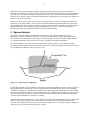
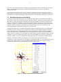


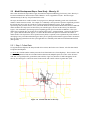
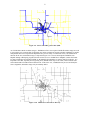
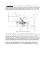


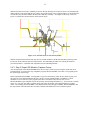


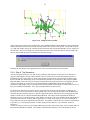

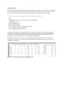
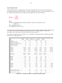

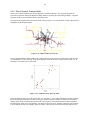
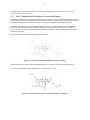
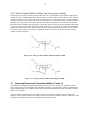


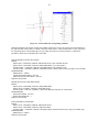
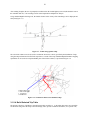


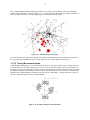


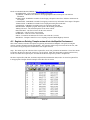
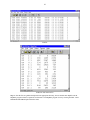
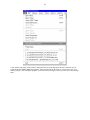
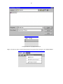
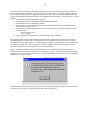
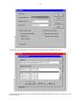
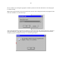
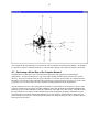
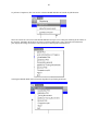


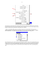


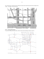
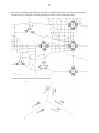
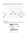


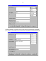
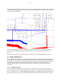


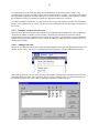
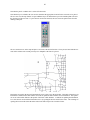
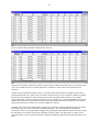
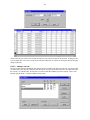
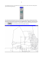


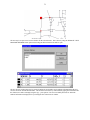

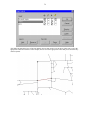
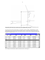


![ArcMap [v10.0- v.10.2] User manual](http://vs1.manualzilla.com/store/data/005724954_1-1f5d2da94c774511c91b8b97dbbbcd93-150x150.png)