Download 1 Kamel Simile Version User`s guide P. Martin, E

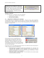
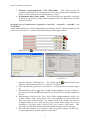
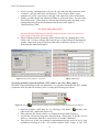
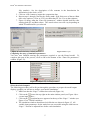
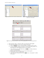
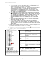
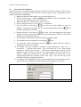
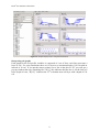
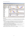
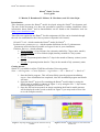
Kamel® user manual for Lab homework
Kamel® Simile Version
User’s guide
P. Martin, E. Braudeau, R. Mohtar, K. Cherkauer, and M. Abou Najm
Introduction
This document presents the Kamel® model developed using the Simile® development tool.
The aim of this document is to show the procedures required to conduct simulations. More
information about Simile® and its functionalities can be found on the Simulistics web site
(http://www.simulistics.com).
Three files are required to use Kamel® for this assignment (all files can be obtained through
the web site established for this class at pasture.ecn.purdue.edu/~kamel):
1.KamelV71.sml - which contains the Kamel® model for Simile®;
2.pedostructure parameters.cvs - which contains definitions for the 15 pedostructure
parameters used to define all possible soil types for use in your simulations;
3.Indiana_Rain.cvs - which contains:
• 2-Year Indiana: 2-Year 24-hour (low) intensity rainfall for 7 days (units: mm/hr).
• 25-Year Indiana: 25-Year 24-hour (high) intensity rainfall for 7 days (units:
mm/hr).
• ET Jan: Evapotranspiration data for 7 days in the month of January (winter) (units:
mm/hr).
• ET July: Evapotranspiration data for 7 days in the month of July (summer) (units:
mm/hr).
Getting started
Simile 4.7 is available in all the ITAP labs at Purdue University under:
Start -> All Programs -> Course Software -> agriculture -> FS -> Simile 4.7 -> Simile 4.7.
1. Start the Simile program. This will most likely open the program installation
screen. Once installation has completed, close the installation program and Simile
will start.
2. Open the Simile® project file containing the Kamel® model either by using the
Simile start-up window as shown on Figure 1, or by using the File -> Open menu,
and selecting the file kamelV71.sml.
3. Once the file has been opened, an image containing the Kamel® model structure
will be displayed on the screen as shown in Figure 2 (you may need to Zoom Out
to see the complete model).
Figure 1: Opening Simile® project file from the start-up
window
1
Figure 2: Kamel® model structure as seen within the
Simile tool.
Kamel® user manual for Lab homework
During the process of loading the Kamel model,
initializing the model parameters or running the
model you may receive the error message shown
to the right. This just warns that you are running
a trial version of the Simile tool and will not
impact you simulation. Click OK to clear the
message and proceed.
Running a simulation
The following steps are required for each new simulation.:
1. Setup the base conditions for the simulation;
2. Select the desired outputs;
3. Start the model simulation.
(1)
Setup the base conditions for the simulation
To setup Kamel for a new simulation, use the Model -> Run menu. After a short compilation,
the first window (Figure 3) called “Enter file parameters” will open. Within this window you
will identify the required parameter values by either entering them into the available boxes or
linking to existing data files.
Figure 3: Main Screen Input parameters window: top (left), after scrolling down (right).
Some users may receive an application error
message (Figure 4) at this time. Ignore this or
similar messages by clicking OK on every bow
that appears. This error appears to occur only
when multiple people try to start Simile and Kamel
at the same time and has not caused problems with
any of the following steps..
Figure 4: Application Error Message.
For the class exercise, the following parameters must be set within the “Enter file parameters”
window using the procedures detailed below:
1. Soil pedostructure properties for the four soil horizons: A1 <caractA1>, A2
<caractA2>, B1 <caractB1>, and B2 <caractB2>. These parameters define the
simulation characteristics of each of the four near surface soil horizons. All four
fields must be defined to run a simulation.
2. Soil horizon depths: <HorizonLimits>. This field defines the maximum depths
of each of the four soil horizons.
2
Kamel® user manual for Lab homework
3. Potential evapotranspiration: ETP <ETP_mmh>. This field provides the
estimates of potential evapo-transpiration rates for the duration of the simulation in
mm/h. If not set Kamel uses a default value of 1 mm/h.
4. Precipitation: Rain <Rain_mmh>. This field defines rain intensities, expressed
in mm/h, for the duration of the model simulation. If not set Kamel uses a default
value of 10 mm/h.
Specifying the soil pedostructure properties (<caractA1>, <caractA2>, <caractB1>, and
<caractB2>)
Kamel model parameters will be automatically generated by Simile® when the parameter file
pedostructure parameters.cvs has been loaded using the following procedure:
Figure 5: Use the
to fill each soil horizon with data from the soil parameter file..
Figure 6: Data input for first horizon, A1 <caractA1>
Figure 7: Select data from <pedostructure
parameters.cvs>
1. Open the window “Table data for …” by clicking on the
button located to the
right of each soil horizon field (e.g. <caractA1> in Figure 5).
2. Select the data file pedostructure parameters.cvs using the Browse button (Figure
6).
3. Drag and drop to move < > from <Table column headings> to <Use as indices>,
this selects the first column in the input file as the indices for all other columns in
the file.
4. Drag and drop <Selected_Soil_Type> from <Table column headings> to the <Use
as data column> field. You can use any of the available soil types (Silt Loam,
Silty Clay Loam, Loam (COLE=1.38), Loam (COLE=2.25), Sandy Clay Loam or
Averaged Value) as your <Selected_Soil_Type> based on the study case you are
working on. In Figure 8 the <Selected_Soil_Type> used is <Silt Loam>. This
procedure will fill in the Kamel model parameters using the selected soil type.
5. Once you have filled in <Use as indices> and <Use as data column>, click on OK
to import parameters from the input file into Kamel®.
3
Kamel® user manual for Lab homework
6. If you are using a homogeneous soil you can copy and paste the parameters from
<caractA1> into the other three soil horizons. If you want to define a more
complex soil profile, repeat steps 1 through 5 for each of the other soil horizons.
7. Finally, you must define the maximum depths or <HorizonLimits> for each of the
four soil horizons. This is done by entering the following values by hand (or by
cutting and pasting from this document) into the box to the right of
<HorizonLimits> field:
#1: 20 #2: 50 #3: 80 #4: 120
Be aware that the field must be entered exactly as shown or an error may occur
when trying to run the model simulation.
8. Figure 9 shows what the parameter fields will look like for a homogenous <Silt
Loam> soil. If you are using a different soil type, or have defined a inhomogeous
soil the values in the four soil horizon fields may be different, but the #1, #2, #, …
field identifies should still appear.
Figure 8: Specify data input for <caractA1>
Figure 9:Data input
Specifying potential evapotranspiration (<ETP_mmh>) and rain (<Rain_mmh>)
Potential evaporatranspiration and rain parameters are generated automatically after loading
parameters from the data file Indiana_Rain.cvs using the following procedures:
Figure 10: Use the
button to fill the potential evapotranspiration field with data from the data file.
1. Open the window <table data for> by clicking on the button
located to the
right of the ETP_mmh field (Figure 10).
2. Select the data file Indiana_Rain.cvs using the browse button (Figure 6).
3. As with the soil horizon properties, drag and drop <Time(min)> to fill the <Use as
indices> column (this data file is a time series of weather conditions).
4. Then select one of the two potential evapotranspiration time series to use in your
simulations and drag it to the <Use as data column> field. Figure 11 uses <ET
4
Kamel® user manual for Lab homework
July (mm/hr)>. See the description of file contents in the Introduction for
information on the choice of ET.
5. Click on <OK> button to import the evaporation data.
6. Repeat steps 1 through 5 but for the <Rain_mmh> field. Select one of the two Rain
time series options (2-Year or 25-Year) rather than ET for <Use as data column>.
7. Figure 12 shows what the “Enter file parameters” window should look like after
entering both ET and Rain values. The actual values seen will vary depending on
which ET and Rain files you selected.
Figure 11: Select data from < indiana_Rain.cvs >
Figure 12:Data input
Completing the entry of simulation parameters
You have now finished entering the parameters required to run the Kamel model. To
complete this part of the process, click on OK at the bottom of the “Enter file parameters”
window (Figure 13).
Figure 13:Complete entry of model parametes.
Select the desired outputs
The following procedures will walk you through the procedure to prepare the model output
displays (graphs) you will use to analyze your model simulations:
1. Make sure that the “Page 1” tab has been selected (Figure 14).
2. Click on the
icon to the top right on the main window panel (see Figure 14) to
<create input sliders> .
3. Click on the
icon that has now appeared at the top of the “Page 1” window (see
Figure 15) to <add all variables>.
4. The simulation window should now look like the one shown in figure 15. All
variable input parameters for the model are now accessible using the slide bars on
“Page 1” and can be adjusted here before each simulation.
5
Kamel® user manual for Lab homework
Figure 14: Blank execution window for Kamel model
Figure 15: Execution window after sliders for all
variables have been added.
Figure 16: “Page 2” panel divided into 6 panes, four for graphing data, two for controlling parameters.
5. Now select the “Page 2” tab, this is where you will create output graphs.
6. The following proceedure will create six graphs on this page.
a. Click on the
icon twice to split the window vertically into three panels.
b. You can resize these windows vertically, by moving the mouse pointer over
the dividing lines and dragging the line to a new location.
c. Click within the upper panel and click on the
icon to further divide the
window panel horizontally.
d. Repeat c, but click each of the other two lower window panels
e. You should now have six blank panels.
icon to “create plotter” or add a
f. Click in the upper left panel then click the
blank graph.
6
Kamel® user manual for Lab homework
g. Use the scroll bar under the “Run control” panel to scroll through the list of
model parameters until you reach the group heading
“RSV_WaterProfileOutput” (Figure 17a). These are model output parameters
defined from the soil surface to the depth of the forth soil horizon (see
<HorizonLimits>) at a default interval of 10 cm. Therefore layer 1 is at a
depth of 10cm, layer 2 and 20cm, through the 12th layer at a depth of 120cm.
The variable types are defined in Table 1.
h. Lets set this graph to plot gravimetric water content for all layers. Select the
icon at the top of the plot you just created to “add a variable”, then click on
“W” under the group heading “RSV_WaterProfileOutput” (Figure 17). The
plot should now have a blue line followed by the text “W, run 1”. This
indicates that W for all layers will be displaed as blue lines on the current
graph.
i. Repeat steps f-h to create three more plots in the top panels using variables
Wma, Wmi and Vpfiss from Table 1.
j. For the bottom two panels, repeat steps f-h, but scroll down the model
parameter list futher until you find the group “ETP and RAIN” (Figure 17b)
and setup one plot for potential evaporation (ETP_mmh) and the other for Rain
(RAIN_mmh).
7. Graphs can be cleared and restarted by selecting the
icon for each graph or for
all graphs by selecting the one at the top of the windowl.
icon, then selecting the
8. Variables can be removed from a graph by selecting the
variable to remove from the list that appears.
a.
b.
Figure 17: Listing of model output
variables as display in the execution
window. Must scroll down list to see (a)
soil profile variables and (b) ET and
rainfall variables.
W
Gravimetric water content of the soil at
time t (mm/mm)
Wma
Macropore water content at time t
(mm/mm)
Wmi
Micropore water content at time t
(mm/mm)
Vpfiss
Volume of soil cracks at time t (m3/kg)
ETP_mmh
Potential evapotranspiration at each time
t (mm)
Rain_mmh
Rainfall at each time t (mm)
Table 1: Definitions of useful model output parameters
7
Kamel® user manual for Lab homework
(3)
Start the model simulation
Now that you have set-up the model parameters and laid out slider controls to allow you to
change parameters and displays that will show you the results of your simulations, you are
ready to start model simulations.
1. Make sure that the “Run control” tab is selected (Figure 18).
2. Set the “Execute time:” field for 10080 units (minutes for these simulations. This
will cause the simulation to run for a full week.
3. Make sure that the “Current time:” field is set to 0.
4. Set the “Display interval:” to 10 units (i.e. 10 minutes).
5. Clear all plots by selecting the
icon at the top of the window to clear all
displays. Note that each graph can be cleared independently using the
icon
located within that plot window.
6. Run the model by selecting the
icon, lines will start appearing in the graph
windows and the current time field will start incrementing. Figure 19 shows the
display for a completed model run.
7. The simulation can be paused by selecting the run button again.
8. The simulation can be stopped by selecting the
icon.
icon again while the model is
9. To repeat the current simulation select the
stopped, then repeat steps 5 and 6.
10. To change soil type, rainfall or potential evapotranspiration, select File ->
Parameters … from the main menu. This will return you to the “Enter model
parameters” window from section 1. Follow those instructions to change the file
parameters (note you do not need to reset all parameters, just those you want to
change). When you click on OK to close that window you will return to your
model output parameter windows as they were setup. You can now run a new
simulation using the changed parameters.
11. To compare two simulations, do not clear the graphs between simulations (step 5).
Lines for the new simulations will be added to your graphs in a new color.
Figure 18: Run control tab
8
Kamel® user manual for Lab homework
Figure 19: Sample display from a completed simulation
Interpreting the graphs
Each graph for the soil profile variables is composed of a set of lines, each line represents a
layer of soil. For your simulations there are 12 layers to a maximum depth of 120 cm with an
interval of 10 cm. If you put the mouse pointer over a line in the plot of “W” you will get a
pop-up window that says something like “W[1]” this indicates that the line is for the first soil
layer (depth 10 cm), “W[12]” indicates the 12th or bottom most soil layer with a depth of 120
cm.
9
Kamel® user manual for Lab homework
References
The soil parameters used in this notice were estimated by the authors using the pedostructure
concept developed by Braudeau et al. 2004 and Braudeau and Mohtar 2004, 2005, 2006
presented in :
Braudeau, E., J.P. Frangi, and R.H. Mothar. 2004. Characterizing nonrigid dual porosity
structured soil medium using its Shrinkage Curve. Soil Sci. Soc. Am. J. 68:359-370.
Braudeau, E., R.H. Mohtar, and N. Chahinian. 2004. Estimating soil shrinkage parameters. In:
Y. Pachepsky and W. Rawls (eds) Development of Pedotransfer Functions in Soil
Hydrology, pp. 225-240. Elsevier, Amsterdam.
Braudeau, E., and R.H. Mohtar. 2004. Water potential in nonrigid unsaturated soil-water
medium. Water Resources Research 40(5): W05108.
Braudeau E., Sene M., and R. H.Mohtar. 2005a. Hydrostructural characteristics of two
African tropical soils. Eur. J. Soil Sci. 56, 375–388.
Braudeau E. and R. H. Mohtar. 2006. Modelling the swelling curve for packed soil aggregates
using the pedostructure concept. Soil Sci. Soc. Am. J. 70:594-502.
10