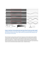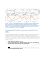
1
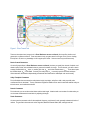
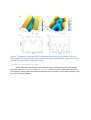
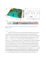
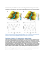
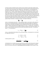
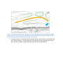
River Synth
©
V1.1
User manual for building synthetic digital
rivers
Rocko Brown, PhD
10/8/2015
Please cite as: Brown, R.A. 2015. RiverSynth V1.1 Users Manual. Revision to 2014 manual.
Copyright Rocko Anthony Brown 2012.
River Synth© V1.1
User manual for building synthetic digital rivers
Updates and new features:
•
•
•
There are instructions and an example on how to create a synthetic channel
within an existing terrain for river restoration design.
There is now a minimum channel width cell you can use to limit width oscillations
from overlapping.
There is a channel boundary tab that allows you to easily export the centerline
and channel width points to create bounding polygons for surface creation or
2D modeling.
Acknowledgments:
My advisor and collaborator Dr. Greg Pasternack (www.pasternack.ucdavis.edu) provided critical moral support and
input in writing the manuscript during my PhD.
My collaborator Wes Wallendar provided critical discussions and input on the coordinate transformation and the use
of notation in the manuscript.
My colleague Jason White at ESA has significantly improved the model and has become an expert at using it within
AutoCad for river restoration design. He is a good resource if you have questions – [email protected]
Partial indirect funding was provided by a Henry A. Jastro Graduate Research Award, a research grant from the U. S.
Army Corps of Engineers (award # W912HZ-11-2-0038), and a Hydrologic Sciences Graduate Group Fellowship.
Contents
Introduction ............................................................................................................................................................ 5
The Origins of River Synth ...................................................................................................................................... 5
How to use it .......................................................................................................................................................... 5
Units ...................................................................................................................................................................... 7
Versions ................................................................................................................................................................. 7
Free Programs for Viewing and Analysis ................................................................................................................. 7
Using the GCS to create idealized topographies ...................................................................................................... 8
Designing channels with form-process assemblages ............................................................................................. 11
Creating a nested channel for river channel creation in the “real world” .................................................................. 14
Side channel design example................................................................................................................................ 16
Caveats ................................................................................................................................................................ 21
References ........................................................................................................................................................... 21
Figures
Figure 1. River Tweak Tab ..................................................................................................................................... 6
Figure 2. Topographic surface and GCS’s for prototypical lowland (A,B) and upland (C,D) rivers illustrating the how
varying GCS’s can create different channel configurations. Contour lines are at intervals of 2m and labels are omitted
for clarity. ............................................................................................................................................................... 9
Figure 3. Topography (A) , GCS (B) , and tweak parameters using the 4h synth model (C) for a meandering river .10
Figure 4.Surface topography and GCS illustrating the use of the GCS between channel and valley elements in
creating indirect topographic features. Refer to text for descriptions....................................................................... 11
Figure 5. Synthetic test beds and dimensionless bed and width profiles for the synthetic test beds analyzed in this
study. All scenarios have the same slope of 0.002. S1 (A,B) has no bed or width undulations, S2 (B,C) has only
width undulations, S3 (D,E) has only bed undulations, S4 (F,G) has bed and width undulations that covary in phase
and S5 (H,I) has bed and width undulations that also covary but are out of phase. ................................................. 13
Figure 6. Top: Plots of relative width (black dashed) and relative bed elevation (solid black), and water surface
elevations at 5 (light blue) and 125 (dark blue) m3/s for scenarios 2 through 5. Bottom: Plots of shear stress at 5
(orange) and 125 (red) m3/s for scenarios 2 through 5. Note that scenario 1 is not shown because there is no
topographic or hydraulic, variability. Note that a reversal in peak shear stress only occurs for S4 (E,F)................... 14
Figure 7. Basic ARCGIS steps for nesting a SRV model into a real world terrain. Based on subsequent modeling of
the final composite terrain, each river reach can be adjusted to optimize physical habitat and the occurrence of
hydrodynamic and geomorphic processes. ............................................................................................................ 15
Figure 8. Examples of channel structure manipulation for the south channel. Profiles start at the yellow star on the
left and go upstream in distance to the right yellow star. The channel topography for each scenario was adjusted by
altering the phase of the GCS between bed elevation and width, showing how riffle and pool widths can be adjusted.
............................................................................................................................................................................ 16
Figure 9. Map of study area showing existing contours in black, manually graded contours in green, and the side
channel SRV alignment in blue. The blue arrow denotes the flow direction of the main river channel. ..................... 17
Figure 10. Alignment (dark blue line) and point cloud (red dots) showing the synthetic channel domain where the
centerline was oversampled relative to the synthetic channel domain. The blue arrow denotes the flow direction of
the main river channel. .......................................................................................................................................... 18
Figure 11. Alignment (dark blue line) and point cloud (orange dots) showing the synthetic channel domain where the
synthetic channel domain was modified to match the alignment sampling. The blue arrow denotes the flow direction
of the main river channel. ...................................................................................................................................... 19
Figure 12. Two surface scenarios (C,F) for the design of the side channel along with planform (A,D) and covariance
plots (B,E) as discussed in the text. ....................................................................................................................... 20
Introduction
Welcome to the first version of River Synth ©, an excel model for creating XYZ points for synthetic river
valley topography. The theoretical basis for River Synth© is described in the publication, “Synthetic river valleys:
creating prescribed topography for form-process inquiry and river rehabilitation design”, published in the journal,
Geomorphology (Brown et al, 2014). For a longer version that is more comprehensive see my PhD dissertation
(Brown, 2014). Further, I have several publications in preparation that show how you can use this tool for river
restoration design and form-process inquiry.
This is intended to be a living document with the goal of explaining how to use an Excel version of the model
to create synthetic river valley topography. If you have questions or ideas to make this better contact me!
The Origins of River Synth
When I first began my PhD I initially wanted to study waterfalls. At the time I was living in San Francisco
and thought that if I could get a project near my home it would allow me to go to UC Davis while not having to move
there. There are a lot of small waterfalls in the Bay Area I thought I would study but that didn’t pan out for logistic
reasons. My next option was to continue working on gravel bed rivers, but with so much research already done on
these types of rivers I had trouble seeing where I could contribute. One day at lunch with my graduate advisor, Greg
Pasternack, he suggested I try generating artificial rivers. At first, a swell of differential equation for water and
sediment mass, momentum, and energy conservation smacked me in the head and made me feel there is no way I
can create rivers using the full equations of motion – what I felt was the best way at the time. Well, I could, but I felt
I’d be embarking on a decade long PhD. What I ended up doing was relying on my experience designing and
building rivers in the real world from my experience as a consultant. In engineering applications there is a heavy
reliance on the channel cross section and profile to convey both existing conditions and design scenarios. CAD
programs typically require the user to specify an alignment (where the river is in horizontal space), a typical cross
section and a profile and these are combined in surface modeling to create design topographies. A detriment to this
approach is that it’s not possible to use adjustable control functions for these elements that change with distance.
Further, these programs are expensive and not freely available. I’ve tried to address some of these issues with this
program, but it is not meant to compete either!
How to use it
Using the model is really simple. Overall, you set reach averaged variables and then use parameters of for each
geometric element listed up top on the River Tweak tab. You can then take the XYZ coordinates from the tab XYZ
and use them however you want.
Before getting into further details I’ll provide an overview of the tabs.
River Tweak – This tab allows you to set variables and tweak parameters. Blue cells can be modified by the user,
green cells are calculated based on inputs, and orange cells are constant. This is the main tab the user interfaces
with and will be discussed in more detail later in this document.
Figure 1. River Tweak Tab
There are three plots here (orange circle in Error! Reference source not found.) for the profile, planform, and
geomorphic covariance structure. These are meant to help you get a sense for the type of river you are creating.
Excel plots in 3D, but to my knowledge not for irregular point clouds. I’d love to hear if anyone knows a way!
Reach Channel Parameters
On the left (purple ellipse in Error! Reference source not found.) is where you specify the channel, floodplain, and
domain inputs in blue, with calculated values in green and constants in orange. For the channel, you enter a reach∗
average bankfull width, , slope, , median grain size, , and critical shields stress, . From these inputs
the bankfull depth, is calculated. Currently, the valley slope, , is currently equal to the reach bed slope.
Other measures calculated to independently parameterize the model are the width-depth ratio and sinuosity.
Valley Floodplain Parameters
For the floodplain the user enters the valley bottom height, top height, valley floor width, valley top width and a
confinement ratio is calculated. The top and bottom heights and widths can be used to make wide and flat valleys or
tall and narrow, and combinations thereof.
Domain Parameters
For the domain you can set the vertical datum and the total length. Note that with a set number of model nodes you
can increase and decrease the resolution by adjusting the length.
Tweak Parameters
On the top are the parameter cells for the amplitude, frequency, and phase for each geometric element with units of
radians. For geometric elements such as the Alignment, Bankfull Channel Width, Bed, and Right and Left
Floodplains that have four columns the cells alternate across from cosine to sine twice (e.g. cosine, sine, cosine,
sine) as in Equation 5 in Brown et al. (2014). These cells essentially describe the sub-reach variability of the
synthetic channel. With four different superimposed waveforms the synthetic channels can be quite complex.
Some of the parameters have “practical limits” before the waveforms cross over each other. This can especially
happen with high alignment and width frequency combinations.
Channel Model - This tab is where the channel model is formulated. As discussed later, this is where you can
paste in a real world centerline.
Floodplain Model - This tab is where the floodplain model is built. You can also paste in real world coordinates
here in place of modeled floodplain variability.
XYZ – This is the XYZ output of the synthetic river valley. You can take these points and use a separate program to
visualize or model the surface you create. By producing only an XYZ it allows the user to drive subsequent steps
with complete freedom using whatever software platform they desire.
Hidden Tabs – These tabs are hidden from the user but do all of the heavy lifting. If you want a version with
those open just ask. All I ask is that folks who modify the spreadsheet share it with me so I can host them all here.
•
•
•
XS Model – This tab is where the cross section model is built, creating asymmetric cross sections based on
the channel curvature.
Coord Trans – This tab transforms the river from s,n to x,y coordinates.
Covariance – This tab calculates standardized residuals for each spatial series and the covariance between
certain geometric elements.
Units
The model is built to be in metric. Each waveform parameter (cells in the red ellipse) has units of radians.
Versions
There are two main versions of RiverSynth available:
•
•
RiverSynth V1.0 - SRV4H – this is a model that has pairs of alternating sines and cosines for the geometric
elements.
RiverSynth V1.1 - RealSimple – this is a single sinusoid model setup for importing centerlines for real world
applications
Free Programs for Viewing and Analysis
Some free terrain programs for viewing and further analysis:
•
•
VTBuilder (http://vterrain.org/Doc/VTBuilder/overview.html)
Landserf (http://www.soi.city.ac.uk/~jwo/landserf/download)
Using the GCS to create idealized topographies
For RiverSynth dependent parameterization of the geometric model is contextualized by the spatial
covariance of specific geometric elements, which is termed the geomorphic covariance structure (GCS). A GCS is a
spatial covariance relationship between two or more geometric attributes in a river valley. For example, the serial
covariance, , between pairs and can be calculated from detrended and standardized series residuals,
and by the product, . The basis for the use of a GCS in dependent parameterization is that alluvial river
systems in dynamic equilibrium can have ideal relationships between the covariance of specific geometric variables,
such as ZT and WBF or ZT and CS that can aid in dependent parameterization (Brown and Pasternack, 2012).
Interpretation of a GCS is based on the sign of the covariances. For example consider three basic cases: (i) if
> 0 and > 0 then > 0, (ii) if < 0 and < 0 then > 0, and (iii) if or are < 0 then
< 0. Thus, when > 0 the local geometric elements covary and when otherwise do not. By thinking
through how and where variables that control geomorphic process need to covary it is possible to design a GCS to
operationalize a geomorphic process concept via tailored nonuniform, stage-varying channel forms to yield functional
form–process dynamics.
Straight rivers
Straight rivers are really simple to build. Simply set all of the tweak parameters to 0 (e.g. no osciallations). That’s it!
Bed and width undulations
As described in my dissertation and in an AGU presentation (Brown and Pasternack, 2012) rivers have distinct
GSC’s for different landscape settings. For the examples in Figure 2, a single waveform (Eq. 5;
= 1; , ! , " = 0) was used for #$ and to illustrate the utility of GCS manipulation in creating straight
channels with varying topographic surfaces (Figure 2). For Figure 2, %$ , & ≥ 0, which has the effect of
creating topographic high points in areas that are locally wide and topographic low points in areas that are locally
wide, consistent with geomorphic theory (Figure 2A,B). Using the sign of %$( ) as an index for riffle and pool
locations, where %$( ) > 0 are riffles and %$( ) < 0 are pools, station 100 would be classified as the center of
a riffle where stations 0 and 325 would be pool centers. In contrast, S2 has %$ , & ≤ 0, which has the effect
of creating topographic high points in areas that are locally narrow, which is also consistent with the
conceptualizations envisioned in the first step of the modeling process (Figure 2C,D). Using relative bed elevation as
to discriminate between riffles and pools, stations 50 and 125 would be the center of a riffle or step, while stations 18
and 88 would be pool centers. Together with independent parameterization for the reach-average variables the GCS
of geometric elements that have simple control functions can create the topography of idealized end-member
landforms associated with mountain and lowland settings.
Figure 2. Topographic surface and GCS’s for prototypical lowland (A,B) and upland (C,D) rivers
illustrating the how varying GCS’s can create different channel configurations. Contour lines are at
intervals of 2m and labels are omitted for clarity.
Equilibrium meandering rivers
Alluvial lowland pool–riffle channels in quasi-equilibrium may be characterized as having quasi-oscillatory
GCS patterns where %$ , & ≥ 0 and %$ , +, ≤ 0. To create a pool at each outside bend and a riffle at
each bend apex, thalweg elevation and channel curvature were set out of phase by π/2 and centerline frequency was
set to 1/2 of the thalweg frequency.
(C)
Figure 3. Topography (A) , GCS (B) , and tweak parameters using the 4h synth model (C) for a
meandering river .
Valley Configurations
Until this point, the focus was on GCS’s for channel elements without considering the relative structure of
the channel planform, - , valley floodplain, and how floodplain features can be indirectly created through
interpolation. To illustrate this let’s evaluate how parameter manipulation can alter the GCS and model topography
when #./ > 0 and focus on the interaction of - and the left and right planform coordinates of ./ , that is for
both 0 , 1./ and 0 , 2./ . The examples in Figure 4 were parameterized so that 0 , 1./ 0
and 0 , 2./ 0, meaning that they covary along 0 . The opposite signs of 3(0 ) in Eq. (9-10) require that a
phase shift of 4 be applied to one of the valley floor coordinates and in this case, the left valley floor coordinate,
1./ (0 ), so that both sides follow (0 ). For such a GCS (Figure 4C) the topography has features indirectly
created through interpolation as stations 500, 1000, and 1,500 that visually appear to represent gradual hillslopes
that fall down to the channel edge (Figure 4A). When the phase shift for 1./(0 ) is removed and added to (0 )
however, the GCS, 0 , 1./ is * 0and has an oscillating structure that is symmetrical to 0 , 2./ (Figure
4D). The topography then has features akin to an alluvial fan (Chant et. al., 1999) at stations 0, 1000, and 2000
(Figure 4B). Regardless of the harmonic organization between channel meandering and valley floodplain, when
#./ 0a broad, flat floodplain is created, but no indirect valley features are created via interpolation. This
illustrates that while planform GCS’s can be useful in contextualizing relationships between geometric elements,
consideration of vertical relationships is also important in creating 3D topography within the channel and floodplain.
Figure 4.Surface topography and GCS illustrating the use of the GCS between channel and valley
elements in creating indirect topographic features. Refer to text for descriptions.
Designing channels with form-process assemblages
In this section I’ll briefly describe how we can create topographic surfaces with form-process assemblages. What I
mean by form-process assemblages is that certain landforms create certain hydraulic and geomorphic processes.
For example, if we think of a river valley leaving the headwaters of a mountain range and opening up onto the valley
floor we can appreciate that the change in topography from being confined and steep to unconfined and flatter
reduces water speeds and can lead to deposition of whatever the water is carrying. Another example is a waterfall
step where flowing water plunges over and creates a scour pool. Both of these examples, while at different spatial
scales have distinct processes of water flow (and thus sediment transport) associated with the topographic form.
While this concept is relatively new, we have dialed in one specific process associated with riffle-pool maintenance.
This is discussed in chapter 4 of my dissertation (Brown, 2014) as well as in a publication currently under review
(Brown et al., Submitted). For the remainder of this section I will summarize the key ideas.
For riffle-pool couplets a tremendous amount of research into their maintenance and formation suggests an ideal
GCS, where at some channel forming flow the topographic high points have wider flow widths than topographic low
points (Keller, 1978; Carling and Wood, 1994; Thompson et al., 1999; Wheaton et al., 2004; MacWilliams et al.,
2006; Harrison and Keller, 2007; Caamano et al., 2010; Sawyer et al., 2010; Thompson, 2010; White et al., 2010;
Rhoads et al., 2011). Therefore, the GCS needed for RP unit maintenance requires positively covarying bed and
bankfull width oscillations. One the basis of 1D analysis there is quantitative guidance on the relative variations of
width and depth needed for flow convergence that can be used to further quantify the GCS (Carling and Wood, 1994;
Caamano et al., 2009). Using a 1D hydraulic model Carling and Wood (1994) found that they need to be 50% wider
than pools or pools need to be rougher than riffles for a reversal in mean velocity. Caamano et al (2009) developed a
state space that suggests that both width and depth variations are controls on whether a flow reversal occurs.
Specifically, for uniform roughness and assuming equal head losses they show that width variations need to be
greater than depth variations for a convergence or reversal. The Caamano relationship is:
56
57
=1+
96
96:;
(1)
where ℎ= is the flow depth over the riffle, ℎ=>, is the residual pool depth, = is the width of the riffle and ? is the
width of the pool at the bankfull discharge. For simple case where bed and width undulations are modeled by a
sinusoid and are in phase with the same frequency we can mathematically relate the SRV model to the Caamano
@@@@@
relationship. Based on the fundamental SRV equations (Brown et al., 2014) , ℎ= is equal to . The residual pool
depth, ℎ=>, , can be determined as the vertical difference between the maximum and minimum bed undulations (e.g.
the riffle crest and pool trough, respectively) and accounting for the fact that the bed is sloped. The residual pool
depth, ℎ=>, , can be determined as:
@@@@@@@
5DE
@@@@@
ℎ=>, = 2
̅
B − 4
(2)
FG
where B is the amplitude of bed undulations and !B is the angular frequency. Assuming there are no phase shifts
the relative widths are given as:
@@@@@@
@@@@@@
= = I + (3)
@@@@@@@@
@@@@@@
? = −
I + (4)
Combining equations 1-4 yields:
@@@@@@@
@@@@@@@
5DE JK L5
DE
@@@@@@@
M5
J
L5
DE K @@@@@@@
DE
=1+
@@@@@@
NDE
@@@@@@@@
QDE
@@@@@@
ON
S̅
DE JG MP
(5)
RG
and illustrates how one can adjust a terrain with the state space of the Caamano criteria using the reach-averaged
input values and B , I and !B for when the frequency and phase of the waveform are equal for #$ and .
Below are five surfaces, where the forth one (Error! Reference source not found.G,H) follows equation 5 above.
Figure 5. Synthetic test beds and dimensionless bed and width profiles for the synthetic test beds
analyzed in this study. All scenarios have the same slope of 0.002. S1 (A,B) has no bed or width
undulations, S2 (B,C) has only width undulations, S3 (D,E) has only bed undulations, S4 (F,G) has
bed and width undulations that covary in phase and S5 (H,I) has bed and width undulations that
also covary but are out of phase.
While the surfaces may seem trivial they highlight how the topography can be easily adjusted and how different
covariance patterns create different channels. To show why these matter, we have to appreciate that riffle-pool
maintenance is founded on covarying bed and width oscillations that create reversals in velocity or shear stress
between low and high flows. To show this, Figure 6 shows plots of relative bed elevation and bankfull width and
water surface elevation and shear stress for a base and bankfull flow discharge. Note that the only surface that has a
reversal is the one with both bed and width undulations in phase, consistent with theory.
Figure 6. Top: Plots of relative width (black dashed) and relative bed elevation (solid black), and
water surface elevations at 5 (light blue) and 125 (dark blue) m3/s for scenarios 2 through 5.
Bottom: Plots of shear stress at 5 (orange) and 125 (red) m3/s for scenarios 2 through 5. Note that
scenario 1 is not shown because there is no topographic or hydraulic, variability. Note that a
reversal in peak shear stress only occurs for S4 (E,F).
Creating a nested channel for river channel creation in the “real
world”
Overview
The real world examples using the “RiverSynth V1.1-RealSimple” excel books. Before we get into details there are
some basics we needed to discuss. Since we are creating a new channel(s) we need to specify some basic
parameters and also require some essential data. We obviously need a DEM that we can nest/embed the synthetic
channel into. Also, as with any SRV, we need to determine the average bankfull width, an equilibrium slope, channel
typology for each segment, and the spacing of riffles and pools. Then, to embed your SRV into a terrain are several
steps as shown in Figure 4.
1. Specify a design corridor that the SRV will go into.
2. Convert your DEM to contours and clip everything out within your model domain. If you are working with
points then exclude or delete all existing data within your design corridor.
3. For each of the channels a centerline was drawn in ARCGIS and discretized at approximately 1m (Figure 7).
4. Next, these centerlines were used as inputs in the RiverSynth program to create topographic models for
each channel. The order of point’s matters, so look at what your direction is relative to how the model is
setup.
5. Once the centerlines were added, geomorphic covariance structures were used to parameterize the joint
variability of the bed and bankfull width variability.
3. Draw centerlines and establish node
spacing. Note that areas between
centerlines were manually edited.
4. Import point cloud into surrounding
terrain. Note that areas not within the
point domain were manually edited.
5. Generate terrain model. Contours are 1
foot intervals
Figure 7. Basic ARCGIS steps for nesting a SRV model into a real world terrain. Based on
subsequent modeling of the final composite terrain, each river reach can be adjusted to optimize
physical habitat and the occurrence of hydrodynamic and geomorphic processes.
While Figure 7 shows the basic steps in nesting a synthetic river valley in a terrain, it doesn’t highlight the ease at
which the surface can be manipulated. To show this, Figure 8 is a plot of two scenarios and their geomorphic
covariance structures (for bed elevation and width and bed elevation and curvature). For these examples, the phase
of bankfull width was shifted from scenario 1 to scenario 2 shifted, resulting in scenario 1 having wide riffles and
narrow pools, while scenario 2 had narrow riffles and wide pools.
Figure 8. Examples of channel structure manipulation for the south channel. Profiles start at the
yellow star on the left and go upstream in distance to the right yellow star. The channel topography
for each scenario was adjusted by altering the phase of the GCS between bed elevation and width,
showing how riffle and pool widths can be adjusted.
Side channel design example
This example shows you how to create an SRV for a side channel design and is more detailed then the above
example. For this example I used ARCGIS©, although other platforms are possible for terrain editing and
visualization.
1. Convert existing topography to contours. Give some thought into the needed contour intervals. This will
affect how much time is needed to clip and modify the existing terrain for the SRV.
2. Modify the contour data set by clipping out the appropriate areas for the SRV, creating a clipped corridor. At
this point you may also want to manually grade transition or non SRV areas.
3. Draw a centerline for the SRV through the clipped corridor and measure the length. In the current
RiverSynth© program (V1.1) there are 758 nodes, so you want to generate nodes along the centerline in
ARCGIS at a spacing equal to: length of centerline divided by number of nodes. In this example the
centerline is 619 feet long, so the node spacing is ~0.8 ft. Now you can create points along your centerline
spaced at 0.8 ft. I usually use ET Geowizards for this by first densifying the centerline at the appropriate
node spacing and then Once that is done, add fields for X and Y, and use the ‘calculate geometry’ function
in ARCGIS© to determine their coordinates.
Figure 9. Map of study area showing existing contours in black, manually graded contours in green,
and the side channel SRV alignment in blue. The blue arrow denotes the flow direction of the main
river channel.
4. Export the XY coordinates of the centerline and you can now open up the RiverSynth©v1.1 RealSimple
Excel program. Go to the channel model tab and paste in your coordinates into the green X and Y cells as
shown below.
5. Now the alignment is in the RiverSynth© excel model. To check, your channel should be plotted in the
planform plot on the river tweak tab. Now you can start to set the basic parameters of the channel model.
a. Set the average channel width. Note that you can control where expansions and contractions are
located using the bankfull width waveform parameters.
b. Set the bankfull depth. This could be determined using empirical or analytical equations, or by
setting the depth equal to some tie in elevation with the surrounding terrain. The current model
uses the Shields Criterion, based on specifying the Shields parameter, sediment grain size and
slope. If you want to over-ride this, just paste your value in the cell.
c. Set the average slope
d. Set the datum to match the bed profile to your real world tie in. I usually approximate this by
adjusting the datum until the bed profile plot.
6. Take note if for some reason more or less nodes were created in ARCGIS©. If there are more you can
simply crop the alignment at the upstream or downstream location. If there is less, you may want to redraw
the alignment. For example, in the below figure you can see the top part of the alignment (dark blue line)
has no points (red dots). In looking at the centerline tab the alignment was oversampled (810 nodes).
Figure 10. Alignment (dark blue line) and point cloud (red dots) showing the synthetic channel
domain where the centerline was oversampled relative to the synthetic channel domain. The blue
arrow denotes the flow direction of the main river channel.
Since the imported points (red dots) also overlap with the grading associated with a riffle at the downstream
tie in, it makes sense to crop the lower excess nodes. You can see below the points are now start at the
upper end of the alignment and don’t intersect the lower grading (green lines).
Figure 11. Alignment (dark blue line) and point cloud (orange dots) showing the synthetic channel
domain where the synthetic channel domain was modified to match the alignment sampling. The
blue arrow denotes the flow direction of the main river channel.
7. Changing the surface. The plot below shows two different synthetic channel planform and GCS plots along
with a TIN for each surface. The left scenario has an average width of 20 feet, while right scenario has a
width of 50 feet. In addition, the bankfull width waveforms were parametrized differently.
Figure 12. Two surface scenarios (C,F) for the design of the side channel along with planform (A,D)
and covariance plots (B,E) as discussed in the text.
In looking at the left scenario (e.g. Fig4C) note that the channel has cross stream asymmetry at the upstream bend
and then becomes broad and symmetric towards the middle of the straight section. Also, we can see the exit
doesn’t transition smoothly. To fix this we could simply adjust the point cloud in that area or, create contours and
manually smooth the transition. Or we can also adjust the shape of the channel by increasing the average width and
manipulating the width harmonics by creating a pinch at the curve, where the channel is constricted by tree islands,
and expansion below where the side channel corridor is wider. This is what was done for the right scenario, as
shown in Fig4F.
We make these types of changes by adjusting the waveform parameters of the bankfull width.
1. The left scenario uses the first sine and cosine term of the waveforms only. The amplitudes are 0.2 and 0.3
for the sine and cosine and both angular frequency values are set to 1, and the cosine term (second
waveform cell) phase shifted by “pi”. See the screenshot below.
2. The right scenario also only uses the first sine and cosine term of the waveforms. The amplitudes are 0.5
and 0.01 for the sine and cosine and both angular frequency values are set to 1, and the cosine term
(second waveform cell) phase shifted by “pi”. See the screenshot below. See the screenshot below.
Hopefully this example helps you get going. As always let me know if improvement can be made in explaining the
process.
Caveats
•
•
•
•
I am not a programmer!
The two tabs in the model that the user interfaces with are the “River Tweak” and “XYZ output” tabs. All of
the other tabs are locked and hidden. If you see improvements that can be made let me know and I can
provide an unlocked version.
The critical depth for sediment mobility is determined based on the Shields equations (see the original
manuscript for the full equations). This means that for certain combinations of grain size and slope that very
shallow depths are predicted. This can create very shallow channels. To over-ride this, just insert the
bankfull depth value instead of having it calculated from the Shields equation.
It is possible to create unnatural surfaces in River Synth for specific channel width and alignment parameter
settings where the waveforms overlap.
References
Brown, RA, Lin, T, Pasternack, GB. In review. The topographic design of river channels for form-process linkages
for river restoration.
Brown, R.A., Pasternack, G.B. and Wallender, W.W., 2014. Synthetic River Valleys: Creating Prescribed Topography
for Form-Process Inquiry and River Rehabilitation Design. Geomorphology 214.
Brown, R.A. 2014. The Analysis and Synthesis of River Topography using Geomorphic Covariance Structures. PhD
Dissertation. University of California, Davis.
Brown, R.A. 2012. Synthetic River Valleys. 30th Annual Salmonid Restoration Federation Conference.
Brown, R.A. and Pasternack, G. 2011. Synthetic River Valleys. EOS, Transactions of the American Geophysical
Union EP21B-0693