Download The Noise Lab

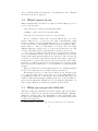
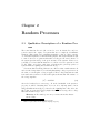
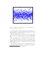
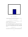
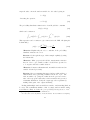
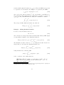
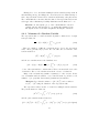
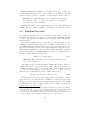
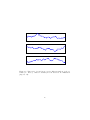
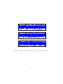
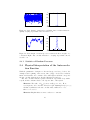
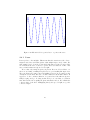
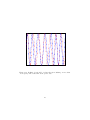
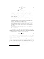
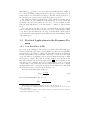
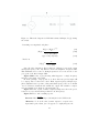
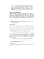
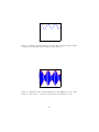
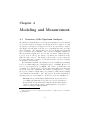
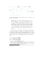
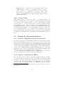
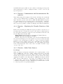
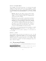
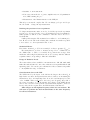
The Noise Lab
Chris Takacs
Chapter 1
Introduction
1.1
Goals of this lab
Our goal is to do a precision measurement of kb , Boltzmann’s constant. To
find Boltzmann’s constant, we measure voltage fluctuations known as Johnson
Noise over a resistor using a Spectrum Analyzer (SA). The SA is a complicated
piece of equipment and the measurements we want to perform will push their
limits. Thus, we need to understand how these instruments work at their most
basic level.
The first section is about understanding the properties of Johnson Noise as
well as other Random Processes. Dealing with random processes is very different
than deterministic systems. Developing tools to work with such systems is useful
in a wide variety of fields. We will quote the properties of Johnson Noise and
leave the physics of this phenomena to the references. The reason for this is
simple: there are already excellent derivations of this phenomena and I want
to focus myattention to developing tools to understand these derivations. The
tools are more similar to those in quantum and statistical mechanics than those
of classical mechanics.
The second section will be focused on creating a set of tools in the frequency
domain. We start this section off with a review of Fourier Transforms and their
properties. The emphasis is not on carrying out tedious calculations, but using
the properties of Fourier Transforms and graphical techniques to quickly find
the answers. This is to help build physical intuition when dealing with the
frequency domain.
The third section is about taking data with the SA . The goal of the previous
two sections was to develop the conceptual basis to understand the workings of
the SA amplifier. We start with developing a model based on the first two
sections, access the limitations and capabilities of each instrument and create a
testing regime.
The final section is a brief overview about extracting kb . Most of the fitting
is done with a simple Mathematica script provided with the lab. From the
1
data, you will determine the useful range of the instrument. Also, additional
directions for the lab are suggested.
1.2
What I expect of you
This is an ambitious lab. As such, I feel obligated to list the things expected of
you before the lab starts:
• Prior knowledge of analog electronics (Phys 127A)1
• Willing to put the effort in to learn these skills
• Read the lab and work the exercise before the lab starts
Here is a disclaimer: many of the exercises in this lab have open ended
answers. This is done so you can show your depth of understanding - which
is what determines your grade. With that said, not every exercise is required
nor are all exercises of equal difficulty. Exercises that are mandatory will be
marked with a ‘*’. There are a fair number of exercises. If you are having
difficulty answering a question, move on to the next if possible and come back
to it later. The main point is to understand the concepts of each section.
I expect that you will work through the lab in a mostly linear manner.
There is a substantial amount of theory in the beginning but I believe this
is unavoidable (Approximately half the lab). Given more time, the first day
of the lab, you would sit down with the SA and start trying to make these
measurements for yourself. Then, motivated by the strangeness of the results,
learn the tools outlined the theory section. Unfortunately, we don’t have enough
time for this. We pretty much have to do the experiment correctly the first time
through.
My hope is that the theory and background allow you to quickly understand
the SA; so the equipments don’t seem like a mysterious black box.
The final lab report is to be focused on the extraction of kb . The first goal is
to be clear and concise. The second goal is to prove your results. This is done
by explaining the subtleties of extracting the data, detailing in what range your
results are valid, and discussing the assumptions (both good and bad) that you
made about the instrument. This lab is not about getting the right answer... it
is about approaching the problems in an organized, methodical way.
1.3
What you can get out of the lab
This is the exciting part. This lab is an excellent example of the way experimental science is conducted; most of the time is spent understanding the equipment.
Taking the real data require only a small fraction of the total lab time. Also,
the theory and techniques introduced in this lab are used in almost all branches
of physics and engineering.
1 This
lab assumes a complete knowledge of analog presented at the level of Phys127A.
2
My hope is that no one particular step is too difficult and that each part of
the lab builds on itself. This is the way it happens in research and industry.
Great advances are the result of many small successes built upon themselves.
3
Chapter 2
Random Processes
2.1
Qualitative Description of a Random Process
The term ‘Random Process’ (also referred to as a ‘Stochastic Process’) is a
generic term for the output of a system that is not completely deterministic
in nature. This output can be anything measurable: position, voltage, current,
etc. In classical systems, we understand the physics of most systems well-enough
to write down a set of equations that will correctly give the exact behavior of
the system given knowledge of the previous states of the system1 . However, we
generally do not have this information nor could we solve the equations even if
we did. Thus, our goal is to find ways of describing the general properties of
systems without requiring such detailed knowledge.
Let’s start with describing Johnson noise. Given a resistor with resistance R
and at a fixed temperature T , a randomly fluctuating voltage is present across
the resistor even though no voltage is applied. These voltage fluctuations result
from random movements of electrons throughout the material. The variance of
the voltage signal is
hV 2 i = 4kb T RB
(2.1)
where the brackets denote an average. ‘B’ is the bandwidth of the system, a
property we will be discussing later. For now, it is only important to know
that bandwidth is inversely proportional to the sampling time. Also, there is a
filter2 that prevents any frequency higher than 2T1 s . On average, these voltage
fluctuations will average to zero.
*Exercise 1: How much power can you extract from these fluctuations? Why?
1 Of
course, this is not true in Quantum systems
is a perfect filter at the Nyquist sampling frequency
2 This
4
0.1
0.08
0.06
0.04
0.02
0
−0.02
−0.04
−0.06
−0.08
−0.1
Figure 2.1: Instantaneous voltage measured over a resistor sampled at a rate
Ts . Arbitrary units on the vertical axis.
The formal derivation of Johnson noise is more detailed and requires some
of the tools that will be developed throughout the lab. Thus, much of the
information in this section will be given and not derived so as to not obscure
the qualitative features of random processes.
Figure 2.1 shows the sampled voltage fluctuations of a resistor. The sampling
time is Ts and the scale is in arbitrary units. For the purposes of this qualitative
analysis, we are only concerned with scaling of the vertical axis with sampling
rate.
Most of the sampled points are confined within the first few standard deviations. The histogram of this data is in figure 2.1. We see that the distribution approaches a Gaussian; the reasons for this are explained in the formal
derivation of Johnson noise. Here is the key statement: while the probability
distribution of the signal seems to be well defined, there is no relation between
successive samples.
If we decrease the sampling time (increase the bandwidth) as in figure 2.1 we
see the variance increase. However, there is no real difference in the structure3
of the signal. The value of each sampled point is independent of the value of
3I
use the word ‘structure’ to denote a visual pattern
5
140
120
100
80
60
40
20
0
−0.1
−0.05
0
0.05
Figure 2.2: Histogram of the time series.
6
0.1
0.1
0.08
0.06
0.04
0.02
0
−0.02
−0.04
−0.06
−0.08
−0.1
Figure 2.3: Time series with decreased sampling time.
7
Figure 2.4: Ts low enough to see the finite response time of the system.
all previous samples. This, coupled with the Gaussian probability distribution,
leads to the term ‘white noise’ which will be explained later.
In the limit Ts → 0, hV 2 i → ∞ ; implying that the system is fluctuating
ever more wildly. This is an odd result. It means that the voltage over this
resistor is always fluctuating from −∞ to −∞ constantly. Of course, this is an
unphysical. In practice, there is some upper bound on how fast the resistors
voltage can fluctuate4 .
We see in figure 2.1 what happens when the sampling time is on the order
of the response time of the system. The voltage at one point in time becomes
correlated with the voltages at later times. This should not be confused with the
system being deterministic. If we wait long enough, we will have no idea where
the system will be. We only have a way of predicting likely values for the system
at short timescales. By describing the random process through the correlations
it posses at different timescales, we can characterize a random process.
4 The derivation of Johnson noise goes deeper into this idea. The mobility of electrons in
the material will set this bound.
8
2.2
Random Processes – A More Formal Definition
This section is going to give a more quantitative introduction to random processes based on the ideas of probability distributions, moments, and correlation
functions. This is an introduction to the subject and not an exhaustive treatment. The math introduced is designed to elucidate the physics and interpretation of results later in the text. References are given in the end and I urge the
reader to consult them if needed or interested.
In general, a random processes has an output that is dependent on a variety of inputs which may also be random. The formalism that we are going to
develop will explain the temporal characteristics of random process as a collection of random variables. For the most part, we are going to be interested in
gaussian random processes as they represent many physical systems. However,
the formalism for all of them is the same. For the systems of interest to us,
we can describe these outputs as random variables. Before discussing random
processes, lets go through random variables.
2.2.1
Probability Basics
For this section of the discussion, we start with random variable X. This variable
has no time dependence. The Probability Density Function (PDF) describes the
probability of X taking on the specific value ‘x’ and is given by ρX (x). This
function will be real, positive, and must obey the normalization condition
AllX
X
ρX (x) = 1
(2.2)
x
. If the system has a continuous set of output states running from −∞ to +∞,
we can rewrite the sum as the integral
Z +∞
ρX (x) dx = 1
(2.3)
−∞
. When dealing with a system with a continuous set of output states, we always
measure the system in some range. The probability of the system being in the
range xmin to xmax is
Z xmax
ρX (x) dx
(2.4)
P (xmin ≤ x ≤ xmax ) =
xmin
. Note that the function ρX (x) gives us a great deal of information about
the most probable state; it contains no information about future or past states.
We will use the PDF in evaluating the expectation value5 of random variables.
5 This
is roughly the same idea as you have seen in quantum mechanics
9
2
1.8
1.6
1.4
1.2
1
0.8
0.6
0.4
0.2
0
−1
−0.5
0
0.5
1
1.5
2
Figure 2.5: Unform PDF of A.
There is another function that is useful when working with random variables
called the Probability Distribution Function and is defined as
Z x
FX (x) = PX (−∞ ≤ x) =
ρX (x́) dx́
(2.5)
−∞
. Note that this function will be a monotonically increasing function of x starting
at 0 that tends toward 1 as x → ∞.
Example – Functions of Random Variables
Lets do a practical example. We often need to construct new random variables
from other random variables. Explicitly, if the random variable A gives us the
value a, we want the random variable B to return the value b (i.e. a mapping
from one to the other). Starting with the random variable A with the PDF
shown in figure 2.2.1, lets find the transformation to the new random variable
B where
B = T(A) = mA + z
(2.6)
where T(A) is the transformation function relating random variables A and B,
m(m ≥ 0) is the slope of a line and z is the offset. The transformation function
10
maps the value a from the random variable A to the value b giving us
b = T(a)
(2.7)
a = T−1 (b)
(2.8)
. Inverting the equation,
The probability distribution functions for A and B yield the constraint
FB (b) = FA (a)
which can be written as
Z
Z b
ρB (b́) db́ =
−∞
a
ρA (á) dá =
(2.9)
Z
T−1 (b)
ρA (á) dá
(2.10)
−∞
−∞
This expression can be rewritten to give a function for the PDF of B (using the
Leibniz Rule)
−1 da
T (b)
= ρA (a)
ρB (b) = ρA
(2.11)
db
db
*Exercise: Explain why the above constraint on the probability
distribution function is correct.
Exercise: Go through the steps of this example explicitly by using
the Leibniz rule.
*Exercise: What properties should the transformation function
have in order to give sensible results? Could I have specified m
to be negative and had a sensible answer?
*Exercise: Construct a Gaussian random variable from the random
variable A defined previously.
Exercise: Most programming languages (and spreadsheets) have a
built-in function for generating a numbered from 0 to 1 (i.e. The
random variable A). Using the results from the previous exercise,
write a short program6 that takes a random variable and generates
a Gaussian distribution. Verify the output approaches a gaussian by
making a histogram of the output and fitting.
Dealing with multiple random variables is crucial to understanding Random
Pocesses. The formalism is simliar to that of a single random variable with a
few additions. First, we define the joint probability density function of two7
6 Use
7 Of
anything: Excell, Mathematica, MATLAB, etc.
course, there can be any number of random variables. We deal with two for simplicity.
11
random variables Q and R written as ρQR (q, r). The joint PDF can, in general,
be dependent on both variables. An examples of a dependent joint PDF is
ρQR (q, r) = u(x) u(y) x e−x(y+1)
(2.12)
where u(x) is the unit step function8 . We can identify a joint PDF as being formed from independent random variables if we can factor ρQR (q, r) as
ρQ (q)ρR (r). The joint PDF must also satisfy the normalization condition
Z
+∞
−∞
Z
+∞
ρQR (q, r) dq dr = 1
(2.13)
−∞
The joint probability distribution function is defined as
Z r Z q
FQR (q, r) =
ρQR (q́, ŕ) dq́ dŕ
−∞
(2.14)
−∞
Example – Adding Random Variables
Let W be a random variable defined as
W =X +Y
(2.15)
where X and Y are independent random variables with arbitrary PDF. Again,
we start with the definition of the distribution function
Z +∞ Z w−y
ρXY (x, y) dx dy
(2.16)
FW (w) = P (X + Y ≤ w) =
−∞
x=−∞
The instantaneous value of W is w = x + y. Using the fact that X and Y are
independent, we can rewrite the distribution function as
Z +∞
Z w−y
FW (w) =
ρY (y)
ρX (x) dx dy
(2.17)
−∞
x=−∞
Using Leibniz’s rule, we find the PDF
Z +∞
fW (w) =
fY (y)fX (w − y) dy
(2.18)
x=−∞
is the convolution of the density functions.
*Exercise: Find the variance of a random process H = K + L
where K and L are gaussian random variables hKi = hLi = 0,
hK 2 i = σK 2 , and hL2 i = σL 2 .
8 ‘Unit step function’ is the name commonly used in engineering literature. In physics, it
is usually refered to as the ‘heavyside function,’ Θ(x).
12
Having the tools to understand multiple random variables is important in
understanding, among other things, the central limit theorem. This is an important component in the Johnson Noise derivation and in many other phenomena.
The central limit theorem states that the sum of N independent random variables approaches a Gaussian probability distribution in the limit as N → ∞.
Exercise: Go through the proof of the central limit theorem and
explain: why it works and why N → ∞ makes this gaussian. Going
through the next section will be helpful in following the derivation.
2.2.2
Moments of a Random Variable
The expectation value of a random variable X (with a continuous set of output
states) is defined as
Z +∞
X = hXi = E[X] =
x ρX (x) dx
(2.19)
−∞
. There are a number of different conventions used to denote the expectation
value. These generally vary by field. We can define the nth moment of the
random variable as
Z +∞
n
n
hX i = E[X ] =
xn ρX (x) dx
(2.20)
−∞
and the nth central moment of the distribution as
Z +∞
h(X − hXi)n i = E[(X − X)n ] =
(x − hXi)n ρX (x) dx
(2.21)
−∞
. Some of the moments have common names. The 1st moment is the mean value
of a function. The second central moment is the variance of a function.
Many of the moments may vanish for symmetry or other reasons. In the
case of Gaussian random variables, every central moment beyond the second
vanishes – a property that characterizes gaussian random variables.
*Exercise: Prove that the variance = h(X −hXi)2 i can be rewritten
as hX 2 i − hXi2 using the definition of the expectation value.
The expectation values can also be defined for multiple random variables.
The joint moments are defined as
Z +∞
hX n Y m i =
xn y m ρXY (x, y) dx dy
(2.22)
−∞
and the joint central moment is defined as
Z +∞
h(X − hXi)n (Y − hY i)m i =
(x − hXi)n (y − hY i)m ρXY (x, y) dx dy(2.23)
−∞
13
. We have particular interest in the second joint moment, RXY = hXY i, and
second central joint moment, CXY = h(X − hXi)(Y − hY i)i. RXY is commonly
referred to as the correlation of X and Y . CXY is referred to as the covariance.
Exercise: Prove that X and Y are not necessarily independent random variables if RXY = 0. Also, prove that CXY = 0 if X and Y
are independent random variables.
At this point, we have developed all of the theory need to work with random
variables. We now construct a definition of random processes using these ideas.
2.3
Random Processes
Lets define our random process to be X(t, s) where t is the time we observe the
system and the variable s is a reference to the particular configuration in the
ensemble 9 of possible systems. Figure 2.6 shows several possible configurations
in this ensemble.
If we instead examine the process for fixed t as shown in figure 2.7, we
simply have a random variable Xt (s). We can think of a random process as a
set of different random variables indexed by the time of the system! Since we
understand quantitative relation between random variables, we have the tools to
fully explain our qualitative ideas of correlations. When discussing correlations
in random processes, we are usually talking about the autocorrelation function.
The autocorrelation function is defined as
RXX (t1 , t2 ) = hX(t1 ) X(t2 )i.
(2.24)
*Exercise: Why am I able to omit s from the definition of the
autocorrelation function?
The physics of the problems can further simplify this equation. First, we
demand that hX(t)i is ergodic, the average value of the process must be a
constant independent of time10 . Second, the autocorrelation function should
not depend on the absolute time of the system. Let t = t1 and τ = t2 − t1 .
Thus, the autocorrelation function can be written in the form of
RXX (t1 , t2 ) = RXX (τ ) = hX(t) X(t + τ )i
(2.25)
In the jargon of random processes, we have restricted our study to “WideSense Stationary” processes. Their are a multitude of other types of processes
but this one fits most physical systems. I will not rigorously prove these claims
but physically, they seem reasonable for the system we wish to study. If you
wish to see proof, see the references.
9 The ensemble is the set of all distinct possible configurations of a system over all times.
Again, the system will be in one of these configurations although we may not know which
one. However, all of the configurations have the same properties (i.e. same moments)
10 Johnson Noise certainly falls into this category. If it was non-ergodic, it would be possible
to extract power from these fluctuations violating a plethora of physical laws.
14
Figure 2.6: Time series of a random process for different members of the ensemble (i.e. fixed s). Units are arbitrary in both directions. For illustration
purposes only
15
Figure 2.7: Sample output of a random process for several fixed values of t
16
1
0.8
0.6
0.4
0.2
0
−2000 −1000
0
1000
2000
Figure 2.8: Left: Output of random process Right: Autocorrelation function quickly decaying exponential centered around τ = 0
1
0.8
0.6
0.4
0.2
0
−2000 −1000
0
1000
2000
Figure 2.9: Left: Output of random process on a timescale short enough to see
correlations Right: Autocorrelation function - decaying exponential centered
around τ = 0
2.3.1
2.4
Statistics of Random Processes
Physical Interpretation of the Autocorrelation Function
With the quantitative description of the random process, lets go back to the
example at the beginning of the section. Since hX(t)i = 0, the autocorrelation
function is identical to the covariance. The earlier figures and their corresponding autocorrelation functions are sketched in figures 2.8 and 2.9.
The autocorrelation function pictured in has an exponential decay with a
very short time-constant related to the response time of the system.
*Exercise: The value of RXX (τ ) never really goes to zero. However, in practice, it becomes uncorrelated enough. Assuming RXX (τ ) e−τ /τc) ,
calculate by what factor the autocorrelation factor falls of for τ = nτc
where n = 1, 2, 3, 4, 5.
*Exercise: Explain what a non-zero value at τ = 0 means.
17
Figure 2.10: Electric field of a perfect laser – a perfect sine wave.
2.4.1
Laser
Lasers produce coherent light. This means that the wavefronts of the electromagnetic wave have well defined phase relationships in space and/or time. For
this example, lets look at the electric field with time at a fixed location. Figure 2.10 shows the wave crests for a perfect laser as a function of time. The
autocorrelation function is plotted to the right.
We see that only a single frequency is present. If we model a real laser, one
where we are lazing on multiple frequencies, we get something like figure 2.11.
The periodicity is not quite perfect and within a few periods, we cannot predict
exactly the electric field. The autocorrelation function reflects this behavior. It
appears to be the correlation function of a perfect laser but with an exponentially decaying envelope. Looking at this envelope, we can define a correlation
time that describes how quickly the phase information is lost. We call this the
coherence time of the laser. Multiplying this by the speed of light, we get the
coherence length.
18
Figure 2.11: Realistic electric field of a laser that is modulating on more than
one frequency. The dashed line is the perfect wave.
19
Chapter 3
The Frequency Domain
Many ideas and problems are more readily thought of in the frequency domain
than in the time domain. This section is designed to develop graphical techniques and simple arguments that allow us to quickly reason through difficult
problems without resorting to brute-force calculations. The result of thinking in
this fashion is that solving real problems - ones without clear answers - becomes
more transparent.
We start with the background material: Fourier Transforms, Fourier Series,
and Power Spectra. We then introduce the ideas of the Power Spectral Density
and link this to the autocorrelation function. From there we start a series of
practical applications of these ideas. Each application is an integral part of the
full model we eventually construct for the SA.
3.1
Background
Lets start with the basics. Most of this information is out of The Fast Fourier
Transform and Its Applications by Brigham. This should be in the lab room
and is an incredible reference. We define our Fourier Transform1 (FT) pair as
Z +∞
h(t) e−i2πf t dt
(3.1)
H(f ) =
h(t) =
Z
−∞
+∞
H(f ) e+i2πf t df
(3.2)
−∞
R
. A function is guaranteed to have a FT if |h(t)|2 dt over all t is finite. Here,
time t and frequency f are the conjugate variables. With position, the conjugate
variable is q or k – the wavevector. We will stick with time and frequency for
our variables as this is what we will eventually measure using the SA.
Much of the usefulness of working in the frequency domain comes from its
properties. Let a and b be arbitrary complex numbers.
1 By
working with f instead of ω, we avoid the factors of 2π floating around
20
Linearity:
h(t) = af (t) + bg(t) ↔ H(f ) = aF (f ) + bG(f )
Scaling:
h(t) = g(at) ↔ H(f ) =
f
1
|a| G( a )
Time Shifting:
h(t) = g(t − t0 ) ↔ H(f ) = e−i2πx0 G(f )
Convolution2 :
h(t) = f (t) ∗ g(t) ↔ H(f ) = F (f )G(f )
Multiplication3 :
h(t) = f (t)g(t) ↔ H(f ) = F (f ) ∗ G(f )
dn h(t)
d tn
Differentiation:
↔ (2πif )n F (f )
Integration:
Exercise: Prove these properties
At some point in your physics career you have undoubtedly computed the
FT of several basic functions. Here are the results from FT’ing several common
functions. Note that c > 0 and is real.
Frequency Domain
1
Time Domain
δ(t)
P+∞
m=−∞
1
T
δ(t − mT )
Cosine Wave
Square Pulse
(Pic of pulse)
Triangular Pulse
1
2
P+∞
l=−∞
δ(f −
l
T
)
c
c
δ f − 2π
+ δ f + 2π
sin(π x
1
a)
1
= |a|
sinc xa
|a|
πx
a
(Pic of spectrum)
1
|a|
sin(π x
a)
πx
a
2
=
1
|a| sinc
(Pic of pulse)
(Pic of spectrum)
e−c|t|
(Pic of exponential)
1
c+i2πf
x 2
a
(Pic of Lorentzian)
2
pπ
e−ct
ce
2
− (πfc )
Generally, we are interested in systems responding to periodic inputs - not
a single pulse. It turns out that periodic functions, while they violate the
square-integrability condition of FTs, do have transforms. Their transforms
are
R
distributions as illustrated by the cosine wave and exist as long as the |h(t)|2 dt
over one period is finite. This special case of the Fourier Transform is the familiar
Fourier Series (FS). Our definition is:
21
+∞
X
g(t) =
cn eint/τ
(3.3)
g(t) e−i2πnt/τ
(3.4)
n=−∞
1
cn =
τ
Z
+τ /2
−τ /2
*Exercise: Use the properties of the FT to compute
the FT of a triR
angle pulse starting with < trianglepulse >= < 2squarepulses >.
Do this again graphically. This is done explicitly in The Fast Fourier
Transform and Its Applications by Brigham in Section 4. This book
does an excellent job explaining graphical convolution and I will
defer to this text.
*Exercise: Find the FT of the sine wave using the shifting property
and the FT of the cosine wave.
*Exercise: Compute the FT of the square wave using the square
pulse, the comb function and the FT properties.
*Exercise: Note that each spectrum contains both positive and
negative frequencies. What does it mean to have negative frequencies? The FT of the sine and cosine waves may be useful in answering
the question.
*Exercise: What is the relationship between cn in the FS and the
FT of a square wave
As a general note, notice that a narrow function in time corresponds to a
wide function in frequency and vice-versa. Also, to make a function that is not
periodic, we have a continuous spectrum; not a set of discrete delta functions.
Finally, we define the normalized Power Spectrum (PS)
SG (f ) =
1
|G(f )|2
T
(3.5)
where T is the time over the total measurement of g(t). As the name implies,
relates to the power of the signal. SG (f ) is always real and the magnitude is
normalized with respect to time.
3.1.1
Autocorrelation Function in the Frequency Domain
The autocorrelation function gives us a nice physical interpretation of the temporal aspects of a random signal. To translate this view into the frequency
domain, we apply the Wiener-Khintchine theorem4 defined as
Z +∞
SXX (f ) =
RXX (τ ) e−i2πf τ dτ.
(3.6)
−∞
4 Valid
for Wide-Sense Stationary processes only
22
This defines SXX (f ) as the Power Spectral Density (PSD). From the definition,
we see that the PSD is nothing but the FT of the autocorrelation function. It
is important to note that this is a definition. The FT of X(t) in any state of
the ensemble is, in general, neither square-integrable nor periodic5 .
The PSD is an idealized quantity that doesn’t exist in a way that lets us
directly measure it. We estimate it by measuring the Power Spectrum. By
measuring longer and longer times, we can come to a better estimation of the
PSD but their will always be some uncertainty – a matter we will deal with
later.
For Johnson Noise, the FT of the autocorrelation function is a Lorentzian
with a very high cutoff frequency, well beyond our spectrum analyzer. Thus,
to us, the PS appears uniform in our range of measurement. All frequencies
are present with equal magnitudes (but unknown phase relationships). This is
called ‘white noise.’
3.2
3.2.1
Practical Applications in the Frequency Domain
Low Pass Filter (LPF)
One of the great advantages of the frequency domain is that differential equations are transformed and can become far simpler. Consider the low-pass filter
circuit driven by an oscillator6 . This is the same LPF circuit used extensively
in analog and it will become an integral component of our model for the input
of the SA. There is a mapping between circuit elements in the time domain
and frequency domain. For resistors, nothing changes. For capacitors, the
1
. And for inductors, the
impedance(resistance) in the frequency domain is iwC
impedance is iwL. Circuits can now be formally written down as a network
of resistor-like7 components being driven by sinusoidal voltage sources. Again,
any input signal can be constructed as a superposition of these waves. The LPF
circuit in the frequency domain is shown in figure 3.1.
We define the transfer function H(f ) as
H(f ) =
Vout (f )
.
Vin (f )
(3.7)
From nodal analysis, this works out to be
H(f ) =
1
1 + i2πf RC
5 This
(3.8)
is mostly a mathematical ambiguity but it is worth knowing about.
work under the assumption that the oscillator is on for all time so the source is a
perfect delta function
7 Complex values of resistance are like phase changes of a signal. The real component
corresponds to dissipation of energy.
6 We
23
Figure 3.1: This is the diagram of a LPF with a sinusoidal input, Vin (f ) driving
the circuit.
. Rewriting as a magnitude and phase:
H(f ) = |H(f )| eiφ(f )
1
|H(f )| =
1 + f 2 (2π)2 (RC)2
φ(f ) = tan(−2πf RC)
(3.9)
(3.10)
(3.11)
. The PS is
|H(f )|2 =
1
1+
f 2 (RC)2
(3.12)
Since all of the elements are linear, their is no difference between the output
and input frequency. The only difference then is an amplitude and phase shift.
This is illustrated for a series of driving frequencies below, near, and above the
f3dB point of the filter in figure MM.
Figure MM: Series of plots showing what happens to a single frequency
incident on the input of the LPF.
From the principle of superposition, we know that any periodic input will
be a superposition of sines and cosines. Each output frequency will pick up a
phase/amplitude factor specific to that particular frequency. Once we work this
out, we can inverse transform and examine the output. The results for a square
wave and triangle wave input are shown in figure JJ.
Figure JJ: Series of plots of a filtered square/triangle wave where the period
is far below, near, and much larger than the cutoff frequency.
Figure II: Plots of the resulting spectra.
Exercise: Find
Vout (f )
Vin (f )
using nodal analysis for the LPF circuit.
*Exercise: Look at the time domain output for a square wave
input much greater than f3dB . It appears to roughly integrate the
24
signal. Note that in analog, the LPF was also an integrator. This
can be seen by solving the differential equation in the time domain
and making some assumptions about the product RC as discussed
in Horowitz and Hill. Compare the shape of H(f ) with that of an
ideal integrator in the frequency space. In what regime are they
similar. Justify the results graphically.
3.2.2
Noisy Components
A noisy resistor can be represented as an ideal resistor in series with a random
voltage source or as an ideal resistor in parallel with a random current source.
Transforming between Thevenin and Norton equivalents is performed in the
same way as with normal voltage and current sources. Adding noise sources is
identical to adding random variables. For thermal noise, each source acts as an
independent, Gaussian random variable with zero mean and hV 2 i = 4kb T RB.
The result of adding two resistors R1 and R2 gives R = R1 + R2 with voltage
fluctuations 4kb T RB.
Exercise: Find the equivalent transformation of two real resistors
R1 and R2 in parallel.
3.2.3
Mixer
Mixers are key components in almost all systems working with frequencies
greater than a few hundred kilohertz. It’s an electronic device that multiplies
two analog signals. This corresponds to a convolution of the two signals in the
frequency domain. A common use of mixers is in communication systems. The
simplest example is that of AM radio. Let m(t) be the signal that is to be
broadcast and is somewhere in the range of 0 to 10kHz8 . A priori, we only
know that the signal is in some range - not its amplitude or shape.
To prepare the signal for transmission, the signal must be centered around
the carrier frequency, fc . This can be done by multiplying the signal with a
cosine (or sine) wave at the carrier frequency. In frequency space, this corresponds to the convolution of the message signal and 12 (δ(f − fc )+ δ(f + fc )). For
the purposes of this example, consider m(t) being a single frequency9 as shown
in Figure 3.2. The process of graphical convolution is best shown graphically in
Brigham’s FFT book.
At the receiver end, we have to recover the signal shown in Figure 3.3. It
is difficult to do this directly while the signal is still near fc 10 . The trick is to
move the signal back down and center it around zero. We use another mixer
8 This
is roughly the bandwidth of human speech.
am also assuming that the amplitude of m(t) is small compared to the amplitude of
carrier signal and that fc >> 10kHz. Also, I have added an offset to m(t) so it is always
greater than zero.
10 This is called a ‘homodyne system’ when we work with the signal directly at the transmission frequency. It is much less common than the ‘hetrodyne system’ architecture we are
using.
9I
25
Figure 3.2: This is our sample function for m(t). It is a single frequency with a
constant offset such that m(t) is always greater than zero.
Figure 3.3: This is the time-domain signal after being multiplied by the carrier
frequency. The envelope of the wave is shown and is equivalent to m(t).
26
Figure 3.4: This is the time-domain signal in Figure 3.3 multiplied by a cosine
wave at fc at the receiving system. The envelope again is m(t). However, there
is significant high frequency signal as well.
at the receiver end modulated by the carrier frequency again with the result
shown in Figure 3.4. We succeed at getting some of the signal back around zero
frequency, but we have to add a LPF as to kill the copy at at ±2fc and we
recover the original signal m(t) at the receiver.
*Exercise: I have shown the steps in the time domain. Sketch the
corresponding graphs in the frequency domain.
*Exercise: What happens if the receiver end uses a carrier frequency that is slightly off? Show this graphically.
*Exercise: With a cosine wave as the input of the mixer, we have
assumed a perfect oscillator. Oscillators generally have phase noise
associated with them. Thus the spectrum is not a delta function
but some Lorentzian like function centered around fc . Assuming
the message signal consists of two perfect cosine waves, what will the
output look like using the imperfect oscillator to drive the second
input of the mixer? Hint: What happens when the Lorentzian’s
overlap?
3.2.4
Amplifier Noise Models
Measurement and amplification of small signals usually requires us to take into
account the noise from the amplifier. The origins of the noise are unimportant for our purposes. The situation becomes more complicated with cascaded
amplifiers where the noise from each amplifier is amplified by the next. Fortunately, most low-noise systems are designed such that the first stage dominates
the noise characteristics of the system. This is accomplished by making the first
stage have a low intrinsic noise level and a high gain. Thus, successive stages
27
Figure 3.5: Input referred noise model. Note that the input voltage source and
source resistance are not pictured.
add negligible amounts of noise and can be ignored (hopefully). The input referred noise model11 is shown in Figure ??. Using nodal analysis to find hVout i
and h(Vout )2 i:
2
h(Vout ) i = hen
2
hVout i = hVs i
Vs 2 + in 2 Rs 2 i
(3.13)
(3.14)
Figure HHH: Input referred noise model. Note that the input load is an
ideal resistor and the voltage sources have associated spectra with them.
*Exercise: Verify this formula. First find the explicit expression
for Vout and then compute the expectation values. in and en are
uncorrelated and have zero mean.
3.2.5
The Ubiquitous 1/f Noise
1/f noise occurs in a wide variety of physical and electronic phenomena. In
electronic systems, practically every amplifier has this type of noise. The reasons
have to do with device physics and are well beyond the scope of this lab12 .
Basically, all we can do is avoid it.
11 I am assumed a unity gain amplifier to simplify the formula. Although the gain will be
much greater than 1 in a real circuit, for our SA, our measurements of voltages are automatically divided by this gain so we can omit it for our calculations
12 Strictly speaking, the noise falls off as 1/f α where α is a number (not necessarily an
integer) depending on the device.
28
3.2.6
Going to a Discrete World
In reality, the functions that we measure are never continuous. The act of
sampling the signal has several interesting effects on the spectrum. These effects
are explained incredibly well in Brigham’s book so we will not dwell on it too
much here. However, these concepts will show up later when using the spectrum
analyzer.
Discrete Transform
The Discrete Fourier Transform DFT is defined as follows:
Xk =
N
−1
X
n=0
xn =
xn e−
2πikn
N
wherekgoesf rom0toN − 1
N −1
2πikn
1 X
Xk e+ N wherengoesf rom0toN − 1
N
(3.15)
(3.16)
k=0
This definition converges to that of the regular FT when we consider the
continuous function as a set of periodic, discrete δ functions.
Aliasing
Perhaps the most dramatic feature of sampling a function/waveform is aliasing.
This occurs when high frequency components are present in the signal and the
sampling rate is too slow to correctly resolve the frequency. Thus, it is mapped
to a lower frequency. Figure BNV shows this behavior. This mapping starts
when sampling waveforms with frequencies higher than the Nyquist frequency
fN = 2T1 s
Figure BNV: Continuous waves with samples overlaid: a) Slow sine wave
sampled at rate Ts ; b) Still resolvable wave at fN − fa where fa is a constant;
c) Sine wave at fN ; d) Sine wave at fN + a e) Sine wave at 2fN
*Exercise: Where do input frequencies higher than 2fN get mapped?
Hint: Try doing this graphically.
Windowing
When measuring a random process, we can only take data for a finite time.
However, the ideal random process exists at for all time. Effectively, our measurement is the real random process multiplied by a window lasting for time T .
This is illustrated in figure CVC.
Figure CVC: Random process being measured with a square window. Also
show resulting spectrum
This convolves the true spectrum we want to measure with the PS of the
window - a sinc function. The width of this function is proportional to 1/T .
29
Thus, we can reduce the spreading in the frequency domain by measuring longer.
However, this is not always feasible. A common technique for reducing these
effects is using a different type of window. The SA that we will use has several
common windows including ‘Hamming’, ‘Blackmann-Harris’, and ‘Triangular’.
*Exercise: This question is very subtle. Try to explain as much as
you can and ask the TA’s for help if you get stuck. The term ‘Discrete Fourier Transform is a bit of a misnomer since this is more
closely related to FS. Why? Brigham’s book will be very helpful. You can also see the answer by taking an arbitrary dataset
xn , DFT’ing it, shifting the input by N , and performing the inverse
DFT. What is the relationship between this function and the original data? By extending this argument, what assumptions does the
DFT really make about the data?
Exercise: What happens when the data is shifted by a non-integer
amount? What does this tell you about the way the DFT interprets
the data? In what situations will the DFT correctly interpolate
between the points? You may need information later in this section
to answer this question.
Exercise: What effect does windowing have in discrete transforms?
What happens to the spectrum when the input frequency is commensurate and incommensurate with the sampling frequency?
30
Chapter 4
Modeling and Measurement
4.1
Overview of the Spectrum Analyzer
The SR760 Spectrum Analyzer is a research grade instrument. A block diagram
model for the SA is shown in figure 4.1. Moving from left to right, we see that
the signal goes through several stages before the Power Spectrum is computed
and displayed. At the input of the SA, we see a 1M input impedance and 10pf
input capacitance. The signal is filtered to prevent aliasing and attenuated
as to not saturate the preamplifier. The low-noise preamplifier amplifies the
filtered/attenuated signal where it is sent into the mixer. During this stage,
1/f type noise is added to the signal to aproximate the additions from the
Mixer and A/D converter1. The digital electronics take over and compute the
Power Spectrum. The consequences of the mixer and the options in computing
the PS will be discussed later.
The maximum bandwidth of the SR760 is set by the sampling rate (Sampling
is done at 256kHz which gives a Nyquist frequency of 128kHz). However, we
never see any frequencies above 100kHz. The reason? A digital filter cuts
everything above this frequency2 . Another interesting thing about this SA is
the way it reduces the bandwidth. The number
of samples used to compute
the power spectrum is constant 1024 = 210 samples per FT) and the sampling
rate is always fixed at 256kHz = 1/Ts . The way it reduces the bandwidth is by
throwing away some of the samples to effectively decrease the sampling rate.
Exercise: The spectrum analyzer implements the Fast Fourier Transform (FFT) algorithm instead of a brute force version of the Discrete
Fourier Transform algorithm. Given that the SA takes 1024 samples
and then computes the spectrum, roughly what factor of speedup do
achieve by using the FFT algorithm?
1 Inside
the Spectrum Analyzer
they choose not to display these frequencies. I suspect it has to do with the
anti-aliasing filter.
2 Basically,
31
Figure 4.1: Block Diagram of the Spectrum Analyzer. Note nothing is hooked
up at the input terminals.
Exercise: The A/D converter is always triggered at Ts . Throwing away samples gives us a new effective sampling time T̃s = nTs
where n is the number of samples thrown away. Would you expect
any differences in the output spectrum/noise if the A/D converter
is instead triggered at T̃s ? Are their any advantages experimentally
with either method? Hint: A/D converters are deceptively complicated – often non-linear – circuits with poorly understood3 noise
characteristics. Without any more information (although you are
more than welcome to find some), you should be able to answer the
question.
Lets go through the relevant menus of the SR760 Spectrum Analyzer to
see the functions available to us. This is a sort of quick-start guide. There is
more detailed information in the SR760 User Manual which can be found beside
the equipment or online. The introduction in the manual is quite good and is
suggested reading. Most of the menus and navigation are accessed via the soft
keys to the right of the screen. Changing values is usually done with the nob or
keypad.
4.2
Using the SR760
4.2.1
Starting the SR760
Turn on the SA with NOTHING plugged in.
Make sure that the coaxial extender is on the input before the SA is turned
on. Do not directly attach to the input of the SA as this quickly fatigues
the connector. It is non-trivial and expensive to fix.
3 Sometimes manufacture’s datasheets just distort the tests to make their device seem much
better (i.e. Lie).
32
4.2.2
Frequency Menu
Here we set the span – the bandwidth. This sets the linewidth and the acquisition time. Play with this a little to see how the system reacts.
Try pressing the “Auto-Range” button. This detects how much attenuation
is needed so that the preamplifier is not saturated. Also, try the “Auto-Scale”
button.
4.2.3
Input Menu
We will have “Input Source” set to ‘A’ and “Grounding” set to ‘Ground’. This
prevents the input from floating (since we have no other external ground in our
system) which seems to add excess noise to the signal. Also, set the “Coupling”
to ‘DC’. For now, let “Input Range” be set automatically. When we want to
measure the noise, we will explore the effect further. Finally, set the “AutoOffset” to ‘On’. What does this do?
4.2.4
Measure Menu
The “Display” menu allows us to change between a variety of plotting styles.
‘Log Mag’ allows us to view signals that span a wide range of intensities. You
should be using this option.
The “measure” option has a sub-menu. The ‘Spectrum’ option measures a
raw, unnormalized spectrum. The ‘PSD’ measures the power spectral density
by taking the raw spectrum and normalizing it with respect to bandwidth. As
far as units, ‘Volts RMS’ is the most useful for measuring white noise.
The “Window” section has several options. There are several windows available: uniform (no windowing), BMH (Blackmann-Harris), Hamming Window,
etc. We will explore the effect of windowing later when performing measurements.
Exercise: Using the ‘Spectrum’ setting, how does the graph change
when the bandwidth is changed? What about when using the ’PSD’
setting?
Exercise: Why should we use ‘Volts RMS’ instead of the peak-topeak voltage?
4.2.5
Display Menu
Set the “Format” to ‘Single’, “Marker” to ‘On’, “Grid div/screen” to ‘8’ or ‘10’,
and “Graph Style” to ‘line’. Try playing with the “Marker Width” and “Marker
Seeks” values along with the jog dial. Note: If you have recently selected a menu
that can be changed with the jog-dial, you cannot use the jog-dial to move the
marker around. Hit the “Marker” button on the keypad to use the jog-dial to
control the marker.
33
Exercise: Later we will want to use the widest setting for the
“Marker Width” to improve our statistical accuracy of measurements. In this mode, everything between the two dashed vertical
lines is averaged together.In order to do this, figure out how many
values are used in this average. Hint: Remember that the the SA
digitally filters the PS.
4.2.6
Average Menu
When measuring noise, we are going to want to do averaging to improve our
statistics. From this menu, we can toggle the averaging setting and set the number of averages. The “Overlap” should be set to zero. This setting periodically
becomes non-zero so you must check it when you enable averaging. It makes
the sampling procedure go faster by using previous measurements when computing the FFT; however, this does not give us new statistically independent
measurements. The situation becomes particularly bad it is set to +98%. The
mode of averaging should be set to ‘Linear’ so that each sample is given the
same statistical weight. The ‘Exponential’ mode weights newer measurements
more than older ones which is not very helpful for the measurments we want to
take.
4.3
4.3.1
Testing the Spectrum Analyzer
Exercise - Exploring the Function Generator
Lets start by using the Spectrum Analyzer with a sine wave. From the Analog
lab, we know that a function generator does not generate a perfect sine wave - far
from it - but to our eye, it looks pretty close. Setup the function generator going
directly into the SA (through the coaxial extender). Make sure the input signal
doesn’t saturate the preamplifier by Auto-Ranging. Start with the function
generator around 1kHz and using the BHM or Hamming window4 . Set the span
such that we can see a few of the harmonics as well. Measure the height of the
harmonics compared to the fundamental for a few harmonics.
Do the same experiment using the Square and Triangle waves. Do the harmonics decay like the power spectra shown earlier in the lab?
4.3.2
Exercise - Some Discrete Effects
The goal of this section is to figure out what effect digitization has on our ability
to resolve closely spaced frequencies. We can get this sort of input by using
two function generators wired in series (remember to float the second function
generator). Set the frequency difference to 100Hz and look at the resulting
spectrum. Turn off averaging but turn on the ‘Hamming’ window. Vary the
4 We will look at the effect of windowing a little later. For now, we just want to concentrate
on the harmonics
34
bandwidth and frequency difference and comment on what happens. In general,
what requirements do we have to satisfy if we want to be able to resolve closely
spaced frequencies?
4.3.3
Exercise - Commensurate and Incommensurate Frequencies
Turn off windowing and averaging for the moment. As always, the vertical axis
of the power spectrum should be logarithmic. Setup a signal generator on the
input of the SA to generate a sine wave at 2kHz. Carefully adjust the frequency
nob of the signal generator to try and get the broad background to collapse into
as small of a peak as possible. What happens to the spectrum as you watch it?
Can you get the spectrum to remain very sharply peaked without adjustment?
4.3.4
Exercise - Exploring the Transfer Function of the
SA
Earlier, when discussing the LPF in the frequency domain, we used the idea of
sweeping a sine wave to measure the response of the circuit to a single frequency.
We can try this by inserting a resistor in between the Function Generator and
the SA. This is shown in figure TRT.
Figure TRT: Circuit schematic for measuring the Transfer Function
BUILD some sort of adapter to do this?
Find the 3dB point for several values of RL and check if this matches the
theoretical cutoff frequency. Does the signal decay as expected when the input
is well above the cutoff frequency? Is this a good way to measure the Transfer
Function of our device? What could be done to make this better? Try writing a
more realistic circuit schematic that includes some of the parasitics not present
in the real measurements. How do these effect our results? Use this to argue
one way or the other.
4.3.5
Exercise - Other Noise Sources
Bad Design
While the SR760 is an impressive instrument, it’s not without faults. Set the
span to 100kHz and connect the coaxial to alligator-clips cable to the input
of the spectrum analyzer. Connect the alligator clips together. This forms an
antenna. Try moving the antenna around the SA and around the surrounding
equipment. You will see a nice sharp spike at 49kHz when moving around the
CRT of the SA. This frequency corresponds to the scanning rate that is used
to draw the image on the screen. The CRT should be shielded so it doesn’t
contaminate the signals we measure. Equipment problems like this are an allto-common experience in experimental physics.
35
Exercise - Preamplifier Effects
The preamplifier of the SA has a fixed range. To accommodate larger signal
amplitudes a variable attenuator is placed before the preamplifier to condition
the signal. Up to this point we have been autoranging the input and letting the
SA deciding this level. For our noise measurements, we will want to manually
set this level and fix it for all measurements. You can do this in the input
menu.
Exercise: Disconnect any resistive loads and ground the input.
Draw the equivalent circuit of the SA including the model of a noisy
amplifier. Now start changing the input level. Explain why the
background spectrum is changing.
Exercise: Disconnect any resistive loads and turn the attenuation
down as low as possible5 . Draw the equivalent circuit of the SA including the model of the noisy amplifier. Try measuring kb from the
input impedance alone ignoring all of the other factors contributing
to the measurement6 . It will be within a few percent of the correct
value. Increase the attenuation in increments 5dB. Comment on
the changes to the spectrum? We will explore these consequences
further in the fitting section but it is important to introduce these
concepts now as they will influence the way we take data.
This setting becomes extremely important when the signals become small.
Attenuating an already small signal will cause our noisy amplifier model to
break sooner than it should.
From this point, you are responsible for picking the correct attenuation level.
Be very careful.
Exercise - 1/f Noise
Try grounding the input of the SA and observing the 1/f noise. You will
want the span to be small and averaging to be on so you can see the decay.
Eventually, we are going to want to measure the noise. We should establish a
minimum frequency where we say the 1/f noise becomes negligible. Assume
that the real noise floor is uniform and that the 1/f noise is additive. Make
a plot of this and save it for later. You can also try fitting this to (1/f α ) + β
where α and β are constants.
4.4
Measurement Routine
So we have discussed a variety of problems that fundamentally effect the precision of our measurement:
5 Make sure the preamplifier is not being overloaded. You should be able to get to zero
attenuation or very close.
6 Work at a frequency where the LPF is not attenuating the signal too much
36
• Statistics of our measurement
• Noise sources from the SA – 1/f noise, amplifier noise model, quantization
noise, CRT scanning freq, etc.
• Measurement of the Transfer function of the LPF/SA
This is by no means the complete list. We can always get deeper and deeper
into the details – a danger in any measurement.
Defining the precision of our experiment
To design a measurement routine, we need to decided how precise the experiment
is going to be. For now, lets shoot for a 1% statistical error in determining kb .
When possible we will choose the contribution of all other noise sources to be
less than this.
I will spoil the surprise: The statistical error will not be our dominant problem. However, it is well worth reducing this contribution as much as possible
so it is easier to see other systematic forms of error.
Statistical Errors
If we want to measure kb to 1%, how accurately do we have to measure h VP SD 2 i?
How many times do we have to measure/average VP SD 2 ? What if we set
the “Marker Size” to ‘Wide’ so we include more points in the average? How
much time will a single measurement take at 1% accuracy with the different
acquisition times corresponding to different bandwidths?
Range of Resistive Loads
The resistors that we have available for measurement are: 2M, 1M, 500k, 200k,
100k, 50k, 20k, and 10k. Of course, these resistances are in parallel with the 1M
input impedance. We can also put combinations of these resistances in parallel
to extend/fill-in the range of resistances.
Considerations due to the LPF
The LPF formed by the input of the SA has the largest effect when RL is
high. In the case where the input is left unconnected and we are measuring the
thermal noise due to the input impedance alone, the cutoff frequency is on the
order of 10kHz. This corresponds
to the noise power dropping off by 3dB or
√
the voltage dropping to 1/ 2. In principle, the behavior of the LPF is known
and we can correct for it and perform our measurements anywhere. However,
lets try and work in a regime where the LPF attenuates less than 1%.
This will give us the highest frequency where we can measure. We
will want to perform the final measurements at the same frequency
for all load resistances.
37
Exercise: What is the frequency where the LPF attenuates the
Johnson noise by 1% when measuring only the input impedance?
Exercise: I suggested working at a frequency where the effect of
the LPF is negligible. Prove using measurements from the SA if this
is necessary. This does not need to be an exhaustive study but it
should be convincing. If you find that we can correct for the LPF
behavior, at what point does this model break down and what are
the real values of R and C?
Here is one suggestion for proving/disproving the LPF model: Try
measuring kb at several values where the LPF is attenuating the
signal. Correct for this “known” behavior.
Considerations due to the 1/f noise
The previous section gives us an upper limit that we can use for the measurement. Now we have to find the lower limit where the 1/f noise will not disturb
the measurement. Using the results of the 1/f Noise exercise, find a minimum
frequency where the noise seems to be negligible and express this as a fraction
of the largest input signal.
Exercise: We are cheating a bit with this minimum frequency for
1/f noise. The relative error introduced by this source will increase
as the signal level decreases. However, all of our measurements are
being conducted at a single frequency. Thus, the 1/f noise should be
a constant for all the measurements. Explain how this will be taken
into account when we add in our model for a noisy preamplifier
developed earlier in the lab. What would we have to do if we took
measurements at different frequencies?
Putting it all together
The measurement routine is now complete. The procedure is finished and now it
is time to take data! Our goal is to see how far we can extend our measurements
of kb . Attach load resistances ranging from 1k and up. You do not have to
do every possible combination, but do enough such that the equivalent load
resistance spans several orders of magnitude. Don’t go to crazy taking data just
yet. It will be best to take data for a few resistances and fit the data first. Once
you are confident with your measurement technique and fitting, take some more
data to fill in-between some of the points.
4.5
Fitting the Data
The supplied Mathematica script is setup and documented for fitting the data
to our noisy amplifier model. You should examine the output and comment on
where the model breaks down.
38
4.6
Further Studies
Congratulations for getting to this point. Ideally, you should try the Liquid
Nitrogen experiment as it is pretty quick and fun. The other experiments are
posed here for those who feel motivated.
4.6.1
Change the Load Resistance Temperature
The first thing to try is putting the load resistance into Liquid Nitrogen. You
will have to work out a new noise model and modify the fitting script accordingly
but all of the pieces are here. It will become a little more complicated as the
internal impedance of the SA will be at a temperature different than that of the
load.
From the experimental point of view, how far should you immerse the resistor
in LN O2 is up to you. Try arguing and experimentally proving that you have
negligible thermal leakage into the resistor. Remember that the resistors have
some temperature dependence.
4.6.2
Measuring Very Small Signals
We have seen that our noise models break down when the load resistances
become very small (or low in temperature). One way of fighting this is to
actually add a known noise source to our signal! For example, adding a large
resistance in series with our desired probe resistance. Try using a very small
resistor (i.e. 1k or smaller). You can work out a new noise model for the system
and try putting the probe into liquid nitrogen.
This is a new measurement technique. It has several experimental problems to overcome that require us to further refine our understanding of the SA.
Specifically, we must prove that the measurements are repeatable and dependable. Creating measurement procedures that calibrate out temperature and
background level drifts will be the key to making this technique succeed.
4.6.3
Build a Noise Source
This is a really fun idea. Try building a noise source and characterizing it with
the SA. It can be an analog or digital design. Try to see how “white”7 you
can make the source over some bandwidth. For example, with a digital source,
you will probably want to make the SA trigger on new values from the source8 .
If you elect to create a digital noise source, remember that D/A converters
have inherent non-linearities that eventually show up in the PS. Try making
a calibration routine that accounts for these non-linearities to create a perfect
source. Have fun!
7 Or feel free to make that an option you can change with some external circuitry or minor
program modifications.
8 Look at the SA manual to figure this out
39
4.7
Acknowledgments
I would like to thank all of the people who have helped make this lab possible: Bob Pizzi, Daniel Bridges, David Stuart, Phil Lubin, Beth Gwinn, Mark
Sherwin, and David Cannell.
The list goes on with friends and guinnea pigs: Jason Seifter, Daniel Sank,
Amanda Fournier, Chris Kohler, Ian Meyer, Nile Fairfield, John Billings, Benjamin White, and Kyle Bebak.
4.8
References
The Fast Fourier Transform and Its Application by E. Oran Brigham
This is an excellent (and probably necessary) reference for things related to FTs.
It is written with graphical techniques in mind and explains everything in an
unusually clear/elegant manner. A copy should be in the lab room.
The Art of Electronics by Horowitz and Hill
The best and most complete electronics book ever written. It has a very nice
section on noise along with all of the basics. As you probably know, it can be
terse.
40