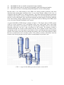
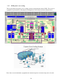
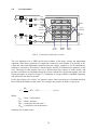
1
Advanced Pressurized Water Reactor Simulator User Manual By Cassiopeia Technologies Inc. Canada October 2011 FOREWORD Given the renewed worldwide interest in nuclear technology, there has been a growing demand for qualified nuclear professionals, which in turn has resulted in the creation of new nuclear science and technology education programs and in the growth of existing ones. Of course, this increase in the number of students pursuing nuclear degrees, has also contributed to a large need for qualified faculty and for comprehensive and up-to-date curricula. The International Atomic Energy Agency (IAEA) has established a programme in PC-based Nuclear Power Plant (NPP) simulators to assist Member States in their education and training endeavors. The objective of this programme is to provide, for a variety of nuclear reactor types, insight and practice in their operational characteristics and their response to perturbations and accident situations. To achieve this, the IAEA arranges for the supply or development of simulation programs and their associated training materials, sponsors training courses and workshops, and distributes documentation and computer programs. The simulators operate on personal computers and are provided for a broad audience of technical and nontechnical personnel as an introductory educational tool. The preferred audience, however, are faculty members interested in developing nuclear engineering courses with the support of these very effective hands-on educational tools. It is important to remember, however, that the application of these PC-based simulators is limited to providing general response characteristics of selected types of power reactor systems and that they are not intended to be used for plant-specific purposes such as design, safety evaluation, licensing or operator training. The IAEA simulator collection currently includes the following simulators: A WWER-1000 simulator provided to the IAEA by the Moscow Engineering and Physics Institute in Russia. The IAEA generic Pressurized Water Reactor (PWR) simulator has been developed by MicroSimulation Technology of USA using the PCTRAN software. This simulator is a 600 MWe generic two-loop PWR with inverted U-bend steam generators and dry containment system that could be a Westinghouse, Framatome or KWU design. The IAEA advanced PWR simulator has been developed by Cassiopeia Technologies Inc. (CTI) of Canada, and is largely based on a 600 MWe PWR design with passive safety systems, similar to the Westinghouse AP-600. The IAEA generic Boiling Water Reactor (BWR) simulator has also been developed by CTI and represents a typical 1300 MWe BWR with internal recirculation pumps and fine motion control rod drives. This simulator underwent a major enhancement effort in 2008 when a containment model based on the ABWR was added. The IAEA Pressurized Heavy Water Reactor (PHWR) simulator is also a CTI product and is largely based on the 900 MWe CANDU-9 system. The IAEA advanced PHWR simulator by CTI from Canada, which represents the ACR-700 system. The IAEA advanced BWR, which largely represents the GE ESBWR passive BWR design and was also created by CTI. This activity was initiated under the leadership of Mr. R. B. Lyon. Subsequently, Mr. J. C. Cleveland, Ms. S. Bilbao y León and later Mr. M. J. Harper and Mr. S.D. Jo from the Division of Nuclear Power became the IAEA responsible officers. More information about the IAEA simulators and the associated training is available at http://www.iaea.org/NuclearPower/Technology/Training/Simulators/ REVISIONS MADE TO IAEA PUBLICATION “ADVANCED PRESSURIZED WATER REACTOR SIMULATOR: USER MANUAL” Revisions introduced in October 2011 The entire manual was reviewed for accuracy and several minor editorial changes were introduced to improve its readability. Revisions introduced in October 2009 The entire manual was reviewed for accuracy and several minor editorial changes were introduced to improve its readability. Revisions introduced in July 2007 1. This Revision of the Passive PWR Simulator includes the thermal hydraulic model for the Passive Core Cooling Safety System based on the Westinghouse AP-600, AP-1000 Passive PWR design. However, the simulation does not claim to replicate either AP-600 or AP-1000 exactly. 2. The thermal hydraulic model includes the following processes: Primary System Natural Circulation (2x4 Loop) and heat transfer PRHR Loop Circulation (1 Loop) and heat transfer CMT Loop Circulation (2loops) Lower Containment Sump Recirculation (2 loops) for the following passive safety systems: A Passive Residual Heat Removal (PRHR) System Two Core Make-up Tanks (CMTs) A Four Stage Automatic Depressurization System (ADS) Two Accumulator Tanks (ACC) An In-containment Refueling Water Storage Tank, (IRWST) A Lower Containment Sump (CS) 3. The upgraded model is able to demonstrate the general response of these passive safety systems during a small break LOCA (SBLOCA), consistent with the sequence of events description provided for a Passive PWR. . Revisions introduced in May 2006 Due to the fact that this version of the PWR Simulator S/W incorporates intensive memory buffering for retaining trends history, some time is required for data initialization when the simulator is first loaded. To speed up this process, it is recommended that after the simulator is first loaded and the ”Plant Overview Screen” is displayed, first “RUN” the simulation for a few seconds, then “LOAD” the 100% FP IC again, before running the simulator. IAEA Passive PWR NPP Simulator Revision Details: 1. Rectify anomalies in controls for Dark and Gray rods where Gray movement is required (on small change request). Upon model testing, it was discovered that the Y-axis for the X-Y plot shown on Simulator Screen “Control/SD Rods & Reactivity” (also reference FIG. 2 in TCS-22, 2nd edition, p.14) was misrepresented. In previous version, the Y-axis plotted was : Flux Tilt Error (%) = Absolute Value [(top flux (normalized) – bottom flux(normalized))/ bottom flux (normalized) x 100 %] – deadband. Where deadband is 4 %. Thus with the above Flux Tilt Error definition, due to the Absolute Value relationship, it is no way of telling whether the flux is top-skewed, or bottom skewed. As such, this representation cannot reconcile with the respective movement of the Rods shown on the plot, and therefore the control analomies need to be rectified. In current version, the Y-axis plotted is now: Delta I = Flux tilt (%) = [(top flux (normalized) – bottom flux (normalized))/bottom flux (normalized)] x 100 %. Hence, if Delta I is +ve, the reactor flux is top skewed. Dark rods will be inserted. Similarly, if Delta I is –ve, reactor flux is bottom skewed. Dark rods will be withdrawn. There is a deadband of 4 % on either the +ve and –ve side. In order that the Dark rods will move, the flux tilt (%) has to exceed the deadband. 2. Indication of “Gray Rods Limits Reached”. In the Gray Rods control scheme, there are rod positions limits relative to reactor power as defined as follows: Reactor Power (%) 0 – 10 % 10 – 20 % 20 – 30 % 30 – 40% 40 – 50 % 50 – 60 % 60 – 70 % 70 – 80% 80 – 90 % 90 – 100 % Average Gray Rods Position (average of the rod positions for the individual four banks) 93 % - 87 % in core 87 % - 83 % in core 83 % - 70 % in core 70 % - 60 % in core 60 % - 53 % in core 53 % - 48 % in core 48 % - 44 % in core 44 % - 40 % in core 40 % - 35 % in core 35 % - 30 % in core These rod limits are designed to maintain sufficient rods reactivity worth at various power points, for power maneuvering, and as well, to maintain sufficient operating margin to allow for sudden rod insertions such as reactor power stepback, or setback, if required. Therefore, when the above defined average Gray Rods position has been reached at the specific power range, the Gray Rods will NOT be moved any more (until another power range is encountered). A flashing INDICATOR – “Gray Rods Limit Reached” will be shown on the Simulator Screen “Control/SD Rods & Reactivity” at the top right corner. If the Gray Rods Limit has been reached and the target reactor power still has not been reached, the soluble boron will be used (injection or removal) to reach the power target. As a result of the foregoing remarks, sometimes one would observe that on Simulator Screen “Control/SD Rods & Reactivity” the yellow cursor on the Reactivity Limit Diagram moves to the region where Gray rod(s) movement is required, but there are no arrows showing rods movement. Should this occur, please note the flashing INDICATOR – “Gray Rods Limit Reached”, and as well monitor the Boron load changes at that time. On occasion of large Delta T (deg. C), or large Delta I (Flux Tilt (%)), the yellow cursor will move outside the range for Reactivity Limit Diagram shown on the Simulator Screen “Control/SD Rods & Reactivity” and cannot be seen. To facilitate the user in figuring out the yellow cursor position, and hence the related Dark and Gray rods movement, digital values for Delta T and Delta I are added respectively on the X and Y axis. 3. With the loss of One Reactor Coolant Pump, implement appropriately the reactor power stepback. In the previous version of the simulator (ref. TCS-22, 2nd edition), with the loss of One Reactor Coolant Pump, there was a reactor stepback to 20 %, followed shortly by a reactor trip due to low coolant flow. This is not correct, according to one simulator user who had PWR operating experience. The stepback level should have been approximately 60 %. As well, the loss of one coolant pump should not have caused a reactor trip. These deficiencies have been corrected in this version (May 2006) of the Simulator. 4. Revise pressurizer vessel volume. In the previous model, the cross-sectional area was assumed to be 9.84 m2 (using similar data for CANDU), as the AP-600 NPP specification sheet does not contain such data. This seems to be too large, causing the liquid height to be too small, according to some users’ feedback. Now that AP-1000 Pressurizer inner diameter (2.28 m) is available, it is used to recalculate the cross-sectional area for the AP-600 pressurizer. It gives the approximate height of the vessel as 11 m, given the total volume of 45.31 m3. At full power, the liquid volume will occupy height of 7.6 m, whereas the steam volume will occupy height of 3.4 m. These data is used to revise the PWR model, until further data is obtained from Westinghouse concerning AP-600 Pressurizer dimensions. 5. Examine the need to revise the Trip Parameters to address Departure from Nucleate Boiling, and “High Steam Flow” including “All Atmospheric SRVs fail open”, and revise simulator as necessary. Two trip parameters have been added: (a) “High Steam Flow” – reactor will be tripped, when the steam flow from Steam Generator #1, OR from Steam Generator #2, exceeds 120 % of Full Power steam flow ( 644 kg/sec), OR the total steam flow from the main steam header exceeds 120 % of Full Power steam flow (1289 kg/s). (b) “DNB Trip” – Departure from Nucleate Boiling (DNB) reactor scram will occur when the average heat flux in the core exceeds 110 % of the nominal full load design value of 464 kW/m2. This is to address situation where due to loss of coolant (LOCA or loss of coolant pumps) in the core, there is insufficient cooling in core and possible hotspots (hence elevated value of heat flux) may have caused Departure from Nucleate Boiling in core.(Note: This is for instructional purposes only. Heat flux cannot be directly measured in a reactor.) 6. Review soluble Boron Controls and revise if necessary. This has been revised so that one can use the “Manual Control” to “INCREASE”, “STOP”, “DECREASE” soluble boron concentration in the core. Once the “INCREASE” (or “DECREASE”) button is pressed, the boron concentration will be increased (or decreased) continuously until “STOP” button is pressed. 7. Update screen design on all the PWR simulator screens with memory buffer. The trend history will be memorized and maintained after changing screens – 14 screens. In addition, a “AUTOSCALE” button is implemented on the “Trends Screen” so that user may enable or disable “Auto-Y-Scale” of all the 8 trends on display, at the press of the button. When “AUTOSCALE” is enabled, a red light will be turned on. 8. Update Simulator Freeze Control Design so that on simulator freeze, all the PWR screens with time trends will stop trending – 10 screens. 9. Implementation of Emergency Water Supplies to Steam Generators. In the previous version of the PWR simulator (ref. TCS-22, 2nd edition), with the insertion of Malfunction # 1 “Failed Closed All Feedwater Level Control Valves”, there will be total loss of feedwater to the steam generators #1 and #2. One will observe the expected transients of reactor trip due to Low Steam Generator Trip, followed by continuous evaporation of water (until dryout) in the steam generators due to residual heat from the core. According to one user, Emergency Water System (EWS) will be deployed to make up the loss of water inventory in the steam generators in this situation. In this version of the simulator (May 2006), Emergency Water Supply to each steam generator is implemented in the model. It will be deployed when the steam generator level drops below 5 m. This is the assumed setpoint for EWS deployment, until data is available from Westinghouse. CONTENTS 1. INTRODUCTION .................................................................................................................. 1 1.1 Purpose .......................................................................................................................... 1 1.2 Historical background ................................................................................................... 1 1.3 Prominent characteristics of PWR................................................................................. 2 2. 600 MW(e) PRESSURIZED WATER REACTOR SIMULATOR....................................... 5 2.1. Simulator startup .......................................................................................................... 7 2.2. Simulator initialization ................................................................................................. 7 2.3. List of PWR simulator display screens ........................................................................ 8 2.4. Simulator display common features ............................................................................. 8 2.5. PWR plant overview..................................................................................................... 9 2.6. PWR control loops ..................................................................................................... 10 2.7. PWR control rods and shutdown rods ........................................................................ 13 2.8. PWR reactor power control ........................................................................................ 18 2.9. PWR trip parameters .................................................................................................. 20 2.10. PWR reactor coolant system ...................................................................................... 21 2.11. PWR coolant inventory and pressurizer ..................................................................... 22 2.12. PWR coolant inventory control .................................................................................. 23 2.13. PWR coolant pressure control .................................................................................... 23 2.14. PWR turbine generator ............................................................................................... 24 2.15. PWR feedwater and extraction steam......................................................................... 25 2.16. PWR MW demand setpoint (SP) and steam generator pressure control (SGPC) ...... 26 2.17. PWR passive core cooling .......................................................................................... 28 3. PWR BASIC OPERATIONS & TRANSIENT RECOVERY ............................................. 36 3.1. 3.2. 3.3. 3.4. 3.5. Plant load maneuvering — reactor lead ..................................................................... 36 Plant load maneuvering — turbine lead ..................................................................... 38 Power level reduction to 0% FP ................................................................................. 40 Turbine trip and recovery ........................................................................................... 43 Reactor trip and recovery ........................................................................................... 44 4. PWR MALFUNCTION TRANSIENT EVENTS ................................................................ 46 4.1. Fail closed all feedwater level control valves ............................................................ 46 4.2. Steam generator #1 steam flow FT irrational ............................................................. 47 4.3. FW LCV#1 fails open................................................................................................. 47 4.4. FW LCV#1 fails closed .............................................................................................. 48 4.5. Main BFP trips ........................................................................................................... 48 4.6. Turbine throttle PT fails low ...................................................................................... 48 4.7. All atmospheric SRVs fail open ................................................................................. 49 4.8. Turbine bypass valve fails closed ............................................................................... 49 4.9. Turbine spurious trip .................................................................................................. 50 4.10. PRZR heaters #2 to # 6 turned "ON" by malfunction ................................................ 50 4.11. RC inventory feed valve (CV12) fails open ............................................................... 50 4.12. RC inventory bleed valve (CV5) fails open ............................................................... 51 4.13. PRZR pressure relief valve (CV22) fails open ........................................................... 51 4.14. One bank of dark rods drops ...................................................................................... 52 4.15. All dark rods "stuck" to MANUAL............................................................................ 52 4.16. Reactor setback/stepback both fail ............................................................................. 53 4.17. Loss of one RC pump P1 ............................................................................................ 53 4.18. Loss of 2 RC pumps in loop 1 .................................................................................... 54 4.19. 100% main steam header break .................................................................................. 54 4.20. RC hot leg #1 LOCA break ........................................................................................ 55 5. MODEL DESCRIPTION ..................................................................................................... 59 5.1. 5.2. 5.3. 5.4. 5.5. 5.6. Reactor spatial kinetic model ..................................................................................... 59 Approximation method for coupling coefficients ...................................................... 62 Summary of model formulation for PWR reactor core .............................................. 63 Coupled reactor kinetics reference ............................................................................. 71 Fuel heat transfer ........................................................................................................ 71 Core hydraulics ........................................................................................................... 72 5.6.1. Reactor coolant pumps ..................................................................................... 73 5.7. Primary coolant heat transfer...................................................................................... 74 5.8. Pressurizer .................................................................................................................. 75 5.9. Steam generators ........................................................................................................ 78 5.10. Feedwater flow ........................................................................................................... 83 5.11. Main steam system ..................................................................................................... 84 5.12. Control and protection systems .................................................................................. 85 5.12.1. Pressurizer pressure control system ............................................................... 86 5.12.2. Pressurizer level control system..................................................................... 88 5.12.3. Steam generator level control system ............................................................ 89 5.12.4. Steam generator pressure control system ....................................................... 89 5.12.5. Steam dump control system ........................................................................... 90 5.12.6. Rod control system......................................................................................... 90 5.12.7. Protection systems.......................................................................................... 91 APPENDIX: AP-600 SUMMARIZED TECHNICAL DATA ............................................... 93 1. 1.1. INTRODUCTION Purpose The International Atomic Energy Agency (IAEA) has established a programme in nuclear reactor simulation computer programs to assist its Member States in education. The objective is to provide, for a variety of advanced reactor types, insight and practice in reactor operational characteristics and their response to perturbations and accident situations. To achieve this, the IAEA arranges for the supply or development of simulation programs and materials, sponsors workshops, and distributes documentation and computer programs. This publication consists of course material for workshops on the passive pressurized water reactor (PWR) simulator. Participants in the workshops are provided with instruction and practice in using the simulator, thus gaining insight and understanding of the design and operational characteristics of passive PWR nuclear power plant systems in normal and accident situations. This manual is written with the assumption that the readers already have some knowledge of the PWR. Therefore no attempt has been made to provide detailed descriptions of each individual PWR subsystem. Those descriptions are commonly found in nuclear engineering textbooks, PWR design manuals, or IAEA technical publications. However, details are provided where necessary to describe the functionality and the interactive features of the individual simulator screen, which relates to the specific PWR subsystems. The manual covers basic NPP plant operations, like plant load maneuvering, and trips and recovery — e.g. turbine trip and reactor trip. In addition, it covers plant responses to malfunction events. Some malfunction events lead to reactor or turbine trip. Other serious malfunctions (e.g. LOCA) lead to accident situations, causing actuation of the passive core cooling safety system. It should be mentioned that the equipment and processes modeled in the simulator represent realistic PWR characteristics. However, for the purpose of the educational simulator, there are necessary simplifications and assumptions made in the models, which may not reflect any specific vendor’s design or performance. Most importantly, the responses manifested by the simulator, under accident situations, should not be used for safety analysis purposes, despite the fact that they are realistic for the purpose of educational training. As such, it is appropriate to consider that those simulator model responses perhaps only provide first order estimates of the plant transients under accident scenarios. 1.2. Historical background Pressurized water reactors were initially designed for use in submarines. The research and development work was performed by the Knolls Atomic Power Laboratory and the Westinghouse Bettis Laboratory. As a result of this initial R&D work, commercial PWRs were designed and developed for nuclear power plant applications. Eventually, several commercial PWR suppliers emerged: Westinghouse, Babcock and Wilcox; and Combustion Engineering in the USA; Siemens (Kraftwerk Union) in Germany; and Framatome in France. Subsequently, Mitsubishi in Japan and Agip Nucleari in Italy became PWR licensees. 1 Over the past three decades, many PWRs were placed in service, accumulating thousands of reactor years of operating experience. In recent years, new generations of advanced PWR nuclear power plants have been developed, building upon the past success, as well as applying lessons learned from past operating experience. The advanced PWR design features address utility and regulatory requirements. In this context, for example, important programmes in the development of advanced PWRs were initiated in the mid 1980s in the USA. In 1984, the Electric Power Research Institute (EPRI), in cooperation with US Department of Energy (DOE), and with the participation of US nuclear plant designers, and several foreign utilities, initiated a programme to develop utility requirements to guide the advanced PWR design. As a result of this effort, utilities requirements were established for large PWRs having ratings of 1200 MW(e) to 1300 MW(e), and for mid-size PWRs in the 600 MW(e) range. In the USA, the Combustion Engineering System 80+ large PWR design was certified by the U.S.NRC in 1997 and the Westinghouse AP-600 design received U.S.NRC certification in 1999. Westinghouse received U.S.NRC certification of the AP-1000 design early in 2006. The PWR simulator that accompanies this publication is largely based on a 600 MW(e) advanced PWR design, similar to the AP-600. But there are differences. The technical data sheet for AP-600, extracted from IAEA-TECDOC-1391 Status of Advanced Light Water Cooled Reactor Designs, 2004, is included in Appendix 1 for reference. Westinghouse indicates that the AP-600 has the following key features relative to earlier designs: 1. Larger core, resulting in lower power density; 2. More safety margin for DNB and LOCA; 3. Reduced worth control rods to achieve load following capability without substantial use of boron; 4. Passive core cooling system which includes core depressurization, safety injection, and residual heat removal; 5. Passive containment cooling system; 6. In-vessel retention of the molten core in the very unlikely event of a core melt accident 1.3. Prominent characteristics of the PWR concept The PWR is characterized by several prominent differences from other light water reactors (LWRs) such as the BWR: (1) (2) (3) (4) The normal core operating conditions are liquid phase water; Steam generation occurs only in the secondary phase of the power cycle, namely, the steam generators; (often referred to as “boilers” in this manual) The primary system pressure is maintained by a pressurizer that utilizes electric heaters for heating and pressurization, and sprays for cooling and depressurization; The reactor power control may be achieved by the combination of a heavy-worth bank of control rods dedicated to axial flux shape control, and reduced worth control rods position adjustments to maintain average coolant temperature during power changes. Soluble boron is only used to supplement the rod control system. Boron is dissolved in the primary system to assist in keeping the power distribution under control in the core. With such implementation of the reactor power control system, it permits a PWR to have load following operations, including frequency control, to respond to grid requirements, without substantial use of soluble boron; 2 (5) (6) (7) The PWR fuel rods are smaller and packed in larger bundles; The PWR control rods are inserted in the bundles, rather than between bundles; The entire core flow is normally pumped through the reactor coolant pumps. Because there is no bulk boiling in the PWR core during normal operations and most abnormal and normal plant transients, there is not a large density change in the core, as compared with the BWR core, during transients. This means that pressurization transients contribute little density reactivity feedback in the PWR core and consequently little power increase. On the other hand, flow coast-down transients get little negative reactivity feedback from water density change, making this type of transient, which is limiting in the PWR, most severe in terms of thermal challenge to the system. A typical 600 MW(e) PWR design is shown in Figure 1. This figure shows a PWR system with two steam generators, two recirculation loops (two return paths from each steam generator to the reactor vessel called “cold legs” and one pipe from the reactor to each steam generator called the “hot leg”.) and a pressurizer in the system. The primary coolant is circulated through the reactor coolant pumps into the lower plenum of the reactor vessel, through the reactor core from bottom to top, and out of the vessel through the upper discharge plenum. The heated water then flows through the primary side of the steam generator where the heat is transferred to the secondary system. The primary coolant is then taken from the bottom of the steam generator into the reactor coolant pumps to repeat the cycle. FIG. 1. A typical 600 MW(e) pressurized water reactor NPP. 3 The secondary coolant leaves the steam generator as saturated steam. It passes through the turbine where the energy is delivered to drive the turbine-generator unit. The remaining heat is removed in the condenser where the secondary coolant is returned to the liquid phase. From the condenser, the secondary coolant is pumped as feedwater through various heating and pumping stages until it reaches the steam generators where it picks up energy again from the primary coolant. Hence, the power cycle repeats. 4 2. 600 MW(e) PASSIVE PRESSURIZED WATER REACTOR SIMULATOR The purpose of the 600 MW(e) pressurized water reactor simulator is educational — to provide a training tool for university professors and engineers involved in teaching topics in nuclear energy. As well, nuclear engineers, scientists and trainers in the nuclear industry may find this simulator useful in broadening their understanding of PWR transients and power plant dynamics. The simulator can be executed on a personal computer (PC), to operate essentially in real time, and have a dynamic response with sufficient fidelity to provide PWR plant responses during normal operations and accident situations. It also has a user-machine interface that mimics the actual control panel instrumentation, including the plant display system, and more importantly, allows a user’s interactions with the simulator during the operation of the simulated PWR plant. The passive PWR simulator does not replicate AP-600 or AP-1000 behavior exactly. It is not intended to as the IAEA desires to remain vendor neutral. Therefore, the simulator may have design features that do not exist in either AP-600 or AP-1000. The minimum hardware configuration for the simulator consists of a Pentium PC or equivalent (minimum 1.7 GHz CPU speed), minimum of 512 Mbytes RAM , at least 30 Gbytes hard drive, 32 MB display adaptor RAM, hi-resolution video card (capable of 1024 768 resolution), 15 inch or larger high resolution SVGA colour monitor, keyboard and mouse. The operating system can be Windows 2000, or Windows XP. The requirement of having a single PC to execute the models and display the main plant parameters in real time on a high-resolution monitor implies that the models have to be as simple as possible, while having realistic dynamic response. The emphasis in developing the simulation models was on giving the desired level of realism to the user. This means being able to display all plant parameters that are critical to operating the unit, including the ones that characterize the main process, control and protective systems. The current configuration of the simulator is able to respond to the operating conditions normally encountered in power plant operations, as well as to many malfunctions, as summarized in Table I. The simulation uses a modular modeling approach: basic models for each type of device and process to be represented as algorithms and are developed in FORTRAN. These basic models are a combination of first order differential equations, logical and algebraic relations. The appropriate parameters and input-output relationships are assigned to each model as demanded by a particular system application. The interaction between the user and the simulator is via a combination of monitor displays, mouse and keyboard. Parameter monitoring and operator controls, implemented via the plant display system at the generating station, are represented in a virtually identical manner on the simulator. Control panel instruments and control devices, such as push-buttons and handswitches, are shown as stylized pictures, and are operated via special pop-up menus and dialog boxes in response to user inputs. This manual assumes that the user is familiar with the main characteristics of water cooled thermal nuclear power plants, as well as understanding the unique features of the PWR. 5 TABLE I. SUMMARY OF SIMULATOR FEATURES SYSTEM SIMULATION SCOPE REACTOR neutron flux levels over a range of 0.001 to 110% full power, 6 delayed neutron groups decay heat (3 groups) all reactivity control devices - “dark” rods; “gray” rods; boron control. Xenon/Iodine poison reactor power control system reactor shutdown system main circuit coolant loop with four pumps, two steam generators, four equivalent “lumped” reactor coolant channels pressure and inventory control which includes pressurizer, coolant letdown condenser, charge & letdown control, and pressure relief operating range is from hot zero power to full power REACTOR COOLANT STEAM & FEEDWATER steam generator dynamics, including shrink and swell effects steam supply to turbine and reheater turbine by-pass to condenser extraction steam to feed heating steam generator pressure control steam generator level control feed water system to steam generator DISPLAY PAGES OPERATOR CONTROLS MALFUNCTIONS PWR power reactor power and reactor setback and control rate of change stepback fail (input to control PWR control one bank of Dark computer) rods & control rods drop shutdown rods manual control of into the reactor core reactivity devices PWR trip - control rods and parameters boron addition/removal reactor trip reactor setback reactor stepback PWR reactor reactor coolant coolant system pumps PWR coolant coolant makeup inventory & pumps pressurizer pressurizer PWR pressure control: inventory heaters; spray; control pressure relief valve PWR pressure control pressurizer level control by regulating coolant feed & bleed flow isolation valves for coolant feed and bleed PWR feed pump on/off feedwater & operation extraction steam generator steam level controller mode: auto or manual level control setpoint during auto operation level control valve opening during manual operation extraction steam valves opening 6 Pressurizer pressure relief valve fails open charging (feed) valve fails open letdown (bleed) valve fails open pressurizer heaters #2 to # 6 turned "ON" by malfunction reactor header break all level control isolation valves fail closed one level control valve fails open one level control valve fails closed all feed pumps trip all steam safety valves open steam header break steam flow transmitter fails SYSTEM SIMULATION SCOPE DISPLAY PAGES OPERATOR CONTROLS MALFUNCTIONS simple turbine model PWR turbine turbine trip turbine spurious trip generator mechanical power and turbine run-back turbine spurious generator output are run-back turbine run-up and proportional to steam flow synchronization speeder gear and governor condenser steam valve allow synchronized discharge valves and non-synchronized operation OVERALL fully dynamic interaction PWR plant UNIT between all simulated overview systems PWR control overall unit power control loops with reactor leading mode PWR MW or turbine leading mode demand SP & unit annunciation & time steam trends generator pressure computer control of all control major system functions (SGPC) SAFETY PWR passive SYSTEM core cooling TURBINEGENERATOR 2.1. Simulator startup Select program ‘PWR’ for execution Click anywhere on ‘PWR simulator” screen Click ‘OK’ to ‘load full power IC?’ The simulator will display the ‘PWR plant overview’ screen with all parameters initialized to 100% full power At the bottom right hand corner click on ‘Run’ to start the simulator Click “IC” button to bring up the Initial Conditions pop-up window. Click “LOAD IC” and select “FP_100.ic” to be loaded, then click “RUN” to start the simulator. 2.2. Simulator initialization If at any time it is necessary to return the simulator to one of the stored initialization points, do the following: ‘Freeze’ the simulator Click on ‘IC’ Click on ‘Load IC’ Click on ‘FP_100.IC’ for 100% full power initial state Click ‘OK’ to ‘Load C:\PWR\FP_100.IC’ Click ‘YES’ to 'Load C:\PWR\FP_100.IC’ 7 Click ‘Return’ Start the simulator operating by selecting ‘Run’. 2.3. List of PWR simulator display screens (1) (2) (3) (4) (5) (6) (7) (8) (9) (10) (11) (12) (13) (14) Plant overview Control loops Control/shutdown rods & reactivity Reactor power control Trip parameters Reactor coolant system Coolant inventory & pressurizer Coolant inventory control Coolant pressure control Turbine generator Feedwater & extraction steam MW demand SP & SGPC Passive core cooling Trends 2.4. Simulator display common features The PWR simulator is made up of 14 interactive display screens or pages. All of these screens have the same information at the top and bottom of the displays, as follows: Top of the screen contains 21 plant alarms and annunciations; these indicate important status changes in plant parameters that require operator actions; Top right hand corner shows the simulator status: the window under ‘labview’ (this is the proprietary software that generates the screen displays) has a counter that is incrementing when labview is running; if labview is frozen (i.e. the displays cannot be changed) the counter will not be incrementing; the window displaying ‘CASSIM’ (this is the proprietary software that computes the simulation responses) will be green and the counter under it will not be incrementing when the simulator is frozen (i.e. the model programs are not executing), and will turn red and the counter will increment when the simulator is running; To stop (freeze) Labview click once on the ‘STOP’ sign at the top left hand corner; to restart ‘Labview’ click on the symbol at the top left hand corner; To start the simulation click on ‘Run’ at the bottom right hand corner; to ‘Stop’ the simulation click on ‘Freeze’ at the bottom right hand corner; The bottom of the screen shows the values of the following major plant parameters: Reactor neutron power (%) Reactor thermal power (%) 8 Generator output (%) Primary coolant pressure (kPa) Core flow (kg/sec) Main steam pressure (kPa) BOP(Balance of Plant) steam flow (kg/sec) The bottom left hand corner allows the initiation of two major plant events: ‘Reactor trip’ ‘Turbine trip’ these correspond to hardwired push buttons in the actual control room; The box above the Trip buttons shows the display currently selected (i.e. ‘plant overview’); by clicking and holding on the arrow in this box the titles of the other displays will be shown, and a new one can be selected by highlighting it; The remaining buttons in the bottom right hand corner allow control of the simulation one iteration at a time (‘iterate’); the selection of initialization points (‘IC’); insertion of malfunctions (‘malf’); and calling up the ‘help’ screen. (Note: The “help” screen may not be accessible) 2.5. PWR plant overview Shows a ‘line diagram’ of the main plant systems and parameters. No inputs are associated with this display. The systems and parameters displayed are as follows (starting at the bottom left hand corner): REACTOR is a 3-D spatial kinetic model with six groups of delayed neutrons; the decay heat model uses a three-group approximation; reactivity calculations include reactivity control and safety devices, Xenon, fuel temperature, moderator temperature, and Boron. The parameters displayed are: Neutron power (% full power) Reactor thermal power (% full power) Reactor coolant main loop, with four cold legs (CL1, CL2, CL3, CL4); two hot legs (HL1, HL2); pressure and inventory control systems are shown on the plant overview display, additional details will be shown on subsequent displays. The parameters displayed are: Reactor core pressure (kPa) Reactor core flow (kg/sec) Average reactor coolant temperature (C) Average fuel temperature (C) Pressurizer level (m) and pressure (kPa) Flow to/from pressurizer (kg/sec) Status of the four reactor coolant pumps (RCP#1, 2, 3, 4) The two steam generators are individually modeled, along with balance of plant systems. The parameters displayed are: Steam Generator (SG) 1, 2 level (m) 9 SG 1, 2 steam flow (kg/sec) SG 1, 2 steam pressure (kPa) SG 1, 2 steam temperature (C) Total flow (kg/sec) and opening status of the four steam relief valves (SRV’s). The four SRV’s are represented by one valve symbol - that is, in the event that any SRV opens, the valve symbol colour will be red; green when all SRV’s are closed. Moisture separator and reheater (MSR) drain flow (kg/sec) Status of control valves is indicated by their colour: green is closed, red is open Main steam governor valve status Condenser steam bypass (dump) valves status and % open Generator output (MW) is calculated from the steam flow to the turbine Condenser and condensate extraction pump (CEP) are not simulated Simulation of the feedwater system is simplified; the parameters displayed on the plant overview screen are: Total feedwater flow to the steam generators (kg/sec) Average feedwater temperature after the high pressure heaters (HPHX) Status of boiler feed pumps (FWP) is indicated as red if any pumps are ‘ON’ or green if all the pumps are ‘OFF’ Note that while the simulator is in the ‘Run’ mode, all parameters are being continually computed and all the displays are available for viewing and inputting changes. 2.6. PWR control loops The plant power control function of a PWR type nuclear power plant (NPP) is performed by two, separate control modes — one for the turbine generator, called ‘turbine leading’; and the other one for the reactor, called ‘reactor leading’. These two distinct modes of overall plant control can be switched between each other and are well coordinated for plant startup, shutdown, power operations of all kinds, and for plant upset conditions. In the ‘turbine leading’ control mode, generator power is controlled according to the power demanded by means of a remote reference value (e.g. operator input), and/or by a value derived from the actual generator frequency deviation from the grid. Using this deviation from setpoint, the reactor power is adjusted using average coolant temperature control. This mode of control is typically used for baseload operation with constant or scheduled load; as well as load following operation with a frequency control function. It is important to note that steam generator pressure is maintained constant during this control mode operation by a steam generator pressure control system that is not found on AP-600 or AP-1000. In the ‘reactor leading’ control mode, the reactor power control is determined by operator input, and/or plant upset conditions (e.g. turbine trip), which in turn will set a new average coolant temperature setpoint, hence adjusting the reactor power to match the power setpoint. The water-steam system, consisting of the turbine with its bypass system, and the steam generators, will adjust to any reactor power changes while maintaining the steam generator pressure constant with the steam generator pressure control system. 10 (1) In support of these two control modes and plant safety functions, the PWR has the following control loops as illustrated by the ‘PWR control loops screen’ in the simulator:Reactor power demand SP Reactor power demand setpoint (SP) is determined by operator input and/or by the automatic limitation functions such as the reactor stepback, which requires a step change in power reduction, or reactor setback, which requires power reduction at a fixed rate. The automatic limitation functions are triggered by specific reactor/coolant process conditions which exceed alarm setpoints. (2) Reactor power control Reactor power control in the PWR can be accomplished by core reactivity regulation and power distribution control. Core reactivity regulation accounts for reactivity changes due to power level changes, and transient xenon level resulting from the power level changes. It is achieved by a combination of control rod position adjustment, and boron concentration adjustment. The control rods that perform the core reactivity regulation are reduced strength rods, known as “Gray” rods. They are moved up or down, when the deviation between primary power (Pav) and the reference power (Pref) obtained from the turbine load (secondary power; turbine first stage pressure), exceeds the predetermined setpoint. Power distribution control is performed to maintain the core thermal margin within operating and safety limits. Power distributions, as determined by the core neutron power axial shapes, are monitored and controlled during power maneuvers. In advanced PWRs, a bank of high reactivity worth, known as ‘dark’ rods, is dedicated to axial power shape control. As the ‘dark’ rods are inserted into or withdrawn from the core, the axial power shape is bottom or top shifted respectively. Hence, with the utilization of the bank of ‘dark’ rods, axial power shape control can be accomplished. That means during power maneuvers if the axial power distribution is top skewed, insertion of ‘dark’ rods would be required. Conversely, withdrawal would be required, when the axial power distribution is bottomed skewed. (3) Control rods actuation The rod control system — ‘gray’ and ‘dark’ rods, receives rod speed and direction signals from the reactor power control system. The rod speed demand signal varies over a range depending on the input signal level. Manual control is provided to move a bank in or out at a prescribed speed. In automatic mode, the rod motion is controlled by the reactor power control system. The rods are withdrawn (or inserted) in a predetermined, programmed sequence. The shutdown banks are always held in the fully withdrawn position during normal operation, and are moved to this position at a constant speed by manual control prior to criticality. A reactor trip signal causes them to fall by gravity into the core. Only the control banks move under automatic control. Each control bank is divided into smaller groups of control rods to obtain smaller incremental reactivity changes per step. All the control rods in a group are electrically in parallel so that they move simultaneously. Individual position indication is provided for each rod. A variable speed drive provides the ability to insert small amounts of reactivity at low speeds to give fine control of reactor average coolant temperature, as well as to furnish control at high speeds to correct larger temperature transients. 11 (4) Boron control The boron concentration control system is used for relatively long term and slower core reactivity control. With the combined use of ‘gray’ and ‘dark’ rods for core reactivity regulation and core power distribution, boron concentration control is used only if necessary, so that the required rod worth is maintained for safe shutdown margin. Furthermore, the control rods are kept within rod position limitations by the control bank rod insertion limit. (5) Primary coolant pressure control Reactor coolant pressure control in the PWR is performed by the pressurizer pressure control system. This provides the capability of maintaining or restoring pressure at the design value following normal operational transients that would cause pressure changes. It is done by the control of heaters and a spray in the pressurizer. The system also provides steam relief capability by controlling the power relief valves. (6) Primary coolant inventory & makeup control The primary coolant inventory & makeup control is performed by the pressurizer level control system. It provides the capability of establishing, maintaining and restoring the pressurizer water level to the target value which is a function of the average coolant temperature. It maintains the coolant level in the pressurizer within prescribed limits by adjusting the flow of the charging (feed) and let-down (bleed) system, thus controlling the reactor coolant water inventory. (7) MW demand setpoint demand Megawatts (MW) demand setpoint is determined by operator input. This input will used as reference target for raising or lowering the turbine load. (8) Steam generator pressure control Steam generator pressure is maintained at an equilibrium, constant value determined by the heat balance between the heat input to the steam generator and the turbine steam consumption. If during power maneuvers, or plant upset, there is a mismatch between reactor thermal power and the turbine power, steam generator pressure will vary and deviate from the pressure setpoint. Under “turbine leading” control mode, control signals will be sent to the reactor power control system to reduce or increase reactor neutron power, in order that steam generator pressure will return to its setpoint. Likewise, under “reactor leading” control mode, control signals will be sent to the turbine governor control system to reduce, or raise turbine load, in order that steam generator pressure will return to its setpoint. In the event of a sudden turbine load reduction, such as abnormal load rejection, or turbine trip, where the above described control system is not fast enough to alleviate pressure changes due to such transients, an automatic steam bypass (dump) system is provided to dump the steam to the condenser, if the steam generator pressure exceeds a predetermined setpoint. (9) Steam generator level control The steam generator level control system maintains a programmed water level that is a function of turbine load. The control is a three-element controller that regulates the feedwater valve by matching feedwater flow (1st element) to steam flow (2nd element) 12 from the steam generator, while maintaining the generator level (3rd element) to its setpoint. (10) Turbine governor control The turbine governor control system will regulate the steam flow through the turbine to meet turbine load target by controlling the opening of the turbine governor valve. (11) Core cooling control The passive core cooling system uses three sources of water to maintain core cooling: (a) Core makeup tanks (CMTs) (b) Accumulators (c) In-containment refueling water storage tank (IRWST). All of these injection sources are connected directly to two nozzles on the reactor vessel. Using gravity as a motivating force, these cooling sources are designed to provide rapid cooling of the reactor core from small leaks to large loss-of-coolant accidents (LOCAs). 2.7. PWR control rods and shutdown rods The screen shows the status of the shutdown system (SDS), as well as the reactivity contributions of each device and physical phenomenon that are relevant to reactor operations. The positions of each of the two SDS SHUTDOWN ROD banks are shown relative to their normal (fully withdrawn) position. In this PWR Simulator, the reactivity worth for each SDS SHUTDOWN ROD bank is - 45.365 mk, so the total reactivity worth for the two SDS SHUTDOWN ROD banks, when fully inserted in core is - 90.73 mk. Reactivity is expressed in terms of milli-k (mk). A milli-k is equal to 0.001 in reactivity. REACTOR TRIP status is shown as NO (green) or YES (yellow), the trip can be reset here; note that SDS RESET must also be activated before the reactor power control system (RPC) will begin withdrawing the Shutdown Rods. The REACTIVITY CHANGE (mk) of each device and parameter from the initial 100% full power steady state is shown. These include: 1. SHUTDOWN RODS 2. GRAY RODS 3. DARK RODS 4. XENON 5. FUEL TEMPERATURE 6. MODERATOR TEMPERATURE & BORON Note that reactivity is a computed parameter, and not a measured parameter. It can be displayed on a simulator but is not directly available at an actual plant. Note also that when the reactor is critical, the total reactivity must be zero. This screen also shows the control rods movement diagram, and the status of the three reactivity control devices that are under the control of the reactor power control system (RPS) — gray control rods; dark control rods; boron concentration control. 13 Note that the reactivity control scheme for the control rods described below is similar to the commonly known - Mode K Reactor Control Strategy for PWR. Reference: “Automatic Reactor Power Control for a Pressurized Water Reactor“ by Jung-In Choi et al, Kyungwon University, Korea, published in Nuclear Technology Vol. 102, May 1993. The Mode K Reactor Control Strategy includes : (a) Double closed loop control of (1) reactor coolant temperature and (2) axial power difference. (b) Heavy-worth control rods bank (Dark rods) dedicated to axial shape control. (c) Light-worth control rods bank (Gray rods) for controlling coolant temperature at a reference temperature setpoint. (d) Auto regulation of both the reactivity and power distribution that permits load-follow operations (frequency control) to respond to grid conditions, with minimum use of soluble Boron. The control rods movement diagram displays the operating point in terms of flux tilt error (I) - Y axis of the diagram, and coolant temperature difference (T) - X axis of the diagram, where FLUX TILT ERROR (%), I = 100 %*(TOP FLUX - BOTTOM FLUX) / BOTTOM FLUX T = COOLANT AVERAGE TEMPERATURE Tavg - REFERENCE COOLANT TEMPERATURE Tref - TEMPERATURE DEADBAND Tdb Regions A and C in Figure 2 show cases of skewed axial power distributions - region A is top-skewed; region C is bottom skewed. The I has exceeded the target band of Idb (4%) from its reference value Iref in both regions. Hence in region A, the dark rods would be inserted to compensate for the top-skewed flux; whereas in region C, dark rods would be withdrawn to compensate for the bottom-skewed flux. 14 FIG. 2. Limit control diagram. Designating Flux Tilt error as FT (%) Average Coolant Temperature error as DT (deg. C) Region A: FT > 4; -0.5 < DT < 0.5 Region C: FT < -4; -0.5 < DT < 0.5 Region B: -4 < FT < 4; DT < -0.5 Region D: -4 < FT < 4; DT > 0.5 Region E: the four corners FT > 4; DT < -0.5; FT > 4; DT > 0.5; FT < -4; DT < -0.5; FT < -4; DT > 0.5 In this PWR simulator, there are four banks of dark rods. They are positioned near the top of the reactor core and have a strong influence on axial power shape. They move together and a few centimeters of movement are needed for effective axial power distribution control. The reactivity worth of a bank of dark rods is - 54.5 mk, so the total reactivity worth for the four banks of dark rods is - 218 mk if they are fully inserted into the core. NOTE: the four banks of Dark rods are normally controlled by the RPC system in “auto” mode. The control of dark rods can be switched to “manual” mode where each bank can be controlled individually with the control button for “IN”, “STOP”, “OUT”. 15 In regions B and D, the coolant average temperature, Tavg, exceeds the deadband Tdb (0.5 degree C) from its reference value Tref because of the change in reactivity. In region B, because Tavg is lower than Tref by the width of the deadband, gray rods would be withdrawn, one bank at a time, to increase reactivity. Conversely in region D, gray rods would be inserted, one bank at a time, to reduce reactivity, because Tavg is higher than Tref by the width of the deadband. In this PWR simulator, there are four banks of gray control rods, each bank’s reactivity worth is slightly different to enable finer reactivity control at high power: Bank #1 6.25 mk; Bank #2 - 5 mk; Bank # 3 - 3 mk; Bank # 4 - 1.75 mk. So the total reactivity worth for all the gray rods is -16 mk. For core power increase, Bank #1 gray rods will be withdrawn first, followed by Bank #2, Bank #3, and Bank #4. For core power decrease, the sequence for insertion of the banks of gray rods will be the reverse. In the event that Tavg exceeds the second deadband Tdb (1 degree C) from its reference value Tref, two banks of Gray rods would be moved simultaneously to account for the rapid change in reactivity. NOTE: The four banks of gray rods are normally controlled by the RPC system in “auto” mode. The control of gray rods can be switched to “manual” mode where each bank can be controlled individually with the control button for “IN”, “STOP”, “OUT”. In region E, both the dark rods and gray rods are used simultaneously until the core condition can be transformed into any of the A, B, C, or D regions. Then the reactivity regulation or power shape control can be obtained according to the previously described control logic of each region. It should be mentioned that in the event that the gray rods are fully withdrawn, or fully inserted, and core reactivity regulation is still required for reactor power control, the dark rods can be used in a limited way for temporary support to the gray rods. As well, the boron concentration control system can be used for relatively long term and slow core reactivity control. However, boron concentration control is used only if necessary, so that the required rod worth is maintained for safe shutdown margin, and control rods are kept within rod position limitations by the control bank rod insertion limit. AUTO/MANUAL control buttons are provided for boron control 16 In the Gray Rods control scheme, there are rod positions limits relative to reactor power as defined as follows: Reactor Power (%) 0 – 10 % 10 – 20 % 20 – 30 % 30 – 40% 40 – 50 % 50 – 60 % 60 – 70 % 70 – 80% 80 – 90 % 90 – 100 % Average Gray Rods Position (average of the rod positions for the individual four banks) 93 % - 87 % in core 87 % - 83 % in core 83 % - 70 % in core 70 % - 60 % in core 60 % - 53 % in core 53 % - 48 % in core 48 % - 44 % in core 44 % - 40 % in core 40 % - 35 % in core 35 % - 30 % in core These rod limits are specified to maintain sufficient rod reactivity worth at various power points, for power maneuvering, and for maintaining sufficient operating margin to allow for sudden rod insertions such as reactor power stepback, or setback, if required. Therefore, when the above defined average Gray Rods position has been reached at the specific power range, the Gray Rods will NOT be moved any more (until another power range is encountered). A flashing INDICATOR – “Gray Rods Limit Reached” will be shown on the Simulator Screen “Control/SD Rods & Reactivity” at the top right corner. If the Gray Rods Limit has been reached and the target reactor power still has not been reached, the soluble boron will be used (injection or removal) to reach the power target. As a result of the foregoing remarks, sometimes one would observe that on Simulator Screen “Control/SD Rods & Reactivity” the yellow cursor on the Reactivity Limit Diagram moves to the region where Gray rod(s) movement is required, but there are no arrows showing rods movement. Should this occur, please note the flashing INDICATOR – “Gray Rods Limit Reached”, and monitor the Boron load changes in the upper left hand corner of the screen at that time. On occasion of large Delta T (deg. C), or large Delta I (Flux Tilt (%)), the yellow cursor will move outside the range for Reactivity Limit Diagram shown on the Simulator Screen “Control/SD Rods & Reactivity” and cannot be seen. To facilitate the user in figuring out the yellow cursor position, and hence the related Dark and Gray rods movement, digital values for Delta T and Delta I are shown respectively on the X and Y axis. The screen also shows the reactor core normalized flux intensity map in color. The flux intensity scale is from 0 (grey color) - 1.2 (red color). The core is divided into 4 quadrants, representing 4 lumped reactor channels. Each lumped channel has 3 sections - lower core, mid-core, and upper core sections. Thus in a simplified way, the 3 dimensional reactor core can be made up of 12 core sections. Each core section’s flux intensity is represented by a color map. 17 In conjunction with the flux map of the core, the flow path of the reactor coolant through the core is also shown. Reactor coolant from the U tubes of the steam generators enters the reactor pressure vessel (RPV) at the respective cold legs entry points- CL1, CL2, CL3, CL4. The reactor coolant then travels down the core downcomer and enters into the core lower plenum, mixes with other reactor coolant streams, before entering the reactor core fuel channels. The reactor coolant carries the heat energy from the fuel pellets as it travels up the core channels, exits the core at the upper plenum, and mixes with other coolant streams before leaving the RPV at the two hot legs -HL1, HL2. 2.8. PWR reactor power control This screen permits control of the reactor power setpoint and its rate of change while under reactor power control (RPC), i.e. in ‘REACTOR LEADING’ mode. Several of the parameters key to RPC operation are displayed on this page. The status of reactor control is indicated by the four blocks marked MODE, SETBACK, STEPBACK AND SCRAM. They are normally blue but will turn red when in the abnormal state. MODE will indicate whether the reactor is under TURBINE LEADING or REACTOR LEADING control; this status can also be changed here. SETBACK status is indicated by YES or NO; setback is initiated automatically under the prescribed conditions by the RPC, but at times the operator needs to initiate a manual setback, which is done from this page on the simulator: the target value (%) and rate (%/sec) need to be input. STEPBACK status is indicated by YES or NO; stepback is initiated automatically under the prescribed conditions by the RPC, but at times the operator needs to initiate a manual stepback, which is done from this page on the simulator: the target value (%) needs to be input. SCRAM (Reactor Trip) status is indicated by YES or NO; reactor trip is initiated by the shutdown system. If the condition clears, it can be reset from here. Note however, that a tripped shutdown system must also be reset before the RPC system will pull out the shutdown rods, this must be done on the shutdown rods page Key components of RPC control algorithm are also shown on this screen. REACTOR POWER SETPOINT target and rate are specified by the user on the simulator in terms of %FP (Full Power) and %FP/sec, i.e. as linear measurements, instead of the logarithmic values used in practice. The requested rate of change should be no greater than 0.8 % of full power per second in order to avoid a reactor HIGH LOG RATE trip. This is readily achieved in the 'at-power' range (above 15%FP), but only very small rates should be used at low reactor power levels (below 1%FP), such as encountered after a reactor scram. The TURB LEAD PWR DEMAND SETPOINT is set equal to the TARGET LOAD (% FP) SETPOINT under “TURBINE LEADING” control; the upper and lower limits on this setpoint can be specified here. 18 The ACTUAL SETPOINT is set equal to the accepted “REACTOR POWER SETPOINT” TARGET under RPC control in “REACTOR LEADING” mode. HOLD POWER 'On' will select ‘REACTOR LEADING’ mode and stops any requested changes in DEMANDED POWER SETPOINT. DEMANDED RATE SETPOINT is set equal to the accepted “REACTOR POWER SETPOINT” RATE, limited by the maximum rate of 0.8 % of full power per second. DEMANDED POWER SETPOINT is the incremental power target, which is set equal to current reactor power (%) + rate (% / s) * program cycle time (sec). In this way, the DEMANDED POWER STEPOINT is “ramping” towards the REACTOR POWER SETPOINT target, at the accepted rate of change. From the DEMANDED POWER SETPOINT, a reference reactor coolant temperature (TREF) is obtained from the “Tref versus power” characteristic curve. TREF is then compared with TAVG, average coolant temperature to determine the temperature difference T. As well, the POWER ERROR is also determined from current reactor power minus demanded power setpoint. From this, the rate of change of the POWER ERROR between successive RPC program cycles will provide the “derivative” term to be used in the control algorithm. The sum of coolant temperature difference T and the power error derivative, with appropriate gains, will be used as control signal to drive the “gray” control rods, as described in previous Section 2.3. The auto/manual mode (changeable by user), rod speed, and the average position of the “gray” rods are displayed on this screen. (The AVE POS represents a %insertion of the rods into the core. In other words, an AVE POS of 7.6% means that the rods (on average) are inserted 7.6% into the core) Flux detectors are distributed throughout the reactor core to measure the average TOP FLUX (average of the flux intensity of the top four quadrants), and the average BOTTOM FLUX (average of the flux intensity of the bottom four quadrants). The difference (TOP FLUX – BOTTOM FLUX), divided by BOTTOM FLUX, times 100 % yields FLUX TILT ERROR, I, which is used as control signal to drive the “dark” rods, as described in Section 2.3. The auto/manual mode (changeable by user), rod speed, and the average position of the “dark” rods are displayed on this screen. The rate of change in reactor power is displayed, as result of the control rods movement. The following time trends are displayed: Reactor power, thermal power and turbine power (%) Coolant T error (Deg. C) Actual and demanded SP (%) Flux tilt error (%) Dark & gray rods average position in core (%) 19 Core reactivity change (K) - mk Note that the y-axis of the time trends can be changed by clicking on the max and min valves of the y-axis scale and typing in new valves. 2.9. PWR trip parameters This screen displays the parameters that cause REACTOR SCRAM, REACTOR STEPBACK, and REACTOR SETBACK. Reactor stepback is the reduction of reactor power in a large step, in response to certain process parameters exceeding alarm limits, as a measure in support of reactor safety. Reactor setback is the ramping of reactor power at fixed rate, to setback target, in response to certain process parameters exceeding alarm limits, as a measure in support of reactor safety. The TRIP PARAMETERS for REACTOR SCRAM are: Low reactor outlet header (hot legs) coolant pressure trip — trip setpoint = 14,380 kPa. Low steam generator level trip — trip setpoint = 11.94 m High reactor outlet coolant pressure trip — trip setpoint = 16,200 kPa High neutron flux trip — trip setpoint = 120 % of Neutron Flux at full power High log rate trip — trip setpoint = 8 % /s Low coolant flow trip — trip setpoint = 2,000 kg/s Low pressurizer level trip — trip setpoint = 2.7 m Low feedwater discharge header pressure — trip setpoint = 5200 kPa High Steam Flow“High Steam Flow” – reactor will be tripped, when the steam flow from Steam Generator #1, OR from Steam Generator #2, exceeds 120 % of Full Power steam flow ( 644 kg/sec), OR the total steam flow from the main steam header exceeds 120 % of Full Power steam flow (1289 kg/s). “DNB Trip” – Departure from Nucleate Boiling (DNB) reactor trip will occur when the average heat flux in the core exceeds 110 % of the nominal full load design value of 464 kW/m2. This is to address situation where due to loss of coolant (LOCA or loss of coolant pumps) in the core, there is insufficient cooling in core and possible hotspots (hence elevated value of heat flux) may have caused Departure from Nucleate Boiling in core. (Note: this trip is for instructional value only as average heat flux in the core cannot be measured directly.) Containment High Pressure Trip – reactor will be tripped when the containment pressure (which is kept at sub-atmospheric pressure) exceeds 105 kPa, in the unlikely event of a LOCA event occurring inside containment boundary. Manual trip The causes for REACTOR STEPBACK are: High reactor coolant pressure (initiated at P > 16051 kPa; target 2 % FP) Loss of one reactor coolant pump (target 60 % FP) Loss of two reactor coolant pumps (target 2 % FP) High log rate (initiated when d(lnP)/dt) > 7 %/s; target 2 % FP) Manual stepback (initiated by operator; target set by operator) 20 Hi zone flux (initiated if zone flux is > 115 % of nominal zone flux at full power) The causes for REACTOR SETBACK are: 2.10. Main steam header pressure Hi — setback if > 6150 kPa Hi pressurizer level — setback if > 12 m Manual setback in progress Low steam generator level — setback if < 12 m Low deaerator level — setback if < 2 m Hi flux tilt — setback if > 20 % Hi zonal flux — setback if > 110 % PWR reactor coolant system This screen shows a layout of the reactor coolant system (RCS): two steam generators, four recirculation loops, a pressurizer, and a letdown condenser in the system. The primary coolant is circulated through four reactor coolant pumps into the core through the lower plenum bottom of the reactor pressure vessel (RPV), through four entry points, commonly known as the “cold” legs. There is a pipe that connects one “cold” leg to the letdown condenser. Its purpose is to “bleed” off some reactor coolant from the main circuit in order to maintain inventory, if necessary, and to permit ‘clean up’ of the reactor coolant (not simulated) in the chemical and volume control system (CVS). After entering the RPV, the coolant then travels through the fuel channels in the core, and out at the top into the discharge plenum, and exits the Reactor Pressure Vessel at two exit points, commonly known as hot legs. The two hot legs are connected to two steam generators respectively. As well, there is a pipe connecting one hot leg to the pressurizer. The heated coolant then flows through the primary side (the u-tubes) of the two steam generators where the heat is transferred to the secondary system. The primary coolant is then taken from the bottom of each of the steam generator into the reactor coolant pumps (two for each steam generator) to repeat the cycle. The system components and parameters shown are: Average fuel temperature (C); average coolant temperature (C); average core flow (kg/s)); T across the core = coolant outlet temperature - coolant inlet temperature. Reactor coolant pump’s discharge flow (kg); discharge pressure (kPa); discharge temperature (C) Reactor coolant pump pop-up control which allows ‘START’, ‘STOP’ and ‘RESET’ operations Pressure (kPa), flow (kg/s) and temperature (C) at the hot legs outlet of the Reactor Pressure Vessel. Coolant flow (kg/s) to the pressurizer from one hot leg. The flow will be shown as +ve if the coolant flows from hot leg to the pressurizer; it will be shown as -ve if vice-versa. For each steam generator (SG) — feedwater flow (kg/s); feedwater level in drum (m); steam drum pressure (kPa); main steam flow from SG to main steam header (kg/s). For 21 SG1, the feed flow (kg/s) from chemical & volume control system (CVS) is shown. More explanation of this feed flow will be provided in the PWR coolant inventory & pressurizer screen. In the pressurizer, there are five electric on/off heaters, and one variable heater. They are controlled by the coolant pressure control system. The color will be red when heater is ‘on’; green when off. The following process parameters are shown: pressurizer vapor pressure (kPa); pressurizer liquid level (m); spray flow into the pressurizer (kg/s), to control pressure; pressure relief flow (kg/s) to the letdown condenser to relieve overpressure in the pressurizer. 2.11. The following time trends are displayed: The four cold legs temperatures (C) The four cold legs inflow into reactor pressure vessel (kg/s) The two hot legs pressures (kPa) The coolant feed (charging) flow (kg/s); the coolant bleed (letdown) flow (kg/s) The four cold legs pressures (kPa) Reactor power (%) PWR coolant inventory and pressurizer This screen shows the coolant pressure control system, including the pressurizer, letdown condenser, pressure relief, feed (charging) and bleed (letdown) circuits and coolant makeup storage tank. Starting with the coolant makeup storage tank at the bottom left hand corner, its level is displayed in meters. The tank supplies the flow and suction pressure for the feed (or charging) pumps P1 and P2: normally one pump is running, the pop-up menu allows START, STOP and RESET operations. The flow (kg/sec) and temperature (C) of the feed (charging) flow are displayed. The feed flow then passes through the feed isolation valve MV18 before entering Steam Generator #1, at the suction point of the reactor coolant pumps. Flow from the hot leg #1 is normally to and from the pressurizer via a short connecting pipe, a negative flow (kg/sec) indicating flow out of the pressurizer. Pressurizer pressure (kPa), temperature (C) and level (m) are displayed. Pressurizer pressure is maintained by one variable and five on-off heaters which turn ON if the pressure falls, and by pressure relief valves CV22 and CV23 if the pressure is too high. As well, coolant is drawn from connecting lines with the two cold legs (CL1 & CL2) via control valves for the purpose of spraying to depressurize the pressurizer. Parameters displayed for the letdown condenser are: pressure (kPa), temperature (C) and level (m). There is bleed (letdown) flow (kg/sec) from “cold” leg #3 via bleed (letdown) control valves CV5, CV6 and MV8, which helps maintain coolant inventory in the main coolant circuit, if the inventory becomes too high, as sensed by high pressurizer level. The outflow from the letdown condenser goes to the coolant purification system. From it, the coolant goes to the coolant makeup storage tank. 22 PRESSURIZER LEVEL SETPOINT SETPOINT are also shown. The parameters shown for the core are: average fuel temperature (C); average coolant temperature (C); core pressure at the steam generator #1 inlet plenum (kPa); average core flow (kg/s) The following time trends are displayed: and REACTOR OUTLET PRESSURE Pressurizer pressure (kPa); reactor core outlet pressure (kPa) Letdown condenser level (m); letdown condenser pressure (kPa) Pressurizer level (m) and setpoint (m) Pressurizer spray flow (kg/s) Coolant bleed (letdown) flow (kg/s); coolant feed (charging) flow (kg/s) 2.12. PWR coolant inventory control The screen shows the parameters relevant to controlling the inventory in the reactor coolant loop. Inventory control is achieved by controlling pressurizer level. Pressurizer level is normally under computer control, with the setpoint being ramped as a function of reactor power and the expected shrink and swell resulting from the corresponding temperature changes. Level control may be transferred to MANUAL and the SETPOINT can then be controlled manually. The amount of feed (charging) and bleed (letdown) is controlled about a bias value that is set to provide a steady flow of bleed to the purification system. The amount of flow may be adjusted by changing the value of the BIAS. The positions of feed (charging) and bleed (letdown) valves are normally under AUTO control, but may be changed to MANUAL using the pop-up menus. The current reactor outlet pressure is shown and the reactor outlet pressure setpoint (kPa) may be controlled manually via the pop-up menu. The following time trends are displayed: 2.13. Reactor neutron power (%); reactor thermal power (%) Reactor coolant pressure (kPa) & setpoint (kPa) Pressurizer level (m) & setpoint (m) Reactor coolant makeup feed (charging) valve position (%); reactor coolant bleed (letdown) valve position (%) PWR coolant pressure control This screen is designed to for reactor coolant pressure control: The six HEATERS are normally in AUTO, with the variable Heater (#1) modulating. The other five heaters are either ON or OFF, and under AUTO control. Via the pop-up menus MANUAL operation can be selected, and each heater may be selected to START, STOP or RESET. 23 NOTE: in order to control the variable Heater (#1) MANUALLY, one must use the pop-up menu to switch the control mode from AUTO to MANUAL first, then the control signal to the Heater #1 will be “frozen”, as shown in the numeric value display. Observe the display message above the Heater control. If it says: “MAN O/P OK”, that means Heater # 1 can now be controlled by the “MAN” pop-up menu. If it says: “MAN O/P NOT OK”, that means the MANUAL control signal from the “MAN” pop-up, and the “frozen” control signal to the Heater does not match. One must then use the “MAN” pop-up menu to enter a value equal to the “frozen” numeric value display, then the message will say “MAN O/P OK”. PRESSURIZER RELIEF VALVES CONTROL is via CV22 and CV23. These are normally in AUTO mode, but may be placed on MANUAL and the valve opening can be controlled manually via pop-up menus. PRESSURIZER SPRAY VALVES CONTROL is via SCV1 and SCV2. These are normally in AUTO mode, but may be placed on MANUAL and the valve opening can be controlled manually via pop-up menus. NOTE: in order to control the pressurizer relief valves or pressurizer spray valves MANUALLY, one must use the pop-up menu to switch the control mode from AUTO to MANUAL first, then the control signal to the control valve will be “frozen”, as shown in the numeric value display. Observe the display message above the valve control. If it says: “MAN O/P OK”, that means the control valve can now be controlled by the “MAN” pop-up menu. If it says: “MAN O/P NOT OK”, that means the MANUAL control signal from the “MAN” pop-up, and the “frozen” control signal to the control valve does not match. One must then use the “MAN” pop-up menu to enter a value equal to the “frozen” numeric value display, then the message will say “MAN O/P OK”. The current reactor outlet pressure is shown, and the reactor outlet pressure setpoint (kPa) may be controlled manually via the pop-up menu. The following time trends are displayed: 2.14. Reactor neutron power (%); reactor thermal power (%) Reactor outlet pressure (kPa) & setpoint (kPa) Pressurizer level (m) & setpoint (m) Pressurizer relief valve position (%) PWR turbine generator This screen shows the main parameters and controls associated with the turbine and the generator. The parameters displayed are: Main steam pressure (kPa) and main steam flow (kg/s); main steam stop valve (MSV) status Main steam header pressure (kPa) Status of main steam safety relief valves (SRVs) Control status (auto/manual), opening (%) and flow (kg/s) through the steam bypass valves 24 Steam flow to the turbine (kg/sec) Governor control valve position (CV) (% open) Generator output (MW); station services (MW) Turbine/generator speed of rotation (rpm) Generator breaker trip status Turbine trip status (tripped or reset) Turbine control status — auto (by computer) or manual The trend displays are: Reactor neutron & thermal power (%) Generator output (MW) Turbine steam flow (kg/s); steam BYPASS flow (kg/s) Turbine speed (RPM) Turbine governor position (%) Main steam stop valve (MSV) inlet pressure (kPa) The following pop-up menus are provided: TURBINE RUNBACK — sets target (%) and rate (%/sec) of runback when ‘accept’ is selected TURBINE TRIP STATUS — trip or reset Steam bypass valve ‘AUTO/MANUAL’ control — AUTO select allows transfer to MANUAL control, following which the manual position of the valve may be set. Computer or manual control of the turbine governor control valve (CV). Turbine runup/speedup controls 2.15. PWR feedwater and extraction steam This screen shows the portion of the feedwater system that includes the condenser, low pressure heater, deaerator, the boiler feed pumps, the high pressure heaters and associated valves, with the feedwater going to the steam generator level control valves, after leaving the HP heaters. The following display parameters and pop-up controls are provided: Main steam header pressure (kPa), steam flow through the turbine governor valve and the bypass valve (kg/s). Deaerator level (m) and deaerator pressure (kPa); extraction steam motorized valve status and controls from turbine extraction, as well pressure controller controls for main steam extraction to deaerator. The extraction steam flows (kg/s) are shown respectively for turbine extraction as well as for main steam extraction to the deaerator. Main feedwater pump and auxiliary feedwater pump status with associated pop-up menus for ‘ON/OFF’ controls. 25 HP heater motorized valves MV2 and MV3 and pop-up menus for open and close controls for controlling extraction steam flow to the HP heaters. Feedwater flow rate (kg/s) at boiler level control valve (LCV1 & LCV2) outlet and feedwater temperature (C). Pop-up controls for “auto/manual” for boiler level control valves LCV1 & LCV2 Pop-up controls for changing boiler level setpoint control from “computer SP” to “manual SP”, or vice versa. 2.16. NOTE: in order to change the boiler setpoint control from “computer SP” to “manual SP”, one must use the pop-up menu to switch the control mode from COMPUTER SP to MANUAL SP first, then the “steam generator level SP” value will be “frozen”, as shown in the numeric value display. Observe the display message next to SP control status. If it says: “MAN SP OK”, that means the boiler level SP can now be controlled by the “MAN SP” pop-up menu. If it says: “MAN SP NOT OK”, that means the MANUAL SP value from the “MAN SP” pop-up, and the “frozen” SP value (as displayed) do not match. One must then use the “MAN SP” pop-up menu to enter a value equal to the “frozen” numeric value display, then the message will say “MAN SP OK”. The following trends are displayed: Reactor neutron power (%); reactor thermal power (%); turbine power (%) Steam flow to deaerator (kg/s) Deaerator pressure (kPa) & setpoint (kPa) Main steam header pressure (kPa) High pressure heaters HX5A, HX5B extraction steam flows (kg/s) Steam generator level (m) PWR MW demand setpoint (SP) and steam generator pressure control (SGPC) This screen permits control of station load setpoint and its rate of change while under “TURBINE LEADING” control mode. Control of the main steam header pressure is also through this screen, but this is not usually changed under normal operating conditions. PWR PLANT CONTROL MODE can be changed from “REACTOR LEADING” to “TURBINE LEADING”. TARGET LOAD — on selection station load (%) and rate of change (%/sec) can be specified; change becomes effective when ‘accept’ is selected. The OPERATOR INPUT TARGET is the desired setpoint inserted by the operator; the CURRENT TARGET will be changed at a TARGET and POWER RATE specified by the operator. Note that the RANGE is only an advisory comment, numbers outside the indicated range of values may be input on the Simulator. STEAM GENERATOR PRESSURE SETPOINT CONTROL — alters the setpoint of the steam generator pressure controller, which is rarely done during power operation. Caution must be exercised when using this feature on the simulator. However, this 26 feature can be used for educational study of PWR plant responses under different secondary pressure conditions. To change SG pressure setpoint, first use the “SP Mode” pop-up to change the SP mode from “HOLD” to “INCREASE” or “DECREASE”, depending on new pressure setpoint target. After that, use the “pressure SP change rate” pop-up to enter new values for “pressure SP TARGET” (in MPa), and the “pressure SP change rate” (in MPa /minute). Observe that the SP value changes immediately, after the new SP target and rate are “accepted”. As well, the main steam header pressure shown in the display will be changed. At any time, if one wants to return the original pressure setpoint, just press the button “SP recovery” once. It can observe that the pressure SP will recover to 5740 kPa, and the main steam header pressure will follow accordingly. The following trends are provided: Reactor neutron power (%); reactor thermal power (%) Main steam header pressure (kPa) & setpoint (kPa) Current target load ( %), and turbine power (%) Steam generator 1 & 2 level (m) 27 2.17. PWR passive core cooling This screen shows the passive core cooling system in an advanced passive PWR. The screen is a graphical representation of the physical arrangement of the safety system as shown below. Note: due to screen limitation, equipment size and the respective elevation may not be in scale. 28 (1) PASSIVE SAFETY SYSTEMS With respect to thermal hydraulic phenomena, normal full-power operation is typical of most pressurized water reactor (PWR) systems. A key feature of the passive design is that it uses core decay heat to drive the core cooling process. In fact, the design uses decay heat to drive the following six natural circulation processes: • Primary System Natural Circulation (2x4 Loop) • PRHR Loop Circulation (1 Loop) • CMT Loop Circulation (2 loops) • Lower Containment Sump Recirculation (2 loops) • Containment Internal Circulation (Steam) • Containment External Circulation (Air) The passive systems in these natural circulation processes involve the following systems: • A Passive Residual Heat Removal (PRHR) System • Two Core Make-up Tanks (CMTs) • A Four Stage Automatic Depressurization System (ADS) • Two Accumulator Tanks (ACC) • An In-containment Refueling Water Storage Tank, (IRWST) • A Lower Containment Sump (CS) • Passive Containment Cooling System (PCS) Press the button “passive core cooling 3D diagram” to see the 3 dimensional layout of the passive core cooling system. (a) Passive Residual Heat Removal (PRHR) System The passive residual heat removal (PRHR) consists of a C-Tube type heat exchanger that 29 resides in the water-filled In-containment Refueling Water Storage Tank (IRWST) as shown in the schematic given in the following figure. The PRHR provides heat removal from the core via a natural circulation loop. Hot water rises through the PRHR inlet line attached to one of the hot legs. The hot water enters the tubesheet in the top header of the PRHR heat exchanger at full system pressure and temperature. The IRWST is filled with cold borated water and is open to containment. Heat removal from the PRHR heat exchanger occurs by boiling on the outside surface of the tubes. The cold primary coolant returns to the primary loop via the PRHR outline line that is connected to the steam generator lower head. The following figure illustrates the Automatic Depressurization System and all of the passive safety injection and sump recirculation flow paths and components. Figure: Passive Safety Injection and Sump Recirculation. [Note: Due to screen limitation, equipment size and respective elevation may not be in scale.] (b) Core Make-up Tank (CMT) The Core Make-up Tanks effectively replace the high-pressure safety injection systems in conventional PWRs. Each CMT consists of a large volume stainless steel tank with an inlet line that connects one of the cold legs to the top of the CMT and an outlet line that connects the bottom of the CMT to the Direct Vessel Injection (DVI) line. The DVI line is connected to the reactor vessel downcomer. Each CMT is filled with cold borated water. The CMT inlet valve is normally open and hence the CMT is normally at primary system pressure. The CMT outlet valve is normally closed, preventing natural circulation during normal operation. When 30 the outlet valve is open, a natural circulation path is established. Cold borated water flows to the reactor vessel and hot primary fluid flows upward into the top of the CMT. 31 (c) Automatic Depressurization System (ADS) The Automatic Depressurization System consists of four stages of valves that provide for the controlled reduction of primary system pressure. The first three stages consist of two trains of valves connected to the top of the pressurizer. The first stage opens on CMT liquid level. ADS stages two and three open shortly thereafter on timers. The ADS 1-3 valves discharge primary system steam into a sparger line that vents into the IRWST. The steam is condensed by direct contact with the highly subcooled water in the IRWST. The fourth stage of the ADS consists of two large valves attached to ADS lines on each hot leg. The ADS-4 valves open on low CMT liquid level and effectively bring primary side pressure down to containment conditions. The ADS-4 valves vent directly into the containment building. (d) Accumulators (ACC) The accumulators are similar to those found in conventional PWRs. They are large spherical tanks approximately three-quarters filled with cold borated water and pre-pressurized with nitrogen. The accumulator outlet line is connected to the DVI line. A pair of check valves prevents injection flow during normal operating conditions. When system pressure drops below the accumulator pressure (plus the check valve cracking pressure), the check valves open allowing coolant injection to the reactor downcomer via the DVI line.\ (e) In-containment Refueling Water Storage Tank (IRWST) The In-containment Refueling Water Storage Tank is a very large concrete pool filled with cold borated water. It serves as the heat sink for the PRHR heat exchanger and a source of water for IRWST injection. The IRWST has two injection lines connected to the reactor vessel DVI lines. These flow paths are normally isolated by two check valves in series. When the primary pressure drops below the head pressure of the water in the IRWST, the flow path is established through the DVI into the reactor vessel downcomer. The IRWST water is sufficient to flood the lower containment compartments to a level above the reactor vessel head and below the outlet of the ADS-4 lines. (f) Containment Sump Recirculation After the lower containment sump and the IRWST liquid levels are equalized, the sump valves are opened to establish a natural circulation path. Primary coolant is boiled in the reactor core by decay heat. This low-density mixture flows upward through the core and steam and liquid is vented out of the ADS-4 lines into containment. Cooler water from the containment sump is drawn in through the sump screens into the sump lines that connect to the DVI lines. 32 (g) Containment and Passive Containment Cooling System (PCCS) The following figure presents a schematic of the Passive PWR containment. It consists of a large steel vessel that houses the Nuclear Steam Supply System (NSSS) and all of the passive safety injection systems. The steel containment vessel resides inside of a concrete structure with ducts that allows cool outside air to come in contact with the outside surface of the containment vessel. When steam is vented into containment via a primary system break or ADS-4 valve actuation, it rises to the containment dome where it is condensed into liquid. The energy of the steam is transferred to the air on the outside of containment via conduction through the containment wall and natural convection to the air. As the air is heated, it rises through the ducts creating a natural circulation flow path that draws cool air in from the inlet duct and vents hot air out the top of the concrete structure. The condensate inside containment is directed back into the IRWST and the containment sump where it becomes a source of cool water in the sump recirculation process. Early in a LOCA transient, cold water is sprayed by gravity draining onto the containment vessel head to enhance containment cooling. A large tank of water, located at the top of the containment structure, serves as the source of water for this operation. 33 (2) INTEGRATED PASSIVE SAFETY SYSTEM RESPONSE DURING A SBLOCA The most effective means of describing the function of each of these passive safety systems is to relate their operation in response to a Small Break Loss-of-Coolant-Accident (SBLOCA). The first phase of a SBLOCA is the subcooled blowdown phase. During this phase, highpressure subcooled liquid is venting from the break under choked flow conditions. The primary system pressure and primary liquid inventory will be decreasing. When low pressure or low liquid level is sensed in the pressurizer, the following signals are generated: • Reactor scram • Open the PRHR inlet and outlet valves PRHR-INV and PRHR-DV • Open the CMT outlet valves: PEV1 & CMT1-DV1; PEV2 & CMT2-DV2 • Isolate Steam Generators (Feedwater and Main Steam) • Trip Reactor Coolant Pumps (Coastdown). Natural circulation is established in the PRHR loop and the CMT loops. Boiling occurs on the PRHR tubes and hot water begins to fill the top of the CMTS. If the plant continues to depressurize, eventually the primary system reaches the saturation pressure corresponding to the hot leg temperature. Depending on the break size, the system pressure will reach a plateau during which the loop will experience a period of two-phase natural circulation. 34 If primary coolant inventory continues to decrease, eventually the CMTs will begin to drain. At a predetermined CMT level (67.5%), the ADS-1 valves will open first. 80 sec after ADS-1 opens, ADS-2 will open. 80 sec after ADS-2 opens, ADS-3 will open. System pressure will drop very quickly as a result of the ADS 1-3 venting steam into the IRWST. The primary system pressure soon drops below the accumulator tank pressure and significant quantities of cold borated water are injected into the reactor vessel. If the CMT liquid level continues to decrease (below 20%), the ADS-4 actuation setpoint will be reached. The ADS-4 valves open, dropping primary system pressure below the head pressure of the IRWST liquid. The IRWST drains by gravity into the reactor vessel, out the break and ADS 4 valves into the containment sump. Eventually the IRWST and containment sump liquid levels equalize and long term sump recirculation cooling is established by opening the sump valves. Steam vented through the ADS-4 valves is condensed on the inside surfaces of the containment vessel. The containment vessel is externally cooled by air and water as needed. The condensate inside containment is returned to the containment sump and IRWST where it is available to sump recirculation cooling. 35 The screen shows the following parameters: Inside containment steel vessel — pressure (kPa); temperature (C) IRWST water temperature (C), IRWST air space pressure (kPa), IRWST level Pressurizer pressure (kPa) and level (m), and animated level shown in blue color. Water level for CMTs and accumulators. Average core flow (kg/s); average fuel temperature (C); average reactor coolant temperature (C). The screen also shows the various cooling injection flow paths during the various phases of core emergency injection, in the course of a LOCA. As described earlier, in the early phase of LOCA, natural circulation is established in the PRHR loop and the CMT loops. Boiling occurs on the PRHR tubes and hot water begins to fill the top of the CMTS. As the plant continues to depressurize, eventually the primary system reaches the saturation pressure corresponding to the hot leg temperature. Depending on the break size, the system pressure will reach a plateau during which the loop will experience a period of two-phase natural circulation. The two phase natural circulation is depicted in the coolant flow paths on the screen by various color scheme representation showing various % of quality. The injection phases shown include: (a) Cooling injection with CMTs (b) Accumulators in action (c) RCS depressurization with ADS (d) IRWST in action with long term injection (e) Sump recovery started (f) Reactor decay heat removal via PRHR HX (g) Spray from dousing tank in support of containment heat removal 36 3. 3.1. PWR BASIC OPERATIONS & TRANSIENT RECOVERY Plant load maneuvering — reactor lead POWER MANEUVER: 10 % power reduction and return to full power (1) Initialize the simulator to 100%FP. (2) Select “reactor power control” screen. (3) Run the simulator by pressing the “run” button. (4) Select the plant mode to be “REACTOR LEAD”. (5) Record in Table II the following parameters in the “full power” column, before power maneuvering. TABLE II. PLANT LOAD MANEUVERING – REACTOR LOAD Parameter Unit Reactor Neutron Power % Reactor Thermal Power % Reactor Power SP % Actual Setpoint % Demanded Power Setpoint % Demanded Rate Setpoint %/sec Current Reactor Power % Power Error % Average Coolant Temperature - Tavg C Coolant Temperature Reference - Tref C Gray rods average % (1) Full Power ____% (2) (3) (4) 90 % just 90 % return to reached stabilized 100 % stabilized 37 Comments position in core Core average top flux % Core average bottom flux % Dark rods average position in core % Boron Concentration ppm (5) Reduce power using “reactor lead power demand setpoint” pop-up. (6) Press the “reactor lead power demand setpoint” pop-up button at the bottom left corner of the screen Enter “reactor power SP target” = 90 %; enter “power rate” = 0.08 %/sec, and press “accept”. Note: due to small power rate entered (0.08%/sec), the incremental change of the Demanded Power Setpoint may not be large enough to yield a bigger than 0.5 degree of Delta T error, to move the Gray Rods. If the soluble Boron control is in AUTO, it will take action to inject Boron concentration (because Gray Rods are not moving) in order to reduce the reactor power. In case this happens, there are two choices by the users: (a) enter a faster power rate – maximum rate is 0.8 %/sec, or (b) put the Boron Control in Manual while maintaining 0.08%/sec. Observe parameter changes during transient and record comments Freeze simulator as soon as reactor neutron power just reaches 90% and record parameter values in the column (2) for “90%” power just reached. Unfreeze simulator and let parameters stabilize, record parameter values in the column (3) for “90%” power stabilized. Explain the responses for Steam generator pressure Primary coolant pressure Average coolant temperature “gray” rods and “dark” rods movement (7) Return reactor power to 100% FP at 0.08 %/sec by using the “reactor power setpoint” pop-up. See the above note regarding reactor power rate. (8) When reactor power has returned to 100 % and the parameters have stabilized, freeze and record parameter values in the column (4) of Table II “return to 100 % stabilized” (9) Note any major difference in parameter values between column (4) and column (1). Can you explain why the differences in parameter values, if any? 38 3.2. Plant load maneuvering — turbine lead POWER MANEUVER: 10% power reduction and return to full power Initialize simulator to 100% full power Verify that all parameters are consistent with full power operation. Select the MW demand SP & SGPC page Change the scale on the “reactor PWR & thermal PWR” and “current target load & turbine PWR” graphs to be between 80 and 110 percent; the “main steam Hdr pressure & SP” to 5000 and 6500 kPa, “boiler level” to 10 and 15 meters, and set “resolution” to “max out”. Record values of the parameters in the “full power” column (1) of Table III, before power maneuvering. Go to “reactor power control screen”, and record values of the parameters in the “full power” column (1) of Table IV before power maneuvering. Go back to “MW demand setpoint & SGPC” screen Reduce unit power in the ‘turbine lead’ mode, i.e. Select the plant mode to be “turbine lead” Select ‘TARGET LOAD (%)’ pop-up menu In pop-up menu lower ‘target’ to 90.00% at a ‘rate’ of 1.0 %/sec ‘accept’ and ‘return’ Observe the response of the displayed parameters until the transients in reactor power and steam pressure are completed without freezing the simulator and/or stopping labview. When the parameters have stabilized, freeze the simulator and record the parameter values in column (2) 90 % stabilized of Table III. Go to “reactor power control” screen, and record parameter values in column (2) of Table IV. 39 TABLE III. PLANT LOAD MANEUVERING – TURBINE LEAD (1) Parameter Unit Reactor Neutron Power % Reactor Thermal Power % Main Steam Header Pressure kPa Main Steam Pressure Setpoint kPa Current Target Load % Turbine Power % SG 1 Boiler Level m SG2 Boiler Level m (2) (3) (1) return to Full 90 % Power stabilized 100 % stabilized ____% Comments TABLE IV. PLANT LOAD MANEUVERING – TURBINE LEAD (2) Parameter Unit Reactor Neutron Power Reactor Thermal Power Reactor Power SP % Actual Setpoint % (1) Full Power ____% (2) 90 % stabilize d % % Demanded Power % Setpoint Demanded Rate %/sec Setpoint Current Reactor % Power Power Error % Average Coolant Temperature Tavg Coolant Temperature Reference - Tref C C 40 (4) return to 100 % stabilized Comments Gray rods average position in core Core average top flux Core average bottom flux Dark rods average position in core % Boron Load ppm % % % Explain the main changes. Why main steam header pressure rises first then drops back to the steam pressure setpoint value, although the steam pressure setpoint value is unchanged? Why steam generator’s level drops initially and then recovers? Turbine power (%) lags target load (%), but follows it nicely. However, the reactor neutron & thermal power overshoot beyond 90 % power, but recover later. But their values drift up and down for sometime before they stabilize. Recall previous power maneuvering in “reactor leading” mode, the reactor neutron & thermal power decrease orderly and do not drift as much during power changes. Can you explain why this occurs in this power maneuvering in turbine lead mode? What is the difference in the way reactor power is controlled in “reactor lead” mode, versus “turbine lead” mode ? Continuing the above operation, raise “UNIT POWER” to 100% at a rate of 1.0%FP/sec. When reactor power has returned to 100 %, and the parameters have stabilized, freeze the simulator and record the parameter values in column (3) 100 % stabilized of Table III. Go to “reactor power control” screen, and record parameters in column (3) of Table IV. Note any major difference in parameter values between column (3) and column (1). Can you explain why the differences in parameter values, if any? 3.3. Power level reduction to 0% FP Initialize the simulator to 100% FP, using “reactor lead” mode, reduce reactor power in 25% steps at 0.5%/sec During power changes, go to the following screens and record the parameters in Table V. Control rods & SD rods Reactor power control Reactor coolant system PWR inventory & pressurizer Turbine generator Feedwater & extraction steam 41 Under “comments” please note type of parameter change as a function of reactor power 0% 100%FP: constant, linear increase or decrease, non-linear increase or decrease. Note any alarms encountered during the power changes. In case reactor setback, or stepback occurs, the trip parameters screen will indicate the causes for such alarms. 42 TABLE V. Parameter POWER LEVEL REDUCTION TO 0% FP Unit 100% 75% Reactor Power % Gray rods average position % Dark Rods average position % 50% Peak Flux Tilt error during % power changes Peak T = (Tref - Tavg) C during power changes Peak reactivity change (K) mK during power changes Boron Load ppm Hot Leg 1 pressure kPa Hot Leg 2 pressure kPa Hot Leg 1 temp C Hot Leg 2 temp C Cold Leg 1 pressure kPa Cold Leg 2 pressure kPa Cold Leg 3 pressure kPa Cold Leg 4 pressure kPa Cold Leg 1 temp C Cold Leg 2 temp C Cold Leg 3 temp C Cold Leg 4 temp C Average coolant temp Tavg Average core flow C kg/s Average fuel temp C Pressurizer Level m Coolant feed (charging) flow Coolant bleed (letdown) flow SG1 Boiler Pressure kg/s kg/s SG2 Boiler Pressure kPa SG1 Boiler Level m SG2 Boiler Level m Main Steam Flow kg/s Feedwater Flow kg/s Turbine-Generator Power % 25% 0% Comments * * * kPa 43 * NOTE: it may be necessary to record these values from the relevant trend in “reactor power control” screen, or in the TRENDS screen. 3.4. Turbine trip and recovery Turbine trip transient occurs as a result of either a load rejection or turbine malfunction. On turbine trip The turbine main steam stop valves and governor valves will close, immediately shutting off steam flow to the turbine. As well, the generator breaker will trip open, causing the nominal MW power produced by the generator to drop to 0 MW almost instantly. As a result of losing MW from the generator, there is a large mismatch between the reactor thermal power and the turbine power at the boiler. This mismatch will cause a rapid increase in steam generator pressure, which will cause disturbances to the reactor coolant system. If action is not taken to reduce the reactor neutron power immediately, the boiler pressure safety relief valve will open on high boiler pressure, causing depressurization of the steam generator. This again will cause disturbances in the primary systems. To cope with the disturbances caused by the turbine trip, the plant control system is designed with the following control actions: The reactor neutron power will be reduced quickly to 60 % by rapid insertion of control rods — this is known as reactor power “stepback”. The intent is to reduce the reactor power substantially, but still maintain the reactor power at high enough level such that Xenon level buildup as a result of the stepback, will not “overcome” the positive reactivity margin available at the reactor power control system. In other words, at such reduced power level, the reactor power control system still has enough positive reactivity (from the rods) to bring the reactor back to full power, if the turbine trip can be cleared quickly. The turbine bypass valves will open automatically when turbine trip is detected, trying to alleviate steam pressure build-up. After the reactor power “stepback” has been completed, the turbine bypass valves will modulate their opening to pass sufficient steam flow to the condenser, in order to maintain boiler pressure at the constant setpoint. In this way, the turbine Bypass valves temporarily replace the turbine as the steam load, and hence eliminate the mismatch of reactor thermal power and turbine power as mentioned previously. To observe the transients as described above, using the simulator: First initialize the simulator to 100% full power, and run the simulator. Go to “reactor power control” screen; record the position of the “gray” rods and “dark” rods. Observe any flux tilt in the flux map. Go to control rods & SD rods screen”; record the flux tilt error (%), and T for the coolant temperature difference. Record the reactivity feedback effects due to Xenon (mk). Go to “turbine generator” screen; record the position of the main steam stop valve, turbine governor control valves, turbine bypass valves, boiler SRVs. 44 Record the boiler pressure, and generator output. Press the turbine trip button on the left hand bottom corner of the screen, and confirm turbine trip. 3.5. Record the position of the main steam stop valve, turbine governor control valves, turbine bypass valves, boiler SRVs. Record the reactor power, boiler pressure, and generator output, as the transient evolves. What is reactor power when turbine speed settles at 5 rpm? What is the steam flow through the bypass valve on the turbine generator screen? What is the peak boiler pressure during the transient? Go to control rods & SD rods screen; record the position of the “gray” rods and “dark” rods. How much have the gray rods moved (average position %)? How much have the dark rods moved (average position %)? Observe any flux tilt in the flux map. Go to “control/SD rods & reactivity” screen, record any flux tilt error (%), and T for the coolant temperature difference. Record the reactivity feedback effects (mk) for Xenon. What is the difference in mk for Xenon before & after the turbine trip? Go to turbine generator screen, reset turbine trip, select ‘TRU ENABLE’, and select “TRU speedup” to synchronize the generator and load to about 10 %FP. After turbine is in service, what happens to the steam bypass valve as the turbine power increases? Note the boiler pressure reading. After the turbine power is equal to the reactor power, go to the “reactor power control” screen to increase reactor power to 100 % in 25 % steps at 1 % per sec. Reactor trip and recovery Reactor trip (or reactor scram) is a reactor protective action initiated by the reactor safety shutdown system on detection of alarm limits exceeded by specific parameters in the reactor core, coolant and balance of plant systems. The parameters and the related reactor trip setpoints are described in Section 2.9 “PWR trip parameters”. Most importantly, the reactor also can be tripped by the operator MANUALLY, on account of abnormal incidents, or accidents. The reactor trip action is to drop the two banks of “shutdown” rods into the core by gravity. As well, all the “gray” rods, and the “dark” rods are also inserted into the core at maximum speed. The end result is to put lots of negative reactivity into the core such that the nuclear fission chain reaction in the core is stopped immediately. This exercise demonstrates the manual reactor trip transient, and how to recover and return the reactor to full power: 45 Initialize the simulator to 100% FP. Go to “reactor power control” screen, note the “shutdown rods” position, “gray rods” position; “dark rods” position. Go to “control/SD rods & reactivity” screen; record the reactivity mk contribution from the reactivity devices and the feedback effects — i.e. SD rods, gray rods, dark rods, Xenon, fuel temperature, moderator temperature & Boron. Manually trip the reactor using the pop-up control at the left bottom of the screen. Observe the response of the overall unit. Go to trends screen; observe the trends for reactor power, reactor coolant pressure, boiler pressure, steam flow, feedwater flow, and generator power. Wait until generator power is zero and reactor neutron power is less than 0.1%. Go to “reactor power control” screen, reset the “scram”. Go to the “control/SD & reactivity” screen and click on “SD rods reset”. Observe that the SD rods are withdrawing. As well, the dark rods are also withdrawing. Record the time (using the display under the trends) needed to withdraw all shutdown rods. Raise reactor power to 60%FP. Observe the response of the reactor regulating system and the reactivity changes that take place. 46 4. PWR MALFUNCTION TRANSIENT EVENTS Note: The PWR malfunction transient events described below are caused by malfunctions initiated in the simulator. To initiate a malfunction: Press the “MALF” button at the bottom right of any screen. A pop-up menu with a list of malfunctions will appear. Select the specific malfunction to initiate, by clicking on the malfunction item itself. The malfunction item will be highlighted in “black”. Click on “insert MF” button, if the malfunction is initiated immediately; or input a time delay (sec) in the display box, and then click “insert MF”; the malfunction will be initiated after the specified time delay has elapsed. When malfunction occurs, the “malfunction active” alarm will be “on”. To clear a malfunction which has been inserted, click on the malfunction item, and then click “clear MF”; or alternatively, click on “global clear”, which will clear all the malfunctions selected. 4.1. Fail closed all feedwater level control valves This malfunction leads to loss of feedwater to the steam generators. When this malfunction transient occurs: The boiler level drops quickly, causing low boiler level. Reactor will be setback when boiler level drops < 12m. Reactor will be tripped when boiler level drops < 11.94m. Due to loss of feedwater to the steam generators, cooling of the primary reactor coolant is reduced. The higher temperature in the reactor coolant causes it to expand. However, as the reactor is tripped, there will be rapid reduction of reactor thermal power, causing shrinkage of reactor coolant. So the net effect is the dropping of reactor coolant pressure. Dropping coolant pressure causes out-surge of coolant from the pressurizer, in order to alleviate coolant pressure decrease. Observe the flow direction in the surge line to pressurizer. As well, the electric heaters in the pressurizer will be turned on, until coolant pressure returns to its setpoint. 47 As reactor is tripped, boiler pressure is dropping rapidly, causing the turbine governor to runback the turbine - that is closing the turbine governor control valves. This results in rapid reduction of MW to zero, leading to turbine generator trip, on zero forward power. Emergency Water Supply (EWS) to each steam generator will be deployed when the steam generator level drops below 5 m. This is the assumed setpoint for EWS deployment used in this Passive PWR Simulator, but it is not based on specific design information. 4.2. Steam generator #1 steam flow FT irrational This malfunction causes steam flow transmitter for steam generator #1 to fail “low”. The consequence is that the steam generator level control system for SG#1 is “fooled” into thinking that the steam flow from SG #1 is rapidly decreasing, hence feedwater flow into SG #1 will be cutback immediately to match with “false” steam flow reduction, in an attempt to maintain the boiler level at its setpoint value. In reality, the steam flow from SG #1 remains at 100 % nominal flow rate. Because the feedwater flow is reduced to zero, by the control action of the SG level control system (SGLC), the consequence is a rapid drop in SG #1 level. When this malfunction transient occurs: Go to reactor coolant system screen, observe the steam flow from SG #1 As well, observe the feedwater flow to SG #1 Observe changes in primary coolant pressure, and the surge flow from pressurizer Reactor setback will occur first on low SG #1 level Reactor trip will occur on low-low SG #1 level Observe the coolant pressure transient, and the surge flow from pressurizer. Observe level in SG #1 As reactor is tripped, boiler pressure is dropping rapidly, causing the turbine governor to runback the turbine - that is closing the turbine governor control valves. This results in rapid reduction of MW to zero, leading to turbine generator trip, on zero forward power. 4.3. FW LCV#1 fails open This malfunction leads to maximum feedwater flow to SG #1 with the control valve LCV #1 failed wide open. Because the feedwater flow is much more than the steam flow from SG #1, as a result, the level at SG #1 is rising steadily, leading to SG # 1 high level. When this malfunction transient occurs: Go to “feedwater & extraction steam” screen; observe that LCV #1 is 100 % open. 48 Go to “reactor coolant system” screen, observe SG #1 feedwater flow, and steam flow. Note the mismatch in flow, and observe the SG #1 level. Observe if this transient has any impact to the reactor and primary coolant systems. As the boiler level very high alarm occurs, turbine generator will be tripped. When the turbine is tripped, the transient response will be similar to that described in Section 3.3 4.4. FW LCV#1 fails closed This malfunction leads to loss of feedwater to SG #1. As such, the transient response is similar to that described in Section 4.2. 4.5. Main BFP trips This malfunction leads to loss of 50 % of normal feedwater flow to SG #1 and SG #2, due to tripping of one boiler feed pump. The result is low boiler level, causing reactor setback, followed by reactor trip. The transient response is similar to that described in Section 4.1. 4.6. Turbine throttle PT fails low This malfunction causes the turbine throttle pressure transmitter to fail “low”. The consequence is that the turbine governor control system is “fooled” into thinking that the main steam pressure is rapidly decreasing, hence as a pre-programmed control action, the turbine governor will run back turbine load immediately in order to maintain main steam pressure. Because the throttle pressure transmitter has failed “low”, the turbine will be run back to 0 MW. Turbine trip will follow as a consequence of generator “zero” forward power. But in reality, the main steam pressure was never “low” in the beginning. Running back the turbine will cause immediate rise in main steam pressure. Despite the fact that the turbine Bypass valve is opening to cope with the pressure rise, it takes time for the steam pressure to decrease. The peak rise in steam pressure has immediate impact on the heat transfer of the steam generators. As a result, there will be transients on coolant temperature and pressure. But turbine trip will occur very quickly, causing large stepback of reactor power, and the transients in the reactor and primary coolant will stabilize. When this malfunction transient occurs: Go to “turbine generator” screen; observe the turbine governor position. Observe the main steam pressure transient. What is the peak steam pressure? Observe turbine power is decreased very rapidly, followed by turbine trip. Repeat this malfunction again, while the “reactor coolant system” screen is displayed. Observe the “cold” leg temperature transient. It is necessary to change the scale of the trend accordingly in order to see the transient better. What is the peak “cold” leg temperature during this malfunction? 49 4.7. Explain why the “cold” leg temperatures go up? All atmospheric SRVs fail open This malfunction will cause immediate depressurization of the steam generators. Responding to rapid dropping of main steam pressure, the turbine will be unloaded rapidly, followed by turbine trip on zero forward power. On the primary side, the rapid drop in steam generator pressure causes the coolant temperature and pressure transients, and subsequently a reactor stepback on high reactor flux. When this malfunction transient occurs: Go to “turbine generator” screen, observe the main steam safety relief valves position. Observe the turbine governor valve position, and that the turbine is unloaded rapidly. As the turbine is unloaded, observe the transient of main steam pressure. Does the turbine Bypass valve open in this transient? Repeat this transient, but this time, go to “reactor coolant system” screen first before inserting the malfunction. Observe reactor coolant temperature and pressure transient. Explain why “cold” leg temperatures are decreasing. Explain why there is a reactor stepback on high reactor flux. 4.8. Turbine bypass valve fails closed This malfunction will cause the NPP to lose its steam bypass capability, in the event of turbine trip. On turbine trip, reactor power will be stepped back automatically to 60 %. However, as a result of turbine Bypass valves failing closed, the boiler pressure will increase rapidly, causing further reactor power setback on the primary side. On the steam side, main steam safety relief valves (SRVs) will open to relieve rising main steam pressure that has exceeded the SRV’s lift setpoint. The SRVs will close on decreasing main steam pressure, and the transient stabilizes. When this malfunction transient occurs: Go to “turbine generator” screen, trip the turbine using the pop-up control at the bottom left of the screen. Observe that turbine bypass valves remain closed. Observe that Reactor power is “stepped” back. Record reactor power at the end of “stepback”. Observe the boiler pressure transient. At what pressure does the first SRV begin to open? What is the peak main steam pressure? At what pressure will all the SRVs fully reclose? Record and explain the transients in coolant temperature and pressure. 50 4.9. Turbine spurious trip This malfunction event is similar to the operational transient of turbine trip. See description in Section 3.3. 4.10. PRZR heaters #2 to # 6 turned "ON" by malfunction This malfunction event causes reactor coolant pressure to increase, due to the fact that all the pressurizer on/off heaters # 2 to #6 are turned on. The rise in coolant pressure is offset by the pressurizer spray that will come into action once the coolant pressure exceeds a predetermined setpoint for spraying. When this malfunction transient occurs: Go to “reactor coolant system” screen, observe that the pressurizer heater # 2, to # 6 are turned “on’ by malfunction. Observe that the reactor coolant pressure increases, and then the pressurizer spray comes in, to cool the pressure down. What is the net effect on reactor coolant pressure? What happens to coolant temperature - increase or decrease? Explain the response. 4.11. RC inventory feed valve (CV12) fails open This malfunction causes the reactor coolant feed (charging) flow to reach the maximum. The immediate impact to the reactor coolant system is increased coolant inventory in the system. As a result, the pressurizer level will increase, leading to increase in pressurizer pressure. This is due to the fact that the vapor space in the pressurizer has been reduced by higher liquid mass in the pressurizer because of increased inventory. The increased pressurizer pressure is offset by the spray action which comes into effect on high pressurizer pressure. But the spray will further increase the pressurizer level. The high pressurizer level will cause the inventory control system to increase the bleed (letdown) flow by opening the RC Inventory Bleed Valve CV5. As a result, the letdown condenser level will increase. Overtime, the coolant feed (charging) flow and the coolant bleed (letdown) flow will balance out, and the transient will stabilize. When this malfunction transient occurs: Go to the “coolant inventory and pressurizer” screen; observe that CV12 is 100 % open, and record the feed (charging) flow (kg/s). Observe the coolant pressure transient, and that the pressurizer spray comes in. Observe the pressurizer level and record the bleed (letdown) flow (kg/s). Observe the letdown condenser level. 51 4.12. RC inventory bleed valve (CV5) fails open This malfunction causes the reactor coolant bleed (letdown) flow to reach the maximum. As a result, the letdown condenser level will increase. The immediate impact on the reactor coolant system is decreased coolant inventory in the system. The pressurizer level will decrease, leading to decrease in pressurizer pressure. This is due to the fact that the vapor space in the pressurizer has been increased by reduced liquid mass in the pressurizer because of decreased inventory. The decreased pressurizer pressure will turn on the pressurizer heaters. The low pressurizer level will cause the inventory control system to increase the feed (charging) flow by opening the RC inventory feed valve CV12. Overtime, the coolant bleed (letdown) flow and the coolant feed (charging) flow will balance out, and the transient will stabilize. When this malfunction transient occurs: Go to the “coolant inventory and pressurizer” screen, observe that CV5 is 100 % open, and record the bleed (letdown) flow (kg/s). Observe the coolant pressure transient, and that the pressurizer heaters turn on. Observe the pressurizer level and record the feed (charging) flow (kg/s). Observe the letdown condenser level. 4.13. PRZR pressure relief valve (CV22) fails open This malfunction transient causes depressurization of the pressurizer; with steam vapor going to the letdown condenser through the failed opened pressure relief valve CV22. As the pressure is decreasing in the pressurizer, the electric heaters will be turned on. As well, pressurizer level will rise with decreasing pressure. The rising pressurizer level will cause the bleed (letdown) flow to increase, trying to reduce coolant inventory in the pressurizer. Although the electric heaters are turned on, they cannot cope with the pressure loss caused by the failed CV22 venting to the letdown condenser. As a result, the coolant pressure keeps dropping during this transient, leading to reactor trip by low reactor outlet header pressure. When this malfunction transient occurs: Go to “coolant inventory and pressurizer” screen. Observe that CV22 fails open. Observe the pressurizer pressure transient and level transient. Note that the electric heaters will turn on. Record the bleed (letdown) flow to the letdown condenser. Continue to monitor coolant pressure, record when reactor trip occurs. Monitor flow through CV22, as the pressurizer pressure continues to decrease. At what pressure will the flow from CV22 stop? Why? 52 4.14. One bank of dark rods drops This malfunction event will drop one bank of dark rods into core, imparting large negative reactivity into the core. This leads to large reduction of reactor power, and a large flux tilt towards the lower core. With a large coolant temperature error, as well as a large flux tilt error, the reactor power control (RPC) system will immediately withdraw the “gray” rods for reactivity compensation, and the “dark” rods for flux tilt compensation. However, because there is only limited reactivity available for the “gray” rods, and for the “dark” rods, even if they are fully withdrawn, their combined reactivity is insufficient to compensate for the negative reactivity imparted from dropping the bank of dark rods into core. As a result, the reactor power is decreasing; coolant pressure is decreasing. As well, the main steam pressure is decreasing, leading to turbine runback, and a subsequent turbine trip on zero forward power. The transient will evolve with the reactor power slowly decreasing to zero, due to Xenon buildup. When this malfunction transient occurs: Go to “control rods & SD rods” screen, observe that one bank of “dark” Rods has been dropped into the core. Record the overall reactivity change and reactor power, immediately after the malfunction is initiated. Note the reactor flux tilt as a consequence of this malfunction. Go to “reactor power control” screen, record the coolant temperature error, and the flux tilt error. Confirm the “gray” rods and the “dark” rods are withdrawing. Go to “reactor coolant system” screen and observe the coolant pressure transient. Go to “turbine generator” screen; observe the main steam pressure transient. Note the turbine runback is in progress. Go back to “control rods & SD rods” screen; record the overall reactivity change again. Record the reactor power. Describe and explain the long-term evolution of this transient. 4.15. All darks rods "stuck" to MANUAL This malfunction event impairs the capability of the reactor power control system to control reactor flux tilt during power maneuvering. When this malfunction transient occurs: Go to “reactor power control” screen, set the mode to “reactor lead” Enter target reactor power 70 %, and rate 0.5 % per sec. Accept the inputs. 53 Observe the coolant temperature error, and the flux tilt error, as the reactor power is decreasing to towards the target power. What is the flux tilt error when the reactor power has reached 70 %? Go to “control rods & SD rods” screen; observe the flux tilt pattern in the core. 4.16. Reactor setback/stepback both fail This malfunction event impairs the first line of protective action initiated by the reactor control system, to decrease reactor power, in response to process conditions that exceed alarm limits. However, the reactor shutdown system (SDS) is always poised to act, should those alarm limits reach the trip setpoint. Go to “control rods & SD rods” screen; insert the malfunction “reactor setback/stepback both fail”. Use the pop-up at bottom left to trip turbine. Observe that due to the malfunction, the reactor stepback cannot be initiated; therefore Control Rods will not respond to turbine trip. Record reactor power after turbine trip. Go to “turbine generator” screen; observe the main steam pressure transient. The turbine bypass valve should open to relieve steam pressure. Go to “reactor coolant system” screen; observe the transient in coolant pressure and temperature. With the reactor setback/stepback both failed, is a safety margin (e.g. coolant overpressure; fuel temperature, DNB etc.) of the system being challenged on a major transient like a turbine trip? 4.17. Loss of one RC pump P1 This malfunction event causes one primary coolant pump P1 to trip off line, due to pump failure such as rotor failure. The loss of one RC pump will immediately initiate reactor power stepback to 60 % FP.. Go to “reactor coolant system” screen; insert the malfunction for “loss of one RC Pump P1”. Observe that RC Pump 1 is tripped off, and the coolant flow is decreasing in that loop. Observe coolant flow in the other loops. Observe that reactor power is stepped back to 60 %FP. Record the reactor power after malfunction is initiated. Observe the coolant pressure and temperature transients. Repeat the malfunction event again with the use of the “reactor coolant system” screen, but before doing so, first insert malfunction for “reactor setback & stepback both failed”. The purpose is to study how the system thermal margin is challenged without the initial reactor power stepback. 54 Observe the reactor power transient, coolant pressure and temperature transients. Describe and explain the difference in responses, when compared with the previous malfunction transient. Discuss the thermal margin challenge in these cases, and how the safety and control systems can cope with these challenges. 4.18. Loss of 2 RC pumps in loop 1 This malfunction event is a more serious accident than that described in Section 4.17. Because of drastic reduction of coolant flow in one loop, the immediate effect is the cold leg temperature in loop # 1 will increase rapidly. Go to “reactor coolant system” screen; insert the malfunction for “Loss of 2 RC pumps in Loop 1”. Observe that RC Pumps 1 and 2 are tripped off, and the coolant flow is decreasing rapidly in that loop. Observe coolant flow in the other loops. Observe that reactor power is stepped back. Record the reactor power after the malfunction is initiated. Observe the coolant pressure and temperature transients. Repeat the malfunction event again with the use of the “reactor coolant system” screen, but before doing so, first insert the malfunction for “reactor setback & stepback both failed”. The purpose is to study how the system thermal margin is challenged without the initial reactor power stepback. Observe the reactor power transient, coolant pressure and temperature transients. Describe and explain the difference in responses, when compared with the previous malfunction transient. Repeat the malfunction event the third time, with the use of “reactor coolant system” screen, but before doing so, first insert malfunction for “reactor setback & stepback both failed”, and then go to “trip parameter” screen, and “DISABLE” low coolant flow trip. The purpose is again to study how the system thermal margin is further challenged without the initial reactor power stepback, AND without the reactor scram on low coolant flow. Observe the reactor power transient, coolant pressure and temperature transients. Describe and explain the difference in responses, when compared with the previous malfunction transient. Discuss the thermal margin challenge in these cases, and how the safety and control systems can cope with these challenges. 4.19. 100% main steam header break This malfunction event causes steam pipe break in the main steam line before the main steam stop valve (MSV) inside containment, leading to rapid depressurizaton of the main steam pressure. Turbine generator will be runback rapidly and will be tripped by zero forward power. The turbine trip initiates a reactor power stepback. 55 The pipe break also results in increase in steam flow from the steam generators, leading to increase in heat removal from the reactor coolant system. Therefore, coolant temperature and pressure will drop. Go to “reactor coolant system” screen; insert the malfunction “100 % main steam header break”. Observe and record the steam flows from the steam generators, and the main steam pressure. Observe the coolant temperature and pressure responses. Observe that the turbine is running back to zero power. Confirm turbine is tripped. Record reactor power after stepback. Continue to monitor coolant pressure and temperature transients. Discuss any safety margin challenge, if any, in this malfunction event, and how the safety and control systems can cope with these challenges 4.20. RC Cold Leg #4 LOCA break This malfunction event causes a “crack” opening at the cold leg #4. This break causes a loss of coolant accident (LOCA) event. Before the malfunction is inserted, it is recommended that the simulator user should be familiar with the design of the passive core injection system as described in Section 2.13 “PWR passive core cooling” screen, before performing this exercise. First load the full power initial condition (IC) and “run” the simulator. Go to “ PWR Passive Core Cooling”screen. After the screen is loaded, clickon the button “Display Trends” to bring the trend screen for PWR Passive Cooling to the front. Three trends are shown on the Trend Screen: (1) Core Flow/Total Injection Flow/Break Flow (kg/sec) (2) Reactor Coolant Pressure/ Main Steam Pressure (kPa) 56 (3) Average Fuel Temperature/ Average Coolant (Deg. C) Press the button “Display Screen” to bring the PWR Passive Core Cooling Screen to the front. In this way, one can toggle between the graphical display for Passive Core Cooling and the Trend respectively during the exercise. Now on the display for PWR Passive Core Cooling Screen, select the malfunction “RC Cold leg #4 LOCA break”, then press “insert MF”, and press “return”. Observe that the “malfunction active” alarm is “on”. Note that all the trended parameters on the screen will change immediately. Record the break flow in Table V. Record the RC coolant pressure when the reactor is scrammed. Record the parameters in Table VI during the various stages of injection: where in the system and how the two phase natural circulation occurs ? Explain Explain the RC pressure “bumps” in the course of event evolution. When do they occur? And why do they occur? 57 Explain why the accumulator is necessary? Can the accumulator be eliminated if we have a very large core makeup tank (CMT) instead? Explain why the RC depressurization by the ADS’s is necessary — to serve what purpose? 58 TABLE VI. Stages Injection of CMT service RC HOTLEG# 1 LOCA BREAK in ACC in Service RC Depress Starts IRWST in service, PRHR HX in service, Sump Recovery starts Time elapsed _____ sec _____ sec after ______ sec after _____ sec after Break after Break Break Break after Break1 Reactor Power (%) Turbine power (%) Reactor Thermal Power (%) Break Flow (kg/s) Total Injection Flow (kg/s) Core Flow (kg/s) Tavg (C) Fuel Temp (C) PRZR level (m) PRZR Pressure (kPa) Coolant Pressure at Cold Legs (kPa) Containment Pressure (kPa) Containment Temp (C) CMT Level (% full) ACC Level (% full) IRWST tank temp (C) 1 To account for the time elapsed after the break, record the CASSIM iteration counts shown at the top right hand corner, multiply that number by the time step = 0.1 sec., to get the time in seconds. This calculation has assumed that the simulation iteration starts from 0 when the LOCA malfunction is initiated. 59 5. 5.1. MODEL DESCRIPTION Reactor spatial kinetic model The reactor neutronic model for the PWR simulator is a spatial kinetic reactor model using nodal approach based on Avery's coupled region kinetics theory (section 5.4, reference 1). The reactor core is divided into a number of nodes (or zones) axially and radially. The usual considerations for the choice of the nodes are the core symmetry and the accuracy required in the description of neutron distributions, and the execution time of the nodal kinetic model. For this simulator, the PWR reactor core is divided into 12 zones: 4 zones in the upper core; 4 zones in the middle core; 4 zones in the lower core. Each zone represents a quadrant of the cross section of the core. The temporal nodal neutron population (assumed proportional to nodal power) are computed by the following nodal kinetic equations using the Avery formulation (section 5.4, Reference 1). For Zone i, 12 12 6 dN i (1 )Kij N j Ni Kij mCmj li dt j=1 j 1 m1 …..(1) dCmj mNj mCmj dt . ………….(2) Where: i, j = 1, 2, …….12 (zone number) m = 1, 2, ….6 (delayed neutron group number) Ni = Neutronic population in Zone i, respectively (nodal neutron population, considered proportional to node power) λm = Decay constants of the mth delayed neutron group β = Total delayed neutron fraction m = Delayed neutron fraction of the mth group Kij = "Coupling coefficient" determining the probability of a neutron born in zone j producing a fission neutron in zone i in the next generation. mCmj = Partial power of zone j contributed from the mth delayed neutron group. Cmj = Concentration of delayed neutron group m in zone j li = Mean neutron life time 60 Equation (1) can be rewritten by regrouping the coupling coefficients for zone i, dNi N K (1 ) Kii 1 i ii dt li li 6 C m mi m 1 6 (1 ) 12 1 12 K N K C li j 1, j i ij j li j 1, j i ij m1 m mj i 1, 2, 3. . . ..12 ...............................................(3) The above respective terms represent the various contributions of neutronic population changes in zone i from the following sources: (a) (1 ) K ii 1 Ni li is the rate of neutronic population changes in zone i due to the zone multiplication*) (b) Kii li 6 m Cmi m 1 is the rate of neutronic population changes in zone i due to its concentration of delayed neutron groups. (c) (1 ) K N li j 1, j i ij j 12 is the rate of neutronic population changes in zone i due to the coupling effects of the neutronic fluxes in the other 11 zones. (d) 12 6 1 Kij m Cmj li j 1, j i m1 is the rate of neutronic population changes in zone i due to coupling effects from the concentration of delayed neutron groups in the other 11 zones. *) ‘Zone multiplication’ is appropriate terminology to characterize the multiplicative capability of a nodal zone. 61 By introducing the definition of zone multiplication Ki = (Kii -1)/Kii, equation (3) can be written as: 6 12 dN i ( Ki ) * N i mCmi i Kij N j i dt j 1, j i m 1 12 6 1 Kij m Cmj li j 1, j i m1 …………………...(4) Where i li Kii i (1 ) li *m m li Equation (4) is almost identical to the point kinetic model for reactor zone i, with the exception of an extra zone coupling source terms: i 12 12 Kij N j j 1, j i 6 1 Kij mCmj li j 1, j i m1 and The "zone coupling effects" can be integrated into "the zone i multiplication term ii" and a metaphor for kinetic equations for zone i can be written: 12 dNi dt ( ii ij ) j 1, j i i 6 Ni m Cmi * m 1 ....……......(5) Where ii is the zone i multiplication change. ij is the net neutron multiplication change for zone i due to coupling effects in zone j Equation (4) and (5) will be identical if For zone 1 & 2, 12 N1 1 1 K12 N 2 6 1 ( K12 mCm ) l1 ZONE 2 m 1 62 For zone 1 & 3, 13 N1 1 K13 N 3 1 For zone 1 & 4, 14 m 1 N1 1 K14 N 4 1 For zone 1 & 12, 6 1 ( K13 mCm ) l1 ZONE 3 6 1 ( K14 mCm ) l1 ZONE 4 m 1 1,12 . N 1 1 1 K 1,12 N 12 6 1 ( K 1,12 m C m ) l1 ZONE 12 m 1 Repeat these similar equations for all other 11 zones. Therefore the equation for ij, the net multiplication change for zone i due to coupling effects in zone j is: ij i K ij Cm N j 1 mZONEj 1 ...........(6) N i li Ni 6 i m It can be seen that equation (6) involves the calculation of coupling coefficient Kij. These coefficients Kij define the probability of a neutron born in node j producing a fission neutron in node i in the next generation. 5.2. Approximation method for coupling coefficients In Avery's formulation (Section 5.4, reference 1), the coupling coefficients for the two energy groups of neutrons are given by the following equations: * (r ) dr (r ) (r ) dr ....................(7) k ij i th(r ) dr f th j f i i *f (r ) jth(r ) dr f * f th f Where: = fission neutron production cross section f th(r) = real thermal flux at position r *f(r) = adjoint fast flux at position r jth(r) = contribution to th(r) from fission neutrons produced in node j in the previous generation with distribution f th(r) 63 Kij involves the computation of the distribution of the real thermal flux and adjoint fast fluxes which usually involves a lot of CPU time. It would be impractical to compute these fluxes in a real-time environment. To deal with this problem, an approximate method (Section 5.4, reference 2) is implemented to compute the coupling coefficients in real time using a perturbation form (relative to the equilibrium values): K ij K ij0 g ij ..................(8) Where K ij0 = nominal value of Kij (nominal coupling coefficients) g ij = change in coupling coefficients in node i due to perturbation in node j g ij can further be defined as g ij = 14 P K k 1 k ijk ................(9) Where Pk = net multiplication perturbation in zone k (mk). K ijk = change in coupling coefficient in node i due to node j with +1.0 mk change in multiplication in node k (normalized perturbation gradient). Rewriting equation (8), 14 , K ij K ij0 Pk K ijk ................(10) k 1 It can be seen that the implementation of this approximation method involves two major components - the nominal coupling coefficients, K ij0 , and the normalized perturbation gradients, K ijk . K ij0 can be computed off-line for a given (nominal) core condition and configuration by using equation (7), for all i, j. The core is perturbed from the nominal core condition by changing net multiplication in one zone, say zone #1 and equation (7) is used again to calculate the new coupling coefficients Kij off-line, for all i, j. With the use of equation (10), K ij1 can be obtained for all i, j. Repeat the same for other zones to obtain K ijk , for k= 2, ...12. Store K ij0 and K ijk as coefficients in the computation for ij in equation (6). Equation (6) is computed every simulation iteration, and ij is obtained for all i, j and they 14 provide inputs to a summer ij , which in turn inputs into the net multiplication change j 1, j i “input” of the affected reactor zone. 64 5.3. Summary of model formulation for PWR reactor core Here is the summary of the essential modeling details for the spatial kinetic model: 12-point kinetic models are used respectively to simulate the 12 reactor zones inside the core. Each nodal kinetic model will calculate the neutron power based on 6 different neutron delay groups, and the overall change in net neutron multiplication for the zone. The change in net neutron multiplication in each zone will be a function of control devices (e.g. control rods), zonal concentration of xenon, zonal fuel temperature, zonal moderator temperature, boron concentration, reactor zones reactivity coupling effects and safety shutdown devices. The decay heat calculation within each zone assumes that 3 separate decay product groups exist, each with a different decay time constant. 3 P N FLUX ( i * N FLUX Di ) i 1 dDi i * ( i * N FLUX Di ) dt Where P = thermal power released from fuel (normalized) NFLUX = neutron population (normalized) Di = fission product concentration for Decay Group i i = fission product fraction for Decay Group i i = decay time constant for Decay Group i The decay heat from each zone is used by the “Fuel Heat Transfer to Coolant” module to calculate respective coolant temperature and fuel temperature in each zone. The reactor fuel channels are divided into 4 lumped channels. Aligned with the 4 lumped fuel channel is a “Coolant Flow Hydraulic Network”. See Figure 3 below. CL1 Channel 1 SG1 CL2 Lower Plenum CL3 SG2 Channel 2 HL1 Channel 3 Upper Plenum Channel 4 HL2 CL4 Reactor Core 65 Lower Zones Middle Upper FIG. 3. Coolant flow hydraulic network. So with this arrangement, each lumped channel “zone” (lower, middle, upper respectively) is assumed to have its own coolant flow, and its own lumped fuel element. The temperature of the lumped fuel element in each channel “zone” is calculated, and the lumped fuel sheath temperature in each “zone” will be used in the coolant heat transfer calculation. In each reactor zone, the net multiplication change includes: 1. Effects on neutron multiplication from the four banks of “Gray” Rods. The distribution of neutron absorption from control rods among the zones is dependent on the worth of the rods. As the rods are withdrawn, the upper zones have a more negative effect on neutron multiplication from the rods, hence the flux shape will be tilted towards the bottom, as the reactor power increases, as shown in Figure 4. Gray Rods Worth to Reactor Zones, as a function of Rods Position 1.2 Normalized Rods Worth 1 0.8 UPPER ZONES MIDDLE ZONES 0.6 LOWER ZONES 0.4 0.2 0 0 20 40 60 80 100 % Withdrawn from Core FIG. 4. Gray rods worth. 66 120 Dark Rods Worth to Reactor Zones, as a function of Rods Position Normalized Rods Worth 1.2 1 0.8 0.6 UPPER ZONES MIDDLE ZONES 0.4 LOWER ZONES 0.2 0 -0.2 0 20 40 60 80 100 120 % Withdrawn from Core FIG. 5. Dark rods worth. 2. Effects on neutron multiplication from the four Banks of “dark” rods. Again, the distribution of rod worth among the zones is dependent on the position of the rods. As the rods are withdrawn from their nominal positions, the influence of the rods worth in the upper zones will be more. Likewise, as the rods are inserted from their nominal position, the influence of the rods worth in the lower zones will be more. See Figure 5 for a plot of rod worth (expressed as normalized value) versus rod position (expressed as % withdrawn from core). 3. Changes in net neutron multiplication due to fuel temperature changes. D a1T f a2T f2 where a1 and a2 are constant. Tf = fuel temperature. 4. Changes in net neutron multiplication due to moderator temperature changes. 5. Changes in net neutron multiplication due to boron concentration. BD C1 C2 B C3 B 2 C4 B 4 C5Tm C6Tm2 C7Tm4 C8Tm6 C9 BTm C10 BTm3 C11Tm B 3 where Ci are constants; BD = Change in net neutron multiplication due to moderator temperature and boron concentration combined. Tm = Moderator temperature B = Boron concentration 6. Changes in net neutron multiplication due to xenon concentration. 67 7. Changes in net neutron multiplication due to zone coupling effects. (A) For each Zone Reactor, the nodal kinetic equations and the governing equations for various reactivity feedbacks are: 1. The total delayed neutron fraction is the summation of the neutron fraction of the six neutron groups 1 6 i 1 i ........................(5.3-1) 1 = total delayed neutron fraction i = group i delayed neutron fraction (i=1,2,3,4,5,6); 2. The delayed neutron groups’ concentrations can be expressed as: i * NFLUX dCi iCi TNEUTRON dt i = 1,...6 ..............(5.3-2) Ci = concentration of six delayed neutron groups, i = decay constant of delayed neutron groups. i = group i delayed neutron fraction (i=1,2,3,4,5,6) NFLUX = total neutron population in zone (norm) TNEUTRON = mean neutron lifetime (sec) 3. The rate of change of neutron population in a nodal kinetics model can be expressed as: dNFLUX ( K 1) * NFLUX 6 i1iCi dt TNEUTRON .........(5.3-3) NFLUX = total neutron population in zone (norm) TNEUTRON = mean neutron lifetime (sec) Ci = concentration of delayed neutron groups. i = decay constant of delayed neutron groups. i = group i delayed neutron fraction (i=1,2,3,4,5,6) K = overall net neutron multiplication change in nodal neutron population (K) 68 4. NFLUX can be calculated by solving the above equations, using backward Euler's expansion. NFLUX' + i 1 Ai K 1 6 i 1 Bi ) 1 t * ( TNEUTRON 6 NFLUX = where: i * Ci * t 1 i * t i * i * t Bi (1 i * t ) * TNEUTRON Ai .................(5.3-4) NFLUX' = total neutron zonal population from the previous iteration (norm) 5. The overall change in net neutron multiplication is expressed as: K = KC + KM + KB+ KXE + KSDS + KFUEL + KDIFF .........................................(5.3-5) K = overall net neutron multiplication change (K) KC = neutron net neutron multiplication change due to control devices (K) KM = overall net neutron multiplication change due to moderator temperature (K) KB = overall net neutron multiplication change due to boron concentration (K) KXE = overall net neutron multiplication change due to xenon build-up (K) KSDS = overall net neutron multiplication change due to safety shutdown systems (K) KFUEL = overall net neutron multiplication change due to fuel temperature (K) KDIFF = overall net neutron multiplication change due to coupling between zones (K) 6. The net neutron multiplication change due to control devices consist of net neutron multiplication change due to “gray” rods and “dark” rods . KC KGRAYKDARK ...............(5.3-6) KC = net neutron multiplication change due to control devices (K) 69 KGRAY = net neutron multiplication change due to “gray” rods banks (K) KDARK = net neutron multiplication change due to “dark” rods banks (K) 7. The zonal net neutron multiplication change due to xenon poisoning is assumed to be: KXE = 0.001*(27.93 - CXE)/ 12 ..............(5.3-7) KXE = overall net neutron multiplication change due to xenon poisoning (K) CXE = xenon concentration (a) It is assumed each of the 12 zones has equal contribution to the total net neutron multiplication change due to xenon poisoning. Hence there is the divider 12 in equation (5.3.7). (b) It is further assumed in (5.3.7) that at 100 % FP, the total xenon load for the overall reactor is 28 mk. This is typical 100 % FP xenon load for a generic watercooled reactor. It is not a PWR specific xenon load value. (c) Hence at 100 % FP, with xenon load at 28 mk, (5.3-7) will give KXE = 0. This is just a way of calibration for KXE at full power. One can also calibrate KXE to give –28 mk at full power, which is equally correct; but with this calibration, one has to balance this –28 mk with other means to change the net reactivity feedback effects so the overall K is zero. The formation of xenon is assumed to be from the decay of iodine as well as from the initial fission products. The concentration of xenon can be found using the following rate equations. dX X f I I X X X X ...................(5.3-8a) dt dI I f I I dt ............................................... (5.3-8b) where X, I = xenon, Iodine concentrations, nuclei/cm3 = neutron flux in neutrons/cm2.sec f = macroscopic fission cross section X , I = fractional yield of xenon and Iodine X , I = decay constants of xenon and iodine X = the microscopic capture cross-section of xenon for thermal neutrons 70 71 8. The net neutron multiplication change due to zone coupling effects: ij i K ij Cm N j 1 mZONEj 1 ............(5.3-9) N i li Ni 6 i m Where K ij K 0 ij 12 K k 1 ijk ....................(5.3-10) li Kii (1 ) i li i m * m li (See previous Section 5.2 for definition of symbols). The net neutron multiplication changes due to zone coupling effects are calculated separately for each zone. The zone coupling effects for a particular zone due to all other zones are then summed up and entered as one of the net neutron multiplication change inputs for that reactor zone. (B) The overall reactor The total power from the 12 zones reactor (each normalized) will be summed up and then divided by 12 to get the normalized overall reactor power. As well, each zonal power will provide input to the flux mapping routine for display. 72 5.4. Coupled reactor kinetics reference 1. Avery, R., “Theory of Coupled Reactors”, Proc. 2nd Int. Conf. On Peaceful Uses of Atomic Energy, Geneva, September 1958, 8/1958, p.182-191. 2. Chou, Q.B., et al, ”Development of a Low-Cost Spatial CANDU Reactor Simulation Program for Power Plant Control Studies”, Proceedings of 1975 Summer Computer Simulation Conference, San Francisco, California, July 21-23, 1975. 5.5. Fuel heat transfer The lumped parameter technique is used for calculating the heat transfer from UO2 fuel rods: T T1 r1 2 Tc r2 Cross-section of a fuel pellet, enclosed by metal fuel clad. Reactor coolant gets heat transfer from fuel clad. For fuel elements in a reactor zone, the transient fuel meat temperature and fuel clad temperature are given by: C 1 C2 dT dt 1 Q n T1 T 2 ……………(5.5-1) R1 dT 2 T T2 T2 Tc 1 ………….(5.5-2) dt R1 R2 Where Q n = nuclear heating of fuel rod r12 c p1 1 C1 = thermal capacity for fuel pellet = 2 r2 (r ) c p 2 2 C2 = thermal capacity for fuel clad = 1 R1 = resistance of UO2 and gap = 4 k 1 k1 is UO2 thermal conductivity; hg is gap conductance T1 = average fuel pellet temperature in the zone T2 = average fuel clad temperature in the zone Tc = average coolant temperature in the zone channel 73 1 2 r1 h g 5.6. Core hydraulics CL1 Channel 1 CL2 SG1 Lower Plenum CL3 Channel 2 HL1 Channel 3 Upper Plenum Channel 4 HL2 CL4 SG2 Reactor Core Lower Zones Middle Zones Upper Zones FIG. 6. Coolant flow hydraulic network. The core hydraulics for a PWR involves the solution of the mass, energy and momentum equations. Since these equations are coupled in a relatively weak fashion, it is possible to decouple the mass and momentum equations from the energy equation as far as simultaneous solution is concerned. This allows a much simpler solution of simultaneous equations in the core. Therefore for this purpose, the core is divided into flow regions or nodes axially, and pressures and flows are calculated along the reactor coolant flow regions through the core and steam generators as shown in Figure 6. Calculation of energy transfer is handled separately and is described in the next section. In the above figure, the “circles” are pressure nodes, where pressures are calculated based on the coolant mass balance at the nodes. For example, the pressure at Node 1 is given by: C N1 dPN 1 dt W IN W OUT ………………(5.6-1) Where CN1 = Node 1 Capacitance PN1 = Node 1 Pressure WIN = total flows into the node 1 WOUT = total flows out of the node 1 Similarly for all other nodes. 74 The “arrow” paths joining adjacent nodes are called “links”, where flows are calculated based on the square root of pressure difference between adjacent nodes, known as the momentum equation for incompressible flow. For example, the flow between node 1 and node 2 is given by: WN1N 2 K N1 N 2 PN1 PDYH PN 2 …………(5.6-2) Where WN1N2 = flow from node 1 to node 2 KN1N2 = flow conductance, which includes effects of valve Cv (if applicable), and effects of fluid density changes. KCV Fluid Density PN1 = Node 1 pressure PN2 = Node 2 pressure PDYH = Pump dynamic head, if applicable Similarly for all other links. By specifying the “nodes” and connecting them by “links” as in the above diagram, a nodal representation of the core hydraulic flow network problem can be defined. Then a matrix numerical method is employed to solve the system of node’s pressure equations (as in 5.6-1) and link’s momentum equations (as in 5.6-2) to obtain the pressures and flows. If the coolant heat transfer in the flow network results in fluid density changes, these changes will be taken into consideration by the link’s conductance calculations (see above KN1N2 term). 5.6.1. Reactor coolant pumps The main driving force behind the flow of coolant in the primary loops of a PWR is the reactor coolant pump. The basic formulation for the pump model is as follows: The torque balance (angular momentum) equation for the shaft and rotating assembly is: 2 d I T M T h T f …………………..(5.6.1-1) 60 dt Where I = pump moment of inertia = pump speed (RPM) TM = motor torque Th = hydraulic torque Tf = friction torque The head and torque characteristics of a pump as a function of flow rate and rotor speed, are determined using the homologous theory as given by Stepanof 1. In this theory, the pump parameters are represented by their normalized values. The shapes of the homologous curves depend only on the rated speed of the pump. The homologous modeling relates normalized 1 Stepanoff, A.J., Centrifugal and Axial Flow Pumps: Theory, Design and Application, Wiley, NY, 1957. 75 head, h, and normalized hydraulic torque, , to normalized flow, , and speed, , by tabulating: h 2 h 2 , 2 vs for 0 1 , 2 vs for 0 1 These curves are fitted with a high order polynomial function of (/), and (/) respectively, and are used by the model to compute pump head and torque. The pump head so determined is used as an input to the primary hydraulic model (equation 5.6-2). The pump torque is used as input to the torque balance equation (equation 5.6.1-1). 5.7. Primary coolant heat transfer Core fuel heat transfer starts with subcooled water flowing from “cold” legs of the steam generator, into the reactor inlet (lower) plenum. As it flows up through the core to the upper plenum, heat is transferred from the fuel channels to the coolant. The heated coolant is then recirculated to the steam generators via the hot legs. As mentioned in a previous section, each lumped channel “zone” (lower, middle, upper respectively) is assumed to have its own coolant flow, and its own lumped fuel element. The temperature of the lumped fuel element in each channel “zone” is calculated, and the lumped fuel sheath temperature in each “zone” will be used in the coolant heat transfer calculation as summarized below: The average fuel energy equation is given by: fV f C f dT f dt P UA (T f T c ) …………………(5.7-1) Where f = volume average fuel density Vf = fuel volume in one zone Cf = average fuel specific heat capacity Tf = average fuel temperature Tc = average coolant temperature P = reactor power U = overall heat transfer coefficient A = overall heat transfer area for fuel channel zone The average core coolant energy equation is given by: cVc dho Wi hi Wo ho UA(T f Tc ) …………..(5.7-2) dt 76 Where c = volume average coolant density Vc = coolant volume in one zone hi = average coolant specific enthalpy at inlet of the zone ho = average coolant specific enthalpy at outlet of the zone A = overall heat transfer area for fuel channel zone U = overall heat transfer coefficient Tf = average fuel temperature Tc = average coolant temperature Wi = coolant mass flow rate at fuel channel zone inlet Wo = coolant mass flow rate at fuel channel zone inlet The fuel heat transfer calculations (equation 5.7-1, 5.7-2) start with the lower zones, with zones inlet temperatures derived from the core lower plenum temperatures; with coolant flows derived from hydraulic flow network computation at the lower plenum. After obtaining the lower zone coolant outlet temperatures and average fuel temperatures, the calculations proceed to the middle zones, and then to the upper zones accordingly. At the core upper plenum, the coolant temperatures from the 4 lumped channels are mixed by flow turbulence, and the temperatures at the hot legs will be the coolant mixing temperatures at the upper plenum. 5.8. Pressurizer The basic pressurizer model is shown in Figure 7. It is a model designed for the educational simulator. It should be emphasized that the depth of a pressurizer model required for educational simulator differs considerably from that required for engineering or safety analysis, and therefore for this purpose, the model presented here is only a basic model. FIG. 7. Pressurizer model. 77 In steady state, the pressurizer contains steam in equilibrium with coolant fluid at saturated conditions. During transients, steam condensation or liquid flashing occurs until the equilibrium is re-established. The various properties of the two phases are obtained by applying mass and energy balance principles to the two phases separately. Taking an energy balance around the liquid phase yields the enthalpy of the liquid in the pressurizer, hl , dhl 1 wi (hi hl ) ws (hs hl ) wr (hr hl ) Q …..(5.8-1) dt ml If the pressurizer is in equilibrium, the phases would be at saturated conditions and the net mass transfer (condensate and flashing) between the two phases would be zero. Also, the total energy stored would be the sum of the total enthalpies stored in the liquid phase, the vapor phase, and the metal, respectively. The temperature of the saturated steam, tv, is obtained from the partial pressure of the steam, pv, on the saturation line: tV f 1 ( p V ) ……………..(5.8-2) The enthalpy of saturated liquid hl , and saturated steam hv, are also computed as a function of saturated steam pressure pv. hl f 2 ( pV ) ……………..(5.8-3) hV f 3 ( p V ) …..…………(5.8-4) To compute the pressurizer liquid mass, a balance is applied to the pressurizer liquid control volume space. dm l wi w s w fl w r w fv dt ……(5.8-5) The inputs to the liquid control volume are: Condensation, Wfl Insurge flow from the primary system, Wi. For outsurge flow from the pressurizer, the sign for the flow will be -ve. Spray flow, Ws 78 The outputs from the liquid control volume are: Evaporation, Wfv Pressure relief valve flow, Wr The density of the liquid, l, is computed as a function of the enthalpy of the liquid. l f 4 ( hl ) ………….(5.8-6) Liquid level is computed, knowing mass, cross sectional area and density. ll ml lA .………… (5.8-7) The steam mass is computed by applying a balance to the vapor control volume dm V w fv w r dt …………(5.8-8) The input to the steam control volume is evaporation, Wfv, while the outputs are the pressure relief flow Wr The total volume occupied by the steam vapor space is the total volume available minus the liquid volume. Vv VT ml …………….(5.8-9) l The average steam density is obtained from: v m v Vv …………….(5.8-10) The steam pressure is computed as a function of average steam density. pv f 5 ( v ) ….…………..(5.8-11) Temperature of the pressurizer liquid is computed using both pressure and enthalpy. t l f 6 ( p v , hl ) …………….(5.8-12) When the reactor coolant system is totally liquid, pressure in the pressurizer is computed as a function of a mass balance of liquid in the primary system. In summary, the basic pressurizer model on this simulator consists of solution of: three linear ordinary differential equations; six functional evaluations of the state variables using steam table. three algebraic calculations. 79 It should be mentioned that a more sophisticated model is required for engineering or safety analysis. Such enhanced modelling requires the following considerations: 5.9. the steam region could contain superheated or condensing vapor. the lower region could contain subcooled or boiling liquid. the heat transfer between the fluid and the vessel walls, as well as the interfacial heat transfer between the upper and lower regions. Mass transfer between the pressurizer regions is considered to be due to bubble rise and condensate droplets. Vapor condensation on the liquid spray will result in saturated liquid droplets reaching the liquid surface Steam generators Figure 8 shows a sketch of the typical U-tube steam generator. Primary reactor coolant enters the steam generator through the inlet plenum and flows through the U-tubes transferring heat to the secondary fluid. Secondary water enters through a feedwater ring and mixes with recirculation water as it flows downwards in the annular downcomer region. The mixture enters the subcooled region on the riser side where it is heated to saturation. As the secondary flow continues to travel upwards, boiling occurs. The steam water mixture then leaves the boiling region and passes through moisture separators (cyclones) and dryers. Saturated steam flows from the separators to the upper plenum of the dome; whereas the saturated liquid is recirculated to the downcomer. FIG. 8. Sketch of U-tube steam generator. 80 Only a summary of the main equations used in the model is provided below. (5.9-1) (5.9-3) 5.9-2 81 (5.9-4) (5.9-5) The heat transfer in the bundle zone involves three heat transfer regimes. Firstly, heat is transferred from the primary fluid to the inner side of tube metal through forced convection; secondly, heat is conducted from the inner side to the outer side of the tube by conduction; finally, heat is absorbed by the secondary fluid in the riser by natural convection. Figure 9 shows a typical grid segment of the tube bundle zone for the hot leg section. FIG. 9. Typical grid segment of the tube bundle zone. 82 Nomenclature for Figure 9: The modeling of the bundle zone dynamics (primary fluid) and that for the riser (secondary fluid) are handled as follows: 1. The primary fluid network consists of a number of flow regions - nodes belonging to the hot leg, and the cold leg. It is assumed in this model that the primary fluid is single phase, hence incompressible flow equations apply. 2. The secondary riser circuit consists of a number of flow regions - nodes. Note that the riser circuit in the hot leg, is in parallel flow direction to the primary flow; whereas the riser circuit in the cold leg is in opposite flow direction to the primary circuit. It is assumed that there is phase transition in the secondary riser circuit. 3. The pressure is calculated at each node by using mass balance at each node, and the flow between adjacent nodes is computed using a momentum balance equation in which the flow is proportional to the square root of the pressure difference. As pressures and flows are calculated for the primary nodal circuit, as well as for the secondary riser nodal circuits, the energy conservation equation is then applied for each of the primarymetal-secondary grid segments bounded by a pair of nodes in the primary circuit and an adjacent pair of nodes in the secondary circuit, as shown in the above figure. The energy conservation equations for the grid segment are as follows - 83 (5.9-6) (5.9-7) (5.9-8) (5.9-9) 84 (5.9-10) (5.9-11) (5.9-12) (5.9-13) (5.9-14) 5.10. Feedwater flow The feedwater flow is determined from the control valve position, and the pressure difference between the steam generators and the feedwater/condensate system: dw fw ( Pc Pfw Pc PSG ) c Z c fw Z fw c Z cc ( K c K fw K fwr )W fw2 dt ………. (5.10-1) 85 Where Pc = condenser pressure Pfw = feedwater pump head Pc = condensate pump head PSG = steam generator pressure Kc = loss coefficients of condensate flow Kfw = loss coefficients of feedwater flow Kfwv = loss coefficients of feedwater control valves c = density of condensate fw = density of feedwater Z c = elevation head of feedwater heater above condensate heater Z fw = elevation head of steam generator above feedwater heaters Z cc = elevation head of condenser The feedwater enthalpy is obtained from the time lag between the feedwater heater and steam generator dh fw dt h fwh h fw ………….(5.10-2) Where hfw = feedwater enthalpy at steam generator hfwh = feedwater enthalpy at feedwater heater, which is obtained from the heat balance between extraction steam from turbine for feedwater heating, and the feedwater. 5.11. Main steam system The main steam system model includes the main steam piping from the steam drum of the steam generator, the main steam isolation valve (MSV), the turbine stop valves, the turbine control valves and the condenser steam dump valves. The thermodynamic state of the main steam system is governed by conservation of energy and mass, Where Mh = total steam vapor mass in the system WSG1, WSG2 = steam flows from SG1 and SG2 to steam header 86 WT = turbine control valve flow rate WD = steam dump valve flow rate WB = steam line break flow rate The specific volume and specific internal energy are given by : The main steam pressure is determined from the equation of state (i.e. steam table look-up) : The flow between the steam generators and the main steam system has the following form: Where PSG = steam generator pressure Ph = main steam pressure KV = main steam isolating valve loss coefficient KNZ = flow restrictor loss coefficients W = steam flow rate AV = total isolation valve flow area ANZ = flow restriction throat area h = steam density The steam flow rate determined by equation (5.11-6) should not exceed choke flow conditions. Steam flow rates through the turbine valves and steam dump valves and the steam line break flow, are all assumed to be choked flow. 5.12. Control and protection systems The control systems available in this simulator include those systems as described in Section 2.2 “PWR control loops”. In this section, brief model descriptions are provided for the following systems: (1) (2) (3) (4) Pressurizer pressure control system Pressurizer level control system Steam generator three element level control system Steam generator pressure control system 87 Steam dump control system Rods Control System Protection System (5) (6) (7) 5.12.1. Pressurizer pressure control system The pressurizer pressure control system controls the pressure of the reactor coolant system at a fixed setpoint. The system consists of a combination of electric heater banks, spray valves, and relief valves actuated at the proper times by a pressure controller with PID adjustments. The pressurizer heaters are divided into two groups, consisting of one bank of variable heaters, and several banks of backup on-off heaters. The variable heaters are operated by varying the voltage applied to the heaters, thereby directly controlling their heat output over a fixed pressure range. These heaters maintain the equilibrium heat balance in the pressurizer during steady state conditions. If system pressure decreases significantly from the setpoint, the variable heaters would provide maximum heat output, and in addition, the backup heaters would be turned on. If system pressure increases above normal, all the heaters would be turned off and spray valves would be opened, proportionally over a fixed pressure range, to admit cooler water to condense steam, thereby returning system pressure to normal. Heater response is shown in Figure 10 for both variable heater, and backup heaters, Heater Output Pprop + Qback Qprop Po Poff P1 PN Pressurizer Pressures FIG. 10. Heater response. Where Qvar = variable heater maximum output Qback = backup heater maximum output 88 P2 PN = pressurizer normal pressure P2 = pressure at which variable heater output becomes zero P1 = pressure at which variable heater output becomes maximum PON = pressure setpoint to turn on the backup heaters POFF = pressure setpoint to turn off the backup heaters The total heater output, Q, is the sum of outputs of the variable and the backup heaters. Q = Q1 + Q2 ……………(5.12.1-1) Q1 = Qvar, P < P1 Q1 = 0 , P > P2 …………..(5.12.1-2) and, Q2 = Qback Q2 = 0 P > PON P < POFF ……………(5.12.1-3) The spray flow controller is modeled as: Wspray = WMIN , P < PS1 WSPRAY = WMAX, P > PS2 ……………..(5.12.1-4) Where WSPRAY = spray flow demand WMIN = minimum spray flow WMAX = maximum spray flow PS1 = pressurizer pressure corresponding to minimum spray PS2 = pressurizer pressure corresponding to maximum spray 89 Figure 11 shows the spray demand flow rate as a function of pressure. Spray flow demand WMAX WMIN Pressurizer PN PS1 PS2 FIG. 11. Spray demand flow rate. For very large pressure transients, there are power operated pressure relief valves located on the pressurizer which will open in the event that the spray valves are not capable of controlling the pressure surge. The pressure relief valve operation is expressed by an “on/off” bistable control action. In the event that a transient occurs that exceeds the capability of the pressure relief valves, spring loaded safety valves are provided on the pressurizer as a final means of protecting the integrity of the reactor coolant system. The safety valves begin to open at a given pressure setpoint and reach the fully opened position when the pressure increases by a given P. 5.12.2. Pressurizer level control system The pressurizer level control system functions to maintain the proper water inventory in the reactor coolant system. This inventory is maintained by controlling the balance between water leaving and entering the system. The water leaving the system, via piping and valves to the letdown condenser, and then to the purification and volume control system. This operation is called coolant “bleeding” or “letdown” in this simulator. The water enters the system via “charging” pumps. They are also called “feed” pumps in this simulator. Detailed descriptions are provided in the Section 2.7 “PWR coolant inventory and pressurizer”. Since letdown flow is a fixed amount, the balance is maintained by varying the charging flow as follows: Charging flow is varied by varying the position of charging flow control valves in the discharge header of the charging pumps. In this model, the charging flow control is provided by a Proportional-Integral (PI) controller, WC =WC0 +K * (e + (1/) e dt) …………..( 5.12.2-1) Where WC = charging flow rate, 90 WC0 = charging flow rate at steady state, normal pressurizer level, K = proportional gain, e = pressurizer level error, = reset (integral) time constant t = time This model assumes a linear relationship between charging pump flow rate and the charging valve position. 5.12.3. Steam generator level control system Steam generator level control is achieved through the use of the steam generator threeelement controller. The level controller is a PI reset controller adjusted to provide mostly integrating action and very little proportional signal to trim the feedwater flow. This controller has the following equation formulation: ML =KCL * (eL + (1/) eL dt) …………..( 5.12.3-1) Where ML = steam generator level controller signal to control valve KCL = proportional gain eL = steam generator level error = reset time constant Feedwater flow/steam flow controller is also a PI controller adjusted to provide mostly proportional action. MFS =KCF * (eFS + (1/) eFS dt) …………..( 5.12.3-2) Where MFS = steam generator flow controller signal to control valve KCF = proportional gain eFS = flow error = steam flow - feedwater flow = reset time constant After comparing steam flow with feedwater flow and correcting for level, the three element controller generates a total control signal M = ML + MFS to manipulate the feedwater control valve position, which eventually provides the adjusted feedwater flow rate to the steam generators. 5.12.4. Steam generator pressure control system The steam generator pressure is automatically controlled to be constant. See detailed description in Section 2.6 “ PWR control loops”. 91 For that purpose, a steam generator pressure controller (SGPC) is provided and is used to regulate the turbine inlet steam pressure by opening and closing the turbine governor control valve and the turbine bypass (or ‘steam dump’) valve, as shown in Figure 12. Currently, the steam generator pressure setpoint is set at plant design pressure of 5740 kPa. FIG. 12. Steam generator pressure control. 5.12.5. Steam dump control system The steam dump (or ‘turbine bypass’) system is to reduce excessive pressure increase and transients, and hence reduce plant trips on occasion of load rejection events. There are two modes of control. One is the steam pressure mode used during plant start-up for warming up the steam generators, and for plant shutdown, when steam generators cooldown is necessary, usually when power is less than 15 %. The second mode is the Tavg mode used at power. Tavg mode consists of turbine trip controller, which is used following a turbine trip event. The Tavg turbine trip response circuit compares the reactor coolant system Tavg to the hot shutdown (no load) Tavg. The difference signal is fed to the turbine trip controller and to two bi-stables. When the difference signal exceeds a set value, the first bi-stable will activate the first valve group. This will fully open a group of dump valves. As the difference signal increases, a second bi-stable will open more dump valves. The turbine trip controller closes all valves in sequence as the difference signal decreases. 5.12.6. Rod control system For more detailed description of the control rods system, refer to Section 2.7 “PWR control rods and shutdown rods”, and Section 2.8 ”PWR reactor power control”. This section describes the mathematical formulation of the rod control system. In this model, rod speed, or reactivity insertion, is a function of reactor power, or core average temperature (Tavg), for the case of “gray” rods. For the case of “dark” rods, the functional variable is flux tilt. In either case, the controller operates with a lead/lag element, and can be expressed as: KCR(t) = (d(KCR)/dt’) dt’ ……….(5.12.6-1) (d(KCR)/dt’) = - GCRE(t)* (CR1/CR2) + ( 1 - CR1/CR2) * t/CR2 e -t/CR2 t’ e E(t’)dt’ …..(5.12.6-2) 0 92 Where E(t) = error signal (coolant temperature, or power, or flux tilt) CR1 = lead constant (sec) CR1 = lead constant (sec) GCR = controller gain KCR(t) = control rod reactivity If the error signal is within a dead band or if the reactor is tripped, no control rod action is taken. 5.12.7. Protection systems The following reactor protection systems and trip logic are simulated in this simulator (a) Reactor trip (scram) — see Section 2.9 “PWR trip parameters” for details. (b) Reactor stepback (step reduction of reactor power) — see Section 2.5 “PWR trip parameters” for details. (c) Reactor setback (ramping down reactor power at fixed rate) — see Section 2.5 “PWR trip parameters” for details. (d) Safety passive core cooling system is actuated following: (1) Low low pressurizer level (2) Manual See Section 2.17 “PWR passive core cooling” for details. (e) (f) (g) Feedwater isolation (1) Safety passive core cooling system actuation (2) High-high steam generator level (3) Manual Turbine trip (1) Low turbine forward power (2) High-high steam generator level (3) Manual Reactor coolant pump trip (1) Manual (2) Low-low pressurizer level following reactor scram. 93 94 Appendix 1 Note: Data Sheet needs to be updated if a more up-to-date data sheet is obtained from Westinghouse AP-600 SUMMARIZED TECHNICAL DATA [Ref.: http://aris.iaea.org/ “Advanced Reactors Information System”] General plant data Reactor thermal output, (Core Power 1940 1933MWe) Power plant output, net1 600 1 Power plant efficiency, net 31% Mode of operation Baseload and load follow Plant design life 60 Plant availability target 93+ Seismic design, SSE 0.3g Primary Coolant material Water Secondary Coolant material Water Moderator material Water Thermodynamic Cycle Rankine Type of Cycle Indirect Safety goals Core damage frequency, internal events only 1.7E-07 Large release frequency, internal events only 3.0E-08 Occupational radiation exposure <0.7 Operator Action Time >0.5 Nuclear steam supply system Steam flow rate at nominal conditions 1063 Steam pressure/temperature 5.74 / 272.7 Feedwater flow rate at nominal conditions 1063 Feedwater temperature 224 Reactor coolant system Primary coolant flow rate 9940 Reactor operating pressure 15.513 Core coolant inlet temperature 279.5 Core coolant outlet temperature 315.6 Mean temperature rise across core 36.1 Reactor core Active core height 3.658 Equivalent core diameter 2.921 Average linear heat rate 13.5 Average fuel power density 28.89 Average core power density 78.82 1 MWth MWe % (baseload, load follow) Years % /RY /RY Person-Sv/RY hours kg/s MPa(a)/℃ kg/s ℃ kg/s MPa(a) ℃ ℃ ℃ m m kW/m kW/kgU MW/m3 Gross and Net plant outputs are strongly dependent on site specific characteristics, which especially impact the condenser backpressure and the amount of house loads. The values provided here are representative of US conditions with cooling towers, while the plant efficiency range provided is representative of different values observed for different site conditions and site specific design solutions. 95 Fuel material Cladding tube material Outer diameter of fuel rods Rod array of a fuel assembly Number of fuel assemblies Enrichment of reload fuel at equilibrium core Fuel cycle length Average discharge burnup of fuel Burnable absorber (strategy/material) Sintered UO2 ZIRLO™ 9.5 Square, 17x17 145 4.8 24 55000 Wet annular Burnable Absorber, Integral Fuel Burnable Absorber Control rod absorber material Ag-In-Cd (black); AG-In-Cd/304SS (gray) Soluble neutron absorber Boric Acid Reactor pressure vessel Inner diameter of cylindrical shell 3988 Wall thickness of cylindrical shell 203 Total height, inside 11708 Base material Carbon Steel Design pressure/temperature 17.1 / 343.3 Steam generator Type Delta-75, vertical, U-Tube Number 2 Total tube outside surface area 6986 Number of heat exchanger tubes 6307 Tube outside diameter 17.5 Tube material Inconel 690-TT Transport weight 365.5 Reactor coolant pump Type Seal-less Number 4 Head at rated conditions 73 Flow at rated conditions 2485 Pump speed (synchronous) 1800 Pressurizer Total volume 45.31 Steam volume: full power/zero power 14.16 Heating power of heater rods 1600 Primary containment Type Dry, free standing, steel Overall form (spherical/cylindrical) Cylindrical Dimensions (diameter/height) 39.6 / 57.6 Design pressure/temperature (DBEs) 0.316 /137.8 96 mm Wt% months MWd/kg mm mm mm MPa(a)/℃ m2 mm t m Kg/s rpm m3 m3 kW m MPa(a)/℃ Design leakage rate Is secondary containment provided? 0.12 Yes, around midannulus containment penetration area Vol%/day Residual heat removal systems Passive (see Section 3.2) Number heat exchangers 1 Type Vertical C-tube Heat transfer, design 34.5 MW Design pressure/temperature 17.1 / 343.3 MPa/ oC Safety injection systems Active/passive systems Passive (see Section 3.2) Core Makeup Tanks Number 2 Volume 56.6 m3 Design pressure/temperature 17.1 / 343.3 MPa/ oC Accumulators Number 2 Volume 56.6 m3 Design pressure/temperature 5.6/148.9 MPa/ oC In-containment Refuelling Water Storage Tank (IRWST) Number 1 Volume 1982 m3 Design pressure/temperature 0.14/65.6 MPa/ oC Turbine Type of turbines Tandem-compound 4-flow, 47 in. (1.2 m) last-stage blade Number of turbine sections per unit (e.g. 1HP / 2LP HP/MP/LP) Turbine speed 1800 (for 60Hz) or rpm 1500 (for 50Hz) Generator Type 3-phase, synchronous Rated power 880 MVA Active power, Generator Rated Output 675 MW Voltage 22 kV Frequency 50/60 Hz Condenser Type Multipressure (cooling towers) or Single pressure (direct cooling) Condenser pressure 9.1 kPa(a) Active/passive systems 97 Type Number Feedwater pumps Motor Driven 2 98