Download CS Software User Manual 1.0

CoronaScreen
A Spreadsheet Tool for the Prediction of Contaminant Plume
Length in Groundwater
Version 1.0
Software User Manual
2005
Authors: Arne Hüttmann and Steven F. Thornton
Groundwater Protection and Restoration Group
Dept of Civil and Structural Engineering
University of Sheffield
Mappin Street
Sheffield S1 3JD
United Kingdom
This user manual and the associated user guides for the models included within the CORONA Screen
decision support spreadsheet tool were prepared as part of the CORONA project, funded by the
European Commission under the Fifth Framework programme (contract number EVK1-CT-200100087).
The information contained in this user manual is copyright to the authors
Contents
1. Purpose of this User-Manual................................................................................................. 1
2. Software Requirements.......................................................................................................... 1
3. Installation .............................................................................................................................. 1
4. Settings and Add-Ins.............................................................................................................. 1
5. The Spreadsheet ..................................................................................................................... 2
5.1 Welcome sheet ................................................................................................................... 2
5.2 Introduction sheet............................................................................................................... 2
5.3 Data Input sheet.................................................................................................................. 3
5.3.1 Sections on Data Input ................................................................................................ 4
5.3.2 Dialogs related to the Data Input worksheet .............................................................. 5
5.4 Electron Balance Model sheet............................................................................................ 7
5.5 Analytical Model sheet....................................................................................................... 7
5.6 Travelling 1D Model sheet................................................................................................. 8
5.7 Print Summary sheet .......................................................................................................... 8
6. Comment on Calculations ..................................................................................................... 8
7. Troubleshooting...................................................................................................................... 9
8. Help and Support ................................................................................................................... 9
9. References ............................................................................................................................. 10
Appendix I. Example inputs for addition of new contaminants .......................................... 10
i
1. Purpose of this User-Manual
This document explains how to install and use CoronaScreen. The requirements for the model to run, its
layout and logical structure are illustrated to enable the user to navigate effectively through the
spreadsheet and achieve results without needing to view details of the calculations in the background.
No reference to the theoretical framework or conceptual basis of the calculations performed by the
spreadsheet is made. For specific information on the models included in the spreadsheet, the use should
refer to the user guide for each model. Each user guide explains the data requirements, calculations and
interpretation of results produced by the models. The user guides are available as standalone documents
in pdf format.
2. Software Requirements
CoronaScreen (CS) is an Excel spreadsheet and requires Excel2000 or later versions. Backward
compatibility to Excel97 was not tested thoroughly, and there are known but unresolved problems when
running a part of the CS, the 1D Travelling Model, in Excel97. It is therefore advisable to only use
Excel2000 or later versions. Windows NT/XP/ME/2000 is the only operating system the spreadsheet
has been used on to date.
This user manual refers in its descriptions to the environment encountered in Excel2000 (9.0.4402 SR1). Users of later versions (Excel 2002/3) should have no problem viewing the environment described
here; older versions may show a different layout or lack described functions altogether, and the user is
referred to Excel’s help menu to determine if relevant features are available.
Functionality has been added to the spreadsheet using macros written in Visual Basic for Applications
(VBA), which perform procedures and calculations in the background. The spreadsheet requires the
geochemical model PHREEQC (Parkhurst and Appelo, 1999) to correctly run the Travelling 1D Model.
PHREEQC is an executable file controlled by macros that run outside Excel and is available as
freeware from the USGS website (http://wwwbrr.cr.usgs.gov). Further information on the functionality
and application of PHREEQC can also be found on the USGS website for this geochemical code.
PHREEQC is included with CoronaScreen and will boot up automatically when the software is loaded.
3. Installation
To install CoronaScreen, copy the file “setup.exe” onto your computer. Double click on this file to
install the spreadsheet together with the required files and directory-structure. The CS can be placed in
any folder on the hard-drive. Two subfolders called “odtrm” and “doc” containing further necessary
files and documentation will be created automatically. To uninstall, simply delete the file “CS v1.0.xls”
and the subdirectories “odtrm” and “doc” together with their contents manually from the hard-drive. It
is recommended that users keep a copy of the unedited downloaded CS and create a separate
working version for each model application. Modifications to the working version should then be
saved with a different name than the original downloaded CS model.
4. Settings and Add-Ins
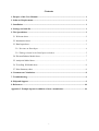
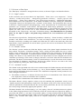
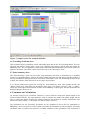
For the spreadsheet to function properly, macros need to be enabled in Excel. The security level in
“Tools
Macro
Security…” menu has to be set to “Medium (recommended)” or “Low” on the
Security Level tab (Figure 1) to enable the macros included in the workbook. On the “Trusted Sources”
tab, tick the box “Trust all installed add-ins and templates” and click OK. Please consult Excel’s
helpmenu if in doubt about security levels and protection.
The calculations completed in CS require an add-in, the “Analysis ToolPak”, to be activated in Excel.
In order to do this, go to “Tools
Add-Ins…” (a workbook must be open in Excel for this field to be
active), tick the box for “Analysis ToolPak” and click OK (Figure 1). The user may be asked to insert
the MS-Office installation CD at this point when the add-in was not initially installed on the computer
1
along with Excel. Please consult Excel’s help menu if you have problems with the installation of the
add-in.
IMPORTANT: If the “Analysis ToolPak” is not included or activated in Excel, or the user does
not set the security level on the “Tools” menu to those recommended above, CoronaScreen will
not run on your computer.
Figure 1: Setting the security level and installing add-ins to run macros in CoronaScreen
5. The Spreadsheet
To start CS, open the file by a double-click on the file-name or icon, or open it from Excel. The
workbook contains several worksheets to structure the data, input blocks and output sections. Some of
the sheets are hidden from view for clarity and become visible when needed. As with other Excel
workbooks, the tabs at the bottom of the window indicate the visible worksheets. Relevant sheets are
explained in the following sections.
The size of worksheets in this workbook is automatically adjusted according to the user’s screenresolution. If the adjustments are not accurate, this can be changed in the ‘Standard’ command bar by
changing the value in the percentage-field.
5.1 Welcome sheet
Upon opening the spreadsheet, a welcome worksheet becomes visible and allows the user to enter their
name, the name of the project and the date of the field survey. These fields will be shown in the header
of other worksheets throughout the workbook. The buttons in the right hand corner allows the user to go
directly to the “Introduction” or “Data Input” sheet.
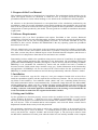
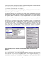
5.2 Introduction sheet
The “Introduction” sheet summarises the input parameters required for the three models used in CS
(Figure 2). It provides access to further information on the “Conceptual Model” used in each model for
the calculations completed in CS. Clicking the “Help” button opens the default web-browser and shows
an HTML-version of this document plus the user guides to the three models included in CS. Clicking
the “Go to Data Input” button takes the user to the main worksheet for data inputs used in CS. This can
also be done using the tab button at the base of the worksheets.
2
Figure 2. Introduction sheet
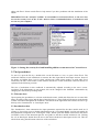
5.3 Data Input sheet
The “Data Input” worksheet is at the centre of the workbook (Figure 3). It is arranged in sections and
has several functions. These features are described in more detail below. Most functions, i.e. mainly
button-activated functions, are explained under the sections they can be found in. Dialogs linked to a
button-click are described separately in the second subchapter.
Figure 3. Data Input sheet
3
5.3.1 Sections on Data Input
The “Data Input” worksheet is arranged in three sections, as shown in Figure 3 and described below.
5.3.1.1 “Input” section
In this section the user can enter data in six input blocks -“Plume source term composition”,” Plume
chemistry: residual and products”, “Background groundwater chemistry”, “Aquifer properties and
hydrogeology”, “Plume source dimensions” and “Plume fringe parameters”. Compounds in the inputblock ‘Plume source term composition’ can be added or deleted as desired by clicking the “Add/Delete
Compounds” button (see description of the “Assistant” section below). The groundwater flow velocity
in the block “Aquifer properties and hydrogeology” can be entered directly or calculated from aquifer
parameters (see “Assistant” section below). The input block “Plume fringe parameters” is set up to
allow input of either the vertical thickness of the plume fringe or vertical transverse dispersivity of the
aquifer; the other value in each case is then calculated automatically. This dependency can be
decoupled on the “Dispersivity” tab under “Calculation settings”. Recommendations are provided
below for the input of alpha z and plume fringe thickness, dz, in CoronaScreen (see section
5.3.1.3).
The other three input blocks, “Background groundwater chemistry”, “Plume chemistry: residuals and
products” and “Plume source dimensions”, are static and simply require the user to enter the data
needed in each block, according to the model used. When the user clicks in the main body of the data
input blocks, a brief explanation for each of them is given in the text box at the bottom of the section
“Assistant” (see below).
5.3.1.2 “Results” section
The “Results” section contains the fields that display results of the plume length calculations for the
three models. The button “Calculation settings” shows a dialog box that enables the user to switch
models or parts of them on and off (see description of dialogs below). By clicking the “Calculate plume
length(s)” button, calculations of predicted plume length are performed according to the chosen
settings. This button is only enabled when data in the input blocks has been changed since the last
calculation (re-entering a value counts as change); otherwise it will show when the last calculation was
performed. The button “Print summary” leads to a sheet that keeps a record of the most recent scenario
(see description of “Summary” sheet below), which can be printed. The user can return to the “Data
Input” worksheet by clicking the “Back” button in this mode.
5.3.1.3 “Assistant” section
The column on the right hand side of the screen contains buttons for further functions and a description
box. On top of this column are three buttons (e.g. “Go to Electron Balance Model”) that lead to the
sheets showing information for the three models. The “Add/Delete compounds” button presents the user
with a dialog box that allows:
The addition of items to, or deletion of items from, the list of contaminants in the ‘Plume source
term’ input block, which are included in the CS database;
Addition of new contaminants to the database for future availability.
The button “Restore velocity equation” relates to the cell containing the groundwater velocity in the
‘Aquifer properties and hydrogeology’ input block. This button is only active if the user has entered a
value for groundwater velocity directly into the cell. By clicking this button, the user can revert back to
the velocity being calculated by applying the equation v = Ki/n.
The button denoted "Calc. dz from alpha_z" (or "Calc. alpha_z from dz") switches between two options
in the “Plume fringe parameters” block. When the cell for the vertical transverse dispersivity alpha_z is
greyed out and locked, i.e. user input is not possible, alpha_z is being calculated from the plume fringe
thickness, dz. After clicking the button, alpha_z becomes an input value and dz is being calculated. This
button is only available when alpha_z and dz are coupled (“Dispersivity” tab under “Calculation
settings”).
4
“Reset sheet to default values” will reset CS to a default dataset. This feature is only possible when
certain contaminants are included in the plume source term, but the program issues an alert if this is not
the case. The dialogs mentioned here are explained below.
5.3.2 Dialogs related to the Data Input worksheet
There are two dialog boxes which are accessed using the “Add/Delete Contaminants” button. These
dialogs are “Manage contaminants” and “Add new contaminant to database”.
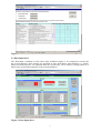
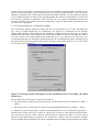
5.3.2.1 “Manage contaminants” dialog
This dialog box shows two lists (Figure 4). The right window lists the contaminants that are currently
being displayed in the “Plume source term composition” data input block and which will be included in
the calculations. When one of the items in this list is marked using the cursor, it can be deleted by
clicking the “Delete” button. Note that for technical reasons TOC and ammonium cannot be deleted
from the list of compounds included in the calculations. The concentration of these two components
should be set to “0” in the “Plume source term” data input block, when they are not required in the
calculations.
The left list shows all compounds that are currently contained in the CS database. A contaminant in this
list can be added to the right list (“Add” button) and included in the calculations, or its details can be
viewed (click “View” button). It is also possible to add a new contaminant to the list by clicking “Add
new…” and entering the relevant properties in the appropriate field on the pop-up dialog box. The latter
feature actually adds a new compound and its relevant properties to the workbook via the database,
whereas the other features are for the user’s convenience to keep irrelevant compounds out of view.
Figure 4. Dialog boxes for managing contaminants and adding contaminants to the
database
5.3.2.2 “Add new contaminant” to database dialog
On the “Add contaminant” dialog, a description of the input-fields is displayed in the text-box at the
bottom when the cursor is active in a field. Before adding a new compound to the database it is
recommended to view the details of existing contaminants to see an example showing the required
formats for the fields. The first four input fields are compulsory; the user will be alerted if data is
5
missing. The last two fields are optional. However, they should be completed where possible as they
provide a further description of the compound (in the case of the chemical formula) or are relevant for
additional calculations (the carbon balance in the Electron Balance Model). The only characters allowed
in the contaminant name are letters of the English alphabet, the underscore and numbers except for the
first character. Examples of input data needs and styles for new organic contaminants and electron
acceptors included in the “plume source term composition” using the “Add / Delete contaminants” tool
bar are shown in Appendix I.
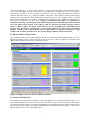
5.3.2.3 Dialog settings for “Calculations settings”
The “Calculations settings” dialog box allows the user to switch models “on” or “off” and change the
way values of aquifer dispersivity are calculated by CS (Figure 5). Calculations for the Electron
Balance Model and the Analytical Model can normally be enabled all the time since they are virtually
instantaneous and robust. The settings for the Travelling 1D Model as seen on the dialog box offer a
few more options. The default options will enable the user to get started for the first runs. It is
recommended that the user familiarises themself with the 1D Travelling Model before changing any of
the options (refer to the user guide for this model). Currently, alerts can be switched “on” or “off” in the
lower section of this dialog box.
Figure 5. Choosing models and options for the calculation (tab for Travelling 1D Model
shown here)
On the “Dispersivity” tab (Figure 5), the user can choose:
The ratio between vertical transverse dispersivity and horizontal transverse dispersivity, alpha_z /
alpha_y;
The ratio between vertical transverse dispersivity and longitudinal dispersivity, alpha_z / alpha_x;
Whether to couple dz and alpha z using the relationship built in to CS to estimate these parameters.
Default values of these ratios are 0.1 and 0.01, respectively, as these are often reported in the literature.
The user has the option to choose whether vertical transverse dispersivity, alpha_z, and the vertical
thickness of the plume fringe are coupled or not. If this box is checked, only one of the two variables
will be available and the remaining one will be calculated using an analytical approximation (use button
6
“Calc. dz from alpha_z” or “Calc. alpha_z from dz” to switch between alpha_z and dz). If this option is
not chosen, both alpha_z and dz are required as an input-value. Alternatively, the user may input a
value directly for alpha z in the relevant cell, when this is the only required parameter for a specific
model in this input section (e.g. Analytical Model). Note that a value of alpha z and the plume fringe
thickness, dz, are required for the Electron Balance Model, but that a value of alpha z only, is required
for the Analytical Model. In CS, alpha z is automatically calculated from the plume fringe thickness, dz,
when this is provided by the user. It is strongly recommended that alpha z is estimated for
individual sites using a measurement of the plume fringe thickness obtained from a MLS installed
across the plume fringe and the “Calc. alpha_z from dz” option in the model. Entering separate
values of alpha z and/or the plume fringe thickness, dz, by decoupling the relationship which
predicts these parameters (completed by accessing the “Dispersivity” tab in the “Calculation
settings” section of the model) should only be undertaken by experienced modellers, using
realistic values of these parameters for the scenario being evaluated with CoronaScreen.
5.4 Electron Balance Model sheet
This worksheet shows details and preliminary results of the Electron Balance Model (Figure 6). For a
detailed description of the various sections of this sheet, refer to the user guide for the model. The
“Back” button returns the user to the “Data Input” sheet.
Figure 6. Output screen for Electron Balance Model
5.5 Analytical Model sheet
This worksheet shows details, preliminary results and graphs for the Analytical Model (Figure 7). A
more detailed description of the various sections of this sheet is given in the user guide for this model.
The output includes profiles of predicted contaminant concentration along the plume centreline and
vertical electron donor-electron acceptor distributions across the plume fringe (Figure 7). The “Back”
button returns the user to the “Data Input” sheet.
7
Figure 7. Output screen for Analytical Model
5.6 Travelling 1D Model sheet
This worksheet shows preliminary results and further input data for the 1D Travelling Model. The user
can enter the number of time-steps n (not to be confused with porosity) and the time-step length for
PHREEQC here. For an explanation of this feature and background-information, please refer to the user
guide for the model. The “Back” button returns the user to the “Data Input” sheet.
5.7 Print Summary sheet
The “Print Summary” sheet lists the results, input parameters and time of calculation for a modelled
scenario in a printable format. It shows the plume lengths and other relevant data for the three models at
the top, in addition to the input blocks as seen on the “Data Input” sheet. The formatting has been set up
to allow the contents of this sheet to fit on two pages when printed.
It is a known problem that upon first viewing the “Print Summary” sheet after opening the file, the
“Plume source term” input block on the bottom of the page is not shown correctly. Click "<< Back",
and on the “Data Input” sheet and then click the “Print Summary” button again. The data should then be
displayed properly from now on.
6. Comment on Calculations
An iteration using Excel's ‘GoalSeek’ function is used to find the steady-state plume-length in the
Electron Balance Model. The same method is used to calculate the steady-state plume length and the
time to steady-state plume length in the Analytical Model. The iteration is virtually instantaneous and
known to be fairly robust, i.e. convergence is almost always achieved.
The calculations for the Travelling 1D Model are not completed in Excel, but are undertaken in
PHREEQC. Several steps in Excel are needed to facilitate the simulation run when using the Travelling
1D Model. Data is prepared and written to a hidden worksheet of the spreadsheet. This worksheet is
8
then saved as a plain data file (txt format) and used by PHREEQC as an input file. The user will be
alerted to this (unless this alert is switched off) and should make sure that any important data from
previous simulations is saved under a different name (the CS cannot save several solutions in one file).
Before the run is started, the user can either choose a name for the file to which selected PHREEQC
output data (which is required output for the Travelling 1D Model) is saved, or use the default name
(‘fringe.sel’). A dialog-box in Excel indicates that PHREEQC runs in the background. While the
program runs, the user can check on progress by activating the command window from the taskbar. It is
not recommended to use other applications while PHREEQC is running. The run can be interrupted at
any time from the displayed dialog in Excel ("Cancel" button). Once the run is completed, relevant
output data is read into Excel and processed to calculate the plume-length. Data for the Travelling 1D
Model is saved by default in a subdirectory of the main directory containing the CS (directory “odtrm”).
Users should note that since another application, PHREEQC via the DOS-window, is invoked for the
Travelling 1D Model, unforeseen complications cannot be ruled out due to the different ways
applications are treated on different computers.
7. Troubleshooting
The spreadsheet does not have an automated validation feature built in, i.e. input data is not tested for
consistency. The user has to ensure that only sensible parameter combinations are entered in the “Data
Input” worksheet. As an example, an organic carbon content (as fOC) or effective porosity (ne) larger
than 1.0 is not a realistic value, since both terms are fractions between 0 and 1.0. However, this kind of
inconsistency will not necessarily cause the calculations to fail or be directly visible in the results. Care
should therefore be taken when choosing sets of input parameters, which should be theoretically valid,
consistent with the scenario modelled, representative for the conceptual site model for the problem and
obtained from site-specific investigations, where possible.
Other falsely assigned input values may, however, not allow the iterations to converge, causing an error
message to be generated or cause Excel to display errors in cells (e.g. "#NAME?", "#REF?",
"#DIV/0"etc.). The cause in most of the cases is unrealistic values for input parameters, and the user is
advised to double-check the entered values for inconsistencies. Note that for the “Distance: source to
MLS well” input in the plume fringe parameters data block a value of “x” greater than one must always
be entered in this box to avoid “goal-seek error” or “#DIV/0!” messages occurring when the model is
run.
8. Help and Support
Every effort has been made to trap errors and return a meaningful error message that informs the user
about why and where the error occurred. However, due to the complexity of the spreadsheet and set-up
configuration for individual computers, no guarantee can be given that all errors are eliminated. The
cause in most cases will be inconsistent input data, which may be rectified easily by checking the error
message and double-checking the data set. However, if errors continue to occur, limited support for the
software and different models is available from the following sources in the Groundwater Protection
and Restoration Research Group at the University of Sheffield :
Technical problems and guidance
Assistance
Installation and use of CORONA Screen software
Arne Hüttmann ([email protected])
Electron Balance Model
Steven Thornton ([email protected])
Analytical Model
Marienne Gutierrez-Neri ([email protected])
Steven Thornton ([email protected])
Travelling 1D Model
Ryan Wilson ([email protected])
9
9. References
Parkhurst, D.L. and Appelo, C.A.J. (1999). User's guide to PHREEQC (Version 2)—A computer
program for speciation, batch-reaction, one-dimensional transport, and inverse geochemical
calculations: U.S. Geological Survey Water-Resources Investigations Report 99-4259, 310p.
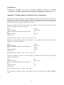
Appendix I. Example inputs for addition of new contaminants
The following examples illustrate how new contaminants (electron donors and electron acceptors) are
added to the CoronaScreen database using the “Manage Contaminants” tool bar in the “Add / Delete
contaminants” input option. The examples below are formatted in the style of information required by
the prompt boxes in the “Manage Contaminants” tool bar.
Example 1: Addition of methyl tertiary amyl ether (TAME) as a new organic contaminant (electron
donor) in the plume source term composition
Name:
Molecular weight:
Number of electron donated in redox half reaction:
Koc:
Chemical formula:
Carbon ratio:
TAME
102.18 g/mol
36
0
C6H14O
6
Redox half reaction: C6H14O + 11H2O → 6CO2 + 36H+ + 36eExample 2: Addition of methyl ether ketone (MEK) as a new organic contaminant (electron donor) in
the plume source term composition
Name:
Molecular weight:
Number of electron donated in redox half reaction:
Koc:
Chemical formula:
Carbon ratio:
MEK
72.1 g/mol
22
14 ml/g
C4H8O
4
Redox half reaction: C4H8O + 7H2O → 4CO2 + 22H+ + 22eExample 3: Addition of sulphate as a new inorganic contaminant (electron acceptor) in the plume
source term composition
Name:
Molecular weight:
Number of electron donated in redox half reaction:
Koc:
Chemical formula:
Carbon ratio:
SO4
96.06 g/mol
8
0
SO420
Redox half reaction: SO42- + 8e- +9H+ → HS- +4H2O
Note that inputs of electron acceptors in the plume source term composition are assigned a negative
value.
10