Download Aachen University of Applied Sciences, Campus Jülich Department

 Aachen University of Applied Sciences, Campus Jülich Department: Energy Technology Course: Electrical Engineering Bachelor Thesis Control and operation of an Imageplate‐Scanner for X‐ray diffraction Hangjian Cui 822331 Jülich, Oct. 2011 This bachelor thesis has been carried out at the Institute of Jülich Centre for Neutron
Science (JCNS) of the Research Center Jülich (FZ-Jülich).
This thesis was supervised by:
Prof. Dr. -Ing. Christoph Helsper
DI Klaus Bussmann
DI Peter Hiller
I certify that this work has been carried out and written up entirely by myself. No
literature references and resources other than those cited have been used.
Jülich, Oct.2011 ______________________
Acknowledgments First of all, I would like to show my deepest gratitude to Prof. Dr. –Ing. Christoph
Helsper for his constant encouragement and guidance. And I also want to thank Mr.
Klaus Bussmann, Mr. Peter Hiller and Dr. Ulrich Rücker for giving me this
opportunity to finish my bachelor thesis at institute of Jülich Centre for Neutron
Science (JCNS) of the Research Center Jülich (FZ-Jülich).
Further I would like to thank all professors of FH-Aachen for their help during my
study in Germany.
Finally, I would like to thank my parents and my friends for their deep love and
support.
Contents 1. Introduction of the system . . . . . . . . . . . . . . . . . . . . . . . . . . . . . . . . . . . . . . . . . . . 1
2. Scanning of neutron image plate . . . . . . . . . . . . . . . . . . . . . . . . . . . . . . . . . . . . . . . . 3
3. LabVIEW
3.1 Introduction of LabVIEW . . . . . . . . . . . . . . . . . . . . . . . . . . . . . . . . . . . . . 5
3.2 Basic use . . . . . . . . . . . . . . . . . . . . . . . . . . . . . . . . . . . . . . . . . . . . . . . . . . . 6
3.3 More functions . . . . . . . . . . . . . . . . . . . . . . . . . . . . . . . . . . . . . . . . . . . . . . 11
4. System Set-up
4.1 List of equipment . . . . . . . . . . . . . . . . . . . . . . . . . . . . . . . . . . . . . . . . . . . . 13
4.2 Optical scanner . . . . . . . . . . . . . . . . . . . . . . . . . . . . . . . . . . . . . . . . . . . . . . 15
4.3 Mini SAX. . . . . . . . . . . . . . . . . . . . . . . . . . . . . . . . . . . . . . . . . . . . . . . . . . 17
4.4 GSI Lumonics SC2000 Digital Scan Controller . . . . . . . . . . . . . . . . . . . . 18
4.5 Laser . . . . . . . . . . . . . . . . . . . . . . . . . . . . . . . . . . . . . . . . . . . . . . . . . . . . . . 20
4.6 Hooking up the system . . . . . . . . . . . . . . . . . . . . . . . . . . . . . . . . . . . . . . . . 21
4.7 Control of laser, lamp and photomultiplier tube . . . . . . . . . . . . . . . . . . . 25
4.7.1
DAQ card . . . . . . . . . . . . . . . . . . . . . . . . . . . . . . . . . . . . . . . . 25
4.7.2
Terminal block . . . . . . . . . . . . . . . . . . . . . . . . . . . . . . . . . . . . 27
4.7.3
Relays . . . . . . . . . . . . . . . . . . . . . . . . . . . . . . . . . . . . . . . . . . . 27
4.7.4
Circuit connection . . . . . . . . . . . . . . . . . . . . . . . . . . . . . . . . . . 28
5. Scan controller Support software
5.1 Introduction of the support program . . . . . . . . . . . . . . . . . . . . . . . . . . . . . 30
5.2 Command reference . . . . . . . . . . . . . . . . . . . . . . . . . . . . . . . . 33
5.3 Operation for scan controller . . . . . . . . . . . . . . . . . . . . . . . . . 34
5.4 Application . . . . . . . . . . . . . . . . . . . . . . . . . . . . . . . . . . . . . . . . 39
6. Own LabVIEW Interface
6.1 The whole program . . . . . . . . . . . . . . . . . . . . . . . . . . . . . . . . . . . . . . . . 40
6.2 Control of the movement of laser
6.2.1
SubVIs from GSI Lumonics . . . . . . . . . . . . . . . . . . . . . . . . . . 42
6.2.2
ComConfig set . . . . . . . . . . . . . . . . . . . . . . . . . . . . . . . . . . . . 43
6.2.3
Correction of the laser position . . . . . . . . . . . . . . . . . . . . . . . 44
6.3 Data process
6.3.1
Modes and files options . . . . . . . . . . . . . . . . . . . . . . . . . . . . . 44
6.3.2
2D-array into intensity graph . . . . . . . . . . . . . . . . . . . . . . . . 46
6.3.3
Simulation . . . . . . . . . . . . . . . . . . . . . . . . . . . . . . . . . . . . . . . . 47
6.3.4
Queue structure. . . . . . . . . . . . . . . . . . . . . . . . . . . . . . . . . . . . 48
6.3.5
Array . . . . . . . . . . . . . . . . . . . . . . . . . . . . . . . . . . . . . . . . . . . . 50
6.3.6
Event structure . . . . . . . . . . . . . . . . . . . . . . . . . . . . . . . . . . . . . 50
Conclusions . . . . . . . . . . . . . . . . . . . . . . . . . . . . . . . . . . . . . . . . . . . . . . . . . . . . . . . . . . 51
Appendix . . . . . . . . . . . . . . . . . . . . . . . . . . . . . . . . . . . . . . . . . . . . . . . . . . . . . . . . . . . . 52
References . . . . . . . . . . . . . . . . . . . . . . . . . . . . . . . . . . . . . . . . . . . . . . . . . . . . . . . . . . . 60
1. Introduction of the system The project is to scan a maximum 500mm × 500mm area neutron image plate by every
1mm grid with a Laser beam that is reflected by a moving magnet motor controlled
reflector system.
For each grid point there will be an analog value, that measured by photomultiplier tube
and then it is saved into the memory.
It should be also possible to read out the data and display into an intensity graph. The
system and the electronic components of the GSI-Lumonics Group must work with the
Class-3B-Laser to set up an experiment.
The LabVIEW, which is used in the project, is from the National Instrument Company.
Practical work procedure:
• Learn LabVIEW to be familiar with using and building programs.
• Set-up the hardware system with the electronic components of the
GSI-Lumonics Group and connect with the host computer with LabVIEW.
• Set-up another circuit to control laser, lamp and photomultiplier tube with
DAQ-Card, terminal block and relay.
• Install the program CLI.exe (Command Line Interface) from the CD of GSI
Group, and be familiar with using commands to control the system.
• Use LabVIEW to build up an own program to control the system also laser,
lamp and photomultiplier tube with the SubVIs that are in the CD.
• Also write one part program that can acquire and proceed the data that will be
displayed into an intensity graph.
1
T HE ORIGINAL PROJECT DESCRIPTION : Steuerung und Inbetriebnahme eines Imageplate­Scanners für Röntgendiffrakometrie Als 2-dimensionalen Detektor für eines unserer Röntgendiffraktometer möchten wir
eine Röntgen-Imageplate mit einem Scanner benutzen, der programmierbar vor Ort die
Imageplate ausliest und die Daten über ein Computersystem zur Verfügung stellt. Eine
Röntgen-Imageplate ist heutzutage kommerziell erhältlich und wird in der
medizinischen Röntgentechnik serienmäßig verwandet. Allerdings wird sie dort im
allgemeinen nicht am Ort der Belichtung ausgelesen, sondern ausserhalb des
Röntgenstrahls in einem externen Scanner. Wir hingegen möchten Sie am Ort der
Belichtung auslesen können, um ohne Justageungenauigkeiten mehrfache Experimente
durchführen zu können.
Wir haben einen Aufbau fertiggestellt (s.Abbildung), in dem mittels eines Lasers und
zwei Spiegelgalvanometer die Platte systematisch gescannt werden kann. Die
Fluoreszenzstrahlung der belichten Imageplate wird dann mit einem Photomultiplier
detektiert und über einen AD-Wandler in den Computer eingelesen. Die aufbereiteten
Messwerte sollen gespeichert und visualisiert werden.
Die Steuerungs- und Projektierungssoftware ist LabVIEW von National Instruments.
Die Arbeit setzt auf ein bestehendes Softwaregerüst auf. Das Projekt umfasst den
Aufbau, die Inbetriebnahme und abschließenden Test der Hard- und Software unter
Messbedingungen.
Die Arbeit wird betreut von Herrn DI Klaus Bussmann (Elektrotechnik, Laborleiter des
Elektroniklabors) und Herrn DI Peter Hiller (Physikalische Technik, Laborleiter des
Röntgenlabors).
2
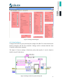
2. Scanning of neutron image plate Neutron image plate (NIP) has found widespread application as neutron detectors for
single-crystal and powder diffraction, small-angle scattering and tomography. After
neutron exposure, the image plate can be read out by scanning with a laser (see figure
2.1). Commercially available NIPs consist of a powder mixture of BaFBr : Eu2+ and
Gd2O3 dispersed in a polymer matrix and supported by a flexible polymer sheet. Since
BaFBr : Eu2+ is an excellent x-ray storage phosphor, these NIPs are particularly
sensitive to γ –radiation which is always present as a background radiation in neutron
experiments. In this work we present results on NIPs consisting of KCl : Eu2+ and LiF
that were fabricated into ceramic image plates in which the alkali halides act as a
self-supporting matrix without the necessity for using a polymeric binder. An
advantage of this type of NIP is the significantly reduced γ -sensitivity. However, the
much lower neutron absorption cross section of LiF compared with Gd2O3 demands a
thicker image plate for obtaining comparable neutron absorption. The greater thickness
of the NIP inevitably leads to a loss in spatial resolution of the image plate. However,
this reduction in resolution can be restricted by a novel image plate concept in which a
ceramic structure with square cells (referred to as a ‘honeycomb’) is embedded in the
NIP, resulting in a pixelated image plate. In such a NIP the read-out light is confined to
the particular illuminated pixel, decoupling the spatial resolution from the optical
properties of the image plate material and morphology. In this work, a comparison of
experimentally determined and simulated spatial resolutions of pixelated and
unstructured image plates for a fixed read-out laser intensity is presented, as well as
simulations of the properties of these NIPs at higher laser powers.
-<Pixelated neutron image plates> Certain materials, notably BaFBr:Eu+2, have energy levels below the conduction band
which can be populated when x-rays de-excite in the material. These levels cannot
de-excite to lower levels and are sufficiently below the conduction band that thermal
excitation to the conduction band is very unlikely. Photoexcitation, e.g., by a red laser,
into the conduction band then allow de-excitation with the emission of a blue photon.
This is photostimulated luminescence. A phototube covered with a filter to only pass
blue photons then can sense the magnitude of photostimulated luminescence without
sensing scattered red laser photons. An intense flood of light is used to totally
photostimulate the plate, thereby erasing it.
3
Figure 2.1 Principle of neutron image plate exposure and evaluation
Also known as an image plate, a photostimulable phosphor (PSP) plate can be used
record a two-dimensional image of the intensity short-wavelength (typically, X-ray)
electromagnetic radiation. The device to read such a plate is known as a
phosphorimager (occasionally abbreviated to phosphoimager, perhaps reflecting its
common application in molecular biology of detecting radiolabeled phosphorylated
proteins and nucleic acids).
4
3. LabVIEW 3.1 Introduction of LabVIEW What is NI LabVIEW ? LabVIEW is a graphical programming environment used by millions of engineers and
scientists to develop sophisticated measurement, test, and control systems using
intuitive graphical icons and wires that resemble a flowchart. It offers unrivaled
integration with thousands of hardware devices and provides hundreds of built-in
libraries for advanced analysis and data visualization – all for creating virtual
instrumentation. The LabVIEW platform is scalable across multiple targets and OSs,
and, since its introduction in 1986, it has become an industry leader.
-http://www.ni.com/labview/whatis/
LabVIEW is a powerful and flexible development software and designed specifically
for the needs of scientists and engineers. It uses the graphical programming language G
to create programs which called virtual instruments (VIs) in the block diagram. The
user interacts with the program through the front panel. LabVIEW has many build-in
functions to facilitate the programming process.
Block diagram: Pictorial representation of a program or algorithm. In G language, the
block diagram, which consists of executable icons, called nodes, and wires that carry
data between the nodes, is the source code for the VI.
Front panel: The interactive interface of a VI. Modeled from the front panel of
physical instruments, it is composed of switches, slides, meters, graphs, charts, gauges,
LEDs, and other controls and indicators.
5
3.2 Basic use Example1: for loop and while loop For loop: Calculate 5 times, i starts from 0 not 1, so the last time i=4, the indicator
display the result i+1=5.
While loop: Keep calculating till press the stop button, if the i=2332859 at that moment,
the indicator display the result i+1=2332860.
For loop in other programming language: Java for (int i=0; i<10; i++){
System.out.println("The value of 'i' is " + i );
}
6
C++ int i;
for (i=0; i<10; i++){
cout << "The value of 'i' is " << i << endl;
}
While loop in other programming language: Java int i = 0;
while (i < 10){
System.out.println("The value of 'i' is " + i);
i++;
}
C++ int i = 0;
while (i < 10){
cout << "The value of 'i' is " << i << endl;
i++;
}him
Example2: case structure In case structure, we use normally boolean, which has TRUE and FALSE value. When
the boolean is true, the program runs the process only in true structure (Figure 3.1).
When the boolean is false, the program runs the process only in false structure (Figure
3.2). It’s easy to make a program with case structure and it’s very useful.
7
Figure 3.1 True case Figure 3.2 False case
Example3: data acquisition (DAQ) Data acquisition is the process of sampling signals that measure real world physical
conditions and converting the resulting samples into digital numeric values that can be
manipulated by a computer. Data acquisition systems (abbreviated with the acronym
DAS or DAQ) typically convert analog waveforms into digital values for processing.
The components of data acquisition systems include (see figure 3.3):
• Sensors that convert physical parameters to electrical signals.
8
• Signal conditioning circuitry to convert sensor signals into a form that can be
converted to digital values.
• Analog-to-digital converters, which convert conditioned sensor signals to
digital values.
Data acquisition applications are controlled by software programs developed using
various general purpose programming languages such as BASIC, C, Java, MATLAB
and LabVIEW. Figure 3.3 Data acquisition system First of all, we must install DAQ-Driver, that can be downloaded from NI website.
When we place the DAQ Assistant Express VI on the block diagram, the DAQ
Assistant automatically appears. And then we can choose acquire or generate of analog
or digital signals. The DAQ Assistant is a graphical interface that we can use to
configure measurement tasks and channels. We use acquire analog signal to get voltage
value.
Figure 3.4 DAQ Assistant 9
Figure 3.5 Voltage indicator The LabVIEW graphical dataflow language and block diagram approach naturally
represent the flow of your data and intuitively map user interface controls to your data,
so you can easily view and modify your data or control inputs.
For experienced programmers, LabVIEW delivers the performance, flexibility, and
compatibility of a traditional programming language such as C or BASIC. In fact, the
full-featured LabVIEW programming language has the same constructs that traditional
languages have -- variables, data types, looping, and sequencing structures as well as
error handling.
10
3.3 More functions · Faster Programming Graphical Programming Program with drag-and-drop, graphical function blocks instead of writing lines of text.
Dataflow Representation Easily develop, maintain and understand code with an intuitive flowchart
representation.
· Hardware Integration with LabVIEW I/O and Communication Connect to any instrument or sensor with built-in libraries and thousands of instrument
drivers.
Plug‐and‐Play Hardware Seamlessly integrate NI plug-and-play devices for USB, PCI, PXI, Wi-Fi, Ethernet,
GPIB, and more.
· Advanced Built­In Analysis and Signal Processing Built‐In Analysis Access thousands of engineering-specific functions such as frequency analysis, curve
fitting, and more.
Inline Signal Processing Interact with measurements and perform inline analysis in real time on acquired
signals.
· Data Display and User Interfaces Built‐In Controls Interact with data using hundreds of drag-and-drop controls, graphs, and 3D
visualization tools.
Custom Controls Easily customize the position, size, and color of built-in controls or create your own in
seconds.
11
· Multiple Targets and OSs Desktop and Real‐Time OSs Develop and reuse code on Windows, Mac, Linux, and real-time OSs such as
VxWorks.
FPGAs and Microprocessors Target various embedded architectures, including ARM microcontrollers and FPGAs,
with the same graphical approach.
· Multiple Programming Approaches Code Reuse Integrate text-based code and DLLs or easily incorporate native and third-party .m
files.
Various Design Patterns Incorporate additional models of computation such as dynamic simulation diagrams
and statecharts.
· Multicore Programming Automatic Multithreading Handle large data sets and complex algorithms faster because LabVIEW inherently
runs on multiple threads.
Execution Highlighting Easily optimize code for parallel execution using built-in debugging and visualization
tools.
· Data Storage and Reporting File I/O Designed for Engineering Data Focus on your data and not converting formats with built-in support for a wide variety
of file types.
Flexible Reporting Tools Share your results by generating reports from your acquired data.
12
4. System Set­up (Hardware Description) 4.1 List of equipment The following is a list of the equipment used. A detailed description of the most
important components can be found in the next parts.
- Power Supply (±15V)
Typ: MADS 15.1.6
A.-Nr.: 171-602-00.02
U in: 115/*230V +10/-15% 50-400Hz
I in Max.: 0.8/0.4A
KNIEL System-Electronic GmbH D-76187 Karlsruhe/Germany
IS: 16880159
- SC2000 Scan Controller Board
GSI Lumonics
IS: 03071011
- X and Y Optical Scanners
GSI Lumonics
VM-500
011-3040106
IS: 03070903/03070904
- 2 MiniSAX (Miniature Single Axis)
GSI Lumonics
Billerica, MA 01821 USA
Model Number: 002-3005051
IS: 03070905/03070906
- Laser beam
●Laser radiation avoid exposure to beam class 3B laser product
Iop: 1450mA
Power: ≥75mW
A-A1728-0109
Laser protect glasses
Laser 2000 GmbH- TÜV ISO 9001 zert.
Laserschutzbrille Modell 426
13
BOL-40-426
Wareneingang: 2210921
2203002
●Laser radiation class 2 (for safty)
- 1 Power Supply cable
- 2 Startup SAX Interface Cables, part# 712-74217
- 2 Enable Interlock SAX Interface Cables
- 2 Dual Axis Digital Servo Interface Cables
- 1 RS-232 Computer Interface Cable, part# 712-74214
- 1 Sync/Cal Ribbon Cable
- Host Computer
- NI DAQ-Card 6024E
- Terminal Block CB-68LP
- Relays
- CD of GSI Lumonics CD-ROM SC2000 CLI 2.1
- LabVIEW 2009 and DAQ driver
14
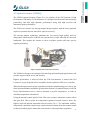
4.2 Optical Scanner (VM500) The VM500 Optical Scanner (Figure 4.1) is a member of the GSI Lumonics’ High
Performance VM family of Galvanometers. It’s designed for advanced beam and image
positioning, and offer high dynamic performance along with high accuracy and
instrument grade performance.
The VM Series scanners use moving-magnet design together with the newly patented
capacitive position detector that offers superior accuracy.
The moving magnet technology maintains the low inertia, high rigidity and low
temperature characteristics of the M series predecessors, while allowing for increased
bandwidth. This enables the scanner to move at higher speeds with more precise
angular positioning.
Figure 4.1 Optical scanner and control electronics The VM Series Scanners are optimized for both large and small signal applications, and
provide improved drift, noise, and linearity.
Highest performance is achieved when the VM Galvanometer is mated with GSI
Lumonics’ newly designed mirror assemblies and an optimized GSI servo controller.
When the thermal control option is purchased with the complimenting servo driver, the
built-in thermal blanket around the position detector that is a standard feature of all VM
Series Galvanometers can be used to maintain a specific temperature, in order to
eliminate temperature-related drift.
Using the thermal control option of the VM series scanners minimizes scanner offset
and gain drift. The set point for temperature-regulated scanners must be above the
highest expected ambient temperature but not above 50º C. For maximum stability,
temperature controlled scanners may require thermal isolation from the scanner mount
so that heat sinking by the mount does not interfere with temperature regulation.
15
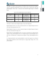
Standard Mirrors (clear aperture)
Maximum Scan Angle
VM500
4mm
±30o Optical
5mm
±25o Optical
6mm
±20o Optical
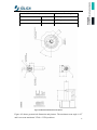
Figure 4.2 Geometrical dimension and pinout Figure 4.2 shows geometrical dimension and pinouts. The maximum scan angle is 30o
and it can scan maximum 32768 x 32768 positions.
16
4.3 Mini SAX The MiniSAX (Miniature Single AXis) servo controller (Figure 4.3) is one of GSI
Lumonics’ most recent developments in galvanometric servo control technology. By
taking advantage of the newest surface mount components, the MiniSAX provides
full-function scan electronics at a size and cost less than many stripped down servo
amplifiers. Advanced servo filtering techniques together with a low-coupling design
provide extended bandwidths and improved response times. The MiniSAX was
engineered with system designers in mind, incorporating a simple yet comprehensive
and flexible interface structure. For the first time, laser system manufactures can
purchase a truly high performance, cost effective galvanometer servo controller that
allows convenient, “in-head” packaging.
The MiniSAX uses a modular design, providing the ability to readily configure the
driver for specific applications. An optional filter module is available in a variety of
adjustable notch frequency ranges. The frequency response of this module can be
optimized to handle a variety of customer-supplied loads. A thermal control module is
available to support GSIL’s thermally regulated scanners, allowing use of the
industry’s lowest drift galvanometers.
The MiniSAX product line includes a variety of accessories that ease the integration
into your manufacturing process. The MiniSAX mounting bracket provides convenient
mounting surfaces and mates with either of two optional heatsinks. A test interface
board allows easy access to a variety of important test points. Mating connectors and
inexpensive assembly tools are available directly from GSI Lumonics. The MiniSAX
Startup Kit is recommended for first time users and includes many of these valuable
accessories.
Figure 4.3 Mini SAX 17
Figure 4.4 Mini SAX connections
4.4 GSI Lumonics SC2000 Digital Scan Controller The SC2000 Scan Controller (Figure 4.5) is designed to provide fast, accurate,
user-friendly control over GSI Lumonics’ MiniSAX and Dual Axis Digital servo
amplifiers and associated peripherals. Using either the provided GSI Lumonics
Command line interface software, or similar user-designed software, the controller can
be programmed to operate in conjunction with a host computer or in a stand-alone
configuration. The stand-alone configuration allows the user to run a series of programs,
from non-volatile memory upon system power up, as well as trigger program execution
using control input and output signals. Interfacing with a host computer, on the other
hand, allows the user to choose a mode of operation, between the controller and the host,
ranging from totally autonomous to tightly coupled.
Figure 4.5 SC2000 digital scan controller
18
The Scan Controller interfaces directly to the position command, position feedback,
and binary communications of the servo amplifiers. This allows for full position control
of the system and control of the enable/status interlock between the SC2000 and driver
board. Likewise, this interface allows the user to monitor position feedback from the
galvo, as well as read calibration information digitally via the host computer.
In addition to controlling the servos, the Scan Controller has hooks to aid in the
interface and control of other peripherals typically associated with scanning systems.
These include sync inputs and outputs, a pixel clock system, a calibration/data capture
system, and other functionality available to volume OEM system designers.
Figure 4.6 Pinout of scan controller 19
4.5 Laser In this project lasers of class 2 and 3B have been used. The definition of these laser
classes are given below:
Class 2: Low risk to eyes. No risk to skin
Class 2 laser products are defined as those emitting visible light for which the natural
aversion response to bright light (including the blink reflex) prevents retinal injury,
including direct viewing of the laser beam with optics that could concentrate the laser
output into the eye. These lasers do, however, present a dazzle hazard.
Lasers that were Class 2 under the previous version of 60825-1 remain Class 2 under
the new scheme.
Warning label: DO NOT STARE INTO BEAM
Only use Class 2 for safety during the experiments in room.
Class 3B: Medium risk to eyes. Low risk to skin
Class 3B laser products are defined as those for which direct exposure of the eye is
hazardous, even taking aversion responses into account, but scattered laser light is
usually safe. The higher power Class 3B lasers are also a skin hazard, but the natural
aversion response to localised heating generally prevents a skin burn. Lasers that were
Class 3B under the previous version of 60825-1 but which operate at a wavelength in
the range 0.3025 to 4 µm and have output beams that are either high divergence or large
diameter may qualify.
Warning label: AVOID EXPOSURE TO THE BEAM
In the project two different lasers are used. Class 2 laser is used to test the position of
laser and class 3B laser is used to scan the image plate. Because class 2 laser is safe and
it is weak to exposure photons.
20
4.6 Hooking up the system The components of the system are connected according to the user manual.
Figure 4.7 System connection Step 1 Before you begin: • Be sure power supply is turned off.
• Be sure make all connections firmly. Loose connections may cause
communications and/or performance problems.
• Be sure wearing a properly grounded wrist strap or heel strap. Components
on the SC2000 Controller board are highly sensitive to electrostatic
discharge.
Step 2 Connecting the Power Supply: • Using the provided power cable, connect the stripped leads to the power
supply terminals as labeled:
+15V to the positive supply terminal
COM to the common terminal
-15V to the negative supply terminal
• Plug the power cable’s Molex connector into the pwr connector, J2, on the
SC2000 controller board.
21
Step 3 Connecting the servo Interface Cables: For the MiniSAX servo amplifier:
• Using a Startup SAX Interface Cable (part numbered 712-74217), connect
the X axis interface (J3) on the SC2000 to the X axis MiniSAX command
interface (J2 on the SAX board).
• Use the remaining Startup Interface Cable to connect the Y Axis interface (J8)
on the SC2000 to the Y axis MiniSAX command interface (J2 on the SAX
Board).
• Connect the X axis controller command interface, J3 on the SC2000, to the X
axis servo command interface (J3 on the underside of the Digital Servo).
• Use the remaining command cable to connect the Y axis command interface,
J8 on the SC2000 to the Y axis servo command interface (J4 on the
underside of the of the Digital Servo).
Step 4 Connecting the Host Computer: • Connect the provided Computer Interface Cable (part number 712-74214) to
an available serial port on your host computer. Remember which serial port
you use since you will need to know which port to address when
communicating with the controller board. Connect the other end of the
cable to the Serial Interface connector (J1) on the controller board.
22
Step 5 Sync/Cal Connections (Optional): The Sync/Cal connector provides access to the synchronization /calibration I/O as well
as the pixel clock output of the Scan Controller. Figure 3 shows a system using one of
the (open drain) sync outputs and the auxiliary +5V output to power and control a diode
laser module.
For further information on the Sync/Cal and pixel clock features of the scan controller,
read the GSI Lumonics Scan Controller Users Manual.
For controlling a low power laser diode module:
• Connect laser diode (+) output to +5V output (J2, pin 1) of the Scan
Controller.
• Connect laser diode (-) output to sync gnd (J4, pin 5) on the Scan Controller.
• Connect laser diode modulation control output to sync 1 (J4, pin 1) on the
Scan Controller.
Note: User must supply a 4.7k pull up resistor between the +5V and Sync 1.
There are other ways to interface to a laser. For example connect the + lead to +5V and
the – lead to the sync pin. This would be good enough for users who don’t need high
performance switching.
Warning: Check the manufacturer’s voltage and current specifications before hooking
up a laser diode or any other peripheral. The open drain outputs on the Scan Controller
(sync 1–4) are specified to sink up to 100mA continuous, and withstand peaks up to 40
V. These output must be clamped if inductive loads are to be driven (i.e. a small relay).
Otherwise, the voltage transient generated at turn-off can destroy the sync output
transistors.
Step 6 Software Installation: The GSI Lumonics Command Line Interface software discussed in the manual can be
found on the provided CD-ROM. Read the ReadMe.txt file for the latest information
and changes.
• To install the software run ‘<CDROM> :\install\disc 1\setup.exe’. The setup
program will create a default installation directory (typically C:\GSI),
install the application and support files and peripheral tools, create a
program group and add an item in the Windows start menu.
• If using a Servo/Galvo pair, connect galvo to driver board.
23
Step 7 Final Setup: • If using a Servo/Galvo pair, connect galvo to driver board.
• Double check all connections to make sure they are correct and secure.
Figure 4.8 Detailed system connection
24
4.7 Control of laser, lamp and photomultiplier tube The other circuit controls other hardware, such as laser, lamp and photomultiplier tube
that are controlled by DAQ-Card, terminal block and relays.
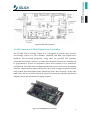
4.7.1 DAQ­Card 6024E Figure 4.9 DAQ‐Card 6024E The National Instruments PCI-6024E shown in figure is a low-cost data acquisition
board that uses E Series technology to deliver high-performance, reliable data
acquisition capabilities in a wide range of applications. You get up to 200 kS/s
sampling and 12-bit resolution on 16 single-ended analog inputs. Depending on your
type of hard drive, the NI PCI-6024E can stream to disk at rates up to 200 kS/s.
With this we can get data and signals or produce signals to terminal block. Also it can
measure real world physical conditions and converting the resulting samples into
digital numeric values that can be manipulated by a computer.
25
Figure 4.10 NI 6024E Pinout
26
4.7.2 Terminal block CB­68LP Figure 4.11 Terminal block CB‐68LP The NI CB-68LP is a low-cost termination accessory with 68 screw terminals for easy
connection of field I/O signals to 68-pin data acquisition products. It includes one
68-pin male SCSI connector for direct connection to 68-pin cables. The connector
blocks feature standoff feet for use on a desktop or mounted in a custom panel. The
CB-68LP has a vertical-mounted 68-pin connector.
It is connected with DAQ-Card and these 68 pinouts are the exactly same as DAQ-Card
pinouts above. It is one “magnification” of DAQ-Card pinouts.
For example, we use Digital Output to control laser, lamp and photomultiplier tube.
And we use Counter to measure the number of pulse in the limited time.
4.7.3 Relays A relay is an electrically operated switch. Many relays use an electromagnet to operate
a switching mechanism mechanically, but other operating principles are also used.
Relays are used where it is necessary to control a circuit by a low-power signal (with
complete electrical isolation between control and controlled circuits), or where several
circuits must be controlled by one signal. The first relays were used in long distance
telegraph circuits, repeating the signal coming in from one circuit and re-transmitting it
27
to another. Relays were used extensively in telephone exchanges and early computers
to perform logical operations.
We connect relays to terminal block which provides about 5V for pins when they are
open. The relays for laser and lamp are connected to the Digital Outputs of the terminal.
We give a True signal to Digital Outputs by LabVIEW to open these pins. They provide
5V and so relays are closed and outputs of relays are connected. So the laser and lamp
are open. For photomultiplier tube we use external input instead of use internal input
(220V). It works when we supply only 5V to the external input. So we use relay in the
opposite way. When we give a True signal to Digital Output of the terminal block, it
would be closed and output of relay is connected. It means no voltage at output of relay.
So photomultiplier tube is off. When we give a False signal to Digital Output of the
terminal block, it would be opened and output of relay is disconnected. It means there is
5V at output of relay. So photomultiplier tube is on.
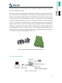
Figure 4.12 Relays (left from ABB, right from PhoenixContact)
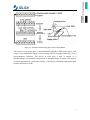
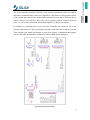
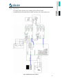
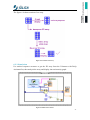
4.7.4 Circuit connection Figure 4.13 Circuit connection
28
The figure 4.13 shows circuit connection. The DAQ-Card is inserted in the computer.
And it is connected terminal block. There are three relays to control laser, lamp and
photomultiplier. Each relay is connected with different digital output of terminal
block.
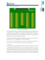
Table 4.1 Status of digital outputs, relays and components
Digital output for
Laser
Lamp
Photomultiplier
Status of output
on
off
on
off
on
off
Relay
connected
disconnected
connected
disconnected
connected
disconnected
Component
on
off
on
off
on
off
The table 4.1 shows status of digital outputs, relays and components.
Digital Output for laser is on, relay is connected, laser is on. Digital Output for laser is
off, relay is disconnected, laser is off.
Digital Output for lamp is on, relay is connected, lamp is on. Digital Output for lamp is
off, relay is disconnected, lamp is off.
Digital Output for photomultiplier tube is on, relay is connected, no voltage between
outputs of relay, photomultiplier tube is off. Digital Output for photomultiplier tube is
off, relay is disconnected, 5 voltage between outputs of relay, photomultiplier tube is
on.
It is important that the relay for photomultiplier is used in the opposite way. Because
high voltage transformer needs external power to supply high voltage (1kV) to the
photomultiplier.
29
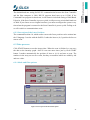
5. Scan controller support software 5.1 Introduction of the Support Program The Command Line Interface software written in LabVIEW allows users to
communicate with the Scan Controller quickly and easily. It is intended primarily as an
environment for designing and programming stand-alone applications, and for system
evaluation. Using Command Line Interface software during system evaluation
provides a user-friendly learning environment in which functional capabilities of the
Scan Controller can be understood and applied. Once the functionality and limitations
of the Scan Controller are understood, designing host-based, real-time system
programs becomes much easier. While pieces of the provided code can be utilized in
host-based, real-time systems, that is not its primary intent.
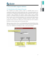
When you start to run the CLI.exe, it will automatically raise the Serial Port selector
sub-window asking you to set the serial port device for Scan Controller communication.
Choose one COM that was used and press ‘Done’ to enter your serial port.
30
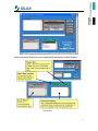
Here is the main Functions of the Command Line Interface Main Window:
31
32
5.2 Command Reference The Command Line Interface (CLI) and the Motion Assembler Component (MAC)
incorporate assemblers that translate English language program commands into the
binary language of the SC2000. Each command in defined in the assembly language
context and then in the binary context, but note that the SC2000 will only accept
commands uploaded in the binary format.
In order to exert the program efficiently we need to be familiar with the Commands of
the program especially these in boldfaced that will be used in the project.
For more commands see appendix.
Explanation of operational modes Overview: There are various modes of operation that overlap or are mutually exclusive
depending upon those compared.
Raster Mode: A fundamental operating mode for either programs or immediate
instructions in which all motion commands are directed to a specified axis.
Vector Mode: A fundamental operating mode for either programs or immediate
instructions where motion commands are simultaneously directed to the both X and Y
axis.
Program Instruction Mode: When a program is running the operational context of the
instructions of the program will be Program Instruction Mode. In contrast, query
commands and the system configuration commands cannot be executed from a
program, i.e. they are not valid in Program Instruction Mode.
Immediate Instruction mode: This is the idle mode of the Scan Controller, when a
program is not running. Typically, every command can be executed from this mode
except those that deal exclusively with the operation of programs, i.e. Repeat, Nrepeat,
End, and ExecuteSerialNumber.
Dual Single Axis: This mode is only available when the ExecuteRasterPgm command
is executed. This mode is characterized by two raster programs running concurrently,
one on each axis.
Concurrent Instruction mode: This mode comes about when a program is running
and you try to enter a command over the communications interface. Typically,
commands valid for this mode are the query commands, AbortPgm and ExitPGM.
33
5.3 Operation for Scan controller To be familiar with the software commands, several basic operations have been
performed by using the command line interface (CLI).
1.
Use the command ‘?status’ to make sure there is no errors with the system.
‘Success’ will be shown in the Response window.
2.
Fix the laser beam in a proper location, check the position and the direction of the
scanning point.
34
3.
To correct the position and the direction of the moving point, we need to know how
many degrees should be turned and how many steps should be changed to the 0
point. Then use the ‘rotate calculator’ to get the commands. After these commands
entered into the command line the coordinate of the laser been will just changed to
fit the image plate.
As the image plate in our experiment is oriented an angle of 45o, the relation
between the X and Y coordinate and the angle positions of the mirrors depend on
the coordinates. The necessary corrections can be obtained using the “rotate
calculation”.
In fact the orbit of scan is a curve because of degrees between mirrors and image
plate. It is too complicate to calculate correct position for each point to make
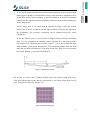
linear orbit. So we make the curve to line (Figure 5.1). It is easy to calculate how
much distance y-axis mirror should move. The maximum distance between ideal
orbit and real orbit d divided by l is the slope of the line. With it we can calculate
how much distance y-axis mirror should move.
Figure 5.1 simplify of scan orbit
The project is to scan a max. 500mm×500mm large area neutron image plate every
1mm grid with the laser beam. But for experiment we use 10cm×10cm large area by
every 1cm grid as a first step (Figure 5.2).
Figure 5.2 Ideal scanning orbit
35
The following program performs this scan.
CreatePGM 1 'a'
Setsync 1
wait 100
slewxy 500 0 1
wait 100
slewxy 1000 0 1
wait 100
……
wait 100
slewxy 4500 0 1
……
slewxy 4000 -5000 1
wait 100
slewxy 4500 -5000 1
wait 100
slewxy 5000 -5000 1
wait 100
positionxy 0 0
wait 100
repeat
end
//create a task
//laser is on (1 means laser is open)
//scan to position (500,0) with open laser
//wait 100ms
//go back to default 0,0 position
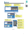
• Save program as a .txt file in the desired directory. Running the Vector Mode Program
• Click on the [File Ops] button in the Main Program Window of the Command Line
Interface.
36
• In the Load Subpanel, select ‘Source Code’ as the Program Source and ‘Scan
Controller’ as the Program Destination. Press Done.
37
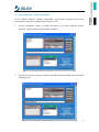
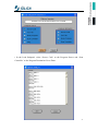
• In the File Dialog box, select the saved .txt program. Press ‘OK’. This brings up the
Upload Configuration Sub-window shown below. This window provides a type of
stream editor where it is possible to change commands, add or remove lines or change
the name of a program without changing the original source file.
• To assemble and upload the program click (Done). The program is then automatically
assembled and uploaded into the Scan Controller. If the assembler detects an
improperly formatted command in the program, assembly is halted and an error
message is returned to the Main Program Window. If this occurs, correct the error in the
text file and then reload the program. While the program is being assembled and
uploaded, the Command Line ‘Ready’ indicator switches from green to red and
indicates that the command line is Busy. Assembly and Uploading information is
provided in the Response Window.
• Once the upload is complete, and the Command Line ‘Ready’ Indicator turns green,
execute the program. In the Command Line Window, enter: Executepgm ‘a’
The Scan Controller will then begin running the uploaded program and sending
commands to the servo drivers.
If nothing happens after entering the Executepgm command:
• Check Scan Controller servo Interface connections.
• Be sure power is applied to servo boards and that galvos are properly
connected.
• Execute a ?Status Query to check for possible communications failure.
• Make sure that 'a' was typed in quotes
To Stop Program:
ExitPgm acts as a soft stop and will run through the remainder of the program before
stopping.
AbortPgm terminates the program immediately.
38
5.4 Application Command Line Interface also has many other functions, such as scan a circle track
(Figure 5.3) or even Letters in different fonts. Because the Optical Scanner moves quite
fast so it seems to be coherent lines.
Figure 5.3 Example of other function 39
6. Own LabVIEW Interface 6.1 The whole program This program is based on queue structure which is called Producer/Consumer Design
Pattern. Use this template to build a producer/consumer design pattern with events to
produce queue items. Use this design pattern instead of the User Interface Event
Handler pattern for user interfaces when you want to execute code asynchronously in
response to an event without slowing the user interface responsiveness. It is made up of
several parts such as data acquiring, 2D-Array, intensity graph processing and so on.
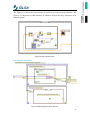
The figure 6.1 shows front panel of the interface. It is composed of switches, graphs,
LEDs, and other controls and indicators. The detailed functions will be found in next
parts.
Figure 6.1 Front panel of the interface 40
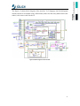
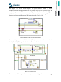
The figure 6.2 shows block diagram of the interface. In G language, the block diagram,
which consists of executable icons, called nodes, and wires that carry data between the
nodes, is the source code for the VI.
Figure 6.2 Block diagram of the interface 41
6.2 Control of the movement of Laser 6.2.1 SubVIs from GSI Lumonics SC2000 Driver Figure 6.3 SubVIs There is one catalogue Vis (Figure 6.3) for the various SC2000 driver VIs. Browse the
block diagram to find the VIs most relevant to application.
The VIs share some common characteristics including utilization of serial VISA
connections for communications with the Scan Controller. The VIs are written with the
VISA reference number stored in a global variable.
Additionally, the input controls of some VIs have their ranges adjusted to and
appropriate range of input values, with out-of-range behaviour set to 'suspend'.
42
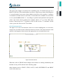
Figure 6.4 catalog in block diagram 6.2.2 ComConfig set Configure the baud rate, parity and stop bits settings of the RS-232 connection between
the host computer and the Scan controller. Changes will be reflected both the Scan
Controller and the host computer.
The figure 6.5 shows settings of baud rate, parity and stop bits. It can be found in
SubVIs from SC2000 driver.
Figure 6.5 Settings of baud rate, parity and stop bits
43
The default baud rate setting for RS-232 communication between the Scan Controller
and the Host computer is 2400. RS-232 supports baud rates up to 115200. If the
Command Line program is shut down, it will restart in its default setting of 2400 Baud.
Likewise, if the Scan Controller is power cycled, it will power up at its default baud rate
of 2400. If you choose to use a higher baud rate, you must reconfigure the system every
time when the program is restarted or the Scan Controller is power cycled. Failing to do
so will result in a communications error.
6.2.3 Correction of the Laser Position The command Position 0 0, which used to correct the Laser position can be written into
the G language. It works with the SubVIs. It takes the laser to (0, 0) position before we
start to scan.
6.3 Data process Click START button to scan the image-plate. When the scan is finished, we can save
the data or the intensity graph. Also we can scan more times just by click START
button. It makes automatically the position of laser to (0, 0) and start to scan. The
numbers in the array are not new value, but they are numbers which are added by old
and new value.
6.3.1 Mode and files options Figure 6.6 Front panel of mode and file options 44
The figure 6.6 shows front panel of mode and file options. We have two modes to scan
Image-Plate, NORMAL and FAST mode. For the running type we can choose
100mm*100mm or 10cm*10cm. The default measuring time is 50ms. It means the
laser is open for 50ms. We can change it according to need. Also we can save the data
into a file and load the data from a file after scanning. With the SHOW button we can
execute the data into the intensity graph. It is useable only in FAST mode.
There are three switches for laser, lamp and photomultiplier. When the laser switch is
on, the lamp switch is automatically off and unusable. Because when both switches
are open the photomultiplier will be broken immediately. Also when the lamp switch
is on, the laser switch is automatically off and unusable.
When the photomultiplier tube is on we can start to run this program, and stop at any
time. Also we can save the data when the program is finish and load old data to the
intensity graph to compare two graphs. We can also see the difference between two
selected graphs. It will be showed in the ALT graph and we can also save and print it.
The Difference button is useable after we load an old data. And Save Diff. button is
useable after we click Difference button.
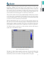
Figure 6.7 Intensity graph for current scan The figure 6.7 shows intensity graph for current scan. We can see the data on the
intensity graph and the sum of the whole data. The coordinate figure is changed
automatically, from the lowest number to the highest number in the graph.
45
Instead of text program writing as in the Command line Interface, Labview can also
write these graphically with the SubVIs (deltapositionxy.vi, wait.vi……).
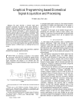
6.3.2 2D­array into intensity graph The data of each point from the memory should be read out and displayed into a graph.
We will get a 1D-array data, divided into a 2D-array for analysis.
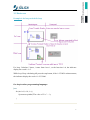
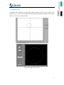
The figure 6.8 shows example how the 2D-Array is shown in an intensity graph. If
connect the array directly into the Intensity Graph, it just display the overturned graph
(left diagram). Then we should dispose this array with the Functions to be shown
correctly..
Figure 6.8 example of 2D-array into intensity graph
46
The figure 6.9 shows rotation of an array.
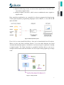
Figure 6.9 rotation of an array 6.3.3 Simulation Use stacked sequence structure to get the 2D array from the Voltmeter with DAQ
Assistant first, then analysis the array and display into an intensity graph.
Figure 6.10 The first structure 47
The figure 6.10 shows the first structure in which to get values from voltmeter. The
figure 6.11 shows the second structure in which to analyse the array and show in an
intensity graph.
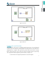
Figure 6.11 The second structure 6.3.4 Queue structure Figure 6.12 Block diagram of queue structure 48
The figure 6.12 shows block diagram of queue structure which is called
producer/consumer design pattern. It has one produce loop and one consumer loop. In
produce loop we can get measured values and put them into Enqueue function (Figure
6.13). In consumer loop we can get these values one by one through Dequeue
function and put them into an array and intensity graph (Figure 6.14).
Figure 6.13 Measured values go into Enqueue function For measuring pulse number in limited time (50ms), we use counter pinout of terminal
block (CB-68LP). Then put the data into the Enqueue function.
Figure 6.14 Consumer loop The elements will be dequeued into an array and an intensity graph.
49
6.3.5 Array The upper part of figure 6.14 shows how to build an array. To build an array we use a
Build vi (100*100). The initial numbers are all zero. When we get values from Dequeue
vi, we need replace zero to new values which we need. So we use a replace vi, and give
it coordinate (column and row) and value. To determine the coordinate for each value
we use Quotient&Remainder vi. According to quotient and remainder the dequeued
value is put in the correct position. For example, when i is 77, it is the 78th value,
because i starts from zero. 77 divided by 100 is 0 and we have 77 remainder. So this
value is put to the first row the 77th column. 6.3.6 Event structure The figure 6.15 is an event structure. It has one or more subdiagrams, or event cases,
exactly one of which executes when the structure executes. The Event structure waits
until an event happens, then executes the appropriate case to handle that event.
Figure 6.15 Event structure When the value of SHOW button changed, this structure is running immediately and
the data of array will be shown in the intensity graph.
Other buttons such as START, STOP, SAVE, LOAD, DIFFERENCE and PRINT
work in the same way.
50
Conclusions After several months’ experiments, I finished this design of the program for the Laser
scanner. It can be used to scan 100mm × 100mm large area or 10cm × 10cm and
basically achieved the expectant request.
Although the system never used to scan any Image Plate reality, and still need to
improve lots of things, but I really enjoyed the procedure and really learned a lot.
Thanks all the people that helped me during these months, especially Mr. Klaus
Bussmann, Mr. Peter Hiller, Prof. Dr. -Ing Christoph Helsper, Prof. Dr. Ulrich Rücker
and Mr. Schmitz Bethold.
Thanks for everything!
51
Appendix A. Mini SAX Command Input Characteristics
• Differential Voltage Range: ±3 volts differential for full scale
• Input Impedance: 5 KΩ differential
Position Output: ±3 volts differential for full scale
Power Input
• Voltage: ±15 to ±24 volts DC
• Quiescent Current: +170mA, -150mA
Motor Drive Power
• Dynamic Current max.: 2.5 Amps RMS
• Peak Current: 10.0 Amps
Note: U20/U21 mounting screws should be tightened to a torque of 16 in-lb (1.8
N-M).
Control I/O Characteristics
• Servo Ready: Open Drain, Active Low (50 mA max.)
• Servo Enable: TTL/CMOS Compatible, Active Low
• Temp OK*: Open Drain, Active Low (50 mA max.)
* Part of optional Temperature Controller Module
Protection
• Fully Fused: Motor Output, Automatic Gain Control, and Thermal Controller
• Automatic Shutoff: Over-position, Supply Undervoltage, Position Detector
Inactive
Temperature Range: 0°C to 50°C Operating
1
3
1
Size W x L x H (without mounting bracket): 2 ⁄ ” x 3 ⁄ ” x1 ⁄ ”
8
8
4
(54.5mm x 86.5mm x 31.35mm)
Weight: 66 grams (Includes all optional modules, without mounting bracket)
52
B. DAQ­Card 6024E General Product Name PCI-6024E
Product Family Multifunction Data Acquisition
Form Factor PCI
Part Number 777743-01
Operating System/Target Real-Time , Linux , Mac OS , Windows
LabVIEW RT Support Yes
DAQ Product Family E Series
RoHS Compliant No
Analog Input Channels 16 , 8
Single-Ended Channels 16
Differential Channels 8
Resolution 12 bits
Sample Rate 200 kS/s
Max Voltage 10 V
Maximum Voltage Range -10 V , 10 V
Maximum Voltage Range Accuracy 16.504 mV
Minimum Voltage Range -50 mV , 50 mV
Minimum Voltage Range Accuracy 0.106 mV
Number of Ranges 4
Simultaneous Sampling No
On-Board Memory 512 samples
Analog Output Channels 2
Resolution 12 bits
Max Voltage 10 V
Maximum Voltage Range -10 V , 10 V
Maximum Voltage Range Accuracy 8.127 mV
Minimum Voltage Range -10 V , 10 V
Minimum Voltage Range Accuracy 8.127 mV
Update Rate 10 kS/s
Current Drive Single 5 mA
Digital I/O Bidirectional Channels 8
Input-Only Channels 0
Output-Only Channels 0
Number of Channels 8
53
Timing Software
Logic Levels TTL
Input Current Flow Sinking , Sourcing
Output Current Flow Sinking , Sourcing
Programmable Input Filters No
Supports Programmable Power-Up States? No
Current Drive Single 24 mA
Current Drive All 192 mA
Watchdog Timer No
Supports Handshaking I/O? No
Supports Pattern I/O? No
Maximum Input Range 5 V
Maximum Output Range 5 V
Counter/Timers Counters 2
Number of DMA Channels 1
Buffered Operations Yes
Debouncing/Glitch Removal No
GPS Synchronization No
Maximum Range 0 V , 5 V
Max Source Frequency 20 MHz
Minimum Input Pulse Width 10 ns
Pulse Generation Yes
Resolution 24 bits
Timebase Stability 100 ppm
Logic Levels TTL
Physical Specifications Length 17.5 cm
Width 10.7 cm
I/O Connector 68-pin male SCSI-II type
Timing/Triggering/Synchronization Triggering Digital
Synchronization Bus (RTSI) Yes
54
C. Relays 1. ABB Relay General Information Extended Product Type: R600 RB121 5vdc
Product ID: 1SNA645034R2300
EAN: 3472596450342
Catalog Description: RB121 5vdc
Long Description: Screw relay RB121 5vdc : 5vdc input / 1SPDT 10 mA up to 6A with
led
Dimensions Product Net Width: 6 mm
Product Net Height: 70 mm
Product Net Depth: 67.5 mm
Product Net Weight: 0.02 kg
Environmental Ambient Air Temperature:
Operation -20 ... 70 °C
Storage -40 ... 80 °C
Certificates and Declarations (Document Number) Declaration of Conformity - CE: 1SND225042C1000
LR Certificate: LRS_0620042
Additional Information IIT Publishing Status: Level 0 - Information enabled
Invoice Description: RB121 5vdc
Minimum switching capacity [V/mA]: 12 / 10 volt per milliamp
Number of Auxiliary Contacts CO (SPDT): 1
Output Current Maximum (Iout): 6 A
Output Voltage (Uout): 250 V AC
Product Main Type: R600
Product Name: Relay module
Rated Control Supply Voltage (Us): 5 V DC
Recommended Screw Driver: 3.5 mm
Standards: CEI 947-7-1 / CEI 947-1 / CEI 1131-2 (in relevant parts) / CEI 60664-1 /
CEM : IRC 1000-4-2. 3. 4. 5. 6.
Wire Stripping Length: 9 mm
55
2. PhoenixContact Relay Input data Nominal input voltage UN
5 V DC
Input voltage range in reference to UN
0.8 ... 1.2
Switching threshold "0" signal in reference to UN ≤ 0.4
Switching threshold "1" signal in reference to UN ≥ 0.8
Typical input current at UN
5 mA
Typical response time
0.8 ms
Typical turn-off time
1.5 ms
Operating voltage display
Yellow LED
Type of protection
Protection against polarity reversal
Surge protection
Protective circuit/component
Polarity protection diode
Varistor
Transmission frequency
50 Hz
Output data Output nominal voltage range
12 V DC ... 300 V DC (Partition plate
PLC-ATP must be installed for
voltages larger than 250 V (L1, L2,
L3) between identical terminal points
in adjacent modules. Potential
bridging is then carried out with
FBST 8-PLC... or ...FBST 500...)
Limiting continuous current
1 A (see derating curve)
Voltage drop at max. limiting continuous current < 500 mV
Type of protection
Protection against polarity reversal
Surge protection
Protective circuit/component
Polarity protection diode
Varistor
Connection data Connection method
Screw connection
Stripping length
8 mm
Screw thread
M3
Conductor cross section solid min.
0.14 mm²
Conductor cross section solid max.
2.5 mm²
Conductor cross section stranded min.
0.14 mm²
56
Conductor cross section stranded max.
2.5 mm²
Conductor cross section AWG/kcmil min.
26
Conductor cross section AWG/kcmil max.
14
General data Width
6.2 mm
Height
80 mm
Depth
86 mm
Ambient temperature (operation)
-25 °C ... 60 °C
Ambient temperature (storage/transport)
-40 °C ... 85 °C
Mounting position
Any
Assembly instructions
In rows with zero spacing
Operating mode
100% operating factor
Inflammability class acc. to UL 94
V0
Name
Standards/regulations
Standards/regulations
IEC 60664
EN 50178
IEC 62103
Rated surge voltage / insulation
4 kV / basic insulation
Rated insulation voltage
300 V
Pollution degree
2
Surge voltage category
III
57
D. Command Reference ?FreeFlashSpace: Returns byte count of available flash memory.
?FreeRAMSpace: Returns byte count of available SRAM.
?ID: Return system revision information.
?OpticalCal
?Position: Return the current position on the given axis.
?Status: Returns error information and clears error state.
?Sync
?Temp
?TempOK
AbortPgm: Halts the currently running program and disables servos.
ComConfig: Configure RS-232 serial port parameters for communication.
CreateFlashPgm: The action of Create Flash Program is to initiate the storage
mechanism in the Scan Controller so that a program may be saved to non-volatile
memory on-board the Scan Controller.
CreatePgm: Store a Scan Controller program in volatile memory on-board the Scan
Controller.
DelayedLaserGate
DelayedSetFPS
DelayedSetOutputSignal
DelayedSetSync
DelayedUnSetSync
DeltaPosition: Set the position of the current axis relative to the currentposition.
DeltaPositionXY: Set the vector position relative to the current position.
DeltaSlew: Move smoothly on the current axis relative to the currentposition.
DeltaSlewXY: Move smoothly relative to the current vectorposition.
DeltaTweakAxis: Apply gain and offset deltas to subsequent raster operations.
DeltaTweakAxisXY: Apply gain and offset deltas to subsequent vector operations.
End: Marks the end of a Scan Controller program.
ExecutePgm: Commence the execution of the named program.
ExecuteRasterPgm
ExecBinPgm
ExecSerialNumber
ExitPgm: Use ExitPgm to terminate programs by having them fall through repeat and
waitsync [1-4] statements.
FlipExchangeAxis: Use FlipExchangeAxis to reverse the sense of one or both axis and
to interchange the command stream between X and Y.
Ifexecutepgm
Ifexecuterasterpgm
Iftempokexecutepgm
Iftempokexecuterasterpgm
LaserModeSetup
Nrepeat
58
PackMemory
Position: Set the absolute position of the current axis.
PositionXY: Set the absolute vector position.
Raster: Declare the target axis for subsequent single axis (raster) commands and place
the Scan Controller in raster mode.
ReleasePgm
Repeat: The Repeat command will cause the Scan Controller program flow to return to
the first instruction in the program where execution is repeated.
SaveConfigInFlash
SerialNumberSetup
SetAnalogOutput
SetConfigVar
SetFPS
SetGSS
SetLaserPower
SetMOFGains
SetMOFMode
SetMOFShift
SetOutputSignal
SetPWM
SetSetSyncDelay
SetSync
SetTicklePulses
SetUnsetSyncDelay
SetXPRGain
SetXPROffset
SetYPRGain
SetYPROffset
Slew: Move smoothly to the given absolute position on the current axis in the specified
number of tick counts.
SlewXY: Move smoothly to the given absolute vector position in the specified number
of tick counts.
TransformAxis: Apply rotation or skew transformation to vector motion commands.
TweakAxis: Apply gain and offset to subsequent axis operations.
TweakAxisXY: Apply gain and offset to subsequent vector operations.
UnSetSync
Vector: Place the Scan Controller in vector mode.
Wait: Pause execution for the given number of tick counts.
WaitPosition: Pause Scan Controller program execution until the commanded position
for the current axis is reached.
WaitPositionXY: Pause Scan Controller program execution until the commanded
position is reached.
WaitSync
59
References GSI LUMONICS SC2000 COMMAND REFERENCE
GSI LUMONICS SC2000 SUPPORT PROGRAMS MANUAL
GSI LUMONICS SC2000 USER MANUAL
GSI LUMONICS SC2000 QUICK START GUIDE
VM500 VM1000 & VM1500 USER’S MANUAL
MINI SAX USER MANUAL
DAQ 6023E/6024E/6025E USER MANUAL
HTTP://WWW. NI.COM /
HTTP://WWW. WIKIPEDIA.ORG/
HTTP://WWW.GSIG.COM/
HTTP://WWW. IOP. ORG/
HTTP://WWW. LABVIEW.COM/
HTTP://WWW.PRENHALL. COM/BISHOP/
HTTP://SEMIA. COM/ INNOVATE/DEVE_15.HTM/
HTTP://LABVIEW. BRIANRENKEN. COM/
HTTP://WWW. NOVASCIENTIFIC . COM/
HTTP://WWW.PHOENIXCONTACT.COM/
HTTP://WWW. ABB. COM/
60