Download SAPT2002 User Guide - University of Delaware Dept. of Physics

SAPT2002: An Ab Initio Program for Many-Body
Symmetry-Adapted Perturbation Theory Calculations
of Intermolecular Interaction Energies. Sequential and
parallel versions.
User’s Guide
Last updated: May 25, 2004
Robert Bukowski, Wojciech Cencek, Piotr Jankowski,
Bogumil Jeziorski, Malgorzata Jeziorska, Stanislaw A. Kucharski,
Alston J. Misquitta, Robert Moszynski, Konrad Patkowski,
Stanislaw Rybak, Krzysztof Szalewicz, Hayes L. Williams, and Paul E.S. Wormer
Department of Physics and Astronomy,
University of Delaware, Newark, Delaware 19716
Department of Chemistry, University of Warsaw,
ul. Pasteura 1, 02-093 Warsaw, Poland
May 26, 2004
1
Contents
1 Introduction
4
2 Short overview of theory
5
3 Downloading SAPT2002
8
4 Packages included in the distribution
8
5 Structure of ./SAPT2002 directory
9
6 SAPT installations at a glance
10
7 Installing SAPT2002
10
7.1
Compall installation script . . . . . . . . . . . . . . . . . . . . . . . . . . . . . . . .
11
7.2
Compall asymp installation script . . . . . . . . . . . . . . . . . . . . . . . . . . . .
14
7.3
Testing SAPT2002 installation . . . . . . . . . . . . . . . . . . . . . . . . . . . . .
14
8 Using SAPT2002 with different front-end packages
14
8.1
ATMOL1024 . . . . . . . . . . . . . . . . . . . . . . . . . . . . . . . . . . . . . .
14
8.2
CADPAC . . . . . . . . . . . . . . . . . . . . . . . . . . . . . . . . . . . . . . . .
15
8.3
GAUSSIAN . . . . . . . . . . . . . . . . . . . . . . . . . . . . . . . . . . . . . . .
15
8.4
GAMESS . . . . . . . . . . . . . . . . . . . . . . . . . . . . . . . . . . . . . . . .
16
8.4.1
Optional modification of GAMESS source . . . . . . . . . . . . . . . . . .
16
8.4.2
Required and recommended input options . . . . . . . . . . . . . . . . . . .
17
8.4.3
runGAMESS script . . . . . . . . . . . . . . . . . . . . . . . . . . . . . . . . .
18
8.4.4
Interface . . . . . . . . . . . . . . . . . . . . . . . . . . . . . . . . . . . . . .
19
Hondo-8 . . . . . . . . . . . . . . . . . . . . . . . . . . . . . . . . . . . . . . . . .
19
8.5
9 How to run SAPT2002
9.1
20
Calculations of integrals and SCF energies . . . . . . . . . . . . . . . . . . . . . . .
+
22
9.1.1
DCBS and DC BS approaches . . . . . . . . . . . . . . . . . . . . . . . . .
22
9.1.2
MCBS and MC+ BS approaches . . . . . . . . . . . . . . . . . . . . . . . . .
23
Input for post-Hartree-Fock part . . . . . . . . . . . . . . . . . . . . . . . . . . . .
28
9.2.1
Namelist TRN . . . . . . . . . . . . . . . . . . . . . . . . . . . . . . . . . . .
28
9.2.2
Namelist CCINP . . . . . . . . . . . . . . . . . . . . . . . . . . . . . . . . . .
30
9.2.3
Namelist INPUTCOR . . . . . . . . . . . . . . . . . . . . . . . . . . . . . . . .
30
9.3
How to read the output . . . . . . . . . . . . . . . . . . . . . . . . . . . . . . . . .
33
9.4
Submitting a sequence of SAPT2002 jobs . . . . . . . . . . . . . . . . . . . . . . .
34
9.2
2
9.5
Memory and disk requirements . . . . . . . . . . . . . . . . . . . . . . . . . . . . .
36
10 Description of some internal data sets
39
11 Performance of SAPT2002
41
12 Tests and example input and output files
42
12.1 The examples directory . . . . . . . . . . . . . . . . . . . . . . . . . . . . . . . . .
42
12.2 Running tests jobs . . . . . . . . . . . . . . . . . . . . . . . . . . . . . . . . . . . .
44
13 Parallel SAPT: psapt2K2
46
13.1 Structure of ./psapt2K2 directory . . . . . . . . . . . . . . . . . . . . . . . . . . .
47
13.2 Installing psapt2K2 . . . . . . . . . . . . . . . . . . . . . . . . . . . . . . . . . . . .
48
13.2.1 compall installation script
. . . . . . . . . . . . . . . . . . . . . . . . . . .
48
13.2.2 Testing psapt2K2 installation . . . . . . . . . . . . . . . . . . . . . . . . . .
49
13.3 Using psapt2K2 with GAMESS as a front-end . . . . . . . . . . . . . . . . . . . . .
49
13.4 How to run psapt2K2 . . . . . . . . . . . . . . . . . . . . . . . . . . . . . . . . . .
51
13.4.1 Running psapt2K2 on SGI . . . . . . . . . . . . . . . . . . . . . . . . . . . .
52
13.4.2 Running psapt2K2 on an SP3/SP4 . . . . . . . . . . . . . . . . . . . . . . .
54
13.4.3 Running psapt2K2 on a Beowulf cluster . . . . . . . . . . . . . . . . . . . .
54
13.5 Input files . . . . . . . . . . . . . . . . . . . . . . . . . . . . . . . . . . . . . . . . .
62
13.6 Memory and disk requirements . . . . . . . . . . . . . . . . . . . . . . . . . . . . .
63
13.7 Electrostatics, dispersion, and induction (EDI) from monomer properties . . . . . .
63
13.7.1 The pEDI scripts . . . . . . . . . . . . . . . . . . . . . . . . . . . . . . . . .
65
13.7.2 Calculating electrostatics, induction, and dispersion from fitted monomer
electron densities and susceptibility functions . . . . . . . . . . . . . . . . .
68
A Appendix: Integral/SCF interfacing
73
B Appendix: List of subroutines
73
C Appendix: Input/Output files for the example BER (Be2 )
83
D Appendix: Capabilities of pcksdisp program
88
E Appendix: Generation of auxiliary basis
91
3
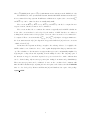
1
Introduction
SAPT2002 is a computer code implementing the many-body version of Symmetry-Adapted Perturbation Theory (SAPT). SAPT is designed to calculate the interaction energy of a dimer, i.e.,
a system consisting of two arbitrary closed-shell monomers. Each monomer can be an atom or
a molecule. The “many-body” phrase used in the title refers to electrons as “bodies”, like in
the name Many-Body Perturbation Theory (MBPT). In SAPT, the interaction energy is expressed as a sum of perturbative corrections, each correction resulting from a different physical effect. This decomposition of the interaction energy into distinct physical components is a
unique feature of SAPT which distinguishes this method from the popular supermolecular approach.
The SAPT methodology and its applications are discussed in several review papers
[1, 2, 3, 4] where complete references to the original developments can be found. The set of
formulas programmed in SAPT2002 is included in the paper published in the book accompanying the METECC collection of computer codes [5]. The METECC paper is available on the SAPT
web page http://www.physics.udel.edu/∼szalewic/SAPT/SAPT.html and can be also found in
the SAPT2002 distribution ( SAPT2002/doc/METTEC.ps).
The METECC project [5] was the first distribution of the SAPT codes. The next version of
SAPT, called SAPT96 [6], was available since 1996. Compared to SAPT96, the current version,
SAPT2002, is about a factor of two faster in medium size (about 200 functions) bases. It also
allows calculations with up to 1023 basis functions (SAPT96 was restricted to 255), is interfaced
with a larger number of front-end SCF packages, and runs on a larger number of platforms. A
parallel version of SAPT2002 has also been developed, which will be referred to as psapt2K2.
This version runs on SGI Origin, IBM SP, and on Linux clusters and scales well up to about 32
processors. See Sec. 13 for detailed description of this version.
A version of SAPT has also been developed [7, 8, 9] which allows calculations of the nonadditive portion of the interaction energy for an arbitrary trimer consisting of closed-shell monomers.
Thus, SAPT can now be used to calculate the two leading terms in the many-body expansion of the
interaction energy of a cluster, (where “bodies” here are monomers). The programs implementing
the three-body SAPT can be obtained by a special request.
The calculation of the interaction energy of a dimer using SAPT2002 involves four steps. In
the first step, one and two-electron integrals are computed in a chosen orbital basis set and then
SCF calculations are performed on both monomers. The SCF calculation for the dimer can be also
performed at this stage. Several integral/SCF packages are interfaced to SAPT and can be used,
including free packages such as GAMESS [10]
(see http://www.msg.ameslab.gov/GAMESS/GAMESS.html) and ATMOL [11] (a modified version
of the latter package, ATMOL1024, is included in SAPT2002 distribution and can be down-
4
loaded from SAPT web page). After the SCF calculations are completed, the “atomic” integrals
(i.e., integrals between functions of the basis set) are transformed into molecular integrals using
scalable the 4-index transformation program tran. In the third step, the Coupled-Cluster (CC)
program ccsdt is invoked to calculate the MBPT and/or CC amplitudes for monomers A and B.
Finally, the sapt program is run to compute the interaction energy components. Several short
interface programs are also invoked between calls to tran and ccsdt. The computational cost of
the SAPT corrections scales as a product of some powers of the number of occupied orbitals and
of the virtual orbitals. Therefore, with a given basis set size, calculations for larger systems will
take longer. At the present time (beginning of the year 2003), the largest runs performed included
about 500 (300) virtual orbitals for systems with monomers containing about 10 (20) occupied
orbitals. Routine runs typically use basis set of about 200 functions.
In the asymptotic region, (i.e., for large intermonomer separations), SAPT calculations may be
significantly simplified by means of the multipole expansion which allows to express the interaction
energy as a series of inverse powers of intermonomer separation. Coefficients of this series, the socalled van der Waals constants, depend only on monomer multipole moments and polarizabilities
(static and dynamic) and can be computed using the POLCOR suite of codes by Wormer and
Hettema [12]. The POLCOR suite, as well as a fitting program developed in our group and
utilizing the ab initio asymptotic information, comprise the independent package asymp SAPT,
distributed optionally with SAPT2002.
This document is intended to provide a basic introduction to the SAPT method and the
instructions on how to download, compile, and run the SAPT2002 and psapt2K2 codes. Also
included are some details on the types of computers, compilers, and integral plus Hartree-Fock selfconsistent field (SCF) packages that SAPT has been tested with. Whereas extensive tests of SAPT
have been performed, there may appear unforeseen difficulties with the installation and running
of the codes. As SAPT2002 and psapt2K are products of a research project, no resources are
available to provide support for users. The authors of the code will try to provide a limited help
within the restrictions of their schedules.
2
Short overview of theory
In SAPT, the total Hamiltonian for the dimer is partitioned as H = F +W +V where F = F A +FB is
the sum of the Fock operators for monomers A and B, V is the intermolecular interaction operator,
and W = WA +WB is the sum of the Møller-Plesset fluctuation operators. The latter operators are
defined as: WX = HX − FX , where HX is the total Hamiltonian of monomer X. The interaction
5
energy, Eint , is expanded as a perturbative series
Eint =
∞
∞ X
X
(nj)
(nj)
(Epol + Eexch )
(1)
n=1 j=0
with the indices n and j denoting the orders in the operators V and W , respectively. The polar(nj)
ization energies Epol are identical to the corrections obtained in a regular Rayleigh-Schrödinger
(nj)
perturbation theory. The exchange corrections Eexch arise from the use of a global antisymmetrizer
to force the correct permutational symmetry of the dimer wave function in each order, hence the
name “symmetry adaptation”.
(1j)
The polarization corrections of the first order in V , Epol , describe the classical electrostatic
(1j)
interaction and are denoted by Eelst . The second-order corrections can be decomposed into the
induction and dispersion parts:
(2j)
(2j)
(2j)
Epol = Eind + Edisp
(2j)
(2j)
(2j)
Eexch = Eexch−ind + Eexch−disp .
and
(2)
The induction component is the energy of interaction of the permanent multipole moments of one
monomer and the induced multipole moments on the other, whereas the dispersion part comes
from the correlations of electron motions on one monomer with those on the other monomer.
The SAPT interaction energy can be computed at different levels of intramonomer correlation
and an approximate correspondence can be made between these levels and the correlation levels of
the supermolecular methods. It can be shown [13], for example, that the sum of the polarization and
exchange corrections of the zeroth order in W provides a good approximation to the supermolecular
HF
Hartree-Fock interaction energy, Eint
:
(10)
(10)
(20)
(20)
HF
HF
Eint
= Eelst + Eexch + Eind,resp + Eexch−ind,resp + δEint,resp
,
(3)
HF
, defined by the equation above, collects all the third- and higher-order induction
where δEint
and exchange-induction terms. The subscript “resp” means that the coupled Hartree-Fock-type
response of a perturbed system is incorporated in the calculation of this correction. Including
the intramonomer correlation up to a level roughly equivalent to the supermolecular second-order
MBPT calculation, we obtain the interaction energy referred to as SAPT2:
(12)
(1)
(22)
(20)
(22)
(20)
SAPT2
HF
Eint
= Eint
+ Eelst,resp + exch (2) + tEind + tEexch−ind + Edisp + Eexch−disp
where the notation (n) (k) =
(20)
(22)
Pk
j=1
(22)
(4)
(22)
E (nj) has been used, tEind is the part of Eind not included in
(22)
Eind,resp , and tEexch−ind is the estimated exchange counterpart of tEind
t (22)
Eexch−ind
(20)
≈ Eexch−ind,resp
t (22)
Eind
.
(20)
Eind,resp
(5)
The highest routinely-used level of SAPT, approximately equivalent to the fourth-order of
supermolecular MBPT theory, is defined by:
(13)
(1)
(1)
(2)
SAPT
SAPT2
Eint
= Eint
+ Eelst,resp + [exch (CCSD) − exch (2)] + disp (2),
6
(6)
(1)
(1)
where exch (CCSD) is the part of exch (∞) with intramonomer excitations at the CCSD level only.
The SAPT2 level of theory takes much less time than the full SAPT calculations and therefore
(22)
it is recommended for large systems. If still faster calculations are required, the corrections tEind
(20)
and Eexch−disp can be omitted as these are usually fairly small.
(20)
(20)
(12)
(13)
The corrections Eind,resp , Eexch−ind,resp , Eelst,resp , and Eelst,resp can also be computed in nonresponse versions, but these forms are not recommended.
The corrections listed above constitute the current set typically used in SAPT calculations.
A few other corrections have been developed by the authors of SAPT but these are either not
working in the current version of the program or for some other reasons are not recommended to
(14)
(122)
be computed. These corrections include Eelst,resp [14], Eelst
[14], higher-order approximations to
the electrostatic interaction [15], the dispersion energy at the CCD level [16], and some corrections
of third-order in V [17].
At intermonomer separations R large enough for the exchange effects to be negligible, the
SAPT results become identical to those of the regular Rayleigh-Schrödinger perturbation theory. The calculation of the interaction energies in this region can be substantially simplified by
neglecting the overlap effects and expanding V in the multipole series. The long-range part of
the interaction energy becomes then expressed as a power series in R −1 , with coefficients that
can be obtained using only monomer properties (viz. multipole moments and polarizabilities).
These monomer properties can be calculated ab initio at the correlation level consistent with
finite-R SAPT calculations [18, 19] using the monomer parts of the basis set and the POLCOR
suite of codes developed by Wormer and Hettema [12] and distributed as a part of the package
asymp SAPT.
7
3
Downloading SAPT2002
The SAPT20020 distribution, the parallel version psapt2K2, the asymp SAPT asymptotic
package, and theATMOL1024 SCF code can be obtained from the web page
http://www.physics.udel.edu/∼szalewic/SAPT/SAPT.html.
All these codes are distributed free of charge but we require users to sign a license agreement
which can be downloaded from this web site and mailed or faxed to us as described there. We will
then email to the interested party the password needed to complete the download. The users who
download the asymp SAPT and ATMOL1024 modules will be also asked to notify the authors
of ATMOL and POLCOR suites of the intended use of their codes.
4
Packages included in the distribution
Currently there are five options for downloading SAPT2002 and the accompanying programs:
1. SAPT2002 (size of about 2.1 Mbyte). This file contains only the SAPT2002 codes. You
will have to obtain some integral/SCF package (like GAMESS, CADPAC, GAUSSIAN,
etc.) or download the ATMOL1024 code (see below) before running SAPT2002. On
decompression, this file expands into ./SAPT2002/.
2. ATMOL1024 (size of about 0.14 Mbyte). This file contains the ATMOL1024 package.
This package is a subset of the ATMOL code [11] modified by us to handle basis sets of up
to 1023 orbitals. On decompression, this file expands into ./SAPT2002/atmol1024, so please
decompress it in the root directory that SAPT2002 is in!
3. asymp SAPT (size of about 2.4 Mbyte). Contains the POLCOR suite [12] and the accompanying programs necessary for computation of asymptotic coefficients. Also included
is the potential energy fitting program genfit v1, developed in our group. On decompression this file expands into ./asymp SAPT/. Documentation for this package is located in
./asymp SAPT/doc.
4. COMPLETE SET OF SEQUENTIAL CODES (size of about 4.8 Mbyte)
This file contains all the above modules. On decompression it expands into ./SAPT2002/
and ./asymp SAPT/.
5. psapt2K2 (size of about 7 Mbyte)
Contains the parallel version of the SAPT codes, psapt2K2. To make the most of this
version, you will have to obtain and install GAMESS(US) as the integral/SCF package.
See Sec. 13 for detailed description of psapt2K2.
8
The instructions on unpacking these files can be found on the SAPT web page in the Download
Area.
5
Structure of ./SAPT2002 directory
After unpacking, the ./SAPT2002 main directory will contain the following files and subdirectories:
• Cleandirs: use this script to clean the entire SAPT2002 directory tree before recompiling
from scratch.
• Compall: script used to build the package (see Sec. 7).
• Makefile: a generic makefile used by Compall.
• UPDATES.log: log of the history of changes and updates.
• atmol1024/: present if ATMOL1024 file has been downloaded, this directory contains the
sources of the ATMOL1024 SCF code.
• tran/: program performing the one- and two-electron integral transformation.
• cc/: program performing the coupled cluster singles and doubles calculations for the monomers.
The first few iterations are performed perturbatively, in this way producing MBPT orderby-order amplitudes needed in SAPT. Both CCSD and MBPT amplitudes are later used
by sapt module to compute intramonomer correlation contributions to various interaction
energy components.
• sapt/: program computing the SAPT corrections.
• misc/: contains various interface and utility programs. Most integral/SCF packages need an
interface program to extract one-electron integrals and SCF orbital energies and coefficients
from files created by these packages and transform them into a standard form readable by
the transformation code (two-electron integrals are read by transformation directly without
such preprocessing). Other programs present in misc/ include int and sort, interfacing the
transformation to coupled cluster code, memory estimator memcalc, and a set of geometry
converters which can be used with the bin/Runlot* scripts for automatic generation of
potential energy surfaces (see Sec. 9 for details).
• bin: utility scripts for running SAPT. After compilation, this directory will also contain the
executables used in a SAPT run.
9
• doc: documentation for SAPT2002; contains this document and the METECC paper [5]
in the postscript form. Documentation for asymp SAPT can be found in that package in
the directory asymp SAPT/doc/.
• examples: input and output files for a set of systems and a variety of integral/SCF packages.
This is a good source of templates for your runs.
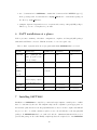
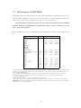
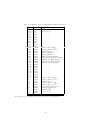
6
SAPT installations at a glance
Table 1 presents a summary of hardware configurations, compilers, and integral/SCF packages
with which SAPT has been tested. This list is meant to be used as a guide only.
Table 1: Grid of systems and front-end programs with which SAPT2002 has been tested
machine
ATMOL1024
GAMESS(US)
CADPAC
GAUSSIAN98
SGI OnK
Ok.
Ok.
Ok.
Ok.
(although AT-
MOL properties have
some problems)
Linux and
Ok.
Ok.
Ok.
Ok.
g77
Linux and
Ok.
GAMESS does
Ok.
Ok.
Ok.
Ok.
Not checked.
RS/6000
but works under g77.
Ok.
Ok.
Not checked.
Not checked.
SUN
Ok.
Ok.
Not checked.
Not checked.
PGF77
not work.
(3.3.2)
Alpha
Doesn’t
work
under Compaq compiler
7
Installing SAPT2002
Installation of SAPT2002 is controlled by a universal script Compall, a small portion of which
has to be customized by the user. The Compall script sets the compilation options appropriate for
the hardware platform and for the integral/SCF interfaces chosen. It then compiles and links all
the pieces of the code, which sometimes requires access to the I/O libraries of the integral/SCF
packages. If ATMOL1024 has been downloaded and the ./SAPT2002/atmol1024 directory is
present, this package is also built. Finally, Compall updates the scripts used to run SAPT2002
10
(SAPT, Runlot*) by inserting updated paths to executables. (The asymp SAPT package is
installed by a separate script).
7.1
Compall installation script
The following adjustments must be made by the user to the Compall script:
1. Execution shell: Change the first line of the script to one of the following:
• #!/bin/bash : The BASH shell on a LINUX box, or
• #!/bin/ksh : The Korn shell on all other platforms
2. Integral/SCF program: Declare the SCF packages you wish SAPT2002 to be interfaced with. In addition to the SCF front-ends listed in Compall, we know that other users
have interfaced SAPT with DALTON and MOLPRO, but these interfaces are not yet
available in SAPT2002. An integral/SCF package is activated by simply setting the corresponding variable in the script to the complete path to the directory where the libraries
(or executables, depending on the SCF package) of a given package are located (for example,
GAMESS=/home/local/gamess). Otherwise set the variable to ‘NO’ (note the capitals). In
addition, for GAMESS, the so-called “version number”, VERNO=XX, needs to be specified
(SAPT2002 assumes that the name of the GAMESS executable is gamess.$VERNO.x).
The list of SCF codes included in Compall does not include ATMOL1024. This latter
option is activated automatically if ATMOL1024 has been downloaded and is present in
the ./SAPT2002/atmol1024 directory. Thus, you may set all the integral/SCF variables
to ‘NO’, provided that ATMOL1024 has been downloaded. Otherwise at least one integral/SCF variable must be set by specifying the path. If ATMOL1024 is present and in
addition one or more integral/SCF packages are selected, both ATMOL1024 and the explicitly selected interfaces should work with the created SAPT2002 executables. In most
cases, the SAPT2002 codes use I/O libraries of the integral/SCF packages in order to read
the data created by these packages. Therefore, a given SCF package has to be installed
before SAPT2002 and its libraries must be accessible. Two exceptions are CADPAC and
GAMESS, both of which generate data read by SAPT2002 using its own subroutines. The
possible SCF programs that can be used to generate atomic integrals and SCF vectors for
SAPT2002 are
• ATMOL1024: This is the current and maintained version of ATMOL [11], extended
to handle up to 1023 basis functions. ATMOL1024 is the default integral/SCF package. The Compall script checks if ATMOL1024 source is present in ./SAPT2002/atmol1024
subdirectory and compiles it automatically. (If for some reasons ATMOL1024 has to
11
be kept in another location, and compiled separately, it can still be used by SAPT2002
if the line ATMOL1024=NO in Compall is changed to reflect the current location of the
ATMOL1024 main directory.) ATMOL1024 code has been tested with SAPT2002
more extensively than any other package and is the recommended choice. Another
package with which SAPT has been extensively tested is GAMESS(US), which also is
currently the only parallel front-end for parallel version of SAPT.
• GAUSSIAN: GAUSSIAN94 (G94) and GAUSSIAN98 (iG98). Set at least one of
these variables to NO as these packages are mutually exclusive. The path specified here
should contain the GAUSSIAN’s library util.a (usually it is main directory of the
GAUSSIAN distribution).
• GAMESS: If used, set the path to wherever the GAMESS executable is located. Also
set the variable VERNO which is the middle part of the name ofthis executable (e.g., for
gamess.01.x, VERNO=01). The sole purpose of the variable GAMESS in Compall is to pass
the path and name of GAMESS executable to the SAPT execution script. No access is
needed to any GAMESS files at the compilation time. Thus, compilation will proceed
even if GAMESS is not installed on your system beforehand.
• CADPAC: This package does not need any interface programs since the files created
by it can be read directly by SAPT2002 codes. Also, SAPT2002 does not need acess
to any CADPAC libraries, so that the compilation will proceed even if CADPAC is
not installed on your system.
• ACES: This interface has not been tested recently but should work.
• ALCHEMY, HONDO, MICROMOL: These packages have not been in use for a
long, long time and the interfaces to them may be not working. Should you choose one
of these, we would be interested in knowing if it works.
It is also possible to build the SAPT2002 package for use with the older version of ATMOL
(such a version, limited to 255 basis functions, is included in the asymp SAPT distribution).
This can be accomplished by setting the variable ATMOL in Compall equal to the path of the
main ATMOL directory (change the line ATMOL=NO) and removing or renaming the directory
./SAPT2002/atmol1024 (if present). The ATMOL package has to be compiled prior to the
compilation of SAPT2002. SAPT2002 cannot be interfaced with ATMOL1024 and
ATMOL simultaneously.
3. PLATFORM: Two variables need to be set:
• TARGET is the system on which SAPT2002 will be compiled. This can be one of
(all lower case): sgi, ibm32, ibm64, alpha, g77, pgf77, or sunf90. sgi stands
12
for the Silicon Graphics ORIGIN or POWER CHALLENGE series computers with the
MIPSPRO 7.3 or higher compiler; ibm32 – for the IBM RS6000 or SP machines (on
64-bit IBM platforms ibm64 can be also tried, but sometimes it causes problems with
dynamic memory allocation); alpha – for the (formerly DEC) ALPHA platform; g77
and pgf77 – for a LINUX box with the G77 or PGF77 compilers, respectively; sunf90
– for the Sun SPARC machine equipped with the FORTRAN90 compiler.
• BLAS points to the Basic Linear Algebra Subroutine library that is to be used. The
BLAS library is installed on most Unix computers. On SGI, IBM RS6000, and LINUX
machines set BLAS=’ -lblas ’. On an ALPHA, set BLAS=’ -ldxml ’; on IBM SP –
BLAS=’ -lessl ’; and on SPARC – BLAS=’ -xlic lib=sunperf ’. If you have compiled yourself a self-optimizing BLAS library like ATLAS, set BLAS=’ -L<Full Path
to Library> -latlas ’.
4. 64-bit GAMESS: if you intend to use GAMESS compiled with a 64-bit integer (this
happens by default on the ALPHA platform, but may also happen on SGI when “sgi64” is
specified during compilation of GAMESS), replace the line GAMSI8=NO with GAMSI8=YES.
SAPT2002 compiled in this way may not work correctly with other SCF front-ends, in
particular with GAUSSIAN).
Once all the variable mentioned above are set, simply type:
• C-Shell users: ./Compall >& compall.log &
• K-Shell users: ./Compall > compall.log 2>&1 &
and compilation should begin. Check compall.log to see if all is well. The Compall script will
create a file ‘./SAPT2002/stamp.intf’ containing a summary of the settings you have used in the
compilation. A subsequent invocation of Compall will detect any changes made to these settings
since stamp.intf was last created and only those parts of the code will be rebuilt which were
affected by these changes. Running the script ./SAPT2002/Cleandirs will restore the ./SAPT2002
directory to its “distribution” state, i.e., all object files and executables (except shell scripts) will
be deleted and invocation of Compall will start the compilation from scratch.
One more customization step may be required before SAPT2002 is run with GAMESS as
the SCF fron-end: the ./SAPT2002/bin/runGAMESS script must be modified by setting the TARGET
variable, which depends on the platform and on the way GAMESS has been compiled. In most
cases, the default TARGET=sockets will be appropriate, although on SGI machines TARGET=sgi-mpi
is also popular. Consult your local GAMESS installation. Further customization of runGAMESS
will be needed for other targets (if you need to do such a customization – see examples given in
both runGAMESS and the standard rungms for the GAMESS distribution).
13
7.2
Compall asymp installation script
If you have downloaded the asymp SAPT package, it will expand into ./asymp SAPT directory.
Change to this directory and use Compall asymp script to build all programs in this package. The
subdirectory doc contains the user’s manual for these programs. The asymptotics calculations are
presently limited to 255 orbitals and the relevant codes are interfaced only with the older version
of ATMOL (included in asymp SAPT package).
7.3
Testing SAPT2002 installation
Once the compilation has been completed successfully (if unsure, just grep the compall.log file
for the word error), we strongly recommend that you perform as many tests as is possible before
starting to use SAPT2002 for production runs. A suite of test jobs of varying size and for various
SCF front-ends has been provided for this purpose in sub-directory examples/. Sample outputs
from different platforms can be also found there. For more information on running the test jobs –
see Sec. 12.
8
8.1
Using SAPT2002 with different front-end packages
ATMOL1024
A good place to look for the description of input to ATMOL1024 is Paul Wormer’s web page,
http://www.theochem.kun.nl/∼pwormer (strictly speaking, this is a description of the older version of ATMOL, but the input options are the same as for ATMOL1024). Below we discuss
several options relevant for a SAPT2002 run.
It is convenient to reduce outprints from the integral (integw) module of ATMOL1024
by adding the directive NOPRINT GROU GTOS to the “intinp” files. This will suppress printing
of the groups or ordered GTOs. Adding the word BASI to the list will also suppress the basis set outprint. To avoid calculation of the multipole integrals, not needed in a SAPT calculation, include the directive BYPASS PROPERTY (this may be important especially on SGI machines, where the absence of such directive may cause a run-time error). Inclusion of a line
FPRINT NVCT NEIG NFTE NITE NPOP in the *.scfinp input files will ask the scf program to
skip the outprint of the vectors, eigenvalues, Fock trial matrix, iterations, and populations for that
run.
When the supermolecular SCF interaction energy is calculated during a SAPT run, i.e., when
the scfcp option is in effect (most runs are like this), the files nameA.intinp and nameB.intinp
shouldcontain the directive BYPASS TWO to avoid recalculation of two-electron integrals. This directive should not be present in the file name.intinp or, in the case of a MC + BS calculation – in
14
nameMA.intinp and nameMB.intinp (name denotes here the name of the job). If the supermolecular SCF calculations are not performed, i.e., if the scfcp option is not in effect, then the directive
BYPASS TWO must be also removed from the file nameA.intinp. See Sec.1 9 for further explanation.
On Linux platforms with g77 compiler (except possibly for its latest verisons) there is a
restriction on the size of the file which cannot exceed 2 Gbytes. In such a case, if the two-electron
integral file generated by ATMOL1024 exceeds this size, it has to be split into several pieces each
2 Gbytes or less. For example, if the integrals are anticipated to take 5 Gbytes of disk space, one
should have them distributed over at least three files. This can be done by specifying
MAINFILE MT3 MT4 MT5
MAXBLOCK 499999
in the *.intinp files, somewhere below the basis set specification but before the ENTER directive.
The first of the lines above means that the files called MT3, MT4, MT5 will be used to store the
integrals, and that the size of each will not exceed MAXBLOCK*511*8 bytes, which in this case
amounts to somewhat less than 2 Gbytes (the number 511 comes from some internal data structures
of ATMOL1024). Now we have to tell the transformation module of SAPT2002 how many files
ATMOL1024 produced by including NMFILES=3 in the TRN namelist in the *P.data input file (see
Secs. 9 and 9.2 for description of this file). Of course, the number “3” would have to by changed if
some other number of MT* files were used. ATMOL1024 and SAPT2002 support up to 18 such
files, MT3 through MT20.
8.2
CADPAC
First notice that CADPAC can use only Cartesian basis functions. Also, currently, only angular
functions up to f are allowed. The input file used for CADPAC runs must include the SAPT
keyword. This keyword makes CADPAC write out to a file the SCF vectors and other information
in the format required by the SAPT2002 transformation code tran. Thus, there is no interface
program required for CADPAC.
Due to the large number of density-functional theory (DFT) eXchange Correlation (XC)
functionals implemented in CADPAC, this is a good program to use if the SAPT method based
on Kohn-Sham orbitals and orbital energies [SAPT(KS)] [20, 21] is to be applied.
To run SAPT2002 with CADPAC as a front-end, a special script /SAPT2002/bin/SAPT CADPAC
should be used instead of SAPT used for all other SCF programs.
8.3
GAUSSIAN
When using GAUSSIAN with SAPT2002, a symbolic link in the compilation script Compall
is made to point to the util.a file in the GAUSSIAN directory structure. The transformation
15
module tran of SAPT2002 links to this library to be able to read the rwf and two electron
integral files.
If for some reason GAUSSIAN92 were to be used, the GAUSSIAN94 interface can be
easily modified for this purpose. The only parameter that has to be changed is the number of
words read from disk in the program misc/g94intf.f. Specifically, line 243 which currently looks
like
CALL FILEIO(2, 501, 1000, T, 0)
has to be changed to
CALL FILEIO(2, 501, 32, T, 0)
so that the read does not go past the end of the file.
In GAUSSIAN94 and in higher versions of this code, the default method of SCF calculation
was changed to direct (two-electron integrals calculated in-core and not stored to disk). Since
SAPT2002 always needs the two-electron integrals, the command SCF=(CONV), which stands for
“do conventional SCF”, must be used to force the two-electron integrals to be written to disk. We
recommend SCF=(TIGHT,CONV) command to be used to tighten the SCF iterations convergence
criteria.
On IBM RS/6000 and SP type computers under various versions of the operating system,
GAUSSIAN is apparently using two different strategies to equivalence integer and real numbers
for the purpose of packing the integrals. These two possibilities can be accounted for by setting
the intpwp variable in the file tran/intpwp.f to 1 or 2. This variable stands for the number of
integers per “working precision word”. On older systems the “working precision word” was 4-byte
long (32-bit architecture) and for newer ones it is 8-byte long (64-bit architecture). GAUSSIAN
choices for what constitutes a working precision word on IBM computers seem to be sometimes
not related to hardware architecture.
Note that for unknown reasons, when using the GAUSSIAN series of codes, at least MBPT2
(MP2) level of theory must be requested to correctly close the files.
Also, we remind the user that the MASSAGE keyword should be used in GAUSSIAN when
setting the charges to zero (e.g., to perform an SCF run for a monomer in a dimer-centered basis
set).
8.4
8.4.1
GAMESS
Optional modification of GAMESS source
In order to ensure that the SCF energies from GAMESS are printed with a sufficient number of
decimals, we recommend one FORMAT change in the rhfuhf.src module, prior to compilation of
16
GAMESS. In the subroutine RHFCL, the statement
8000 FORMAT(’--- CLOSED SHELL ORBITALS --- GENERATED AT ’,3A8/10A8/
*
’E(’,A,’)=’,F20.10,’, E(NUC)=’,F16.10,’,’,I5,’ ITERS’)
should be replaced by:
8000 FORMAT(’--- CLOSED SHELL ORBITALS --- GENERATED AT ’,3A8/10A8/
*
8.4.2
’E(’,A,’)=’,F24.16,’, E(NUC)=’,F16.10,’,’,I5,’ ITERS’)
Required and recommended input options
Please note that standard (non-direct) SCF calculations must be performed and some options in
the GAMESS input must have specific values:
• In the $CONTRL input group, NOSYM=1 option must be present (i.e., no symmetry must be
requested).
• In the $INTGRL input group, NOPK=1 (integrals must not be in supermatrix form) and NINTMX=2048
options must be present. Maximum number of integrals in a record block NINTMX must
be the same as linrec variable in the SAPT2002 module trans.f which is set in the
IF(isitgams) THEN block. The linrec is currently set to 2048 (but can be changed to a
different value).
• We recommend that the following thresholds for the two-electron integrals, linear dependence,
and SCF convergence are set instead of the GAMESS default values:
– in the $CONTRL input group, ICUT=24, ITOL=26
– in the $CONTRL input group, QMTTOL=1.0E-30; this will prevent GAMESS from unexpectedly removing quasi-linearly dependent combinations of basis functions from the
variational space (at this point SAPT2002 does not work well if such a removal occurs)
– in the $SCF input group, NCONV=9.
• We recommend using the option ISPHER=1 in the $CONTRL input group, which forces GAMESS
to do SCF calculations in the basis set of spherical Gaussians instead of the default Cartesian
ones and thus reduces the risk of linear dependencies. Unfortunately, although using this
option reduces the dimension of the variational space available to the system, the atomic
integral file produced by GAMESS remains “Cartesian” and thus its size is not reduced.
• In the MC+ BS-type run (see Sec. 9 for explanation), the variable SPHG in the namelist TRN
in the *P.data file (see Secs. 9 and 9.2for detailed description of this file) must be set to F
17
or .FALSE., even if GAMESS was run with ISPHER=1. This is because of the “Cartesian”
character of the integrals file, as mentioned above. The variable SPHG, which defaults to
.TRUE. (i.e., spherical basis is assumed), is only important for MC + BS and MCBS runs and
has no effect in the DCBS case.
8.4.3
runGAMESS script
Whereas most other integral/SCF packages are invoked in the SAPT script by just executing a
given program, GAMESS needs its own script, ./SAPT2002/bin/runGAMESS, called from the
SAPT script. runGAMESS is a slightly modified version of the standard script rungms distributed
with GAMESS. As already pointed out in Sec. 7, the user must edit this script and supply the
appropriate value of the TARGET variable. The targets sockets and sgi-mpi have been extensively
tested, while other targets may require some additional customization to make GAMESS run.
These additional changes are independent of SAPT2002-related portions of runGAMESS and, if
needed, can be introduced with the help of the standard GAMESS documentation.
If you rather prefer your own GAMESS script instead of runGAMESS, you can easily adapt
it for use with SAPT2002 by following these steps:
• Copy your script into the ./SAPT2002/bin directory. In the SAPT script, change the name
of runGAMESS to that of your own script.
• The SAPT script communicates with runGAMESS (or your custom-made script) through the
syntax of the type
runGAMESS $JOB $VERNO $NNODES $SCR $PUNCHDIR $GMSPATH
where
– JOB is the name of the input file, like xxx.inp, give only the xxx part
– VERNO is the “version number” of the executable (usually the name of the executable is
something like gamess.$VERNO.x)
– NNODES is the number of compute processes to be run (only 1 can be used with sequential
SAPT2002 and that’s what the SAPT script is requesting)
– SCR is the scratch directory for GAMESS
– PUNCHDIR is the punch directory for GAMESS
– GMSPATH is the path to GAMESS executable
All the parameters in the invocation of runGAMESS are set automatically in the SAPT script
upon compilation of SAPT2002 or at run time. Your custom-made replacement of runGAMESS
18
should recognize these command-line parameters instead of having them hardcoded, as it is
usually the case with the standard rungms.
• In your script, after the SCF calculation is done but before file cleanup, some GAMESS
files should be saved with appropriate names:
– $SCR/$JOB.F05 as $SCR/$JOB.INP,
– $SCR/$JOB.F08 as $SCR/inttw.data, and
– $SCR/$JOB.F10 as $SCR/$JOB.DAF,
where SCR denotes GAMESS scratch directory and JOB is a script variable which will be
set by the SAPT script on each call to GAMESS.
8.4.4
Interface
The sources of GAMESS—SAPT2002 interface are located in the ./SAPT2002/misc/gamint
subdirectory. The interface consists of the Fortran program gamsintf.f which extracts oneelectron integrals and SCF vectors from the “dictionary” file of GAMESS, and two simple awk
scripts, gms awk1 and gms awk2, which scan the GAMESS standard output for the number of
basis functions, occupied orbitals, and system geometry. During the integral/SCF calculation, the
standard output from GAMESS is first redirected to a file ooo which is appended to the overall
output from the SAPT script after the SCF calculation finishes. Output from the interface program
gamsintf, where some messages from the GAMESS output are repeated, has been redirected to
*.ino files to shorten the main output from the SAPT run.
8.5
Hondo-8
The SAPT 4-index transformation program expects the integrals in the format that Hondo-8
uses for an SCF-only run. If post-SCF calculations are requested, Hondo-8 switches to a different
format. Therefore, such calculations cannot be done in the same run as SAPT. The Hondo-8
interface program, hndintf.f, produces an execution error message associated with a direct access
file. This message is ignorable.
19
9
How to run SAPT2002
To perform a SAPT2002 calculation for one dimer geometry one has to run a dozen or so programs: integral/SCF calculations for the monomers and possibly for the dimer, interface programs
(in most cases) rewriting integral/SCF files into different forms, 2- and 4-electron integral transformations, MBPT/CCSD calculations for monomers, and finally the “proper” SAPT calculations.
All of this is performed automatically using the script SAPT from ./SAPT2002/bin directory (note,
however, that a special script doSAPT CADPAC has to be used if CADPAC is the front-end SCF
program). This script calls other executables and scripts which can be found in the same place.
Calculation of the interaction potential energy surface of a dimer involves multiple invocations of
the SAPT script for different dimer geometries. This process can be simplified and automated with
the help of the Runlot utility scripts, described in Sec. 9.4.
One of the scripts called by SAPT is the script bin/Clean that cleans up unnecessary files
after a SAPT run (it will erase the SAPT-related files from the directory in which it is run). The
files are not automatically erased at the end of of each run in order to enable restarts (which
has to be done on a case-by-case basis by modifying the SAPT script except for starting from the
transformation step). However, bin/Clean is called at the beginning of the SAPT script, so that a
consecutive calculation can be performed in the same directory (do not forget to change the name
of the output file). This is necessary since several temporary files are named with no reference
to the jobname. Thus, two simultaneous calculations cannot be done in the same directory (but
can be run, of course, in separate directories). It is also prudent to run bin/Clean itself (just by
executing ./SAPT2002/bin/Clean) to release unnecessary disk space after finishing calculations in
a given working directory.
The actual running of the program when using the SAPT script is very simple. On most
installations runs are performed in a “working” or “scratch” directory designed to hold large
temporary files. We find it simplest to make a subdirectory there, copy the input files (created
by the user or taken from the ./SAPT2002/examples) to this subdirectory, and either execute the
SAPT script in this directory using the full path (e.g., /home/local/SAPT2002/bin/SAPT ...) or
simply copy the SAPT script to the working directory (several other possibilities exist, for example
users can add the ./SAPT2002/bin directory to their PATH environment variable).
During the compilation, the script Compall adapts the SAPT script and other scripts by inserting the proper global paths to executables and should run properly on any installation without
changes. If the paths need to be changed for some reasons, the script SAPT should be edited and
the variable MAIN SAPT DIR and the SCF HOME DIRECTORIES changed to reflect user’s directory
structure (if GAMESS is used, it concerns also additional directories relevant for this program).
These variables are set about 500 lines down in the script.
20
Also note that the large core memory requested typically by the SAPT2002 programs requires on some systems the use of the ulimit command to change the default user resources. This
command, built into the SAPT script, is currently commented out but it may be reactivated and
adjusted as needed.
The SAPT script is written in ksh although on Linux platforms, some of which are not equipped
in ksh, it is actually executed under bash. We recommend that invocations of SAPT are also
executed from within ksh or bash, although running from within csh or tcsh is also possible.
A SAPT2002 calculation is launched by typing SAPT with appropriate options. Typing SAPT
without any options will produce a brief description of the necessary input. A typical run statement
might be something like (in Unix ksh):
SAPT jobname [opt1] [opt2] >output.file 2>&1 &
The keyword jobname has to be the same as the beginning of the name of the input files for the
system considered (we use a naming scheme to reference the needed input files). For example, let
the keyword be name. Then, as the script is running, it will look for the nameP.data file, which
contains the input data to the programs tran, ccsdt, and sapt. Similarly, the SAPT script will
look for input files to the integral/SCF parts of a calculation starting with name. The number and
full names of such files depend on the type of basis set used in calculations and on the choice of
the integral/SCF code.
For all SCF front-ends except GAMESS, the keyword opt2 can be skipped and opt1 is optional. Using the string scfcp for opt1 will request, in addition to the standard SAPT calculation,
also the CP-corrected supermolecular SCF interaction energy in the dimer-centered basis set. If
such a calculation is not required, leave opt1 blank or, better yet, use noscfcp instead. Using the
keyword gototran as opt1 will result in restarting a SAPT run from the transformation step,
i.e., from the program tran. Both parameters, opt1 and opt2 are required when GAMESS is
used as the SCF program. opt1 can assume one of the values listed above (but noscfcp must now
be used instead of blank), while opt2 must be the full path of the scratch directory in which the
whole calculation is taking place.
The output from all programs executed by SAPT is written to a file output.file (this name
can be set by the user to an arbitrary string, usually connected with the system being computed
and its geometry). The last two elements in the command line given above are Unix ksh constructs
which indicate that standard error messages will be written to the same file as standard output
and that the process will be run in the background.
21
9.1
Calculations of integrals and SCF energies
A SAPT2002 run starts with calculations of “atomic” integrals, i.e., integrals between one-electron
basis functions, and the SCF orbitals and orbital energies for monomers. Optionally, if the opt1
keyword is set to scfcp, a counterpoise (CP) corrected supermolecular calculation of the HFSCF interaction energy are also performed. The number and type of SCF calculations depend
on the chosen approach to the basis set construction and on the selection of the supermolecular
calculation. For a description of possible choices of basis sets see the following subsections and
Ref. [22].
For information on input to the integral/SCF programs please refer to the original documentation for those codes. Some remarks on this subject can also be found in Sec. 8. For an ATMOL
manual see
http://www.theochem.kun.nl/∼pwormer
.
Please note that symmetry considerations are not built into the SAPT2002 codes, so the SCF
packages should be asked to output the integrals with no symmetry assumptions.
The SAPT2002 codes make an implicit assumption that for each monomer the
number of occupied orbitals is smaller or equal to the number of virtual orbitals and
a crash will occur if this condition is not met. It is thus not recommended to run
SAPT2002 calculations in minimal basis sets.
9.1.1
DCBS and DC+ BS approaches
If a dimer-centered basis set (DCBS), possibly including the bond functions (denoted then by
DC+ BS), is used and the supermolecular SCF interaction energy is not needed, then only two integral/SCF calculations, for monomer A and for monomer B, will be performed. The DCBS/DC + BS
approach means that the calculations for monomer X are performed using the orbital basis set consisting of all functions, those “belonging” to monomer X (i.e., centered on the nuclei of monomer
X), those of the interacting partner (i.e., centered at the positions where the partner’s nuclei are in
the dimer), and the bond functions. In the inputs, the bond functions and the functions of the interacting partner are typically connected with zero-charge centers and are sometimes called “ghost”
orbitals. The script will then look for files nameA.* and nameB.* for the respective monomers. The
number and full names of the files depend on the integral/SCF code used. Here is a list of files
needed for some of the front-end codes:
ATMOL1024: nameA.intinp, nameA.scfinp, nameB.intinp, and nameB.scfinp
GAMESS: nameA.inp and nameB.inp
GAUSSIAN: nameA.data and nameB.data
22
HONDO-8: nameA.hnd, nameB.hnd
In each case, the file nameP.data will also be needed containing input for the post-SCF part of the
calculation (tran, cc, and sapt stages). In a DC+ BS run, the variable DIMER in the namelist TRN
in this file must be set to T (or .TRUE.).
If DCBS or DC+ BS is used and a supermolecular SCF interaction energy calculation is requested (the scfcp option is set), the script will additionally look for a dimer input file (or files)
name.* (notice the convention nameA, nameB, and name for the monomers A, B, and for the dimer,
respectively). Thus, for example for ATMOL1024 the complete set of input files necessary for
this type of run are: name.intinp, name.scfinp, nameA.intinp, nameA.scfinp, nameB.intinp,
nameB.scfinp, and nameP.data.
In the DCBS or DC+ BS approach, the basis set specifications for all integral/SCF calculations
are identical except for different charges set to zero in different files and for different numbers of
electrons in each run. If the scfcp option is used, the file of two-electron integrals can be computed
only once, during the dimer run, and the subsequent SCF calculations for monomers A and B can
then use this file (most integral/SCF programs are flexible enough to allow such a route). Note,
however, that the one-electron integrals must be computed separately for monomers A and B. If
the scfcp option is not used, only the monomer A calculation need to compute the two-electron
integrals.
9.1.2
MCBS and MC+ BS approaches
An alternative, and strongly recommended way of performing SAPT calculations is to use the
so-called monomer-centered ‘plus’ basis set (MC+ BS) [22]. To understand this approach, first
notice that the conceptually simplest (and most natural) method is to use in SAPT the monomercentered basis set (MCBS), i.e., a basis that includes only functions that one would have used if
the calculations involved only the energies and properties of a given monomer (calculations for
monomer X involve only basis orbitals centered on this monomer). In the limit of infinite orbital
basis set, the MCBS approach converges to the exact values for each SAPT correction. However,
for several reasons this convergence is slow for some corrections [22]. The simplest cure for this
problem is to use the DCBS or, even better, the DC+ BS approach. The advantage of such a method
is a close relation to the supermolecular approach with the CP correction. The disadvantage is
that the basis set is increased by a factor of two (between MCBS nad DCBS methods for identical
monomers). Reference [22] has shown that many of the functions used in DCBS/DC + BS are not
needed for the SAPT convergence. If a DCBS/DC+ BS is reduced to some intermediate size, it is
called an MC+ BS. It has been recommended in Ref. [22] that MC+ BS’s are constructed from an
MCBS by adding all the midbond functions and only a part of the basis set on the interacting
23
monomer (so-called ‘farbond’ functions). The simplest choice for the farbond part is the “isotropic”
part of the basis set, i.e., orbitals with symmetries appearing in the occupied orbitals of constituent
atoms (i.e., s part of the basis for H and He and sp part of the basis centered on the first and
second row atoms). In practice, MC+ basis sets match the accuracies of DC+ bases and at the same
time reduce several times the costs of SAPT calculations. If the MC+ BS approach is used, SAPT
calculations need significantly less computer time than supermolecular calculations of equivalent
accuracy.
An MC+ BS approach requires a little more work with setting up the basis sets than a DC + BS
calculation. The reason is that in the former approach the basis functions appear in three different
roles: a given basis function can belong only to monomer A, only to monomer B, or to both
monomers. A calculation of the integrals in a set with repeated functions would be unnecessarily
time and disk space consuming, but a method has been developed to avoid this problem. Below,
the individual files needed for an MC+ BS calculation are listed first and then the dependence
between the structure of these files and control parameters in the file nameP.data is described.
If MC+ BS calculations are performed and the supermolecular SCF interaction energy is not
requested (scfcp keyword not present), the SAPT script will look for input files nameMA.*, nameMB.*
to perform integral/SCF calculations for monomers A and B, respectively. The input files for these
runs should contain the basis of a given monomer plus the midbond and farbond functions on
“ghost” centers. Since the basis sets are different for A and B, the two-electron integrals from A
cannot be reused for B. The eigenvalues and eigenvectors from these two runs are saved, whereas
both one- and two-electron integrals are discarded. The script will next look for an input file
nameA.* to calculate one- and two-electron integrals for monomer A in the DC + BS equivalent of
the MC+ BS used (this basis is identical to the one described in the previous subsection, but in
some cases the functions have to be ordered in a special way or the proper “tag” parameters have
to be specified in the file nameP.data, as discussed below). No SCF calculations are needed (if
performed, the results will be discarded). This step is needed to produce the integrals for the SAPT
calculations. Next the script will look for a file nameB.* to calculate one-electron integrals only for
the monomer B in the DC+ basis set (the two-electron integrals need not be calculated since these
are identical as for monomer A). Again, no SCF step is needed. Thus, if for example ATMOL1024
is used as the integral/SCF program, the needed input files are: nameMA.intinp, nameMA.scfinp,
nameMB.intinp, nameMB.scfinp, nameA.intinp, nameB.intinp, and nameP.data. In the last of
these files, the variable DIMER in namelist TRN should be set to F (or .FALSE.).
If MC+ BS calculations are performed and the supermolecular HF-SCF interaction energy
is requested (the scfcp option is used), the script will, as in the previous case, first look for
input files nameMA.* and nameMB.* to perform integral/SCF runs for monomers A and B in an
appropriate MC+ BS. Next, the script will look for the file(s) name.* to perform integral/SCF
24
calculations for the dimer in the DC+ BS equivalent of the MC+ BS used. In the next two steps the
files nameA.* and nameB.* containing the same DC+ basis set will be used, as in the calculations
described in the previous paragraph. However, now neither the monomer A nor B calculation need
to compute the two-electron integrals since these are already available from the dimer calculation.
Also, in contrast to the case of the previous paragraph, the SCF calculations are performed for
each monomer since the total SCF energies are needed to compute the supermolecular HF-SCF
interaction energy. The SCF orbital energies and coefficients from these runs are discarded. Thus,
if for example ATMOL1024 is used as the integral/SCF program. the following input files needed:
nameMA.intinp, nameMA.scfinp, nameMB.intinp, nameMB.scfinp, name.intinp, name.scfinp,
nameA.intinp, nameA.scfinp, nameB.intinp, nameB.scfinp, and nameP.data. If GAUSSIAN
is used as the integral/SCF program, the input files needed are: nameMA.data, nameMB.data,
name.data, nameA.data, nameB.data, and nameP.data.
The possibility of skipping parts of integral/SCF calculations varies between programs. In the
case of ATMOL1024 the calculations of two-electron integrals are omitted by simply including
the BYPASS TWO statement in the proper *.intinp file and an SCF calculation is omitted by not
executing the corresponding binary (scf). The two-electron files from a previous ATMOL1024
run will be recognized by a subsequent SCF run due to the naming convention. It appears that
some integral/SCF programs, e.g., GAMESS, do not have a working option to skip the calculation
of two-electron integrals.
There are two ways of arranging basis functions in an MC+ BS run. The first way currently
works only with ATMOL1024 but can possibly be tried with other packages. This method is
chosen by specifying the keyword BLKMB=T in the TRN namelist read from the file nameP.data (this
is also the default and therefore this keyword can be omitted). If this path is used, the basis
functions in the DC+ BS-type input files specified above (name.*, nameA.*, and nameB.*) have to
be ordered as follows:
polA isoA mid isoB polB
where isoX is the isotropic part of the basis set of monomer X (as defined above), pol X are the
polarization functions on monomer X (orbitals with symmetries p and higher for H and He and d
and higher for the first and second row atoms), and mid are midbond functions (optional). In the
calculations producing the orbital energies and coefficients for monomers A and B (files nameMA.*
and nameMB.*), the basis set should be ordered as:
polA isoA mid isoB
and
isoA mid isoB polB ,
25
respectively. The method is in fact more general than the names isoX and polX indicate. As it
should be clear from the above, the basis set for each monomer can be divided into two arbitrary
subsets. Examples of MC+ BS input files set up using this strategy can be found in the directories ./SAPT2002/examples/ATMOL1024/HF2 MCBS, ./SAPT2002/examples/ATMOL1024/CO2D MCBS,
and also ./SAPT2002/examples/ATMOL1024/ArH2O MCBS.
A more general method that works for all integral/SCF front-ends is the “tags” method. In
this method, chosen by BLKMB=F, the ordering of functions is arbitrary, except that it has to be
the same in all input files. Of course, the “MCBS files”, nameMA.* and nameMB.* will contain
only subsets of the whole basis. It is, however, required that the basis specifications in these
files are related to the specification in the name.*, nameA.*, and nameB.* by only the deletion of
functions which belong exclusively to the other monomer, i.e., the sequence of functions in the
subset remaining after such deletion is not altered with respect to the whole DC + BS set. The role
of a given function is specified by “tagging” it in the TRN namelist read from the file nameP.data.
This is achieved by first setting the variable basis to a string containing letters spdf..., one letter
for each orbital in the DC+ BS-type basis (thus, for a part of the basis with 3s2pd, the string should
be sssppd). Since the program expands each symbol into a number of orbitals, one has to provide
information on the type of basis set, spherical or Cartesian, which is done by setting the variable
SPHG to true and false, respectively. Note that when running SAPT2002 with GAMESS as a
front-end, SPHG must always be set to .FALSE., even if the ISPHER=1 option was applied during
the SCF calculations to enforce removal of spurious spherical components from the Cartesian basis
used by GAMESS. The other string variable to be specified is tags. It has to contain exactly the
same number of characters as the basis variable. The allowed characters are a, b, and m, denoting
basis functions appearing only in the MC+ BS of monomer A (which can be the same as in polA
part of the basis discussed above), only in MC+ BS of B (like polB ), and in MC+ BS sets of both
monomers, respectively. Each of the variables basis and tags should end with a + sign denoting
the end of a string.
For an example of using tags with GAMESS see the files in the directory
./SAPT2002/examples/GAMESS/HF NH3 MCBS. Here, in the HF NH3.inp, HF NH3A.inp, and HF NH3B.inp
files, the DC+ BS basis functions are input in the order F (5s3p2d), H of HF (3s2p), midbond (2s1p),
N (5s3p2d), H1 of NH3 (3s2p), H2 of NH3 (3s2p), and H3 of NH3 (3s2p). Now, in this example,
the MC+ BS for monomer A (HF) is constructed by deleting the last two s, the last p and the last
d functions of N, as well as the last s and p function on each H of NH3 (see the file HF NH3MA.inp).
The functions deleted here happen to be the most diffuse ones for each symmetry, although in
principle other choices could have been made as well. Similarly, the MC+ BC for monomer B
(NH3 ) is constructed from the whole DC+ BS set by deleting the last two s, the last p and the
last d functions of F, and the last s and p functions of HF’s hydrogen (see the file HF NH3MB.inp).
26
Note that the sequence of basis functions in the input files is determined by the sequence of atomic
centers and the sequence of functions within each center. Thus, simply deleting a contraction does
not change the relative sequence in the remaining set, as required. The part of the TRN namelist
corresponding to this setup is
BLKMB=F, SPHG=F,
basis=’ssssspppddsssppsspssssspppddsssppsssppssspp+’,
tags=’mmmaammamammamammmmmmbbmmbmbmmbmbmmbmbmmbmb+’
Note that the variable SPHG has been set to .FALSE. since GAMESS always generates integrals
in Cartesian basis (even if the SCF calculations are performed in variational space spanned by
only pure spherical components, as it is done with the option ISPHER=1 in GAMESS input files
*.inp). If the “tags” method is used with some other SCF program, make sure that the value of
SPHG matches the actual type of basis set for which the atomic integrals are generated.
Other examples of MC+ BS input files using the basis and tags options with GAMESS
can be found in directories ./SAPT2002/examples/GAMESS/* MCBS and – for ATMOL1024 – in
./SAPT2002/examples/ATMOL1024/ArHF MCBS.
27
9.2
Input for post-Hartree-Fock part
The input for the transformation tran, the MBPT/CC code cc, and the proper SAPT program
sapt is supplied in the file nameP.data. This input consists of a title line and three namelist sets.
On card one, there are 80 characters reserved for the titling of the run. The three namelists that
follow are TRN, which is for input to the transformation program, CCINP which passes information to
the MBPT/CC program, and INPUTCOR which informs the perturbation program which corrections
are to be run.
It should be noted that the exact syntax of a namelist statement depends on the platform.
For example, on SGI and Linux platforms, each namelist should start with the name preceded by &
(e.g., &TRN) and end with &END. On the other hand, IBM compilers prefer to treat a forward slash
(/) as the namelist end marker. In the following examples, the former convention will be followed.
9.2.1
Namelist TRN
The major function of this namelist is to tell the tran program which integral/SCF package is in
use. Currently supported codes are listed in Table 1. In addition, a number of legacy codes should
still work, although several of them have not been used for years.
Out of the 10 possible integral/SCF selections the user should select only one by setting the
corresponding variable equal to .TRUE. and all the other variables equal to .FALSE. The selection
variables are given by:
• ISITANEW selects ATMOL1024
• ISITGAMS selects GAMESS
• ISITG90 selects GAUSSIAN 92 or GAUSSIAN 94
• ISITG98 selects GAUSSIAN 98
• ISITCADP selects CADPAC.
• ISITALCH selects the MOLECULE-ALCHEMY programs
• ISITHNDO selects HONDO-8
• ISITMICR selects MICROMOL
• ISITACES selects ACES
• ISITG88 selects GAUSSIAN 88
• ISITATM selects the older version of ATMOL
28
Of course, selecting a given SCF package in &TRN namelist will work only if SAPT2002 has been
compiled for use with this package (see Sec. 7).
Setting the OUT variable to .TRUE. will give more extensive printing from tran, showing
mainly memory partitioning and the input vectors.
The variable TOLER sets the threshold for writing the transformed integrals to disk. The input
is an integer n which is then used to discard all integrals which are less than 10 −n in absolute
value. An input of –1 gives a threshold of identically 0. We recommend values slightly tighter
than normally used for similar purposes in isolated molecules calculations, of about 10 −12 around
the van der Waals minimum and progressively smaller as one proceeds farther away from the
minimum. Note that the usual default thresholds in most integral/SCF programs will be larger
than this value and must usually be lowered so that the atomic integrals files which are the input to
the transformation contain enough of small integrals. It is also advisable to tighten the threshold
for convergence on the density matrices in order to increase the accuracy of the SCF eigenvectors.
The variable DIMER is used to determine whether the transformation type is dimer (default)
or monomer (DIMER=.FALSE.). The dimer-type transformation is chosen for DCBS/DC + BS calculations and the monomer-type for MC+ BS calculations.
If monomer type of transformation is set, several other options become available. These are
BLKMB, BASIS, TAGS, and SPHG variables connected with the tags system. The use of these variables
was described in Sec. 9.1.2. Also, a description is provided in comments of the subroutine mkoffset
of the module trans.F (in subdirectory ./SAPT2002/tran).
If the SCF program used is ATMOL1024 and if the two-electron integrals produced by this
program are stored in more than one file, the number of such files has to be given in TRN as the
variable NMFILES. For example, NMFILES=3 will tell the transformation to look for ATMOL1024
integrals in the files MT3, MT4, and MT5. The most likely use of this option is on Linux platforms
with the g77 compiler, which usually does not support files larger than 2 Gbytes and so the integrals
have to distributed over several smaller files. This restriction is or will probably be lifted in the
upcoming versions of Linux/g77.
Finally, the MEMTRAN variable can be used to dynamically allocate memory for the transformation section (tran) of SAPT2002. As a default, the memory for the tran program is set to 40 M
words (320 Mbytes). If possible, the memory should be set large enough so that the transformation
program uses the faster “in core” path. The amount of memory needed for the “in core” path can
be calculated beforehand using the program memcalc in ./SAPT2002/bin (see Sec. 9.5). Declaring
more than this amount makes no difference for the performance of transformation (and may increase the probability of crashing due to requesting more memory than available on a system at a
given time). The transformation will work in smaller memory, except that the slower “out of core”
pathway will be chosen (see the source module memory.F for more details). One can read from
29
the transformation output of a test run whether the “out of core” or “in core” (faster) pathway
has been chosen and what was the largest size of memory used. This method can also be used to
adjust the MEMTRAN variable appropriately (look for lines containing phrases similar to:
...
Mem:
8182228 CPU: 463.7
or
AABBOVVV Integrals.
Out of core.
2 passes Mem:
29848693).
The only information absolutely necessary for namelist TRN is given by: &TRN ISITx=T &END,
where x is one of the symbols denoting the integral/SCF program listed above.
9.2.2
Namelist CCINP
The purpose of this namelist is to pass information to the MBPT/CC program which generates
the required cluster amplitudes for the intermolecular perturbation theory program sapt. The
namelist variable CCPRINT tells the program whether or not to do extra printing. This printing
involves information about the memory partitioning and the integral class which is currently being
read in. The namelist variable VCRIT gives the tolerance for retaining cluster amplitudes. Here we
recommend a tolerance of 1 × 10−10 , again with progressively tighter limits the further away from
the van der Waals minimum. The last namelist variable for this section is TOLITER. This variable
is to be used in conjunction with the variable CONVAMP of the next input namelist INPUTCOR. When
(1)
performing an Eexch (CCSD) calculation, the CC program will continue iterations until one of two
conditions is met. The first is that 39 iterations have been completed and the second condition is
that the relative CCSD correlation energy change in a given iterative step is less than TOLITER. We
set the default for this variable to be 10−5 . The variables RPA, CCD, CCSD, and several other can
be set to true or false to chose one of possible forms of CC theory. At this moment only CCSD=T
is guaranteed to work and only this option (and low-order MBPT amplitudes) are needed for the
current set of SAPT corrections. Since CCSD=T and all other variables of this type are false by
default, these keywords can be omitted from the namelist (if CC iterations are not needed). The
variables SITEA and SITEB allow to perform MBPT/CC calculations for one of the monomers only
(for testing purposes). The default values are .true. and therefore these variables can be omitted
from the list. The defaults should be sufficient for this namelist, so all that is absolutely necessary
would be a statement of the form: &CCINP &END, e.g., no input.
9.2.3
Namelist INPUTCOR
This namelist tells the SAPT program which of the perturbation theory corrections are to be
computed. The list of variables and of the associated currently available corrections is as follows:
(10)
(10)
1. E1TOT — Eelst and Eexch
30
(20)
2. E2IND — Eind
(20)
3. E2INDR — Eind,resp
(20)
(20)
4. EEX2 — Eexch−disp and Eexch−ind
(20)
(20)
5. EEX2R — Eexch−disp and Eexch−ind,resp
(12)
6. E12 — Eelst
(12)
7. E12R — Eelst,resp
(13)
8. E13PL — Eelst
(13)
9. E13PLR — Eelst,resp
(122)
10. E122 — Eelst
(currently not used)
(11)
11. E11 — Eexch
(111)
12. E111 — Eexch
(120)
(102)
13. E12X — Eexch + Eexch
(20)
14. E2DSP — Edisp
(21)
15. E21D — Edisp
(22)
16. E22D — Edisp
17. EMP2 — E (02) = MBPT2 correction to monomer’s correlation energy (for tests only)
(22)
18. E22I — tEind (see Ref. [2])
(1i)
(1i)
Notice that the electrostatic energies Eelst are sometimes denoted as Epol as these result from the
Rayleigh-Schrödinger perturbation theory that in this context is often called polarization theory.
The acronym “pol” in several places in the program, as well as the letters “PL” in E13PL are
(22)
resulting from this terminology. If tEind is requested, its exchange counterpart will be estimated
(122)
from the formula of Eq. (5). The triple superscripts appearing for example in the correction E elst
denote the order with respect to the operators V , WA , and WB , respectively.
The following corrections either have not been tested enough, do not work or should not be
used without their exchange counterparts (which are currently not available). Therefore, calculations of these corrections are not recommended (should be always set to .FALSE.).
(140)
(104)
1. E14PLR — Eelst,resp + Eelst,resp (without triples)
2. E1CC — calculates electrostatic energy at the CCSD level, new and not fully tested yet
31
(14)
3. TE14 — Triples for Eelst,resp
(30)
4. E300D — Edisp
(30)
5. E3IND — Eind
(30)
6. DSPIND — Eind−disp
All the variables are by default set to .FALSE. so only those that one wants to be computed have
to appear on the namelist.
Three variables are provided to select groups of corrections: SAPT0, SAPT2, and SAPT and
only one of them should be set to .TRUE. The settings SAPT2=T and SAPT=T select the groups of
corrections defined by Eqs. (4) and (6), respectively. The latter choice is approximately equivalent
in accuracy of predictions to using supermolecular MBPT at the fourth order. It has been used for
most published recent SAPT calculations for small and medium-size systems. The former choice,
equivalent to MBPT2, requires significantly less computer time and can be recommended for larger
dimers if time of calculations at the SAPT=T level becomes an issue. In both cases we recommend
HF
that the δEint,resp
term defined by Eq. (3) is included as implied by Eqs. (4) and (6). This requires
the scfcp keyword in the line submitting the SAPT script.
The choice SAPT0=T selects all available SAPT corrections of zeroth order with respect to the
operator W , i.e.,
(10)
(10)
(20)
(20)
(20)
(20)
SAPT0
= Eelst + Eexch + Eind,resp + Eexch−ind,resp + Edisp + Eexch−disp
Eint
(7)
This level is recommended for calculations for very large systems when a higher level of theory
would be too time consuming. One can expect that this level of theory may introduce about 2030% errors with respect to the exact interaction energies, but such an accuracy can be acceptable
for large systems. Also the errors due to the basis set truncation will most likely be of the same
HF
order of magnitude. For increased accuracy, we recommend to add the δEint,resp
term.
The SAPTx variable takes precedence over the settings of individual corrections in this sense
that a correction included in a given level will be computed even if it is is explicitly set to .false.
However, a correction not included will be computed if it is explicitly set to .true.
The namelist includes also variables LEVELn which, however, turned out to be not very useful
and are rarely applied. To ignore the LEVELn settings either omit these variable from the namelist
or set them to: LEVEL1=0, LEVEL2=0, LEVEL3=0. Each of the three LEVELn, n = 1,2,3 variables can be set to either 0, 1, 2, or 3. Using the value of 0 (the default) is equivalent to no
action. The value of 1 indicates that the nonresponse (unrelaxed) corrections should be calculated
(in general, nonresponse versions are not recommended). The value of 2 tells the program that
the response version of the correction should be calculated where possible. The value of 3 indicates that both types of corrections should be computed (this is usually needed only to evaluate
32
the size of response effects). The LEVEL1 variable asks the program to calculate E1TOT, E2IND,
E2DSP, EEX2, and E12; LEVEL2 asks for all LEVEL1 corrections plus E21D, E211D, E22D without the
contribution from triple excitations, E13PL, E13PLR, and E11; LEVEL3 adds to LEVEL2 the contribution from triple excitations in E22D, as well as the E122, E111 and E12X corrections. Selecting
LEVEL2 to be greater than zero and LEVEL3=0 indicates to the program that E22D triples is not
to be calculated whether or not that correction is specifically set to TRUE. The LEVELn variables
only switch the corrections on. Thus, any corrections requested explicitly will be computed in
addition to the corrections selected by LEVELn. Usually only one of the LEVELn variable is set to
a nonzero value, although setting more than one may switch on additional corrections. The setting LEVEL1=2, LEVEL2=0, LEVEL3=0, E22I=T is equivalent to SAPT2=T. The setting LEVEL1=0,
LEVEL2=0, LEVEL3=3, E22I=T will compute all currently available and recommended to be used
corrections plus E122.
The variable CONVAMP selects the use of the converged CCSD amplitudes in the expressions
(111)
(102)
(120)
analogous to the corrections Eexch , Eexch , and Eexch . Setting this variable to .TRUE. results in
(1)
the calculation of the exch (CCSD) correction in addition to the ones mentioned above.
The variable PRINT is used to print more information about intermediate results and memory
partitioning. Finally, the variable MEMSAPT can be used to dynamically allocate memory for perturbation theory section (sapt) of SAPT2002. As a default, the memory for the sapt program is
set to 20 Mwords. The amount of memory required by the sapt program may be computed using
the memcalc utility, as described in Sec. 9.5.
9.3
How to read the output
The values of all the calculated SAPT corrections are summarized at the end of the output file
in the section entitled Summary Table. An example of a Summary Table can be found in Appendix C. The first part of the table lists the numbers of orbitals, Cartesian geometry of the
dimer and SCF energies of the monomers and the dimer (if computed) obtained in the full
DC+ BS. What follows is a set of low-order SAPT corrections which, when summed up, approximate the supermolecular SCF interaction energy (also printed as E^{HF}_{int} if the keyword scfcp was used on submission). The quantity SAPT SCF_{resp} is equal to the sum of
E^{(10)}_{elst}, E^{(10)}_{exch}, E^{(20)}_{ind,resp}, and E^{(20)}_{ex-ind,r}, i.e.,
the first 4 terms on the rhs of Eq. (3). The quantity \delta^{HF}_{int,r} represents the last term
in this equation. If the non-responsed induction correction E^{(20)}_{ind} has been computed,
the corresponding approximation to the SCF interaction energy, SAPT SCF and \delta^{HF}_{int}
are also given.
The CORRELATION part of Summary Table contains all the computed SAPT corrections of or-
33
der higher than 0 in the intramonomer correlation operator, and the dispersion energy, as defined
in Sec. 2. Two partial sums are also provided, SAPT_{corr,resp} and SAPT_{corr}. The first
of these quantities is the sum of \eps^{(1)}_{elst,r}(k), \eps^{(1)}_{exch}(k) or, if available,
\eps^{(1)}_{exch}(CCSD), ^tE^{(22)}_{ind}, ^tE^{(22)}_{ex-ind}, E^{(2)}_{disp}(k), and
E^{(20)}_{exch-disp}. The definition of the second partial sum is completely analogous, except
that \eps^{(1)}_{elst}(k) is used. Note that if any of the corrections appearing in the definition
of a partial sum is not computed (for example, because it has not been requested in the namelist
INPUTCOR), this partial sum will not contain this correction. For example, if only SAPT=T is requested in the INPUTCOR namelist, the non-responsed electrostatic corrections will not be computed
and the quantity SAPT_{corr} will not contain any correlation contribution to electrostatics.
Finally, the last two entries in the Summary Table give the hybrid interaction energies, i.e.,
the sums of the supermolecular SCF and the correlation parts, represented by SAPT_{corr,resp}
or SAPT_{corr}. If all the relevant corrections have been computed (such as when one of the
SAPTx variables is set to .true. in INPUTCOR), the quantity SCF+SAPT_{corr,resp} should be
considered the recommended SAPT interaction energy.
9.4
Submitting a sequence of SAPT2002 jobs
The directory ./SAPT2002/bin contains two utility scripts, RunlotATMOL and RunlotCADPAC, which
allow automatic calculations for multiple points on a potential energy surface in a single submission
of a computer task. Some members of our group found it also convenient to utilize RunlotATMOL2,
a more elaborate and flexible version of RunlotATMOL. Currently available only for ATMOL1024
and CADPAC, these scripts can be fairly easily extended to other integral/SCF programs. An
example of using RunlotATMOL can be found in the directory
./SAPT2002/examples/ATMOL1024/ArH2O MCBS.
The idea behind the Runlot* scripts is to construct the input files (appropriate for a given
SCF front-end) by combining universal, geometry-independent templates containing basis set and
all the necessary integral/SCF options with Cartesian geometries calculated from a minimal set
geometric data. Once all the input files are generated, the SAPT script is invoked to calculate the
interaction energy for a given dimer geometry and the results are recorded in a file with a name
unique for this geometry. Then, the input files are prepared and the calculation performed for the
next geometry from the set, and the process continues until the set of geometries is exhausted.
Below, using the ArH2O MCBS example, we describe steps needed to set up a RunlotATMOL job.
1. Prepare the files containing the basis sets in ATMOL1024 format:
• iso.d: “isotropic” part of the whole (DCBS) basis, i.e., the functions which will be
used in SCF calculations for both monomers; the sequence should be A, midbond (if
34
present), and B,
• polA.d and polB.d: polarization functions for A and B, respectively; functions for
polA.d will not be used in expansion of molecular orbitals of B, and vice versa,
• head.d: a simple file containing a header common to all *.intinp files,
• end.d, endA.d, endB.d, endMA.d, and endMB.d: end parts of *.inintp files, specific
for a given system (e.g., end.d corresponds to the dimer, endMA.d – to monomer A in
its MC+ BS, endA.d – to monomer A in DC+ BS, and so on; note that in this example
the files endA.d and endB.d contain the directive BYPASS TWO which allows to avoid
recalculation of two-electron integrals generated during the dimer SCF run),
• *.scfinp files needed for SCF calculations on all subsystems,
2. Prepare the file dimer.cnf which specifies the Cartesian geometry (in bohr) of monomers A
and B in their “initial” configurations, i.e., for all Euler angles equal to zero. The charge,
atomic mass, and an up to two-character symbol are also given for each atom.
3. Prepare the file geoparm.d which specifies dimer geometries for which the SAPT calculations
are to be performed. Each such geometry is specified by a single line containing the separation
(in Å) between the centers of mass (as defined by the masses and geometries supplied in
dimer.cnf) of the monomers, the z − y − z Euler angles βA and γA of monomer A, and the
z − y − z Euler angles αB , βB and γB of monomer B. These angles (to be supplied in degrees)
are measured with respect to the coordinate system in which the z axis points from A to B.
The Euler angle αA is not needed, since the intermolecular potential depends only on the
difference αB − αA , so that αA may be assumed zero without loss of generality. At the end
of each line of geoparm.d there is also a string ‘DOIT‘ (including apostrophes). If for some
reason you do not need the calculation for a given geometry but still want to keep it in the
geoparm.d file, put ’DONE’ instead. The file geoparm.d may contain any number of lines.
Once all these files are prepared, copy them, along with the RunlotATMOL script itself, to your
scratch directory where the whole calculation is to take place. Then start the job with a command
nohup time RunlotATMOL name >name.con 2>&1 &
in ksh, or
time RunlotATMOL name >& name.con &
in csh, where, as usual name is how the job is called and how the names of all input files start.
The calculation will then proceed as follows. First, the program getgeoATMOL is invoked by
RunlotATMOL (this program is automatically compiled during the installation of SAPT2002 and
35
the path to it is inserted into RunlotATMOL) which analyzes the geoparm.d file looking for the
first line containing ’DOIT’ directive. When such a line is found, getgeoATMOL reads the COM
separation and Euler angles and uses them, along with the data of dimer.cnf, to produce a set
of files geo*.d containing Cartesians of all atoms comprising the given dimer configuration with
appropriately set charges. A ghost (i.e., zero-charge) site called Mb is also inserted half-way between
the COMs of the monomers. A copy of geomparm.d is also produced (fort.7) in which the just
processed input line is given a label ’DONE’. The RunlotATMOL script then proceeds to overwrite the
old geoparm.d with this modified copy and create all the needed *.intinp files out of the previously
prepared pieces (header.d, end*.d, iso.d, polA.d, polB.d),and the Cartesian geometry files
geo*.d generated by getgeoATMOL. Once all the *.intinp files are created, the SAPT script is
called (the path pointing to this script is automatically set up during installation) to do the proper
SAPT2002 calculation for this geometry. The output is written to the file name1.out. After the
SAPT script completes its task, the whole cycle is repeated, i.e., geoparm.d is searched for the new
geometry labeled ’DOIT’, the input files for are generated and the SAPT script invoked. The process
continues automatically until all the geometries in geoparm.d are taken care of. Consecutive output
files are named name1.out, name2.out, name3.out, ..., in accordance with the position of
geometries in geoparm.d. In this way, using the Runlot utility, the whole surface (or a significant
portion of it) can be filled up with data points with minimum interference on the user’s part.
The philosophy behind the script RunlotCADPAC (and the related getgeoCADPAC geometryconversion program) is very similar, please consult the script itself for details. The structure of
both scripts is simple enough to allow relatively easy modifications.
9.5
Memory and disk requirements
When setting up a SAPT2002 computational project it is imperative to know how much computational resources this project will consume and whether or not it will fit into the memory and
disk of the machine at hand.
Memory requirements of SAPT2002 can be estimated based on the total number of basis
functions and the numbers of occupied and virtual orbitals. The transformation code tran should
work even with small memory, although it may then choose the “out-of-core” path which significantly increases the time of this step. To allow the transformation to work entirely in-core (except
maybe for the four-virtual transformations), the amount of available memory should be slightly
more than on3 /2 8-byte words, where n is the dimension of the basis set and o is the number of
occupied orbitals of the bigger monomer. For the cc part, memory requirements can be roughly
estimated as 3o2 v 2 words, where v is the number of virtual orbitals for the larger monomer, The
sapt code will ask for about 5o2 v 2 or v 3 + 3o2 v 2 words, whichever is greater.
36
More precise calculation of the memory required for an efficient run can be done using the
program memcalc (built automatically during installation). In order to use this program, prepare
the regular nameP.data file with the first (title) line containing, in this order: the total number of
DC+ BS basis functions, the total number of functions for monomer A (will be different than the
previous one in a MC+ BS-type run), the number of occupied orbitals for monomer A, and then
the same information for monomer B. Then run the program by typing
memcalc < nameP.data > memcalc.out
The file memcalc.out will contain detailed information about memory requirements of different
parts of the code. The variables MEMTRAN from namelist TRN and MEMSAPT from namelist INPUTCOR
should then be adjusted accordingly. The memory needed to run the cc program is calculated
there explicitly, so that no separate namelist variable is needed.
The memory requirements of the SCF programs are much smaller than those of SAPT2002.
For specific information – consult the manuals distributed with these programs.
Disk requirements of SAPT2002 are more difficult to estimate as these depend not only on
the size of the monomers and basis set dimensions, but also on the assumed integral thresholds and
the dimer configuration. For larger intermonomer separations, more two-electron integrals will be
neglected, and the integral files will be smaller than for “close” configurations. While providing
an accurate estimate of the required disk space is not possible, some guidance can be obtained by
considering the upper limits on sizes of different scratch files involved and their scaling with the
system and basis sizes.
With the dimension of the atomic basis (DC+ BS) equal to n, the size of the raw integral file
produced by an SCF run scales as n4 /8. This should be multiplied by 12 to 16 bytes (each integral
is represented by a 8-byte real number plus 4 to 8 bytes for index storage) to give an upper bound
in bytes to the file size. In practice, with usual integral thresholds, this maximum size is often
reduced by about 50%.
In the transformation step of the calculation, the atomic integral file has to coexist with files
produced by the transformation (it is deleted after the tran program completes). During the most
demanding four-virtual transformations (performed in the beginning), the upper bound on the disk
space becomes roughly (3n4 /8 + v 2 n2 /4 + v 4 /8) × 13 bytes. Once the four-virtual transformations
are completed, the files (including raw integrals) will take at most about (n 4 /8 + v 4 /4) × 13 bytes,
which will have to coexist with new “incoming” integrals being generated subsequently. At the end
of typical transformation for a dimer consisting of identical monomers, the disk space taken up by
the raw and transformed integrals will scale approximately as 2.5o4 +8o3 v +8o2 v 2 +2.5ov 3 +0.25v 4 ,
which should be multiplied by 13 to give the maximum number of bytes. Again, due to nonzero
thresholds, this has a good chance to be reduced by about 50%.
37
In the subsequent stages of the calculation, the ccsdt and sapt codes will generate additional
scratch files of the order of o2 v 2 , ov 3 and smaller, which will have to share disk space with the
transformed integrals. However, the original file of raw atomic integrals (n 4 /8) will be removed
beforehand.
38
10
Description of some internal data sets
We present here a short schematic of the program run sequence with emphasis on description of
various files used. First the integral/SCF program performs the appropriate calculations for the
dimer, monomer A, and monomer B (depending on the type of basis set used and on the choice
to calculate or not the supermolecular SCF interaction energy). The output of the integral/SCF
calculations is included in the file output.file with the name selected on the command submitting
the SAPT script. In the later stages, output from other programs as well as output of some system
commands will be added to this file. Next, with the aid of an interface program written specifically
for that integral/SCF package, several new files are created by extracting information from the
data sets of the integral/SCF program just run. The vecta.data, and vectb.data files contain
the eigenvalues (orbital energies) and eigenvectors (molecular orbital coefficients) produced by the
SCF step. The onela.data and onelb.data files contain the one-electron integrals of site A and
B, respectively. The file inta.data contains the two-electron integrals (in some cases the original
two-electron package from a given set is used). The infoa.data and infob.data files contain
some general information about the system being computed like the number of occupied orbitals,
the geometry, and charges of each of the monomers.
These files (vecta.data, vectb.data, onela.data, onelb.data, infoa.data, infob.data,
and inta.data) serve as input files to the four-index transformation program. This program
transforms the one- and two-electron atomic integrals into molecular integrals and produces the
file final2e as output.
Next the MBPT/CC program is run which generates the cluster amplitudes necessary for
the sapt perturbation program and puts them into the file interm. This file is moved to the
file interma for site A or intermb for site B. The input files here are the two-electron integrals (final2e), the eigenvalues and eigenvectors (vecta.data or vectb.data), the site A or B
info.data file, and the site.data file. This last file simply holds a flag to indicate whether at a
given moment the calculations are performed for site A or site B.
The last step of the process is the calculation of the SAPT corrections. The input files necessary are vecta.data, vectb.data, onela.data, onelb.data, infoa.data, infob.data, interma,
intermb, and final2e. These files contain the output from each of the previous steps. The perturbation program uses some temporary files and prints to output.file the values of the corrections
as well as time needed to compute them. Near the end of the output file is a table collecting all
the corrections expressed in various energy units.
Each of the direct-access files after the integral/SCF step have a logical record length of 2728.
For each integral (or amplitude) 5 bytes one 8 bytes are reserved for the packed indices and the
value, respectively. At the beginning of each record there is also one I*4 for pointing to the previous
39
record using the so-called “back-chaining” methodology. On most computers computers a single
record is 32768 bytes in length. This value is controlled by the variable lorec in all programs. If
the user wishes to change this, also note calls to the routine daopen which sets the physical size of
the record.
40
11
Performance of SAPT2002
SAPT2002 as any molecular structure program requires significant computational resources. To
help user with estimating resources needed for a run, times of several calculations are listed in
Table 2 whereas the memory and disk resources needed are given in Table 3.
At the moment of this writing the tables are taken unchanged from the SAPT96
manual. Timings of SAPT2002 are significantly better. Please consult Sec. 12 for
more up-to-date estimates.
Table 2: Timings in seconds on RS6000/950. All calculations are performed in the dimer’s basis
set.
System
Basis
Core Size (Mbytes)a
SCFb,j
AB
SCFA
SCFB
MBPT4bAB
MBPT4bA
MBPT4bB
Transformation
Coupled Cluster (A+B)
SAPT Level 1
(13)d
Eelst
(122)
Eelst
(11)
Eexch
(111)
Eexch
(102)
(120)
Eexch + Eexch
(21)
Edisp
(211)
Edisp
(22)
Edisp
Scalingh
N5
(n2 N 2 )j
n2 N 3
n2 N 4
n4 N 2
n3 N 3
n2 N 4
(nN )3
(nN )3
n3 N 4
(Be)2
10
(HF)2
40
Ar-HF
95
1.37
1.21
1.18
23.23
22.86
23.01
745.73
708.64
725.03
7.66
2.84f
0.0
0.1
221.10
2894.0f
11.7
26.26
3152.99
531.38
200.95
2120.40
0.0
0.0
0.2
0.0
0.0
0.2
1.42
6.29
19.73
3.99
12.17
127.11
20.30
518.09
343.72
599.05
1013.73
6416.43
a Only the transformation part of the SAPT codes depends critically on the size of the core. The perturbation part
shows no speed up if memory is increased above the indicated core size. The core shown is of sufficient size, but
not necessarily minimum size.
b Not needed for the SAPT calculation. Should be performed only if supermolecular energies are of interest.
d Only the non-response versions are included in the timings, the response versions are about the same.
f a converged amplitudes run
h Scaling with the number of occupied (n) and virtual (N ) orbitals.
j The scaling of the Coupled Cluster program varies depending on the correction to be computed. Generally for
LEVEL1 corrections the program scales with the calculation of singles amplitudes, and for other corrections with
the calculation of doubles amplitudes.
41
Table 3: Disk space requirements (Mbytes)a .
File
Description
inta.data
final2e
intermac
intermbc
ccsort
tmp
SCF 2el file
Transformed 2el
CCA amplitudes
CCB amplitudes
Intermediate CC file
Intermediate SAPT file
(Be)2
Mb =10
0.01
2.06
9.21
9.21
0.52
2.1
(HF)2
M=40
1.81
8.0
31.0
32.4
3.14
15.5
Ar-HF
M=95
29.25
58.95
15.07
5.57
27.49
29.25
a
Only the largest intermediate files are shown here. Other files which are created but do not use large amounts of
disk space are: vecta.data, vectb.data, infoa.data, infob.data, onela.data, onelb.data, site.data,
file5.dat, and output files depending on the SCF program.
b M is the size of the basis.
c CONVAMP=T for (Be) and (HF) calculations and CONVAMP=F for Ar-HF calculations.
2
2
12
Tests and example input and output files
A set of test and example runs are provided in the distribution of SAPT2002. These include
several very small cases which should finish in seconds or minutes and which can be used to check
the correctness of the SAPT2002 installation. In each case both the complete set of input files
and the output files (at least from one platform) are provided. With the large number of front-end
SCF programs interfaced with SAPT2002 and with large number of hardware platforms on which
it can be run, it is not practical to provide examples for all possible cases. The mix of combination
of various factors chosen should be sufficient to establish the correctness of installation and help
in preparation of user’s production runs.
In some cases the test files compute all currently available SAPT corrections. This is not
needed for calculations of interaction potentials. In such calculations, use one of the SAPTn control
variables to select the minimal needed set of corrections. This will reduce the time of calculations.
12.1
The examples directory
The directory ./SAPT2002/examples is divided into subdirectories corresponding to different SCF
front-end programs, e.g., GAMESS, or ATMOL1024. Each of those subdirectories contains the
following test job directories (named the same for all SCF programs):
• BER: a very small test calculation for beryllium dimer in a DCBS consisting of a 2s1p set on
each atom. Will complete in seconds using 0.1 Mwords of memory and should be tried first.
We note again the naming convention for clarity: for ATMOL1024 the dimer files are called
BER.intinp and BER.scfinp, the monomer A files are called BERA.intinp and BERA.scfinp,
the monomer B files are called BERB.intinp and BERB.scfinp and the perturbation file
input is given by BERP.data. The SCF input files for dimer and monomer A as well as
42
the perturbation input file are listed in Appendix C. The input files necessary when using
GAMESS are called BER.inp, BERA.inp, and BERB.inp (integral/SCF input files) and
BERP.data (perturbation input file) and again the integral/SCF input files for dimer and
monomer A as well as the perturbation input file are listed in Appendix C. Monomer A
and monomer B input files are created by setting the charge to zero on the proper site.
For example, in the case of monomer A the charges on site B should be set to zero. The
perturbation program should produce the results given below in Appendix C. These results
can be found in a Summary Table at the end of an output.
• HF2 DCBS: the HF basis set [4s2p1d/2s1p] is taken from Ref. [17], and a 2s1p set of midbond
functions is added. Needs about 1 Mword of memory and takes 2-3 minutes to complete. In
GAMESS input files, the option ISPHER=1 is used, so that the results of this test performed
with GAMESS should agree with those from an ATMOL1024 run.
• HF2 MCBS: the MC+ BS version of the above, monomer basis set (files HF2MA.* and HF2MB.*)
obtained be removing the d and p orbitals of F and H, respectively, of the “ghost” molecule. In
the GAMESS version of this test, the “tags” technique is used to enforce MC + BS, whereas in
the ATMOL1024 version the basis functions are arranged in blocks polA, isoA, mid, isoB, polB,
as described in Sec. 9.1.2. As in the DC+ BS variant, the space spanned by the basis functions
is always restricted to spherical Gaussians, even in GAMESS version.
• ArHF DCBS: the basis set [8s5p2d1f 1g/6s3p2d1f /3s2p1d] has been taken from Ref. [23]. No
midbond functions are present here. Will need about 5 Mwords of memory and about 1 hour
to complete (on an Origin2000 platform).
• ArHF MCBS: an MC+ BS version of the above. Monomer basis sets (in files ArHFMA.* and
ArHFMB.*) obtained by deleting the polarization functions (d and f on F and Ar and p and d
on H) of the “ghost” molecule. The “tags” technique used for MC+ BS for both GAMESS
and ATMOL1024 examples.
• CO2D MCBS: an MC+ BS run for CO2 dimer in the 200-term basis of Ref. [19] (MC+ BS size 149). This example is larger than the previous ones, it requires about 40 Mwords of memory
and takes bout 17 hours to complete on our SunFire 6800 machine.
Some additional examples are also included, namely
• GAMESS/HF NH3 MCBS: an example illustrating the use of the MC + BS technique with GAMESS
with the “tags” and “basis” options, as described in Sec. 9.1.2. About 40 minutes on Origin2000.
43
• ATMOL1024/ArH2O MCBS: an example of using the RunlotATMOL script, as described in Sec. 9.4.
Consists of two jobs, each taking slightly more than 1 hour on an Origin2000 machine.
In addition to the tests examples described above, a set of older examples, taken from the SAPT96
distribution, is provided in the directory ./SAPT2002/examples/old SAPT96. These should also
work, sometimes with minor modifications of the input files (e.g., remember to replace ISITATM
with ISITANEW in the *P.data files when running the old examples with ATMOL1024).
12.2
Running tests jobs
The simplest way to run an example is to copy all files from the corresponding directory (e.g.,
./SAPT2002/examples/ATMOL1024/BER) to a scratch directory, then cd to this scratch directory
and submit the job using the submit line described in Sec. 9, for example, in ksh
SAPT BER scfcp > BER.out 2>&1 &
Recall that the string BER is the same as the initial part of the name of all input files. If the
./SAPT2002/bin directory is not in your PATH, you may need to supply the full path to the SAPT
script.
To simplify the process of running multiple tests, two simple ksh scripts, runtstGAMESS
and runtstATMOL are provided in the directories ./examples/GAMES and ./examples/ATMOL1024,
respectively. The scripts execute loops over the subdirectories selected in the for statement,
running the SAPT script inside these directories and cleaning up after each such run. To select the
jobs to be executed – adjust the for statement in the runtstGAMESS and runtstATMOL1024. The
names of output files from the tests can be given an ending (see the variable MACHINE) which can
be use, e.g., to distinguish between the runs performed on different platforms.
Under Unix, the output file can be viewed as the program is run. This allows to check how
far the program has advanced. Note, however, the Unix first writes the data to fairly large buffers,
and only when the buffers are filled, to the output file. It is important to remember about it
when debugging the program (some info may not appear in the output after a crash, although it
may come from a successful part of the run). SAPT uses instructions flushing buffers in several
places but more such statements may have to be added for debugging. Also, for larger runs one
should monitor the disk use (by just doing ls -lt or du -k in the working directory). The memory
actually used by the program can be checked by using the top command (called prstat or monitor
on some systems). When the program crashes, our practice shows that in most cases it is due to
errors in the integral/SCF parts of the code. Thus, make first sure that these stages have finished
successfully. When there is an error there, consecutive stages of the code do start (and immediately
fail), creating an impression that the code crashed in a later stage than it was the case.
44
Once the test runs are completed, the results, especially the Summary Table at the end of
ecah output file, should be compared to the reference ones, provided in each test directory for at
least one platform. One can notice slight differences between the results obtained with different
front-ends and/or on different platforms. In any case, reproducibility of at least 5 significant digits
should be expected. The main differences come in the corrections using the converged CCSD
amplitudes. The CC convergence threshold has sometimes to be adjusted to obtain several digit
agreement. Notice also that in different versions of SAPT the threshold was changing between
relative and absolute, which of course makes a significant difference.
45
13
Parallel SAPT: psapt2K2
The parallel version of SAPT2002, called psapt2K2, has essentially the same functionality as
the sequential version. Slight differences exist in user interface related areas, such as compilation
(more libraries are needed in psapt2K2), input options (SAPT2002 is more user-friendly when
it comes to input defaults), or output presentation. In particular, since psapt2K2 is still under
development, its output contains a lot of debugging and profiling information. SAPT2002 has
been tested with a large number of (sequential) SCF front-end programs, while in the case of
psapt2K2, the parallel GAMESS(US) is effectively the only SCF code which can be used.
psapt2K2 should also work with the sequential SCF codes, like ATMOL1024, although quite
often the time cost of such a calculation would be dominated by the SCF step.
All modules of the psapt2K2 code have been parallelized using only MPI library and thus
the suite is very portable and should run on any parallel architecture. It is also recommended that
the program is linked with the SCALAPACK/BLACS libraries as these are needed for the CHF
routine to run in parallel. In the case these libraries are not available, the CHF routines will run in
sequential mode, which may have substantial impact on the timings, especially for larger numbers
of occupied orbitals. The SCALAPACK/BLACS libraries are also necessary to build the code
generating the static and dynamic CHF propagators, also referred to as susceptibility functions.
This code will not be built if the libraries are missing.
To date, the program has been tested on the SGI Origin2000 and Origin3800 shared-memory
machines, the SP3 and SP4 platforms (shared/distributed memory), as well on a Beowulf cluster
running Linux operating system. From the standpoint of that latter machine, it is important that
psapt2K2 is able to distribute its temporary files over filesystems local to the nodes, so that the
scratch filesystems do not have to be NFS-mounted across the whole cluster.
Novel algorithms have also been developed for efficient calculation of the electrostatic, induction, and dispersion energies. The idea behind these algorithms is that all these interaction
components are expressible through monomer charge densities and dynamic susceptibility functions. These monomer properties can be calculated just once for each monomer at a high level of
correlation, then simplified, stored, and reused many times for different dimer geometries. Scalable
beta versions of these new algorithms are also included in this distribution. As mentioned before,
the induction/dispersion module requires the SCALAPACK/BLACS libraries to be installed.
The file psapt2K2.tar.gz (size of about 7 Mbyte), containing the parallel version of the
SAPT codes, psapt2K2, is available for download on the SAPT web page
http://www.physics.udel.edu/∼szalewic/SAPT/SAPT.html.
46
13.1
Structure of ./psapt2K2 directory
After unpacking, the ./psapt2K2 main directory will contain the following files and subdirectories:
• bin/: utility scripts for running SAPT. After compilation, this directory will also contain
the executables used in a SAPT run.
• pcksdisp/: contains sources and detailed documentation for the code generating the static
and dynamic susceptibility functions (currently at the CHF level).
• cleandirs: use this script to clean the entire psapt2K2 directory tree before recompiling
from scratch.
• compall: script used to build the package (see Sec. 13.2).
• doc/: documentation for SAPT2002; contains this document and the METECC paper [5]
in the postscript form.
• edi notran/: contains sources of the code implementing the new transformationless algorithms for calculations of electrostatic, dispersion and induction energies using the precomputed densities, susceptibility functions, and the Casimir-Polder formula.
• examples/: input and output files for a set of systems and platforms. This is a good source
of templates for your runs.
• misc/: contains various interface and utility programs. Most integral/SCF packages need an
interface program to extract one-electron integrals and SCF orbital energies and coefficients
from files created by these packages and transform them into a standard form readable by the
transformation code (two-electron integrals are read by transformation directly without such
preprocessing). Other programs present in misc/ include int, sort, and even, interfacing the
transformation to coupled cluster code, memory estimator memcalc, and a utility program
tmerge which can be used to merge the transformed integral files if these are to be used
further by sequential codes.
• pcc/: program performing the coupled cluster singles and doubles calculations for the
monomers. The first few iterations are performed perturbatively, in this way producing
MBPT order-by-order amplitudes needed in SAPT. Both CCSD and MBPT amplitudes are
later used by the psapt module to compute intramonomer correlation contributions to various
interaction energy components as well as electron densities at various MBPT levels.
• psapt/: program computing the SAPT corrections.
• ptran/: parallel program performing the one- and two-electron integral transformation.
47
• updates.log: log of the history of changes and updates.
13.2
Installing psapt2K2
Installation of psapt2K2 is controlled by a ksh script compall, a small portion of which has to be
customized by the user. The compall script sets the compilation options appropriate for a given
hardware platform. It is assumed that the integral/SCF code used is GAMESS(US). No other
SCF programs are currently supported by the compall script. The use of other SCF packages is
still possible although it would require some hand-tuning of the compilation process. After the
compilation options have been set, the compall script compiles and links all the pieces of the
code. Finally, the scripts used to run psapt2K2 are updated by inserting the current paths to
executables.
13.2.1
compall installation script
The following environment variables must be adjusted by the user in the top section of the compall
script:
1. Execution shell: Change the first line of the script to one of the following:
• #!/bin/bash : The BASH shell on a LINUX box, or
• #!/bin/ksh : The Korn shell on all other platforms
2. TARGET: the machine the program is being compiled on. Choose one from o2k (will work
for O3K also), sp (will work for SP3 and SP4), or mpich (on Beowulf clusters).
3. BLAS: if TARGET=mpich, specify how you want the BLAS library to be linked (usually this
is just -lblas, but Beowulf configurations differ, so beware!). For other TARGETs – ignore
this option.
4. GAMESS: path containing the GAMESS exec you will be using
5. VERNO: GAMESS ”version number” (compall assumes that the name of GAMESS
executable is gamess.$VERNO.x).
6. TRGT GMS: if TARGET=o2k, specify how GAMESS should be run (pick from sockets
and sgi-mpi, consistently with your GAMESS installation). For other TARGETs this will be
set automatically.
7. POE COM: if TARGET=sp, specify which poe command (poe, grd poe, or sge mpirun) will
be used to run parallel codes. Usually an MPI code on an SP machine is launched by the
Load Leveler queuing system using the poe command. At ARL a wrapper sge mpirun is
48
used instead, which works with the GRD queuing system (or grid engine). On IBM SP3
brainerd at ARL, the command grd poe also works. For TARGETs other than SP – ignore
this variable.
8. SCLPCK: specify how the SCALAPACK and BLACS libraries are to be linked. If this
is set to ’NO’, then the sequential CHF procedure will be used (will spoil scaling of psapt for
large systems), and the pcksdisp code (for susceptibility functions) will not be built at all.
9. LPCKLIB: specify how the LAPACK library is to be linked. This library is needed to
build the program tdenfit, fitting the densities and propagators in terms of auxiliary bases.
If LPCKLIB is set to ’NO’, the tdenfit will not be built. On SP machines, LAPACK is
a part of ESSL library and hence LPCKLIB does not have to be given at all (just set it to
YES).
Once all the variable mentioned above are set, simply type:
• C-Shell users: ./compall >& compall.log &
• K-Shell users: ./compall > compall.log 2>&1 &
and compilation should begin. Check compall.log to see if all is well. The compall script works
by invoking the make command with platform-specific makefiles. Thus, any subsequent invocation
of compall will detect changes made to the sources and only those parts of the code will be rebuilt
which were affected by these changes. Running the script ./psapt2K2/cleandirs will restore the
./psapt2K2 directory to its “distribution” state, i.e., all object files and executables (except shell
scripts) will be deleted and invocation of compall will start the compilation from the beginning.
13.2.2
Testing psapt2K2 installation
Once the compilation has been completed successfully (if unsure, just grep the compall.log file
for the word error), we recommend that you perform as many tests as is possible before starting
to use psapt2K2 for production runs. A suite of test jobs of varying size and for different parallel
platforms has been provided for this purpose in sub-directory examples/. Sample outputs from
different machines (*out ref.*) and queuing system submission scripts can be also found there.
Examples of using the new, monomer property-based algorithms for electrostatics, induction, and
dispersion can be found in directories ./psapt2K2/examples/PLATFORM/EDI, where PLATFORM is
one of O3K, SP3, SP4, and BEOWULF.
13.3
Using psapt2K2 with GAMESS as a front-end
GAMESS(US) is currently the only parallel SCF package psapt2K2 is interfaced with. See
Sec. 8 for information about setting up the GAMESS input files for psapt2K2 runs and about
49
the structure of the GAMESS driver script runGAMESS and of the GAMESS-ptran interface
program gamsintf.
There are a few minor differences between the runGAMESS script used with the sequential
program SAPT2002 (described in Sec. 8) and the one used with psapt2K2. Although these
differences are completely transparent to the user, we list them here for the sake of completeness:
• Unlike in the sequential version of the code, the variable TARGET in runGAMESS is set automatically by the compall script, so no additional action is needed here.
• A separate version of the runGAMESS script, called runGMS.mpich, has been created for samson – our Beowulf cluster here at UD. The GAMESS submission instruction present in this
script were causing syntax errors on other platforms - hence the need to create a separate
script for mpich implementation of MPI. runGMS.mpich will be called automatically from
within the pSAPT.mpich driver script, so the user does not have to worry about these details.
• A separate version of the runGAMESS script, called runGMS.mpich.maui, has been created for
huinalu – a Beowulf cluster at Maui supercomputer center. runGMS.mpich.maui differs from
runGMS.mpich slightly in details of how the HOSTLIST is constructed and by the usage of ssh
instead of rsh for interhost communication. runGMS.mpich.maui will be called automatically
from within the pSAPT.mpich.maui and pSAPT.mpich.maui.sep driver scripts, so the user
does not have to worry about these details.
• Should you prefer to use your own script as a driver for GAMESS, adapt it for psapt2K2
following the instructions of Sec. 8 with one exception: the integral file generated by process
“0”, $JOB.F08, has to be renamed into inta.0, while the integral files from the other processes, $JOB.F08.X – into inta.X. This can be accomplished in C-shell using the following
syntax:
mv $JOB.F08 inta.0
set m=1
foreach fle ( ‘ls -1 $JOB.F08.*‘ )
mv $fle inta.$m
@ m++
end
• On some BEOWULF clusters, such as huianlu at Maui center, the communication between
the nodes is furnished in terms of ssh rather than rsh. In such cases, GAMESS’s parallel
launcher ddikick.x must be modified to use ssh instead of rsh and recompiled, as suggested
in the source ddikick.c.
50
13.4
How to run psapt2K2
To perform a psapt2K2 calculation for one dimer geometry one has to run a dozen or so programs: integral/SCF calculations for the monomers and possibly for the dimer, interface programs
(in most cases) rewriting integral/SCF files into different forms, 1- and 2-electron integral transformations, MBPT/CCSD calculations for monomers, and finally the “proper” SAPT calculations.
All of this is performed automatically using the script pSAPT.X from ./psapt2K2/bin directory,
where X denoting a platform is one of o2k, sp, mpich, mpich.maui, and mpich.maui.sep. The
last two cases pertain to the huinalu cluster at Maui center. While pSAPT.mpich.maui controls a calculation utilizing the common scratch filesystem /scrtach/huinalu, the other script,
pSAPT.mpich.maui.sep, makes use of local scratch disk (/scratch/local) on every node. The
pSAPT.X script is executed on one “master” processor which in turn calls other executables and
scripts, also found in the ./psapt2K2/bin directory. The MPI executables (such as ptran, pcc,
psapt) are launched by the “master” using the mpirun command (on SP systems poe, grd poe, or
sge mpirun is used for this purpose). The details of the calculation “flowchart”, input files, and
the use of various types of basis sets are presented in Sec. 9. Here we only expose the features
characteristic of the parallel version of the code.
The executables invoked by the pSAPT.X script communicate with one another through various
(usually large) temporary files. Most of these files are written and read by only one process and
do not need to be accessed directly by other processes. This means that such files can be stored
locally in some scratch directory accessible only to one process. This is indeed the case on a
Beowulf cluster, where scratch filesystems are usually local to the nodes. Another class of (smaller)
temporary and input files have to be accessed from all processes. On a Beowulf cluster such files
have to be replicated in each processes’ local scratch area. This problem does not exist on most
other multiprocessor platforms (like the SGIs and SPs in DoD centers), where all temporary files
are stored in a common large filesystem accessible to all processes. All the details of how the files
are handled are taken care of by the pSAPT.X scripts and the MPI executables themselves and are
completely transparent to the user (with an exception of the input files - vide infra).
During the compilation, the script compall adapts the appropriate pSAPT.X script by inserting the proper global paths to executables and should run properly on any installation without
changes. Currently this feature is not functional in the case of scripts used on huinalu, namely
pSAPT.mpich.maui and pSAPT.mpich.maui.sep. The paths in these scripts need to be changed
manually so that the variables MAIN SAPT DIR and the SCF HOME DIRECTORIES reflect user’s directory structure (if GAMESS is used, it concerns also additional directories relevant for this
program). These variables are set about 500 lines down in the pSAPT.X script. The pSAPT.X script
is written in ksh although on Linux platforms, some of which are not equipped in ksh, it is actually
51
executed under bash.
13.4.1
Running psapt2K2 on SGI
We first consider a situation where there is no queuing system installed and a psapt2K2 job can
be submitted interactively from a command line.
Before launching a psapt2K2 run, the scratch directory should be created and all the input
files should be copied to this directory. The psapt2K2 calculation is then launched in this scratch
directory by typing pSAPT.o2k with appropriate options. If ksh is used as the login shell and an
SGI machine is the platform, one would type
pSAPT.o2k jobname opt1 nproc opt2 >output.file 2>&1 &
(if psapt2K2/bin is not in your $PATH then the full path to pSAPT.o2k will have to be given.)
The keyword jobname has to be the same as the beginning of the name of the input files for the
system considered (we use a naming scheme to reference the needed input files). For example, let
the keyword be name. Then, as the script is running, it will look for the nameP.data file, which
contains the input data to the programs ptran, pcc, and psapt. Similarly, the pSAPT.o2k script
will look for GAMESS input files to the integral/SCF parts of a calculation starting with name.
The number and full names of such files depend on the type of basis set used in calculations.
See Sec. 9 for details on how to prepare GAMESS input files for different types of runs. Using
the string scfcp for opt1 will request, in addition to the standard SAPT calculation, also the
CP-corrected supermolecular SCF interaction energy in the dimer-centered basis set. If such a
calculation is not required, use noscfcp instead. Using the keyword gototran as opt1 will result
in restarting a pSAPT.o2k run from the transformation step, i.e., from the program ptran. The
parameter nproc is the number of processors to launch the job on. The parameter opt2 must be
the full path of the scratch directory in which the whole calculation is taking place.
The output from all programs executed by pSAPT.o2k is written to a file output.file located
in the scratch directory (this name can be set by the user to an arbitrary string, usually connected
with the system being considered and its geometry). The last two elements in the command line
given above are Unix ksh constructs which indicate that standard error messages will be written
to the same file as standard output and that the processes will be run in the background.
A more common situation occurs when jobs have to be submitted through some sort of a
queuing system, such as GRD (or, more recently, the grid engine) at ARL.HPC.MIL. In this case,
all the operations described above should be performed by a script submitted to the queue. A
sample script ARL script could look like
#!/bin/ksh
#$ -S /bin/ksh
52
#$ -N ArHF_Tc
#$ -l o3k
#$ -pe pe_4hr 8
###############################################
#
Set the these parameters:
###############################################
NODT=8
# number of processors to run everything
CURDIR=/home/bukowski/ArHF_Tc
# Starting directory
WRKROOT=/usr/var/tmp/bukowski
# root of the scratch directory
SAPTSCRIPT=/home/bukowski/psapt2K2/bin/pSAPT.o2k # driver script
JOB=ArHF
# Core of the job name
####################################################
# No need to modify anything below this line
####################################################
WRKDIR=$WRKROOT/$JOB
# scratch directory where
# the calculation will take place
cd $CURDIR
# Create the job-specific scratch directory
if [ ! -d $WRKDIR ]
then
mkdir $WRKDIR
fi
# Copy the input files from HOME to scratch
cp $JOB’.inp’ $WRKDIR
cp $JOB’A.inp’ $WRKDIR
cp $JOB’B.inp’ $WRKDIR
cp $JOB’P.data’ $WRKDIR
53
# Run the job in scratch
cd $WRKDIR
$SAPTSCRIPT $JOB scfcp $NODT $WRKDIR >>$JOB’.out_test.’$NODT 2>&1
# Copy output file back to HOME
cp $JOB’.out_test.’$NODT $CURDIR
The first few lines starting with #$ are options passed on to the queuing system (in this case:
GRD), specifying things like the name of the job, what machine it should be run on, in what queue
and on how many processors. The syntax of these options depends of the queuing system at hand
and so these few lines must be adjusted accordingly. The script is submitted typically using a
command
qsub ARL_script
After the script enters execution, it first creates the scratch directory named after the name of the
job, then copies the input files from the home subdirectory (CURDIR) to the scratch directory, and
runs the pSAPT.o2k script (SAPTSCRIPT). Upon completion of the psapt2K2 calculation the
output file is copied back to the home subdirectory CURDIR. Note that after the job is finished,
the scratch directory will contain all kinds of temporary files which are kept there in case a restart
is needed. These files should be manually cleaned up.
13.4.2
Running psapt2K2 on an SP3/SP4
The job submission technique here is very similar to the one used on an SGI platform, except that
interactive submissions are generally not possible and everything must be handled by a queuing
system. Consult the ARL script and NAVO script in the psapt2K2/examples/SP? directories for
examples of the GRD and Load Leveler submission scripts.
13.4.3
Running psapt2K2 on a Beowulf cluster
Configurations of Linux-based Beowulf clusters may vary between installations. Presented below
are techniques of running psapt2K2 on our local cluster samson at University of Delaware, and
on the huinalu cluster at Maui supercomputer center.
samson
The machine consists of 132 compute nodes equipped with 1GHz AMD Athlon processors and
connected by ethernet. Each node is equipped with a local scratch filesystem not accessible from
54
other nodes. On each node, this filesystem is mounted as /tmp. In addition, there is a login node
which hosts home directories of the users and some shared resources, like the MPI implementation
mpich. The home and shared directories are NFS-mounted on all compute nodes. Commands
and programs can be executed on compute nodes from the login node through the rsh utility. It is
also possible to rlogin to the compute nodes, although it is not necessary for running psapt2K2.
The consecutive modules of psapt2K2 are launched from within the script pSAPT.mpich using
the mpirun command, while GAMESS is started using the ddikick.x utility of the ddi package.
It is a good rule on samson that jobs are to be run on compute nodes only and not on the
login node. For any MPI application this may be accomplished by executing the mpirun command
on the login node with the option -nolocal, supported by mpich. Unfortunately, this option (or
a similar one) is not available in the ddi package which is the GAMESS parallelization tool. This
creates a problem if an MPI application depends on files generated by GAMESS and both are
to be run from the same driver script, such as pSAPT.mpich. This means that pSAPT.mpich has
to be submitted directly on one of the compute nodes rather than on the login node, and that the
MPI programs should be launched without the -nonlocal option.
The process of submitting a psapt2K2 on samson consists of the following steps:
1. In your $HOME, create a subdirectory for the job and copy the input files job*.inp, jobP.data
to this subdirectory.
2. Create file calcnodes listing the nodes about to be used in the calculation, for example,
sam2
sam4
sam5
sam6
Make sure there are no blank lines in this file.
3. Make sure that the appropriate scratch directory (we will use /tmp/bukowski as an example)
is present on each of the compute nodes listed in files calcnodes.
4. Submit the job using a command ./submit JOB, where JOB is the job name (the core of the
input file name) and submit is a script similar to the following:
#!/bin/bash
########## Customize scratch directory on compute nodes
########## and the directory where the driver script resides.
55
SCRDIR=/tmp/bukowski
# scratch directory
SAPT_SCRIPT=/home/bukowski/psapt2K2/bin/pSAPT.mpich
# SAPT driver script
####### Paths to the SAPT executable directory
SAPTDIR=/home/bukowski/psapt2K2/bin
########## End of customized part ######################################
########################################################################
#### Create all the needed PROC files based on calcnodes
PTRAN=$SAPTDIR/ptran
PCC=$SAPTDIR/pcc
PSAPT=$SAPTDIR/psapt
INT=$SAPTDIR/int
SORT=$SAPTDIR/sort
EVEN=$SAPTDIR/even
FRSTNODE=‘head -1 calcnodes‘
echo $FRSTNODE 0 > PROC
echo $FRSTNODE 0 > PROCc
echo $FRSTNODE 0 > PROCe
echo $FRSTNODE 0 > PROCi
echo $FRSTNODE 0 > PROCs
echo $FRSTNODE 0 > PROCso
for i in ‘tail +2 calcnodes‘
do
echo $i 1 $PTRAN >> PROC
echo $i 1 $PCC
>> PROCc
echo $i 1 $EVEN
>> PROCe
56
echo $i 1 $INT
>> PROCi
echo $i 1 $PSAPT >> PROCs
echo $i 1 $SORT
>> PROCso
done
########### PROCs file ready - run the job now ############################
JOB=$1
# job name
# copy all SAPT input files and the PROC file onto the scratch dir
# on every node specified in PROC file
for i in ‘awk ’{print $1}’ PROC‘
do
echo Copying input to $i
rcp *inp $i:$SCRDIR
rcp $JOB’P.data’ $i:$SCRDIR
rcp
PROC $i:$SCRDIR
rcp
PROCs $i:$SCRDIR
rcp
PROCi $i:$SCRDIR
rcp
PROCc $i:$SCRDIR
rcp
PROCso $i:$SCRDIR
rcp
PROCe $i:$SCRDIR
done
# Set the number of nodes
NPROC=‘wc PROC | awk ’{print $1}’‘
# Determine the master node (the first one in PROC)
MASTER=‘head -1 PROC | awk ’{print $1}’‘
echo Submitting job on $MASTER
# Submit the job on master node. Make sure that master knows what
57
# LOGNAME is (needed for psapt).
rsh $MASTER "LOGNAME=bukowski; export LOGNAME; echo $LOGNAME; cd $SCRDIR;
$SAPT_SCRIPT $JOB scfcp $NPROC $SCRDIR > OUT 2>&1 " &
exit
The variables SCRDIR (scratch directory, the name of which is assumed to be the same on
each node), SAPT SCRIPT (full path to the driver script), and SAPTDIR (location of psapt2K2
executables) have to be customized by the user. Using the node information from calcnodes,
the script first creates the files PROC, PROCc, PROCe, PROCi, PROCs, and PROCso which will
be used by mpich to run the consecutive modules of psapt2K2. The input files and the
PROC* files are then copied from the home subdirectory to the scratch directory on each
node. Based on analyzing the PROC file, the script detects the number of processors and
the “master” node on which pSAPT.mpich will be submitted (this is the first node listed in
calcnodes). Finally, having set up some environment parameters, it launches pSAPT.mpich
on the “master” node. The temporary files produced by GAMESS and psapt2K2 will be
created and stored in (local) directories /tmp/bukowski. The output from the run will be
written to the file OUT in the scratch directory (/tmp/bukowski) of the “master” node (in
this case: sam2) only. It will have to be copied (by rcp, for example) back to the home
subdirectory.
huinalu
The machine consists of 256 batch nodes and 4 interactive (or login) nodes, each equipped
with two 933MHz Pentium III processors and 1 GB of memory. The nodes are connected via a
200 MB/s Myrinet Switch and also via 100 Mbit ethernet. Each node is equipped with a local
scratch filesystem not accessible from other nodes. On each node, this filesystem is mounted as
/scratch/local. In addition to local scratch, all nodes have access to a shared scratch area,
mounted as /scratch/huinalu, with the capacity of 239 GB. All nodes have also access to users’
home directories and other shared resources. The machine features the mpich implementation of
MPI and a variety of Fortran compilers: g77, Intel and Portland, all capable of using both the
Myrinet and the ethernet connectivity. Special care must be taken at the time of compilation and
execution so that the PATH variable points to the proper libraries and mpirun command appropriate for a given connection/compiler combination. Commands and programs can be executed
on compute nodes from the login node through the ssh utility. It is also possible to ssh-login to
the compute nodes, although it is not necessary for running psapt2K2. The consecutive modules
of psapt2K2 are launched from within the script pSAPT.mpich.maui or pSAPT.mpich.maui.sep
58
(described in the following) using the appropriate mpirun command, while GAMESS is started
using the ddikick.x utility of the ddi package. The default source of ddikick.x, ddikick.c, has
to be be modified to use ssh instead of rsh.
In the debugging stage, psapt2K2 jobs may be submitted on the four interactive nodes
hnfe01 – hnf04 (i.e., on up to 8 processors) using a technique similar to that described above for
samson. The only practical difference is that the invocation of the mpirun command utilizes the
-machinefile option, which for some reason is not working on samson. Consequently, the PROC
file is only needed by GAMESS while the psapt2K2 modules use a file called calcnodes in the
format similar to
hnfe01:2
hnfe02:2
hnfe03:2
where :2 means that two processes will be run on each of the three interactive (2-processor) nodes,
a total of 6 processes. A PROC file consistent with calcnodes, needed to inform GAMESS where
to run, will, in this case, have the form
hnfe01
hnfe01
hnfe02
hnfe02
hnfe03
hnfe03
The driver script to be called by submit is now pSAPT.mpich.maui which differs from samson’s
pSAPT.mpich in the syntax of mpirun command as well as in some file management portions (it
is assumed here that the scratch directory is set to the common filesystem /scratch/huinalu.
In order to run GAMESS, pSAPT.mpich.maui calls a custom script runGMS.mpich.maui which
differs from runGMS.mpich in details of how the ddi’s HOSTLIST is constructed and in the use of
ssh instead of rsh for internode communication. Jobs on interactive nodes can only be run using
the ethernet network interface.
In the production stage, psapt2K2 jobs have to be run on compute nodes. The legal way to
accomplish this is to use the huinalu’s queuing system called “Maui Scheduler”. The scheduler
requires the user to prepare two scripts. The first is the scheduler command script which in turn
calls the second script, which performs the file management tasks and invokes the psapt2K2 driver
script. The format of the scheduler commands script MAUI script is as follows:
# Initial working directory and wallclock time
59
IWD == "/u/bukowski/tests/ArHF_Tc"
# Job wall-time limit in seconds
WCLimit == 1800
# Task geometry
Tasks == 8
Nodes == 8
TaskPerNode == 1
# Feature requests
Arch == x86
OS == Linux
# Account
Account == "AFPRD-0102-001"
# MPI ethernet job; for Myrinet, use gm instead of p4
JobType == "mpi.ch_p4"
# Execute a script file managing files and submitting the SAPT job
Exec == "/u/bukowski/tests/ArHF_Tc/sub_s_sep"
# Optional arguments to the "Exec" script
Args == ""
# Where scheduler output will end up
Output == "/u/bukowski/LOGS/$(MAUI_JOB_ID).out"
Error == "/u/bukowski/LOGS/$(MAUI_JOB_ID).err"
Log == "/u/bukowski/LOGS/$(MAUI_JOB_ID).log"
# Input
Input == "/dev/null"
The launch script sub s sep should be similar to
#!/bin/sh
60
JOB=ArHF
# job name
CURDIR=/u/bukowski/tests/ArHF_Tc
SCRDIR=/scratch/local/bukowski
# local scratch directory
SAPT_SCRIPT=/u/bukowski/psapt2K2/bin/pSAPT.mpich.maui.sep
# SAPT driver script
# Set the number of nodes as assigned by the scheduler
NPROC=$MAUI_TASK_COUNT
OUTFILE=/scratch/huinalu/bukowski/$JOB.out_tst.$NPROC
# copy all SAPT input files onto the scratch dir
# on every node assigned by scheduler. With common filesystem # use just a simple copy
cd $CURDIR
# Create the list of nodes
rm -f calcnodes
for node in ‘echo $MAUI_JOB_NODES | sed -e ’s/:/ /g’‘ ; do
echo $node >> calcnodes
done
cp calcnodes PROC
# Copy input files and lists of nodes to each local scratch directory
for i in ‘awk ’{print $1}’ calcnodes‘
do
echo Copying input to $i
ssh $i mkdir $SCRDIR
scp *inp $i:$SCRDIR
scp $JOB’P.data’ $i:$SCRDIR
scp
PROC $i:$SCRDIR
scp calcnodes $i:$SCRDIR
61
done
# Submit the job in scratch directory
cd $SCRDIR
$SAPT_SCRIPT $JOB nocp $NPROC $SCRDIR > $OUTFILE
2>&1
for i in ‘awk ’{print $1}’ calcnodes‘
do
echo Cleaning up on $i
ssh $i rm $SCRDIR/*
done
The script sub s sep launches the psapt2K2 calculation using the local scratch filesystems
/scratch/local, where all the necessary data files (including input) are copied using the scp command. The number and the list of nodes are retrieved from the environment variables MAUI TASK COUNT
and MAUI JOB NODES supplied from within the scheduler environment. Due to some file management issues still to be resolved it is necessary that only one process is launched on each
compute node (i.e., the parameter TaskPerNode in MAUI script must be set to 1). This limitation will be removed in the future. The actual psapt2K2 run is started using the driver
pSAPT.mpich.maui.sep, adapted to make use of the local scratch environment. Replacing this
driver with pSAPT.mpich.maui, changing the scratch directory to the global one, say,
/scratch/huinalu/bukowski, and replacing the loop structure with scp by a set of simple cp
commands would result in a psapt2K2 calculation utilizing the common scratch directory instead
of the local ones. Since psapt2K2 jobs are crucially dependent on the efficiency of I/O operations, the local scratch option should be preferred as it allows to avoid competition for bandwidth
between the processes.
13.5
Input files
The input files for GAMESS and the SAPT suite of codes are constructed in essentially the same
way as in the case of the sequential version of the program, SAPT2002, as described in detail in
Sec. 9. The only difference is that options SAPT0, SAPT2, and SAPT are currently not supported in
namelist INPUTCOR. The theory levels corresponding to these options may of course be recovered
by requesting the appropriate SAPT corrections individually.
62
13.6
Memory and disk requirements
Memory requirements of psapt2K2 can be estimated based on the total number of basis functions,
the numbers of occupied and virtual orbitals, and the number of processors involved. The transformation code ptran requires slightly more than on3 /P 8-byte words on each of the P processors,
where n is the dimension of the basis set and o is the number of occupied orbitals of the bigger
monomer. For the pcc and psapt parts, memory requirements can be roughly estimated as 3o 2 v 2
words on each processor, where v is the number of virtual orbitals for the larger monomer.
More precise calculation of the memory required for a psapt2K2 run can be done using the
program memcalc (built automatically during installation). In order to use this program, prepare
the regular nameP.data file with the first (title) line containing, in this order: the total number of
DC+ BS basis functions, the total number of functions for monomer A (will be different than the
previous one in a MC+ BS-type run), the number of occupied orbitals for monomer A, and then the
same information for monomer B, followed by the number of processors. Then run the program
by typing
memcalc < nameP.data > memcalc.out
The file memcalc.out will contain detailed information about memory requirements of different
parts of the code. The variables MEMTRAN from namelist TRN and MEMSAPT from namelist INPUTCOR
should then be adjusted accordingly. The memory needed to run the pcc program is calculated
there explicitly, so that no separate namelist variable is needed.
The memory requirements of the SCF programs are much smaller than those of psapt2K2.
For specific information – consult the manuals distributed with these programs.
An estimate of the total disk space requirement can be obtained as presented in Sec. 9.5 for
a sequential program. It should be noted here that most of the large scratch files are distributed
between the processes. The amount of disk space needed on a single processor is thus only a
fraction 1/P of the total disk requirement. This feature becomes important on Beowulf clusters,
where typically only a relatively small scratch area is available on each node.
13.7
Electrostatics, dispersion, and induction (EDI) from monomer properties
It is well known that the electrostatic component of the interaction energy can be calculated from
monomer charge densities, which are purely monomer properties. Similarly, the (second-order) induction energy may be expressed in terms of monomer charge densities and the static susceptibility
functions. The same holds also for the dispersion energy, which is given by an integral of the product of two monomer dynamics susceptibility functions over (imaginary) frequency, the so-called
63
Casimir-Polder integral. Thus, with an exception of the exchange energies, all the components
of the interaction are in fact determined by purely monomer properties. These properties can be
calculated only once for each monomer at a high level of (intramonomer) correlation, and then
used, after rotating and translating to the new monomer positions, to obtain the three interaction
components for any dimer configuration. The point is that the expensive parts of the calculation
– those of the correlated charge density and susceptibility functions – have to be performed only
once for each monomer, and not at each and every dimer geometry. In particular, costly fourindex transformations usually needed in highly correlated methods are done only in a single-point
monomer calculations, and avoided during the actual interaction energy calculations. These latter
calculations are thus transformationless.
The electron density of monomer can be expressed as a combination of products of n(n + 1)/2
atomic orbitals (AOs), where n denotes the number of these orbitals in the basis set used. Thus,
a calculation of electrostatic energy from two precomputed monomer densities requires of the
order of n4 2-electron integrals (for similar size monomers, so that n is approximately the same
for both of them). The monomer susceptibility functions (both static and dynamic) are given
as combinations of ov ∗ (ov + 1)/2 terms (products of four molecular orbitals, two depending on
coordinates of electron 1 and the other two - on coordinates of electron 2). The time cost of
obtaining induction and dispersion components is again dominated by the need to compute n 4
2-electron integrals. This unfavorable scaling can be greatly reduced if both the electron densities
and the susceptibility functions are fitted in terms of a suitably chosen auxiliary basis. In most
cases, the size of this basis, m, can be assumed to proportional to the size of the original AO
basis (several times larger). The electron density can now be expressed as a combination of m
terms, while the susceptibility functions consist of m(m + 1)/2 terms (products of the auxiliary
basis functions). The cost of the calculation of electrostatics, induction, and dispersion, dominated
by 2-electron integrals between the auxiliary functions, is now proportional to just m 2 instead of
n4 . The disadvantage of this approach is the necessity of constructing a compact auxiliary basis
capable of reproducing both densities and susceptibility functions – not always an easy task.
The electron densities and susceptibility functions are fitted by minimizing functionals of the
type
∆=
subject to a constraint
Z
[ρ(r 1 ) − ρ(r 1 )](1/r12 )
Z
Z
[ρ(r 2 ) − ρ(r 2 )]dr 1 dr 2
ρ(r 1 )dr 1 = 0.
(8)
(9)
The quantity ρ denotes here either one of the MBPT contributions to electron density or a transition
density (a product of an occupied and a virtual orbital). The quantity ρ is an approximation to
ρ in the form of linear expansion in terms auxiliary basis functions. The choice of 1/r 12 as the
64
“weight” in the functional ∆ has been suggested by Dunlap [24]. Minimization of the functional ∆
reduces then to solving a system of linear equations for the expansion coefficients. Only one such
equation system needs to be solved for each of the MBPT components of density, whereas fitting
of the susceptibility function for each imaginary frequency requires solving ov such systems, one
for each pair of the occupied and virtual orbitals.
Presented here is the beta version of the suite of codes implementing the ideas discussed above.
The codes allow the generation of monomer charge densities (currently at the SCF, MBPT2 and
MBPT3 levels, with and without orbital relaxation) and susceptibility functions (currently and the
CHF level), generation of an auxiliary basis, and the fitting of the monomer properties in terms of
this basis. The charge densities, susceptibility functions, and SCF vectors are then used as input
to a program which calculates the electrostatic, induction, and dispersion energies for an arbitrary
set of dimer geometries. Two versions of this code exist, one utilizing the exact representation of
monomer properties (i.e., in terms of the original AO basis), called caldisp gms, and the other –
working with the fitted monomer properties, called caldisp fit. Since the techniques of generating
effective auxiliary bases are still under development, the first of these methods should be preferred,
as it ensures the accuracy of the results.
The subsections below describe the details of the EDI runs.
13.7.1
The pEDI scripts
Most of the the tasks mentioned above are accomplished with the help of the script pEDI.X, where
X stands for the platform at hand. This script works very much like the script pSAPT.X used in
“regular” psapt2K2 calculations. Thus, the SCF runs for the two monomers are performed first,
followed by the integral transformation, the CCSD/MBPT and psapt runs. A new thing is that
the psapt module now calculates the MBPT2 and MBPT3 densities and stores them on disk, and
the pcksdisp program is called to produce the susceptibility functions, currently at the CHF (or
RPA) level. In addition to generating the monomer properties, the regular psapt2K2 calculation
is also performed for one dimer geometry, obtained by shifting the position of monomer B by 10
bohr along the positive z axis with respect to the position specified in the nameB file. The CHF
dispersion energy is also computed for this geometry by the program pcksdisp (the same one that
generates the susceptibility functions). The results for this one geometry, reported in the output
from the pEDI.X run may then be compared to their counterparts obtained using the transformationless codes, to assess the correctness and accuracy of the latter. The transformationless code
itself, caldisp gms, is invoked at the end of pEDI.X to compute the electrostatics, induction and
dispersion for specified dimer geometries.
The detailed instructions for running pEDI.X are as follows:
65
1. Assuming that the name of your job is name, prepare the files nameA and nameB containing
the specifications of the geometries and basis sets of monomers A and B in GAMESS(US)
format. Remember to put blank lines after basis set of each atom, including the blank at the
end of the file. Out of these files, the pEDI.X script will construct GAMESS input files needed
to calculate the SCF vectors and generate integrals. A spherical basis set will be assumed
(i.e., ISPHER=1), and the name of the job will be used as comment line. Geometries of the
monomers specified in nameA and nameB should correspond to whatever you consider to be
the initial configuration of the given monomer, i.e., the COM (or other characteristic point
around which rotations will be performed) should coincide with the origin of the coordinate
system, and all Euler angles describing the orientation of the monomer will be assumed zero
at this geometry.
2. Prepare the file nameP.data, as for the regular pure MCBS SAPT calculation (note that in
namelist TRN the variables basis and tags have to be specified for such a calculation). In
the namelist INPUTCOR, the variables CHFDISP=T, CHFIND=T, E12=T, E12R=T, E13PL=T,
E13PLR=T have to be specified in order for the MBPT2 and MBPT3 densities to be dumped
on disk. Failure to specify any of these corrections will result in the corresponding density
missing in the dump files denaMO.data and denbMO.dat (it does not hurt the subsequent
calculations except that the quantities requiring the missing densities will be reported as
zero). Also, some other corrections may be specified, so that the results from Summary
Table may be later compared to what comes out of the transformationless algorithms for the
geometry considered in the pEDI.X run. These may include E1TOT=T, E2IND=T, E2INDR=T,
and E2DSP=T. The namelist INPUT controlling the behavior of the propagator code pcksdisp
is generated automatically by pEDI.X script (and appended to file5.dat), so the user does
not have to worry about it. For the sake of completeness we state here that this namelist
currently contains the following:
ISITCASPOL=T, ISITINDUCT=T,
ISITSOSDISP=F,
ISITPROP=F,
ISITCKS=T, ISITUCKS=F,
ISITPOL=F,ISITC6DISP=F,
USESUMN6=T,
MAKEH1H2=T,
IQUADTYP=1, NQUAD=16,
OMEGA0=0.5
The meaning of these parameters is described in Appendix D In particular, the user may want
66
to alter the length NQUAD of the quadrature employed in calculation of the Casimir-Polder
integral.
3. Prepare the file input.edi, specifying the dimer geometries for which the interaction energies
are to be calculated by caldisp gms out of the precomputed monomer properties. input.edi
consists of lines (one for each dimer geometry) containing, in this order, the COM-COM
separation (in Å), the β and γ Euler angles (in degrees) for monomer A (α is assumed as
zero), followed by the α, β, and γ Euler angles of monomer B. It is assumed that the COM
of monomer A coincides with the origin of the coordinate system and that monomer B is
shifted in the positive direction of the z axis. For example,
5.29177249 0.
0.
0.
0.
0.
2.38521611 86.80692336 90.00000000 180.00000000 93.37890335 360.00000000
2.63658901 87.13779711 90.00000000 180.00000000 81.94039222 360.00000000
2.89422970 87.42491802 90.00000000 180.00000000 75.80434134 359.99999915
would be a valid input.edi file containing 4 geometries. The first of these geometries is
exactly the same as the one for which the interaction energies are computed during the
pEDI.X run.
4. Run the EDI job the same way a “regular” psapt2K2 job would be run. For example, on
O2K/O3K platform without a queueing system, to run in /scratch/mydir on 8 processors
one would type
pEDI.o2k name nocp 8 /scratch/mydir > name.out 2>&1 &
Note that the nocp keyword has been used since the supermolecular SCF interaction energy
is of no interest here.
A result of running the pEDI.X script will be the file name.out containing standard output
from the whole run. In this file, the SAPT corrections requested in the nameP.data file will be
reported (in the “Summary Table” section), as well as the dispersion and induction energies calculated by the propagator code pcksdisp for one specific dimer configuration, described earlier.
The last part of name.out will be the output from the caldisp gms code, i.e., the electrostatic,
induction, and dispersion energies for all geometries specified in input.edi. Specifically, the fol(10)
(12)
(12)
(13)
(13)
(20)
(20)
(20)
lowing corrections will be calculated: Eelst , Eelst , Eelst,resp , Eelst , Eelst,resp , Eind , Eind,resp , Edisp ,
(2)
and Edisp (RPA). The last of the corrections mentioned above is calculated from the dynamic
susceptibility functions at the CHF level (equivalent to RPA) and currently does not have its
counterpart among the corrections calculated in a regular psapt2K2 run. It is more accurate in
67
(20)
terms of theory level than Edisp . In the future, the CHF dynamic susceptibility functions will be
replaced by a still more accurate approximation (e.g., resulting from a DFT calculation) which will
lead to even more accurate dispersion interaction.
The calculated monomer properties will be packed for further use (e.g., a standalone invocation
of caldisp gms) into a file name.prop.tar.gz, which, after running
%
gzip -d name.prop.tar
tar -xvf name.prop.tar
will decompress info the following files:
1. vecta.data and vectb.data – unformatted sequential files with orbital energies and SCF
vectors
2. unformatted sequential files denaMO.data and denbMO.data, containing MBPT2 and MBPT3
densities (relaxed and non-relaxed)
3. propa.data and propb.data – dynamic susceptibility functions, currently at the CHF level
(unformatted sequential files)
4. prop0a.data, prop0b.data – static susceptibility functions, currently at the CHF level (unformatted sequential files)
5. geometry and basis set info of the monomers will be recorded in formatted files infoa.data
and infob.data in the format readable by the subsequent transformationless codes.
After collecting these files and input.edi in one scratch directory, one can run the caldisp gms
program independently of the pEDI.X script by typing (or submitting through the queuing system)
a command similar to
mpirun -np 8 caldisp_gms > dimers.out 2>&1
modifying, of course, the number of processing nodes, paths and output file name appropriately.
As usual, the executable caldisp gms can be found in psapt2K2/bin directory.
13.7.2
Calculating electrostatics, induction, and dispersion from fitted monomer
electron densities and susceptibility functions
A promising alternative route of EDI calculation utilizes the approximate representations of monomer
properties, in terms of the auxiliary basis sets. The accuracy of this method strongly depends on
the quality of these sets, which are still under development. At this point the auxiliary basis sets
68
can be obtained using the utility program make aux, and the property fitting can be accomplished
with the help of the program tdenfit (the relevant lines in the compall script must be commented
out if these two programs are to be built during installation).
The driver scripts pEDI.X can be easily adapted to perform the property fitting by uncommenting the Generate auxiliary basis and Fit propagators and densities using auxiliary
basis sections. The invocation of the tar command should also be changed so that the fitted
representations of monomer properties are included in the name.prop.tar file. The pEDI.X script
modified in this way will ask for two additional input files, input.aux.A and input.aux.B, specifying parameters needed for the construction of auxiliary basis. These involve the number of
pruning cycles and the parameter for each of these cycles for each atom. For example, in the
case of molecule A consisting of 2 atoms and with 3 pruning cycles required for each of them, the
file input.aux.A could look like
3
0.8
0.9
1.0
3
0.8
0.9
1.0
Details of the method currently used to generate the auxiliary basis sets are presented in Appendix E.
After the run finishes, the auxiliary bases generated by make aux will be placed in files
auxa.data and auxb.data, similar to infoa.data and infob.data, whereas the fitted properties
will be placed in (unformatted sequential) files auxdena.data, auxdenb.data, auxprop0a.data,
auxprop0b.data, auxpropa.data, and auxpropb.data. To perform the interaction energy calculation using the fitted monomer properties, collect all these files, along with, input.edi in a
scratch directory (e.g., by uncompressing the name.prop.tar.gz file resulting from the modified
pEDI.X script) and then run the caldisp fit executable by typing a command similar to
mpirun -np 8 caldisp_fit > dimers.out 2>&1
possibly modifying the number of processing nodes, paths and output file name. The output
file, in this case – dimers.out, will contain, for each dimer geometry, the following corrections:
(10)
(12)
(12)
(13)
(13)
(20)
(2)
Eelst , Eelst , Eelst,resp , Eelst , Eelst,resp , Eind,resp , and Edisp (RPA).
Important note: The number of processors to run caldisp gms and caldisp fit has nothing
to do with the number of processors on which the pEDI.X script was run. It is, however, important,
69
that all the files used (with an exception of input.edi) are obtained in a single pEDI.X run. For
example, using vecta.data, vectb.data obtained on a different number of processors (or different
machine) than than used to get denaMO.data, denbMO.data or propa.data, propb.data may
result in nonsense if orbital degeneracies are present for one (or both) monomers as it is the case,
e.g., for atoms and linear molecules. In such cases, GAMESS can perform arbitrary rotations
within the degenerate subspaces. These rotations are dependent on the number of processors and
even on the platform where the calculation is run, so it is imperative that all the files are obtained
consistently. It is therefore recommended that the monomer properties are always moved around
in the form of the compressed files name.prop.tar.gz rather than separately.
70
References
[1] B. Jeziorski, R. Moszynski, and K. Szalewicz, Chem. Rev. 94, 1887 (1994).
[2] K. Szalewicz and B. Jeziorski, in Molecular Interactions - from van der Waals to strongly
bound complexes, edited by S. Scheiner, (Wiley, New York, 1997), p. 3.
[3] B. Jeziorski and K. Szalewicz, in Encyclopedia of Computational Chemistry, edited by P. von
Ragué Schleyer et al., Wiley, New York, 1998, vol. 2, p. 1376.
[4] B. Jeziorski and K. Szalewicz, in Handbook of Molecular Physics and Quantum Chemistry,
edited by S. Wilson, Wiley, 2002, Vol. 3, Part 2, Chap. 8, p. 37.
[5] B. Jeziorski, R. Moszynski, A. Ratkiewicz, S. Rybak, K. Szalewicz, and H.L. Williams “SAPT:
A Program for Many-Body Symmetry-Adapted Perturbation Theory Calculations of Intermolecular Interaction Energies”, in Methods and Techniques in Computational Chemistry:
METECC-94, edited by E. Clementi, STEF, Cagliari, 1993, Vol. B, p. 79.
[6] During work on SAPT2002 a small error was detected in the ccsdt module of SAPT96
which slightly affected the correction (1) (CCSD), especially in calculations for small systems
in large basis set. In all tested cases the magnitude of this error was small enough not to
change the published results.
[7] V.F. Lotrich and K. Szalewicz, J. Chem. Phys. 106, 9668 (1997).
[8] R. Moszyński, P.E.S. Wormer, B. Jeziorski, and A. van der Avoird, J. Chem. Phys. 103, 8058
(1995); Erratum: 107, 672 (1997).
[9] V.F. Lotrich and K. Szalewicz, J. Chem. Phys. 112, 112 (2000).
[10] M.W. Schmidt, K.K. Baldridge, J.A. Boatz, S.T. Elbert, M.S. Gordon, J.H. Jensen, S. Koseki,
N. Matsunaga, K.A. Nguyen, S.J. Su, T.L. Windus, M. Dupuis, and J.A. Montgomery,
J.Comput.Chem. 14, 1347-1363 (1993).
[11] V.R. Saunders and M.F. Guest ATMOL Program Package (SERC Daresbury Laboratory,
Daresbury, Great Britain).
[12] P.E.S. Wormer and H. Hettema, POLCOR package, University of Nijmegen, The Netherlands,
1992; P.E.S. Wormer and H. Hettema, J. Chem. Phys. 97, 5592 (1992).
[13] M. Jeziorska, B. Jeziorski, and J. Cizek, Int. J. Quantum Chem. 32, 149 (1987).
[14] R. Moszynski, B. Jeziorski, A. Ratkiewicz, and S. Rybak, J. Chem. Phys. 99, 8856 (1993).
71
[15] T. Korona, R. Moszynski, and B. Jeziorski, Mol. Phys. 100, 1723 (2002).
[16] H.L. Williams, K. Szalewicz, B. Jeziorski, and R. Moszynski, J. Chem. Phys. 103, 4586 (1995).
[17] S. Rybak, B. Jeziorski, and K. Szalewicz, J. Chem. Phys. 95, 6576 (1991).
[18] E.M. Mas, K. Szalewicz, R. Bukowski, and B. Jeziorski, J. Chem. Phys. 107, 4207 (1997).
[19] R. Bukowski, J. Sadlej, B. Jeziorski, P. Jankowski, K. Szalewicz, S.A. Kucharski, H.L.
Williams, and B.M. Rice, J. Chem. Phys. 110, 3785 (1999).
[20] H.L. Williams and C.F. Chabalowski, J. Phys. Chem. A 105, 646 (2001).
[21] A.J. Misquitta and K. Szalewicz, Chem. Phys. Lett. 357, 301 (2002).
[22] H.L. Williams, E.M. Mas, K. Szalewicz, B. Jeziorski, J. Chem. Phys. 103, 7374 (1995).
[23] V.F. Lotrich, H.L. Williams, K. Szalewicz, B. Jeziorski, R. Moszynski, P.E.S. Wormer, and
A. van der Avoird, J. Chem. Phys. 103, 6076 (1995).
[24] B. I. Dunlap, Phys. Chem. Chem. Phys. 2, 2113 (2000)
[25] H. L. Williams, K. Szalewicz, R. Moszynski, and B. Jeziorski, J. Chem. Phys. 103, 4586
(1995).
[26] A. J. Misquitta, PhD Thesis, University of Delaware (2004).
72
A
Appendix: Integral/SCF interfacing
A the SAPT group of codes can be interfaced with virtually any integral/SCF program. A short
description of the elements of the interfacing process is presented here. The existing interfaces can
be used as a template for the creation of new interfaces. A short listing of what the tran program
needs follows.
• One Electron Integrals.
1. Overlap
2. Hamiltonian
3. Kinetic
4. Potential
• Two Electron Integrals.
• SCF Eigenvalues.
• SCF Eigenvectors.
• Information about the run.
1. Basis set size.
2. Number of occupied orbitals.
3. Number of virtual orbitals.
4. Charge on each atom.
5. Geometry of the monomers.
Most of the information is read by a small interface program from the integral/SCF program
files and then rewritten into a simple form that the next stages of the process can easily understand.
Modifications to the transformation program must be made to read in the two-electron integrals (in
trans.f, atmtr.f, and trnn.f modules). Notice also the common block SCFPACK which contains
logical variables indicating which integral/SCF program is used. This common must be changed
throughout the program to include a logical variable for any new integral/SCF program. Finally,
in the driver subroutine trans.F make sure that there is a similar setting of the logical input
record length for the new integral/SCF program.
B
Appendix: List of subroutines
This appendix contains the list of subroutines with a short description of the their functions.
73
Table 4: List of subroutines - TRAN.
Module
main.f
main.f
main.f
main.f
main.f
main.f
main.f
main.f
io.f
io.f
io.f
io.f
io.f
io.f
io.f
io.f
io.f
memory.f
tonel.f
tonel.f
tonel.f
tran.f
trans.f
trans.f
tranw.f
trnn.f
trnn.f
trnn.f
trnn.f
trnn.f
trnn.f
trnn.f
trnn.f
trnn.f
trnn.f
trnnw.f
trnnw.f
trnnw.f
trnnw.f
Subroutine
timit
prsq
rdvc
ifa
copy
flag1
flag2
alarm
daopen
dawrit
daread
daclos
r8zero
i4zero
putrec
ropen
seopen
memory
onel
tr1e
mult
tran
trans
whichint
tranw
inread
labscf
packg
unpackg
unpackm
packm
search
tr1(1,2,3,4)
tr2(1,2,3,4,5,6)
tr3(1-9,a,b)
tr1(1,2,3,4)w
tr2(1-6)w
tr3(1-6)w
tr4(1-9,a,b)w
Comments
Read elapsed time.
Print square.
Read eigenvectors.
Initialize table lookup values.
Copy vector A to B.
Choose either eigenvectors
of monomer A or B.
Abnormal ending.
Open direct access files.
Write to direct access files.
Read from direct access files.
Close direct access files.
Zero a R*8 array.
Zero an I*4 array.
Put a record on disk.
Open input file.
Open other sequential files.
Partition core memory.
One electron transformation
routines.
Matrix vector multiplication.
Calling for in core transformation.
MAIN DRIVER routine.
Flag integral types needed.
Calling for out of core trans.
G88 two electron reading.
Unpack G88 record label.
Repack indicies.
Unpack indicies G88.
Unpack indicies Molecule.
Pack indicies Molecule.
Find beginning of record - Molecule.
First step: in core transformation.
Second step: in core transformation.
Third step: in core transformation.
First step out of core.
Second step out of core.
Third step out of core.
Forth step out of core.
74
Table 5: List of subroutines - CCa,b .
Module
mcc.f
mcc.f
mcc.f
mcc.f
ccio.f
ccio.f
ccio.f
ccio.f
ccio.f
ccio.f
ccio.f
ccio.f
ccio.f
ccio.f
ccio.f
ccio.f
ccio.f
ccio.f
ccio.f
ccio.f
ccio.f
ccio.f
ccio.f
ccm1.f
ccm2.f
ccm2.f
ccm2.f
ccm2.f
ccm2.f
ccm2.f
mem.f
data.f
data.f
Subroutine
mccsd
ienter
iexit
report
getamp
putamp
azero
moovv
moooo
mooov
imove
icopy
wamp
alarm
readbf
getbuf
getbuf2
readen
wrtbu
lrecl
rbfaa
save
rwrite
xdata
rinfo
rread
show
fdump
fuwik
result
ccmem
zdata
howmany
Comments
MAIN DRIVER.
Start timer.
Stop timer.
Write out timing reports.
Get amplitudes from disk.
Put amplitudes to disk.
Put dummy amplitude record.
Desymmetrize <oo|vv> array.
Desymmetrize <oo|oo> array.
Desymmetrize <oo|ov> array.
Move two-electron integrals.
Copy sorted 2el integrals.
Write intermediate amplitudes.
Abnormal termination.
Read 2el integrals not vvvv.
Read one packet of vvvv ints.
As previous transposed storage.
Read orbital energies.
Write buffer of integrals.
Calculation for mem partitioning.
Read integrals with energy denoms.
Kick out small values from int list.
Write amplitude onto disk.
Zero some arrays.
Restore info from disk.
Read info record from disk.
Printing of selected arrays.
Save info record back to disk.
Dump info table for SAPT program.
Print final energies.
Memory partitioning.
Get user input data.
Choose number of iterations.
75
Table 5: List of subroutines - CC (continued).
Module
int(1,2).f
int1.f
double.f
double.f
double.f
single.f
single.f
single.f
triple.f
triple.f
triple.f
triple.f
triple.f
triple.f
sort.f
Subroutine
iq(0-9)a
fi(0,2,3)a
d(0,1,2)a
vda
energy
sda
vsta
ssa
iq10a
t2atot
totsamp
totamp
triple
e4t
asort
Comments
Calculate χ amplitudes.
Calculate f intermediates.
Calculates t2 amplitude (CCSD).
Calculate single excitation for t2.
Calculate CC energy after each iteration.
Calculate CC single amplitude in CCD approx.
More singles for CCSD.
Calculate single amplitude in CCSD approx.
Calculate t3 amplitudes.
More t3 amplitudes.
Sum single amplitudes.
Sum double amplitudes.
Calculate triples.
Calculate MP4.
Presort integrals.
aA
good reference for this program is the paper by M. Urban, I. Černušák, V. Kellö, and J. Noga in Methods in
Computational Chemistry edited by S. Wilson, Plenum Press, 1987, page 117.
b If a subroutine appears in TRAN and has the same function, it is not mentioned here.
76
Table 6: Comments on selected subroutines - SAPTa .
Module
m.f
m.f
m.f
m.f
m.f
m.f
m.f
m.f
m.f
m.f
m.f
m.f
m.f
m.f
m.f
m.f
m.f
b.f
b.f
b.f
b.f
b.f
b.f
b.f
b.f
b.f
b.f
b.f
b.f
b.f
b.f
chf.f
chf.f
chf.f
chf.f
chf.f
chf.f
chf.f
chf.f
chf.f
e1.f
e1.f
e1.f
Subroutine
driver
theta
thetb
veta
vetb
omaov
ombov
tsa
tsb
copy
rbfov
omaoo
omavv
omboo
ombvv
rbfoo
rbfvv
readin
readon
readov
readbf
readvv
getbuf
getfct
wrtbu
pour
getpur
rbfab
pourx
gtpurx
getamp
setchf
solvea
solveb
quit
putchf
getchf
leqt1f
ludatn
luelmn
first
inv
pmat
Comments
MAIN SAPT DRIVER.
Calculate Θ intermediate for monomer A.
Same as theta for monomer B.
Calculate v intermediate for monomer A.
Same as veta for monomer B.
Calculate Ω intermediate for monomer A.
Same as omaov for monomer B.
Evaluate singles amplitudes for monomer A.
As tsa for monomer B.
Copy vector A to vector B.
Read into core 1el integrals of (occ,vir) type.
Computes Ω A (occ,occ) intermediate for A.
(vir,vir) for monomer A.
(occ,occ) for monomer B.
(vir,vir) for monomer B.
Read into core 1-el integrals and store (occ,occ).
. . . and store (vir,vir).
Read 2el ints in (old version).
Read 1el integrals, store only (occ,occ).
Read 1el integrals of a given type.
Read 2el integrals.
Read 1el integrals dived by number of electrons.
Get sorted 2el integral buffer from disk.
As above.
Write sorted 2el buffer.
Write buffer to intermediate file.
Get buffer back from intermediate file.
Read first order CC amplitudes.
Slightly different version of pour above.
Slightly different version of getpur above.
Reads from disk nonsorted CC amplitudes.
Coupled Hartree Fock routine driver.
Linear eq. solver for monomer A.
Linear eq. solver for monomer B.
Exit routine if no convergence.
Write computed CHF coefficients onto disk.
Get computed CHF coefficients back.
Linear Equation Solver - IMSL.
Decompose matrix.
Forward and backward substitutions.
(10)
(10)
Eelst and Eexch driver.
Calculate inverse matrix.
Construct P matrix.
77
Table 6: Comments on selected subroutines - SAPT (continued 1).
Module
e12.f
e12.f
e12.f
e12.f
e122.f
e122.f
e122.f
e122.f
e122.f
e122.f
e122.f
e122.f
e122.f
e122.f
e122.f
e122.f
e122.f
e122.f
e122.f
e122.f
e122.f
e122.f
e122.f
e122.f
e13.f
e13.f
e13.f
e13.f
e13.f
e13.f
e13.f
e13.f
e13.f
e13.f
e13.f
e13.f
Subroutine
srt12
sort12
e120pl
e102pl
e122pl
se122
tabvv
tavv
tbvv
svv
taboo
taoo
tboo
soo
tabxx
svo
sov
tdd
sdd
txx
tdv
tvd
tdo
tod
e13
se13pl
stra
sta
dtra
dta1
dta3
strb
stb
dtrb
dtb1
dtb3
Comments
(120)
(102)
Eelst and Eelst driver routine.
Presort of 2el integrals.
(120)
Eelst driver.
(102)
Eelst driver.
(122)
Eelst driver.
(122)
Sorting routine for Eelst .
(122)
Pieces of Eelst
”
”
”
”
”
”
”
”
”
”
”
”
”
”
”
”
”
(13)
Eelst driver
Sorting routine for above.
Calculate singles mem partitioning.
Calculate singles.
Calculate double commutator mem partioning.
One part of commutator.
Another part.
As stra only monomer b.
As sta only monomer b.
As dtra only monomer b.
As dta1 only monomer b.
As dta3 only monomer b.
78
Table 6: Comments on selected subroutines - SAPT (continued 2).
Module
x13.f
x13.f
x13.f
x13.f
x13.f
x13.f
x13.f
x13.f
x13.f
x13.f
x13.f
x13.f
x13.f
x13.f
x13.f
x13.f
x13.f
x13.f
e1s.f
e1s.f
e1x.f
e1x.f
e1x.f
e1x.f
e1x.f
e1x.f
e1x.f
e1x.f
e1x.f
jkua.f
jkua.f
jkua.f
jkua.f
jkua.f
jkua.f
jkua.f
jkua.f
Subroutine
rhoa
frho3a
parta
ringla
frho2a
ravv
raoo
sla
rhob
frho2b
rbvv
rboo
ringlb
slb
partb
frho3b
part2a
part2b
e12ex
se12ex
e11ex
je11ex
je110
je101
e110
e101
e111e
e111ex
je111ex
jk11ua
pooa
pvva
jrt1a
jrt2a
jrt3a
jrt4a
jrt5a
Comments
Driver routine for ring-ladder diagrams for monomer A.
(130)
Pieces of Eelst .
”
”
”
”
”
”
Driver routine for ring-ladder diagrams for monomer B.
(103)
Pieces of Eelst .
”
”
”
”
”
”
”
”
(102)
(120)
Eexch + Eexch driver routine.
Sorting for above.
(11)
Eexch driver.
Alternative method for above (not used).
Alternative for e110.
Alternative for e101.
(110)
Eexch mem partitioning and driver.
(101)
Eexch mem partitioning and driver.
(111)
Eexch driver.
(111)
Calculate Eexch .
Alternative for above.
u
Alternative K11
(A) component.
Forms P o matrix for monomer A.
Forms P v matrix for monomer B.
(102)
(120)
Alternative pieces of Eexch + Eexch .
Monomer A.
”
”
”
79
Table 6: Comments on selected subroutines - SAPT (continued 3).
Module
jkub.f
jkub.f
jkub.f
jkub.f
jkub.f
jkub.f
jkub.f
jkub.f
kua.f
kua.f
kua.f
kua.f
kua.f
kua.f
kua.f
kub.f
kub.f
kub.f
kub.f
kub.f
kub.f
k2fu.f
k2fu.f
k2fu.f
k2fu.f
k2fu.f
k2fu.f
k2fu.f
k2fu.f
k2fu.f
k2fu.f
k2fu.f
Subroutine
jk11ub
jrt1b
jrt2b
jrt3b
jrt4b
jrt5b
poob
pvvb
k11u
k11ua
rt3a
rt4a
rt5a
rt1a
rt2a
k11ub
rt3b
rt4b
rt5b
rt1b
rt2b
k2f1
k2fa
k2f2
k2fb
jk2f1
jk2fa
jk2f2
jk2fb
k2u
jk2u
rtau
Comments
u
(B) component.
Alternative K11
(102)
(120)
Alternative pieces of Eexch + Eexch .
Monomer B.
”
”
”
Forms Po matrix for monomer B.
Forms Pv matrix for monomer B.
u
K11
A and B driver.
u
(A) component.
K11
(102)
(120)
Terms of Eexch + Eexch .
Monomer A.
”
”
”
u
K11
(B) component.
(102)
(120)
Terms of Eexch + Eexch .
Monomer B.
”
”
”
K2u component.
”
”
”
Alternative K2u .
”
”
”
”
”
”
80
Table 6: Comments on selected subroutines - SAPT (continued 4).
Module
e14.f
e14.f
e14.f
e14.f
e14.f
e14.f
e14.f
e14.f
e14.f
e14.f
Subroutine
e14
mp4
tmp4
e14t
e14a
e14b
se14pl
mlam
lambda
rho4
e14.f
rho4o
e14.f
x14.f
x14.f
x14.f
x14.f
x14.f
x14.f
x14.f
t14.f
t14.f
t14.f
t14.f
e2.f
e2.f
e2.f
e2.f
e2.f
e2.f
e2.f
e2.f
e2.f
e2.f
e2.f
rho4v
x14
x14a
x14b
x14c
x14d
x14e
x14f
trho4o
trho4v
t14e
t14f
e02
e200d
eind
eindab
e21
e210
e201
e211d0
srt211
e211a
e211b
Comments
(14)
Eelst,resp driver.
MP4 energy.
Triples contribution to MP4.
(14)
Eelst,resp mem partitioning.
Monomer A.
Monomer B.
Sorting for above.
Mem partitioning for λ routine.
Calculate λ matrix.
Mem partitioning for o and v routines following.
(4)
ρ aa0 term.
(4)
ρ rr0 term.
(14)
Mem partitioning for Eelst,resp routines following.
(14)
Pieces of Eelst,resp .
”
”
”
”
”
”
”
”
”
MBPT2 calculation.
(20)
Edisp driver.
(20)
Eind driver.
Calculate above.
(21)
Edisp driver. Calls next two routines.
(210)
Edisp
(201)
Edisp
(211)
Edisp
Sorting routine for above.
Monomer A.
Monomer B.
81
Table 6: Comments on selected subroutines - SAPT (continued 5).
Module
e2ex.f
e2ex.f
e2ex.f
e2ex.f
e2ex.f
e2ex.f
e2ex.f
e2ex.f
e2ex.f
e2ex.f
e2ex.f
e4ab.f
e4ab.f
e4ab.f
e4ab.f
e4ab.f
e4ab.f
e4ab.f
e4ab.f
e4ab.f
e4cd.f
e4cd.f
e4cd.f
e4cd.f
e4cd.f
e4cd.f
e4cd.f
e4cd.f
e4cd.f
e3.f
e3.f
e3.f
e3.f
e3.f
e3.f
e3.f
e3.f
e3.f
e3.f
a If
Subroutine
e2ex
exia
jexi
e2iba
exib
e2iab
ex2d
jex2d
exd2
jexd2
je2iex
e220d0
srt220
e220rl
e220ts
e220dr
e220ds
f220da
e220da
e220db
e202d0
srt202
e202rl
e202ts
e202dr
e202ds
f202da
e202da
e202db
srt3d0
sort3d
e3dsp
srtind
dspin0
dspin1
dspin2
eind3
e3ind1
e3ind2
Comments
(20)
(20)
Eexch−disp and Eexch−ind,resp driver.
Pieces of above.
”
”
”
”
”
”
”
”
”
(220)
Driver routine for Edisp .
Sorting routine for above.
Ring ladder piece.
Triples contribution.
Ring diagrams in core.
Single excitation diagrams.
Factorizes two Brandow diagrams.
Sums two non-triple diagrams.
Sums four Goldstone diagrams.
Same as “220” counterparts.
”
”
”
”
”
”
”
”
300
.
Driver routine for Edisp
Sorting routine for above.
Calculate above.
300
.
Sorting routine for Eind−disp
Driver routine for above.
Sums eight diagrams for above.
Compute another part.
300
Driver for Eind
Pieces of above.
”
a subroutine appears in TRAN and has the same function, it is not mentioned here.
82
C
Appendix: Input/Output files for the example BER (Be2 )
• ATMOL1024 file: BER.intinp
TITLE
BER2 test run.
GEOMETRY
0.0
0.0
0.0
7.0
END
GTOS
S Ber1 0
1.0
0.198210
S Ber1 0
1.0
1.767558
P Ber1 0
1.0
0.201
S Ber2 0
1.0
0.198210
S Ber2 0
1.0
1.767558
P Ber2 0
1.0
0.201
END
SAFETY 0
MAINFILE MT3
DUMPFILE ED3
ACCURACY 22 24 16
MULTIPOLE 0
BYPASS PROPERTY
IBLOCK 1
ENTER 1
$END
0.0
0.0
4.0 Ber1
4.0 Ber2
———
• ATMOL1024 file: BER.scfinp
SCF 10 4 0 1 ED3
TITLE
BER test.
MFILE
MT3
1
0
FPRINT NVCT NEIG NFTE NITE NPOP
START
DIIS 10 1 0
AUTO 0.0000001
MAXCYC 60
ACCURACY 1 9
ENTER 1
———
83
• ATMOL1024 file: BERA.intinp
TITLE
BER2 test run.
GEOMETRY
0.0
0.0
0.0
7.0
END
GTOS
S Ber1 0
1.0
0.198210
S Ber1 0
1.0
1.767558
P Ber1 0
1.0
0.201
S Ber2 0
1.0
0.198210
S Ber2 0
1.0
1.767558
P Ber2 0
1.0
0.201
END
SAFETY 0
MAINFILE MT3
DUMPFILE ED3
ACCURACY 22 24 16
MULTIPOLE 0
BYPASS TWO
BYPASS PROPERTY
IBLOCK 1
ENTER 1
0.0
0.0
4.0 Ber1
0.0 Ber2
———
• ATMOL1024 file: BERA.scfinp.
SCF 10 2 0 1 ED3
TITLE
BER test.
MFILE
MT3
1
0
FPRINT NVCT NEIG NFTE NITE NPOP
START
DIIS 10 1 0
AUTO 0.0000001
MAXCYC 60
ACCURACY 1 9
ENTER 1
———
• perturbation file: BERP.data
84
(Ber)2 run in 3s1p basis set - For testing only.
&TRN
ISITALCH=F, ISITG88=F, ISITG90=F, ISITHNDO=F, ISITMICR=F, ISITANEW=T,
OUT=F, TOLER=15, DIMER=T, MEMTRAN=10000
&END
&CCINP
CCPRINT=F, VCRIT=1.0D-10, TOLITER=1.0D-5
&END
&INPUTCOR
SAPT=T,
E12=T, E13PL=T, E2IND=T,
CONVAMP=T,
PRINT=F, TIMEREP=F, MEMSAPT=100000
&END
———
• GAMESS file: BER.inp.
$CONTRL SCFTYP=RHF RUNTYP=ENERGY COORD=UNIQUE
UNITS=BOHR NPRINT=-5 NOSYM=1 INTTYP=HONDO
ITOL=30 ICUT=30 MAXIT=50 $END
$SYSTEM TIMLIM=1 MEMORY=100000 $END
$GUESS GUESS=HCORE $END
$DATA
Beryl Dimer RHF
C1
Ber1
4.0
0.0
0.0
0.0
S
1
1
0.198210 1.0
S
1
1
1.767558 1.0
P
1
1
0.201
1.0
Ber2
S
1
S
1
P
1
4.0
0.0
1
0.198210 1.0
1
1.767558 1.0
1
0.201
1.0
7.0
0.0
$END
$SCF NCONV=9 $END
$INTGRL NOPK=1 NINTMX=2048 $END
$MOROKM MOROKM=.FALSE. $END
———
• GAMESS file: BERA.inp.
85
$CONTRL SCFTYP=RHF RUNTYP=ENERGY COORD=UNIQUE
UNITS=BOHR NPRINT=-5 NOSYM=1 INTTYP=HONDO
ITOL=30 ICUT=30 MAXIT=50 $END
$SYSTEM TIMLIM=1 MEMORY=100000 $END
$GUESS GUESS=HCORE $END
$DATA
Beryl2 test run
C1
Ber1
4.0
0.0
0.0
0.0
S
1
1
0.198210 1.0
S
1
1
1.767558 1.0
P
1
1
0.201
1.0
Ber2
S
1
S
1
P
1
0.0
0.0
1
0.198210 1.0
1
1.767558 1.0
1
0.201
1.0
7.0
0.0
$END
$SCF NCONV=9 $END
$INTGRL NOPK=1 NINTMX=2048 $END
$MOROKM MOROKM=.FALSE. $END
———
• Perturbation input file: BERP.data.
(Ber)2 run in 3s1p basis set - For testing only.
&TRN
ISITALCH=F, ISITG88=F, ISITG90=F, ISITHNDO=F, ISITMICR=F, ISITANEW=F,
ISITGAMS=T, OUT=F, TOLER=15, DIMER=T, MEMTRAN=10000
&END
&CCINP
CCPRINT=F, VCRIT=1.0D-10, TOLITER=1.0D-5
&END
&INPUTCOR
SAPT=T,
E12=T, E13PL=T, E2IND=T,
CONVAMP=T,
PRINT=F, TIMEREP=F, MEMSAPT=100000
&END
———
• Be2 Results.
86
========================================================================
Summary Table
========================================================================
Mono A:
2 occupied
8 virtual
10 total
Mono B:
2 occupied
8 virtual
10 total
----------- Molecule A
4 Electron(s)
ATOM
XX
YY
ZZ
Charge
2
0.000000000
0.000000000
0.000000000 4.0
----------- Molecule B
4 Electron(s)
0
0.000000000
7.000000000
0.000000000 4.0
E^{HF}_{AB}
-21.5579794623086020
hartrees
E^{HF}_{A}
-10.7773391618701010
hartrees
E^{HF}_{B}
-10.7773391618701010
hartrees
-----------------------------------------------------------------------Correction
mHartree
Kcal/mol
1/cm
----------------------------- SCF (SAPT_super) --E^{HF}_{int}
-3.301138568
-2.07149746
-724.5162
E^{(10)}_{elst}
-3.687513414
-2.31395154
-809.3156
E^{(10)}_{exch}
3.149525961
1.97635904
691.2410
E^{(10)}_{exch}{S^2}
3.135991890
1.96786627
688.2707
E^{(10)}_{exch}-S^2
0.013534072
0.00849277
2.9704
E^{(20)}_{ind}
-4.659057543
-2.92360520
-1022.5449
E^{(20)}_{ind,resp}
-6.900439671
-4.33009490
-1514.4714
E^{(20)}_{ex-ind}
4.109230712
2.57858336
901.8719
E^{(20)}_{ex-ind,r}
6.033628695
3.78616234
1324.2284
SAPT SCF ^a
-1.087814283
-0.68261434
-238.7476
SAPT SCF_{resp} ^b
-1.404798429
-0.88152506
-308.3176
\delta^{HF}_{int}
-2.213324286
-1.38888312
-485.7685
\delta^{HF}_{int,r}
-1.896340139
-1.18997240
-416.1986
E^{(12)}_{elst}
E^{(13)}_{elst}
\eps^{(1)}_{elst}(k)
E^{(12)}_{elst,resp}
E^{(13)}_{elst,resp}
\eps^{(1)}_{elst,r}(k)
E^{(11)}_{exch}
E^{(12)}_{exch}
\eps^{(1)}_{exch}(k)
\eps^{(1)}_{exch}(CCSD)
^tE^{(22)}_{ind}
^tE^{(22)}_{ex-ind}*
E^{(20)}_{disp}
E^{(21)}_{disp}
E^{(22)}_{disp}
\eps^{(2)}_{disp}(k)
E^{(2)}_{disp}(k)
E^{(20)}_{exch-disp}
SAPT_{corr}
SAPT_{corr,resp}
--- CORRELATION --0.616739823
0.38701041
0.811463862
0.50920169
1.428203685
0.89621209
0.748858177
0.46991599
0.764997351
0.48004349
1.513855528
0.94995948
0.640864839
0.40214910
-0.125792342
-0.07893595
0.515072498
0.32321314
-0.785250599
-0.49275260
1.081861739
0.67887906
-0.945961757
-0.59360046
-1.195076005
-0.74992214
-0.203325820
-0.12758899
0.473822197
0.29732817
0.270496377
0.16973918
-0.924579628
-0.58018296
0.069731392
0.04375715
-0.075995167
-0.04768773
0.009656676
0.00605966
135.3587
178.0957
313.4545
164.3554
167.8975
332.2529
140.6536
-27.6082
113.0453
-172.3426
237.4412
-207.6146
-262.2889
-44.6249
103.9920
59.3671
-202.9218
15.3043
-16.6790
2.1194
--- TOTAL (hybrid) --SCF+SAPT_{corr}
-3.377133735
-2.11918519
-741.1952
SCF+SAPT_{corr,resp}
-3.291481892
-2.06543780
-722.3968
========================================================================
87
Conversion Factors:
1.0
627.51
* denotes ESTIMATED corrections
^a SAPT_{SCF} = E^{(10)}_{elst} + E^{(10)}_{exch}
+ E^{(20)}_{ind} + E^{(20)}_{exch-ind}
^b SAPT_{SCF,resp} = E^{(10)}_{elst} + E^{(10)}_{exch}
+ E^{(20)}_{ind,resp} + E^{(20)}_{exch-ind,resp}
219474.63
———
• Gaussian92 file:g92.inp
%INT=./int
%RWF=./rwf
#P CCSD(FULL)/GEN TEST INT=NOSYMM MASSAGE UNITS=AU
ExtraLinks=(l316)
BERYLLIUM DIMER W/ [2S,1P] BASIS SET
0 1
BE1
BE2
BE
0.0 0.0 0.0
0.0 0.0 7.0
0
S 1 1.00
0.198210
S 1 1.00
1.767558
P 1 1.00
0.201
1.0
1.0
1.0
****
2 0 0.0
D
Appendix: Capabilities of pcksdisp program
This Appendix contains a more detailed description of the program pcksdisp. In the pEDI.X
scripts, this program is used to calculate the CHF static and dynamic susceptibility functions of
the monomers. In addition, both these objects can also be calculated at the UCHF level. The CHF
and UCHF induction and dispersion energies are also reported. The uncoupled (UCHF) dispersion
(20
(20)
and induction energies are equivalent to Edisp and Eind SAPT corrections, respectively. At the
(20)
CHF level, the induction energy is equal to Eind,resp . The CHF dispersion is equivalent to the
so-called RPA dispersion (see Ref. [25] for examples). PRA dispersion is currently not computed
by regular SAPT algorithms. Two other quantities that can be obtained using pcksdisp are
the static/dynamic dynamic dipole-dipole polarizability tensor and the isotropic C 6 dispersion
asymptotic coefficient (for the interaction of identical monomers), both at the UCHF or CHF
level.
88
pcksdisp uses the transformed (in the MO representation) intra- and intermonomer integrals
as generated by the ptran module. Therefore, within a script like pEDI.X, it should be run after the
SCF and transformation. Note, that currently pcksdisp assumes that all integrals are located in
a single file f2e.000.001. Thus, all such files have to be properly merged after the parallel ptran
run. This task is accomplished with the help of the program tmerge. To ensure that ptran
generates all the integrals necessary for pcksdisp, the namelist INPUTCOR in the nameP.data file
should contain the directives
CHFDISP=T, CHFIND=T
The actual control parameters for pcksdisp are collected in namelist INPUT, which should be
appended to nameP.data (the scripts pEDI.X do this automatically) and look similar to
&INPUT
ISITCASPOL=T, ISITINDUCT=T,
ISITSOSDISP=T,
ISITPROP=F,
ISITCKS=F, ISITUCKS=T,
ISITPOL=F,ISITC6DISP=F,
USESUMN6=T,
MAKEH1H2=T,
IQUADTYP=1, NQUAD=10,
OMEGA0=0.5,
DEBUG1=T, DEBUG2=F, DEBUG3=F, DEBUG4=F, DEBUG5=F, DEBUG6=F, DEBUG7=F,
DEBUG8=F
&END
The meaning of the options is as follows:
• Main Control flags:
– ISITCASPOL : (T/F) Set if this is a Casimir-Polder dispersion calculation.
– ISITINDUCT : (T/F) Set if this is an Induction calculation.
– ISITPROP : (T/F) Set if a Properties calculation needs to be performed.
(20)
– ISITSOSDISP : (T/F) Set to perform a regular Sum-Over-States Edisp calculation.
• Propagator Type (only one can be selected):
– ISITCKS : (T/F) Set to T if the propagator is to be computed in the CHF approximation,
otherwise – set to F.
89
– ISITUCKS : (T/F) Set to T if the UCHF approximation is to be used, otherwise – set
to F.
• Properties calculation options:
– ISITPOL : (T/F) Set if the Frequency-dependent dipole polarizability tensor α x,y (ω) is
to be computed. The frequencies at which the computation will be made are set by
input keywords NUMFREQ and FREQ<#> (see bellow). The dipole integrals are needed for
this calculation. See bellow for Integral Requirements.
– ISITC6DISP : (T/F) Set is the C6 dispersion coefficient is to be computed. At the
moment it is the isotropic dispersion coefficient that is computed.
• USESUMN6 : (T/F) Sets the o3 v 3 summation algorithm in a Casimir-Polder dispersion calculation. Set this to ‘T’ unless you want to use the old o4 v 4 summation algorithm.
• MAKEH1H2 : (T/F) Set to enable construction of the Electric and Magnetic Hessians (the
H (1) and H (2) matrices) in the CHF approximation. Transformed integrals of certain types
(described bellow) are required for this option. If this option is set to ‘F’ then the H (1) and
H (2) matrices must be read in from file in either the CHF or CKS approximation. See bellow
for details.
• NUMFREQ and FREQ1, FREQ2,...,FREQ8 : NUMFREQ is the number of frequencies at which
a frequency-dependent polarization calculation is to be made. This should be less than or
equal to 8. The variables FREQ1, FREQ2,...,FREQ8 contain the frequencies. If complex
frequencies are required, set a negative frequency.
• IQUADTYP and NQUAD : The type of quadrature scheme to be used in performing the ωintegral in the Casimir-Polder dispersion calculation and the calculation of the C 6 dispersion
coefficient.
(1+t)
– IQUADTYP=1 sets the Gauss-Legendre quadrature with the transformation ω = ω 0 (1−t)
.
– IQUADTYP=2 sets the Gauss-Legendre quadrature with the transformation ω = ω 0 tan(t).
– IQUADTYP=3 sets the Gauss-Laguarre quadrature scheme.
The variable NQUAD sets the number of quadrature points to be used for the integration.
• OMEGA0 and ALPHA : The transformation used in the Gauss-Legendre quadrature schemes
involves a constant ω0 . The namelist variable OMEGA0 allows you to set this constant. It is
typically between 0.3 and 0.5. The Gauss-Laguarre quadrature scheme involves the constant
α. For the integrals encountered here we should set ALPHA=0.0.
90
• Debugging levels : There are many debugging levels built into the code. These can be
activated by setting the relevant combination of debugging flags to ‘T’. Nota Bene: large
matrices may be printed out at certain levels. Here is a list of current debugging levels:
– DEBUG1 : (T/F) Test the quadrature grid.
– DEBUG2 : (T/F) Use the un-coupled propagator in the coupled propagator route. This
is very useful when testing the code as the dispersion energy obtained this way should
(20)
be the same as the value of Edisp obtained from the SOS formula.
– DEBUG3 : (T/F) Print out all matrices in the construction of the coupled propagator.
– DEBUG4 : (T/F) Print out all 2-e integrals read in.
– DEBUG5 : (T/F) Print out information in the N 6 summation algorithm (subroutine
SUMN6).
– DEBUG6 : (T/F) Print out information in the PROPERTIES and C6DISP routines.
– DEBUG7 : (T/F) Print out integrals etc. used in making the H (1) and H (2) matrices in
the CHF approximation.
– DEBUG8 : (T/F) Print out information in the induction module. Integrals and intermediates printed. Can be a lot!
E
Appendix: Generation of auxiliary basis
This Appendix as a whole has been borrowed directly from the Thesis by Alston Misquitta [26].
The following procedure can be applied to construct an auxiliary basis for each atom in the
dimer under consideration. Denote by M the decontracted basis set used in obtaining the molecular
orbitals and eigenvalues. The auxiliary basis, denoted by X , is developed as follows:
1. Construct an auxiliary basis as the tensor product of M with itself. That is,
X = M ⊗ M.
(10)
If GM (li , αi ) and GM (lj , αj ) are two basis functions of M centered at the same point, where
li and lj are the angular quantum numbers and αi and αj are the exponents, then the product
is a basis function belonging to X centered at the same point and given by G X (lk , αk ) where
lk = li +lj and αk = αi +αj . The resulting basis X is a (large) basis including high symmetry
functions compared to the original basis.
2. Within each symmetry of X , a reduction is performed in the number of basis functions as
follows. Given an , if there are n basis functions for which log αk1 , log αk2 ,...,log αkn are
91
in an neighbourhood, then these n functions are replaced by one function with exponent
β = (αk1 αk2 ...αkn )1/n . Perform this reduction for all basis functions.
3. If necessary, the resulting basis can be reduced even further with the previous step repeated
on the reduced basis with a different value of .
4. Further pruning of the reduced basis X can be done as follows:
(a) Reject all functions of g-symmetry and higher. This is necessary if CADPAC is used to
obtain integrals.
(b) The ‘large’ exponents particularly of high symmetries can generally be removed. The
criterion for this removal is best found by trial and error and by monitoring the constraint conditions.
We have found useful values of used in the pruning process to be between 0.3 and 0.5. This
procedure typically results in an auxiliary basis X that is 2 to 3 times larger than the basis used
to obtain molecular orbitals and eigenvalues.
While the auxiliary basis for a molecule should be centered on sites between pairs of atoms
in addition to atomic sites, it is our experience that for sufficiently good auxiliary bases, atomic
centers are adequate.
92