1
CAMPG
Computer Aided Modeling Program
with Graphical Input
Windows XP
USER’S MANUAL
The Universal Bond Graph Modeling Preprocessor
for Dynamic and Mechatronics Systems
Cadsim Engineering
P.O. Box 4083
Davis, Ca 95617 U.S.A.
http:/www.bondgraph.com
Copyright, 2000-2007 All rights Reserved
III
Contents
Chapter 1
CAMPG QUICK START
1.1
1.2
1.3
1.4
1.5
1.6
1.7
INSTALLATION …………………………………………………
CAMPG ICONS SET ………………………………………………
Bond Graph Model Entry …………………………………………
CAMPG/ ACSL INTERFACE …………………………………
CAMPG/MATLAB Interface ……………………………………
The CAMPG/SIMULINK interface ………………………………
The CAMPG/SYSQUAKE interface ……………………………
Chapter 2
1
2
4
6
9
11
14.
CAMPG Basics
2.1 introduction…………………………………………………… ….
Purpose of this manual ………………………………………..
Description of CAMPG …………………………………….
CAMP and CAMPG ………………………………………….
2.2 How to Use CAMPG……………………………………………..
Starting CAMPG …………………………………………….
Creating a bond graph ………………………………………...
Placing elements ……………………………………………...
Bonding ………………………………………………………
2.3 CAMPG Features And Menus ……………………………………
Dialogue Box ………………………………………………..
Status………………………………………………………….
Quick Delete ………………………………………………….
Pull-Down Menus …………………………………………….
Scroll Bars
………………………………………………..
Undo …………………………………………………………
2.4 Generating Bond Graph Models …………………………………
17
17
17
18
19
19
19
21
21
21
22
22
22
22
31
31
31
i
Systematic Method Of Bond Graph Construction…….
Sequential Method Of Bond Graph Construction ……
Quick Delete
32
35
……………………………………
38
Edit/Delete …………………………………………..
38
2.5 Interfacing with a Digital Simulation Language …………………
ACSL input file preparation …………………………
CAMPG simulation language interface menu ……….
EXIT CAMPG ………………………………………
RUN ACSL with CAMPSL.CSL ……………………..
39
39
40
40
43
Chapter 3
CAMPG and MATLAB
3.1 Introduction ……………………………………………………..
3.2 Interfacing CAMPG with MATLAB ……………………………
CAMPG Executable Icons…………………………………….
3.3 Files Created During Interfacing and Descriptions ………………
CAMPGMOD.M ……………………………………………..
Initial Conditions ……………………………..
System Physical Parameters……………………
External Inputs
………………………….
Simulation Time Control
………………….
Defining Outputs
………………………….
Call to Integration Function and campgequ.m…
Sample Plotting Commands ………………….
CAMPGEQU.M ………………………………………………
Global Declaration ………………………….
Defining the State Variables ………………….
Derivative and Output Variable Equations…….
Derivative Vector
…………………………..
Sample for Building Desired Output Vectors ….
CAMPGSYM.M
…………………………………………..
45
45
45
46
50
51
55
55
55
55
55
56
56
57
58
58
59
59
59
60
ii
Converting Physical Parameters to Symbols ……
Creating A and B Matrices in Terms of the States .
Creating C and D Matrices in Terms of the States .
Creating an Identity Matrix ………………........
Creation of the Transfer Function Matrix ………
Creating Transfer functions in Numeric Format ..
3.4 Useful Runtime Commands used with CAMPG/MATLAB ……….
SUBPLOT
…………………………………..
PLOT ………………………………………….
FPRINTF
…………………………..
DISP …………………………………………..
SYMS ………………………………………….
GLOBAL
………………………………….
XLABEL
…………………………………..
YLABEL
…………………………………..
TITLE ………………………………………….
LEGEND………………………………………..
ZOOM ……………………………………..........
GRID …………………………………………..
CLEAR
…………………………………..
SIZE …………………………………………..
FORMAT
…………………………………..
WHILE
…………………………………..
FOR …………………………………………..
IF
…………………………………………..
ELSE …………………………………………..
END …………………………………………..
3.5 CAMPG/MATLAB Tutorial………………………………………..
Generate the bond graph ……………………………………….
Entering the Bond Graph in CAMPG
……………………….
Generating a set of usable M-files ……………………………….
Entering parameter values ……………………………………….
Running MATLAB ……………………………………………
Optimizing the Simulation ………………………………………
64
65
65
66
66
67
68
68
68
68
68
69
69
69
69
69
69
69
69
70
70
70
70
70
70
70
70
71
71
71
71
72
72
72
iii
Step by Step Explanation ………………………………………
3.6 Linear Example – Vehicle Crash Test –
CAMPGMOD and CAMPGEQU ………………………………….
Objectives: ………………………………………………………
Procedure for solution …………………………………………
Campgmod.m …………………………………………………..
Design criteria …………………………………………………..
Results…………………………………………………………..
3.7 Linear Example – Vehicle Crash Test –
CAMPGSYM files and SIMULINK ………………………………
Objectives: ……………………………………………………..
Procedure for solution
………………………………………
CAMPG/SIMULINK State Space Model ……………………..
Design criteria …………………………………………………..
Results …………………………………………………………..
3.8 Obtaining Transfer Functions ………………………………….
Example – Multienergy System Example ……………………..
Physical Model of D-C Motor ………………………………
Campgmod.m
…………………………………………..
Campgequ.m
…………………………………………..
Campgsym.m
…………………………………………..
MATLAB Simulation and solution of differential equations .
Transfer Function – Step Response ..………………………
Bode Plot – Motor Shaft Velocity
…………………..
Bode Plot – Motor Shaft Torque …………………………..
Bode Plot – Position Angle at Load ……………………….
3.9 Nonlinear Example – Gear Train with Backlash …………………
Physical System Model of Drive Train ……………………
Nonlinear Dead Space Contact …………………………….
Objectives: ……………………………………………………...
Procedure For Solution …………………………………………
Generating an engineering model ……………………………
Generating the corresponding bond graph ……………………
MATLAB files ……………………………………………..
Design criteria ……………………………………………………
Results
………………………………………………………..
72
73
74
74
80
85
86
89
89
90
90
100
101
103
103
103
108
108
109
113
113
115
115
116
116
117
118
118
118
118
119
126
134
135
iv
3.10 Hydroelectric Power Plant with Surge Tanks ……………………
Objectives: ……………………………………………………
Design criteria ……………………………………………………
Equations …………………………………………………….....
CAMPG/MATLAB Solution ……………………………………
141
141
142
144
145
CAMPG and ACSL ……
155
Chapter 4
4.1 Introduction
……………………………………………………
Explicit Structure of a Simulation Model ……………………….
Model Description Procedure ……………………………………
4.2 Running ACSL Using Differential Equations and Functional Blocks
Running a Basic ACSL Model ………………….....................
4.3 Running ACSL Using Bond Graph Modeling ……………………
Computer generated model ……………………………………
4.4 Different Ways to Execute the CAMPG/ACSL System ……………
Generate model for first time ……………………………
Model file exists on disk ………………………………………..
a - Translation ………………………………………………..
b - Compilation …………………………………………….
c - Linking
……………………………… ………………...
d - Execution ………………………………………………...
Executable file of model exists on disk: ………………………..
Saving the model files. …………………………………………...
4.5 Useful Run Time Commands used with CAMPG/ACSL ………….
Runtime Changes to Physical Parameter Values ……………….
Generation Of ACSL Plots ……………………………………
Plot Control Options ……………………………………………
4.6 Setup Files
………………………………………………………
PREPAR …………………………………………………………
TCWPRN
…………………………………………..……….
CALPLT
……………………………………………………
PRNPLT=.FALSE. ………………………………………………
155
156
157
158
158
161
161
163
163
164
164
164
164
164
164
165
165
166
168
169
173
176
176
177
177
v
PLT …………………………………………………………..
4.7 Important ACSL Features………………………………………….
PROCEDURAL ………………………………………………
EIGENVALUE ANALYSIS ………………………………….
ANALYZ command ………………………………………….
SUBCOMMAND: 'TRIM'
………………………………….
'EIGEN' ………………………………….
'EIGVEC' ………………………………….
'JACOB' ………………………………….
FORTRAN SUBROUTINES ………………………………….
REAL FUNCTION ………………………………………….
INTEGER FUNCTION ………………………………………
LOGICAL FUNCTION ………………………………………
SUBROUTINE …………………………………..…………..
FUNCTION ………………………………………..….……...
PROGRAM …………………………………………………..
177
177
177
182
182
182
182
182
182
182
182
182
182
182
182
182
4.8 CAMPG/ACSL Tutorial…………………………………………..
Generate the Bond Graph in CAMPG …………………………
Generate an ACSL Input File …………………………………..
Enter Parameter Values ………………………………………..
Run ACSL
…………………………………………………..
Optimize Simulation ……………………………………………
183
183
183
184
184
185
4.9 Linear System Example - Vehicle Crash Test …………………..
Objectives: ………………………………………………………
Procedure For Solution ……………………………………….
Results
……………………………………………………….
185
186
186
196
4.10 Nonlinear System Example - Gear Train with Backlash ………...
Problem Objectives: ……………………………………………..
Procedure for Solution …………………………………………..
Generate an Engineering Model …………………………...
Generate the corresponding Bond Graph in CAMPG ………
Generate an ACSL Input File. ……………………………….
Entering Parameter Values. ………………………………….
200
201
202
202
202
208
208
vi
Use of Setup Files in Simulation …………………………
Design Criteria ………………………………………………
Results
…………………………………………………………..
Chapter 5
Advanced Features
216
218
219
…….
223
5.1 Advanced Menu Features
…………………………………...
EXPLAIN
…………………………………………………...
PEEK…………………………………………………………….
BLK-DIAG …………………………………………………...
5.2 User Preference Settings…………………………………………….
STICKY
…………………………………………………..
GRID …………………………………………………………..
FUNCTIONS
…………………………………………..
DISPLAY MODE
…………………………………………..
COLOUR
…………………………………………………..
5.3 Advanced Bond Graph Features …………………………………..
Large Bond Graphs …………………………………………..
Multiport Elements …………………………………………..
User Controlled Numbering …………………………………..
Automatic Causality Detection ………………………………...
Pseudo Bond Graphs …………………………………………..
Copy And Flip Bond Graph Structures ………………………..
Subsystems……………………………………………………...
Simultaneous Simulations ……………………………………..
Example: ……………………………………………………….
Physical System of Dummy in Car …………………………..
Physical System of Hydroelectric Power Plant ……………….
Bond Graphs of Both Systems …………………………………
CAMPGMOD.M ….…………………………………..
CAMPGEQU.M ……………………………………...
223
223
224
225
226
226
226
226
226
226
227
227
228
229
230
231
232
233
233
234
234
235
236
236
238
Technical References
………………………..
242
vii
Chapter 1
CAMPG QUICK
START
1.1 INSTALLATION
Using Windows Explorer point to the directory of the CAMPG CD.
Open the file listing on the CD and click on the “SetupWindowsXP.bat" file. CAMPG will install on your computer and will create a
“c:\Campg Working” directory, CAMPG folder on your desktop and a
CAMPG entry on your Start/Programs listing.
The CAMPG folder on your desktop and the CAMPG entry on the
START/ALL Programs listing contain the following icons.
Fig. 1.1 CAMPG icons set
1
1.2 CAMPG ICONS SET
This icon is used to run CAMPG in full screen and also in a
Window. If you double click on this icon CAMPG will start in
full screen but if you enter Alt-Enter, it will run in a window.
This icon is used to run CAMPG exclusively in full screen. You
may see some messages that are unique to windows XP as it
checks the communication ports. Click on ignore and the
program will execute normally.
CAMPG by default uses a working directory with name
“c:\Campg Working” when the program is started with any of the
icons above. You can use this Icon to create a different working
directory for a new project. When you use this, a New Project
Working directory is created under c:\Campg Working directory
and also in the Desktop. This gives you the opportunity to work
either on the new working directory on the desktop of the
c:\Camg Working\New project directory or in the desktop. You
can change the name of this directory or move it to a new
location you want. To activate CAMPG with this New Working
Directory, click on the session file or other .bg file in this
directory and enter your new Bond Graph Model in CAMPG.
This icon is used to look at the CAMPG documentation. This
manual in PDF format is available to the user. Double click on
this and if you have the Adobe Acrobat reader installed on your
computer you will be able to see this entire manual
electronically.
2
CAMPG has a tutorial on line also. The tutorial will appear in
form of a local Web page with links to follow and point out to the
different instructional presentations.
This icon points to the Bond Graph Examples directory with
contain a set of .bg files with are bond graph examples that can be
modeled and processed for all CAMPG interfaces.
This icon links MATLAB with the c:\CAMPG WORKING
directory. If you double click on this icon, the MATLAB
command windows and the last CAMPG files input for MATLAB
will start.
This icon opens a directory with examples of the CAMPG-ACSL
generated files.
This icon opens the directory with examples of the CAMPGMATLAB generated files.
When this icon is clicked, a local web page with links to the
different publications will appear.
3
When this icon is clicked the user opens the c:\Campg Working
directory.
1.7
Bond Graph Model Entry
CAMPG will start and after an initial display of the uses and
license, move the mouse and the following display will appear.
Fig 1.2 CAMPG initial session.bg display
The previous screen uses the default configuration setting for the
screen background and colors. However the user can operate
4
CAMPG in black and white. The reason is that the user can take
screen shots and capture the CAMPG window display and its bond
graph. Back and white displays are usually preferred for
documentation purposes and to enter into a word processing or
presentation software like PowerPoint. The following figure illustrates
this kind of display.
Fig 1.3 CAMPG black and white display. Use the OPTIONS menu to change
to black and white display.
5
The user at this point is free to enter a new Bond Graph Model in
CAMPG and have CAMPG generated the code that goes into the
different simulation environments. This menu is reached by clicking
on the INTERFACE menu.
Fig 1.4 CAMPG INTERFACE menu
1.8
CAMPG/ ACSL INTERFACE
Once the Bond Graph model has been entered into CAMPG, it will
generate the appropriate files for the interface input files to ACSL.
Choose the ACSL option interface from the menu. CAMPG will interface
with the user with a window that looks like the following figure.
6
Fig 1.5 CAMPG/ACSL console window
Fig 1.6 CAMPSL.CSL input files
7
Fig 1.7 CAMPG console and ACSL input file
Fig 1.8 CAMPG/ACSL working display including the Bond Graph model
8
Window.
The user can utilize several display options to work with
CAMPG/ACSL It is suggested the user work with a set of windows
that contain the CAMPG console window and the ACSL input files.
Such displays can look like the figures above.
1.9
CAMPG/MATLAB Interface
The CAMPG/MATLAB interface works with a graphics window and
a console window. When CAMPG is started with the CAMPG Screen
icon then the console and the Graphics window are superimposed on
one another and only appear in sequence.
The console window is used to give messages to the user after
CAMPG has started the prepossessing of input files to MATLAB. The
console for CAMPG/MATLAB will look like the following figure.
Fig 1.9. CAMPG/MATLAB message console display
9
CAMPG/MATLAB will automatically interface to MATLAB and will open
the MATLAB command console ant the MATLAB input files in the form of
.m files input to MATLAB. These four files are displayed in a window with
tabs.
The files generated will be:
- campgmod.m Model Parameter Initialization/ Plot control
- campgequ.m Model Differential Equations. Non-linear simulation
- Campgsym.m Symbolic State Space Model Matrices, Transfer Functions
- Campgnum.m Numerical State Space Model, Transfer Functions,
Matrices
These will open automatically when MATLAB starts The user can also open
them independently by entering "campgmatlab" or "cag2mat" at the
MATLAB prompt or by clicking the MATLAB icon on the CAMPG icons
group The display will look like illustrated in the figure below.
Fig 1-10 CAMPG/MATLAB input files display
10
Yet there is another option. The bond graph can be displayed using the
CAMPG window display and entering a command to rearrange the windows
horizontally or vertically we have the following display.
Fig 1-11 CAMPG/MATLAB interface with Bond Graph Window
1.10 The CAMPG/SIMULINK interface
CAMPG interface to SIMULINK follows the same format as the one
for MATLAB. The user enters a Bond Graph model utilizing the
mention of the left and at the top and then chooses the SIMULINK
interface under the INTERFACE menu
The following files will be generated.
11
- campgini.m
Model Parameter and A, B, C, D matrices
Initialization
- campgnum.m Matrices and Transfer Functions Initialization
- campgtfn.mdl CAMPG/SIMULINK transfer function
- campgsst.m
CAMPG/SIMULINK State Space Form
... These will open automatically when SIMULINK starts ...
The user can also open them independently by entering
"campgsimulink", "cag2sim" at the MATLAB prompt
Fig 1.12 CAMPG/SIMULINK Console and messages display.
These files describe the model for SIMULINK. Since SIMULINK and
MATLAB share the same working space, the initialization parameters
in the CAMPGINI. M file initialize not only the physical parameters for
simulation but also CAMPG has set up the initialization of the system
A, B, C, D matrices. Keep in mind that these are generated in
symbolic form and can be used that way to program hardware in the
loop. These are initialized in the work space and their values are
transferred to the SIMULINK state space blocks. The
12
CAMPGNUM.M generated the transfer functions which are also
initialized on the SIMULINK transfer function block.
The model transferred from CAMPG to SIMULINK in the state space
form, follows the same order of the state space vector as the state
variable vector generated in CAMPG and displayed in the
CAMPGINI.M file and in the CAMPGNUM.m file. The rows of those
matrices correspond to the rows of the state variable vector generated in
those two files. The State Space Model in SIMULINK requires two
additional blocks, Multiplexer for the input vector and a Demultiplexer
for the vector of outputs. Both of these are already included in the .mdl
files that open as the CAMPG/SIMULINK interface executes.
Fig. 1-13 CAMPG/SIMULINK interface with Bond Graph, State Space and
Transfer Function.
13
1.7 The CAMPG/SYSQUAKE interface
The CAMPG/SYSQUAKE follows the same structure of others. The user
enters the Bond Graph model in graphical form and then chooses the
SYSQUAKE interface.
CAMPG will automatically link to SYSQUAKE as the two programs also
share the same working space. The SYSQUAKE model keeps the same
notation and names of the variables from the original bond graph. Shown
below is the display of the CAMPG message window and the SYSQUAKE
graphics window that is generated as CAMPG directs the SYSQUAKE
display. There are four windows shown the CAMPG message window, the
SYSQUAKE graphics window, the CAMPG icons and the SYSQUAKE
model generated by CAMPG.
Fig. 1-14. CAMPG/SYSQUAKE interface
This is an interesting interface because once SYSQUAKE receives the model
from CAMPG; the user is presented with a screen for time and frequency
14
response that automatically can be display as the physical parameters change.
SYSQUAKE allows the user to change the physical parameters by the use of
sliders and see immediately the response in the time and frequency domain.
15
16
Chapter 2
CAMPG Basics
2.1 Introduction
PURPOSE OF THIS MANUAL
The first part of this manual provides an introduction to the many
features of CAMPG. It begins with a general description of the purpose
and capabilities of the package then it provides a detailed description of
how to use the software. Once completing the example problems
outlined in Section 3 and the tutorials of Section 6, the user should feel
confident about generating a Bond Graph model using CAMPG and
performing a simulation using a Digital Simulation Language (ACSL
for example).
The manual outlines in Section 5 a detailed description of simulation
using the CAMPG/ACSL system. A detailed explanation of the
simulation procedure and runtime commands is given in the tutorials of
Section 6. Linear and non-linear examples show how ACSL and
CAMPG can be used together to solve dynamic systems problems.
DESCRIPTION OF CAMPG
CAMPG (Computer Aided Modeling Program - with Graphical Input)
is a graphical preprocessor for Digital Simulation Languages. It
provides the user with tools to construct a graphic display of a bond
graph on the screen. CAMPG derives all the necessary equations from
this bond graph and writes them to a convenient input file for the
requested Digital Simulation Language.
Generating a bond graph model is relatively simple on
CAMPG.
The user can use the program to build the bond graph from the physical
system. CAMPG will assign causality and provide descriptions of any
17
errors that might exist in the bond graph. In this respect, CAMPG acts
as a bond graph design tool as well as a Digital Simulation Language
preprocessor.
The modeling and design process is enhanced by the constant
monitoring of the model. CAMPG features allow the designer to get
instantaneous information of the precision of the model because it can
detect modeling problems such as derivative causality, algebraic loops,
bond graph structure and other modeling problems that may prevent the
generation of close form sets of differential equations.
CAMP AND CAMPG
The Computer Aided Modeling Program (CAMP) and its capabilities is
the parent program of CAMPG. CAMP was designed to run on a wide
range of minicomputers and PCs using standard displays that do not
have graphics capabilities.
Using CAMP it is possible to generate models for simulation languages
even if no color graphics capability were available in your PC or in a
terminal attached to a minicomputer. The CAMP program can be used
for this purpose. The bond graph model is entered by a description from
the keyboard. The program is self-explanatory as it displays interactive
instructions on the screen.
Using CAMP in the non-graphics mode will produce the same models
generated using CAMPG. The output files used as input models for
simulation languages in CAMP and CAMPG are completely
compatible.
The difference between these two software packages is that instead of
entering the bond graph graphically using the mouse as in CAMPG it is
entered as a text description in CAMP. The graphical environment in
CAMPG helps explore the model and its causality as it is being drawn
on the screen. CAMP will do this with messages displayed on the
screen. The individual equations and modeling problems can be
examined directly. In CAMP these are presented to the user in the form
18
of error or system messages. The CAMP program prompts the user for
the necessary information and then builds the CAMPSL.CSL model file
used as input to ACSL and other languages. CAMPG does this through
a menu selection using the mouse and computer graphics capabilities
that allow the user to enter the actual bond graph model on the screen.
CAMP can run on any monitor and attached to a minicomputer or
mainframe requires an alphanumeric keyboard or any text ASCII
terminal.
CAMPG runs on computers and terminals of high resolution. It requires
a PC XT or AT type with a 640k of memory. It will run on 8088 based
computers to the 80286, 80386 or 80486 computers. It requires an EGA
or VGA monitor, a hard disk is recommended, a mouse and driver.
CAMP and CAMPG are fully supported programs with their respective
documentation and installation instructions tailored to each individual
type of computer.
2.2 How to Use CAMPG
STARTING CAMPG
Start CAMPG by clicking on the CAMPG icon in the CAMPG desktop
folder of the Programs START menu. Pressing any key or moving the
mouse clears the initial logo and prepares the graphics screen for input.
CAMPG automatically brings up the last SESSION.BG file if one
exists. This way the user has the last model he worked on ready to go
again or the screen can be cleared and start a new one.
CREATING A BOND GRAPH
The screen that appears as CAMPG starts is shown in Fig 2-1. There
is a menu on the left that contains icons for the kinds of physical
elements that can be used. There is a set of pull down menus at the
top. These start with the keywords like EXIT, REDRAW, EDIT,
FILES, OPTIONS, ANALYZE. The message dialogue box is at the
19
bottom left and a status box on the bottom right corner. There are two
yellow bars one horizontal the other one vertical. They are used to
scroll the bond graph model in the horizontal and vertical direction.
This way the user can enter a bond graph that is bigger than the screen
would display. All of the elements required to construct a bond graph
are located on the left side of the screen in the vertical menu (Fig 2-1).
The boxes contain the menu selections for a BOND, an EFFORT
SOURCE (SE), and then a FLOW SOURCE (SF). Following these
are the ZERO JUNCTION (0), the ONE JUNCTION (1), the physical
elements RESISTOR (R), INERTIA ELEMENT (I), the CAPACITOR
ELEMENT (C), the
CAMPG starting screen
Fig. 2-1 CAMPG Initial Screen
20
PLACING ELEMENTS
The menu of elements on the left side of the screen is used to place any
of the elements (SE, SF, 0, 1, R, I, C, TR, GY) on the screen. Move the
cursor to the desired box and click. Then move the cursor to the
appropriate screen location and click again. The element will appear on
the screen just beneath the cursor. The elements are placed following a
grid that allows the bond graphs to be straight and with no distortion.
The grid can be turned off by the user.
BONDING
Elements are connected with BONDS. Move the cursor to the BOND
box, click, and then click consecutively on the two elements to be
bonded. Power will flow from the first element selected to the second
selected element or junction. The order in which the mouse is clicked
determines the TO and FROM direction. The power flow half arrows
are displayed with the respective bonds. Causality is assigned
automatically and both power flow and causality displayed on the
screen.
A complete Bond Graph can be created by placing all of the elements on
the screen by selecting them from the vertical menu and moving them to
the desired location. Next, select the BOND box and connect the
elements with bonds. This method will be known as the SYSTEMATIC
METHOD. Using this technique it is possible to create any desired
bond graph. Another technique is the SEQUENTIAL METHOD. This
means that the bonds are drawn immediately after a junction or an
element has been placed. To do this, place the first two elements. Then
bond these two by clicking on the first then on the second. Now place
the third element and bond it to the second by clicking on the two
elements. This method joins the 0 or 1 junctions with elements as the
bond graph is being constructed.
Causality and power flow are
assigned at the same time.
21
2.3 CAMPG FEATURES AND MENUS
The screen is divided into four sections. The top section contains the
main menu key words. The left vertical icon set section is used to select
the different elements. The bottom section has a dialogue window and a
status window that tells the user what CAMPG is to do next. The rest
and biggest section of the screen is the area used for the bond graph
model display.
DIALOGUE BOX
Comments about the current operation
are written in the large box in the lower
left corner.
STATUS BOX
This box, located in the lower right
corner, prompts the user for the next
action. For example, when the user
selects the BOND box, the STATUS
BOX asks him to select the first element
to be bonded.
QUICK DELETE
This allows you to delete elements, bonds
and their numbers one at a time. Just
select the DEL box in the lower left hand
corner and then click on the items to be
deleted. The last item can be undeleted
by selecting the UND (Undo), which is
also located in the lower left corner.
PULL-DOWN MENUS
CAMPG uses pull-down menus located at the top of the screen (Fig 2-1)
to facilitate bond graph construction, and Digital Simulation Language
interface. A detailed explanation of each menu is shown below in the
order in which they appear on the CAMPG screen.
22
EXIT
This allows the user to exit the CAMPG
program. The different selections in this menu
allow the user to either exit TO DOS without
creating any input files to the digital simulation
languages, or to exit to a specific language.
TO ACSL
Interface to the Advance Continuous Simulation
Language (ACSL). It Creates the ACSL input
file CAMPSL.CSL. This would also close the
graphics session and start the editing phase. The
editing phase is necessary to place any nonlinearities or functions that either are user
generated of they are part of a simulation
language.
TO DSL/CSMP This option selects the interface to IBM's
Dynamic Simulation Language or to CSMP
(Continuous System Modeling Program. It also
starts the editing phase of the DSL input file
generated by CAMPG. This is the CAMPG.DSL
file.
TO CSSL
This option will produce an interface file for the
CSSL-IV language.
REDRAW
This selection is used to refresh and redraw the
screen at any time.
EDIT
This pull-down menu contains features that
perform modifications and editing of bond
graphs. It is used by clicking the cursor on the
EDIT box, a sub-menu will be displayed. Click
again on the desired selection.
After the
23
selection is made, the REQUESTED ACTION
BOX will prompt you to select either the portion
of the bond graph to be acted upon or other
options that are displayed.
DELETE
Four methods of deletion exist:
SINGLE
One element only can be deleted. CAMPG
will not allow you to delete a single element
if a bond is attached because it considers the
bond and the element as separate items. You
could delete the bond and then the element
separately.
GROUP
It deletes an element and the attached bonds.
SEGMENT
All items attached to the selected object will
be deleted. It means delete all the structure
that is continuously connected to the selected
element or bond. Be careful, if your entire
bond graph is connected, it is all one
segment.
ALL
It will delete everything on the screen
including segments of graphs that may not be
linked together.
After selecting the method of deletion, use the cursor to
locate the portion of the bond graph to be acted upon. A different cursor
will appear to warn the user that delete is on.
PICK
This selection is used for copying elements,
or segments to another location on the screen.
It allows you to mark either a SINGLE
(element) or an entire SEGMENT. Once the
24
user has marked an element or a SEGMENT
he can copy it to another place on the screen
by moving the cursor to other location and
clicking one of the left button.
PUT
It is used to place the elements or segments
that have been selected with PICK. So this
option is automatically on after PICK has
been selected. You can place last PICK item
in any location.
MOVE
Selection of MOVE allows you modify
the shape of the bond graph because it can
move elements and their attached bonds. For
example if a 1 or a 0 junction is moved to
different location on the screen its attached
bonds will still be connected but their
distance to the corresponding elements will
be different thus changing the appearance of
the bond graph. It can be used to make room
for new elements of to change the aesthetic
appearance of the bond graph model. Either
a SINGLE section (element and its bonds) or
an entire SEGMENT can be moved to a new
location.
FILE
This pull-down menu contains a number of
files which CAMPG will create upon request.
When a selection is made you are prompted
to input a filename. Input any file name and
press return.
The files include LIST,
EQUATIONS, RECORDS, AND CONFIG.
25
A detailed explanation of each file structure
is contained in section 4.0 CAMPG FILES.
The FILES menu also contains functions, which allow you to
manipulate existing files.
CONFIG
This file stores the SET UP options
for the entire CAMPG system. It
contains settings for selected options.
There is no need to edit this file
unless there is problem with the
system. Please consult your system
manager.
SESSION
CAMPG saves the current model
under a SESSION.BG file so that it
automatically loads the last bond
graph model that was worked on.
This selection allows for changing the
name of the session file from its
default SESSION.BG.
LOAD
This selection is used to load any
existing bond graph model from disk.
These files have the .BG extension by
default.
The file is loaded and
integrated to the current session
existing on the screen. This will add
the contents of a file to the current
session without replacing the existing
one.
STORE
This is used to save the current bond
graph in a file under any given name.
To do this click the mouse on the
26
STORE button and type the new file
name. The current bond graph model
will be saved to that file.
LIST
Internal file of CAMPG
RECORDS
Internal file of CAMPG
EQUATIONS
This file will contain the differential
equations generated by CAMPG in
the format that any FORTRAN or C
program source code. It is intended
for the user who is not using an
existing simulation language but
rather his own program. The contents
of this file could be integrated in a
Sub program that the user could
modify and use as part of his own
program.
OPTIONS
STICKY
The following options are available under
this pull-down menu:
If sticky is selected and set to -ONyou are able to select an element from
the left hand menu and, until a
different selection is made, each
consecutive click will place that
element on the screen. This is helpful
when constructing large bond graphs.
It is also helpful if the user wants to
place all the 1 and 0 junctions first.
All junctions and elements of a
27
chosen type could be placed and long
as this option is on. This option also
applies to other functions such as
delete.
The user can delete
sequentially elements and bonds as
long as this option is set to -ON-.
GRID
This option helps to shape the bond
graph to self align the elements and
bonds with horizontal and vertical
axis. There are three options within
GRID.
VISIBLE-
A grid point mesh is displayed on the
screen. All elements and bonds will be
automatically positioned and aligned with
the visible grid points. This generates a
very orthogonal, even drawing.
HIDE
The grid points do not show up on the
screen but GRID is still on.
OFF
The elements and bonds are placed exactly
at the cursor location. There is no grid
alignment for bonds or elements. The
bond graph is drawn to the exact
locations selected by the user.
COLOR
Colors can be assigned to all the
elements, bonds, grid points and colors
that modify the bond graph depending on
error messages or modeling problems.
To change the color of your selection
28
click the mouse on the COLOR option
and a menu containing the following
selections will be displayed. Colors are
changed by selecting one of this options
and clicking the mouse on the color
displayed on the color table.
BOND
Bonds that join elements and junctions.
ELEMENT
Single and multiport elements.
NUMBER
Bond numbers.
MARKED
Selected bonds and structures for moving
to a different location on the screen.
GRID
Grid points that help align the bond graph
in the vertical and horizontal
directions.
AMBIO
Setting for the ambiguous causality and other
problems with the bond graph structure.
DERIV
Color of the derivative causality indicator.
OTHER
Option for messages and other bond graph
problems.
ANALYZE
ANALYZE contains the features that makes
CAMPG a design tool.. CAMPG is able to
detect errors in bond graphs. When an error
is detected, the element or bond is given a red
color. In order to understand in detail what
those changes in color as the graph is being
29
drawn the following option provide an inside
view of the bond graph.
EXPLAIN
This feature gives explanations of the bonds
and elements. Once EXPLAIN is selected a
stethoscope shape will be the cursor on the
screen. This indicates that the user will
"listen" to what is wrong with the bond
graph by clicking in the red bonds or
elements and seeing a message displayed on
the bottom window (DIALOGUE BOX).
This is useful when there is an error (red
element or bond) in the bond graph. The
user could click in any other part of the bond
graph that does not have the warning color.
A massage indicating the status of that
element or bond will be displayed.
PEEK
This feature allows you to examine the
equations throughout the bond graph
structure. These equations can be examined
at each bond, element or junction. After
selecting PEEK move the cursor, which is
now an "eye", to any element and click. The
describing equations will appear on the
screen underneath the cursor.
MEMORY
This brings up general accounting
information concerning the current CAMPG
session computer usage. It helps evaluate the
memory size and computer resources
necessary to complete the current model.
Limitations on memory and resources will
determine the size of the model that a
particular computer could handle.
30
SCROLL BARS
There are two bars in between the main
drawing area and the left side menu as well
as the bottom DIALOGUE BOX. These
bars are displays as yellow bars. They can be
used for scrolling the bond graph sideways or
backwards or forwards. This indicates that
the bond graph model is generated in a
window that can be moved around in order to
generate large bond graphs.
QUICK DELETE
This feature allows the use to delete an
element or bond quickly without going to the
EDIT menu. It will delete a single element or
bond unless the STICKY option is set to on
in which case it could delete more that one
element or bond.
UNDELETE
The undelete feature allows the user to
recover the last deleted elements, bonds,
groups or segments. It displays quickly the
bond graph the way it was before the delete
action.
2.4 Generating Bond Graph Models
Once you have CAMPG installed on a computer the user is ready to
generate a bond graph model with graphical input. The symbol (CUR)
means to select with the cursor clicking the mouse. The symbol <CR>
means press ENTER from the keyboard. There are two methods of
building the bond graph in CAMPG.
31
One method is called the SEQUENTIAL METHOD and the second one
is a SYSTEMATIC METHOD. Both of these are discussed in detail
below.
SYSTEMATIC METHOD OF BOND GRAPH CONSTRUCTION
The approach is to build the bond graph models by entering all the 1
junctions, all 0 junctions first and then building the bond graph in a
structured and methodical manner.
Power flow and causality
assignments are done as the bonds join the junctions (0 and 1) and the
physical elements.
An example of a single degree of freedom system will illustrate this
method. The following figures show the physical system and the bond
graph for the damped oscillator. CAMPG will be used to construct the
bond graph systematically and create the required ACSL input file.
Single degree of freedom oscillator
k
F
M
b
Fig 2-2 Physical System
32
I
C
3
4
2
1
1
SE
R
Fig. 2-3 Simple Bond Graph
This graph was generated using the sequence of actions and commands
shown below:
CAMPG <CR>
Command that starts CAMPG and brings up
the logo containing the user name and the
license number. Please refer to this number
for updates.
(space bar) <CR>
This clears the screen preparing it for a
drawing. Pressing any other character or
movement of the mouse will do the same.
The last SESSION.BG file will be
automatically displayed, if no session file, the
screen will be blank.
EDIT(CUR)
These next steps are done to clear the session
file and allow the user to start fresh with a
new model.
If there is no previous
SESSION.BG file, this step is snot necessary.
33
DELETE (CUR)
ALL (CUR)
YES (CUR)
1 (CUR)
There is a button on the left icon menu which
has a (1) in it. This is the ONE junction in
the bond graph. Click the mouse on these
buttons and the computer will store the
element to a buffer. Then to place it on the
screen it is necessary to click the mouse in
any desired screen location.
(Middle of screen) (CUR) Place the (1) on the screen by moving the
cursor to the desired location and clicking.
C (CUR)
Now select a (C) element by clicking the
mouse while the cursor is on the C button on
the elements menu. Place this to the left of
the (1) by moving the cursor and clicking the
mouse. The distance is arbitrary.
I (CUR)
Select an (I) and place it to the right of the
(1).
R (CUR)
Select an (R) and place it above the (1).
(BOND SYMBOL) (CUR)
1 (screen) (CUR)
Go to the top box on the left menu. This
is the bond symbol. Click here. Notice
that the PROMPT BOX reads
BOND:FROM. It is asking where you
would like to start your first bond.
Click on the (1) element on the screen.
34
C (screen) (CUR)
1
(screen) (CUR)
I (screen) (CUR)
1
Click on the (C) element on the screen. A
bond should appear between these two
elements. Notice that both power and
causality are assigned.
This should create a bond from the (1)
element and the (I) element.
(screen) (CUR)
R (screen) (CUR)
This should create a bond between the (1)
element and the (R) element.
SEQUENTIAL METHOD OF BOND GRAPH CONSTRUCTION
The SEQUENTIAL method builds the bond graph by joining the
elements with bonds immediately after being placed on the screen.
Power flow is assigned from the element chosen by clicking the mouse
to the element selected next. Causality assignment is automatic as each
bond is drawn. The program properly colors the incomplete bond
junctions, algebraic loops, and derivative causality giving the user
immediate feedback on how the construction of the bond graph model is
going. If the generation of the bond graph is completed and still there
are colored bonds, it means that CAMPG detects modeling problems
such as algebraic loops, incomplete or incompatible bond graphs and
derivative causality.
Let's use the same example of the previous section to illustrate this
technique.
CAMPG <CR>
Start CAMPG and brings up the logo
containing the user name and the license
35
number. Please refer to this number for
maintenance and updates.
(space bar) <CR>
This clears the screen preparing it for a
drawing. Any other character or movement of
the mouse will do the same.
EDIT (CUR)
The next three steps clear the session file. If
you have no previous SESSION.BG file.
These steps are not necessary.
DELETE (CUR)
ALL (CUR)
YES (CUR)
1 (CUR)
(Middle of screen) (CUR)
There is a box on the left icon menu which
has a (1) in it. This is the ONE junction in
the bond graph. Pick the 1 with the mouse.
Place the (1) on the screen by moving the
cursor to the middle and clicking the left
button of the mouse. The model can start
in any location of the screen.
C (CUR)
Now select a (C) element by clicking the
mouse while the cursor is on the C button on
the elements menu. Place this to the left of
the (1) by moving the cursor and clicking the
mouse. The distance is arbitrary.
(CUR)
At this point you will see on the Status Box
the message "Bond: from" and the cursor
turned to a small circle and an arrow pointing
left. Click on the 1 junction. The cursor will
change direction as a circle and an arrow
pointing right. The Status Box reads "Bond:
36
to". Click the cursor on the C element or as
close to it as you can. The bond that joins the
junction and the element will be displayed
along with a bond number and the causality
assignment.
I (CUR)
Select an (I) and place it to the right of the
(1).
(CUR)
Status Box reads "Bond: from" and the
cursor turned to a small circle and an arrow
pointing left. Click on the 1 junction. The
cursor again changes direction as a circle and
an arrow pointing right. The Status Box
reads "Bond: to". Click the cursor on the I
element or as close to it. The bond that joins
the junction and the element will be
displayed with its corresponding bond
number one higher than the previous one and
causality assignment.
1
(screen) (CUR)
I (screen) (CUR)
This should create a bond from the (1)
element and the (I) element.
R (CUR)
Select an (R) and place it above the (1).
(CUR)
1 (screen) (CUR)
Click on the (1) element on the screen.
R (screen) (CUR)
Click on the (R) element on the screen. A
bond should appear between these two
elements.
37
1 (screen) (CUR)
R (screen) (CUR)
This should create a bond from the (1)
element and the (R) element.
The bond graph has been created. Try using some of the other features
that CAMPG offers. For example, look at the equations by selecting
ANALYZE then PEEK, then selecting any of the elements. Try moving
the bond graph by selecting EDIT then MOVE, then SEGMENT. Now
click on any section of the bond graph. One more click somewhere else
will move the whole bond graph to a new location.
The user will realize at this point it is simple to create a bond graph
model using CAMPG. It is also simple to modify the graph once it has
been built. The most used operations for this are the delete and
placement of new elements. The placement of new elements can be
easily handled as explained in the example above. The deletion of
elements or bonds has a couple of alternatives. One is the quick delete
operation that deletes one element of bond. The one is the delete
options under the EDIT menu. The user can practice these forms of
deletion explained in more detail below.
QUICK DELETE
Use of this button will delete an element, a
bond, a loose element of or bond junction.
The user clicks the mouse on this button, the
cursor will change for this mode and then
the user picks the element or junction to be
deleted by clicking the mouse on that
location.
38
EDIT/DELETE The DELETE button under the EDIT menu
allows for several selections. DELETE
SINGLE for just one element, GROUP to
delete an element (I, C, R, TF, GY, 0, 1,)
and all its attached bonds at the same time. ,
SEGMENT will delete the whole structure
attached to the selected element or junction.
Finally ALL will delete every bond graph
existing on the screen at the time. Clears the
whole screen.
2.5 Interfacing with a Digital Simulation
Language
ACSL INPUT FILE PREPARATION
CAMPG can be used as a preprocessor for Digital Simulation
Languages or the user's own program. As such, it creates the necessary
input files for these languages. Selection of the EXIT menu of CAMPG
(upper left hand side) will display the different languages for which
CAMPG will create an input file in source code form. Select the
appropriate digital simulation language by clicking the mouse on the
appropriate box. The required input file will be created and placed in
your directory.
The menu with the selection of the Simulation
Language.
39
CAMPG simulation language interface menu
Fig. 2.4 CAMPG Simulation Language Interface Menu
EXIT CAMPG
Once a simulation language is selected, CAMPG will proceed to
generate the necessary files to produce an interface to the Simulation
Language and it will continue with a menu that allows the user to edit
and complete the input file and other options discussed below.
However, the user may want to exit CAMPG without creating an input
file to a digital simulation language, select EXIT in the upper left
40
corner. This will automatically save the current bond graph to a session
file named by default, as SESSION.BG The user can save the file
under another name. This is done using the FILES menu and entering
the file name under the STORE button. The file will be saved with
another name. This is useful also to save a session file for use in the
future. The process is change the name either outside of CAMPG at the
Command prompt or by using the STORE button under the FILES
menu.
CAMPG can generate input files for ACSL and other simulation
languages after the selection is made from the EXIT menu. Once the
file generation takes place, a menu will be displayed. Shown below is a
summary of these steps.
EXIT (CUR)
this button will allow the generation of the input
files for a simulation language as well as exiting
to the DOS environment. The user may select the
appropriate button that corresponds to that
language or to DOS. Regardless of the selection,
CAMPG saves the bond graph model drawing to
a file called SESSION.BG before exits the
program.
TO ACSL (CUR)
clicking the mouse on this button will cause the
computer to generate an ACSL input file.
CAMPSL.CSL is the ACSL input file. Upon
completion and saving of the bond graph file, the
computer will print a menu that gives the user
selections to how to proceed.
41
The computer will display a message like:
WORKING..... ONE MOMENT PLEASE ......
:
:
:
:
:
EDIT FILE CAMPSL.CSL
And then will display:
Fig 2-5
CAMPG/ACSL message display.
42
The message reminds the user that CAMPSL.CSL is the ACSL input
file generated by CAMPG. This file needs to be edited to enter
parameter values, non-linearities and simulation control statements.
Edit CAMPSL.CSL
This option will automatically place the user on
the editor of choice. This can be EDT the VAX
editor running on the PC, it can be a word
processor with ASCII files editing capability
such as Wordperfect, Microsoft Word and others.
The different editors for a particular system could
be accessed automatically.
RUN ACSL with CAMPSL.CSL
This option links the ACSL system to the CAMPG generated model file
CAMPSL.CSL. and produces a CAMPSL.EXE
Execute CAMPSL.EXE
This option is useful if we are studying a model that has been translated,
compiled, linked and executed previously. This
may be the case where a simulation may be done
with different parameters and different plots on
the same model. The ACSLCLG CAMPSL
command
means
run
ACSL
with
CAMSPSL.CSL as input. Note that the CSL file
attribute is not necessary.
43
44
Chapter 3
CAMPG and Matlab
3.1 Introduction
This document is to help the user learn how to use CAMPG in
conjunction with Matlab. This document will tell and show the user
how to create a bond graph in CAMPG and then interface that bond
graph with Matlab so the system being modeled can be simulated.
This document will also help the user get a better understanding of the
files that are created when CAMPG is interfaced with Matlab and how
to use them to get what is required of the project.
Using CAMPG in conjunction with Matlab makes for a very powerful
set of computer modeling and simulation tools. With the proper
creation of a bond graph CAMPG can write the files that Matlab will
user to run computer simulations of the system that is modeled by the
bond graph.
3.2 Interfacing CAMPG with Matlab
Interfacing CAMPG with Matlab is a very simple procedure that is
very fast. Before the interfacing can take place, a bond graph needs to
be created in CAMPG that represents the system being modeled. To
create a bond graph follow the steps below.
1. Start CAMPG, by double clicking on the icon as seen in Fig. 3-1.
This icon is located in the CAMPG desktop folder or in the
CAMPG Start Menu/ All programs.
45
2. Either move the mouse or press the "Enter" key. This will clear
the screen from Fig. 3-2 to Fig. 3-3. Now CAMPG is ready for
you to enter the bond graph or work with an existing one.
3. Create the bond graph. This procedure is explained in detail in
each of the examples in sections 3.7, 3.8 and 3.9.
Once the bond graph is created and it is free from errors, CAMPG
is ready to interface with Matlab.
4. Select the menu called "Interface". A drop down menu should
appear as in Fig. 3-4.
5. Choose the menu choice called "Matlab".
Once this has been done, CAMPG will display something similar
to what is seen in Fig. 3-5. Press the space bar and CAMPG will
continue. Then CAMPG will exit and the user will be at the
desktop with all three of the files it just created open and ready to
have initial conditions, time interval, and element values input
along with what ever else the system requires to be accurate.
CAMPG Executable Icons
Fig. 3-1 CAMPG starting icon
46
CAMPG Initial Screen
Fig. 3-2 CAMPG Starting Screen
47
CAMPG Working Screen
Fig 3-3 CAMPG Desktop Working Screen
48
CAMPG Interface Menu
Fig 3-4 CAMPG Simulation Language Interface Menu
49
Working One Moment Please .....
- The CAMPG/MATLAB model files are been generated
and written to files in the working directory
- Edit files "campgmod.m, campgequ.m, campgsym.m" to complete
model
Use Windows Notepad or MATLAB EDIT or other editor
- campgmod.m model input to Matlab
- campgequ.m model differential equations and state vectors
- campgsym.m symbolic state matrices
... CAMPG will interface now to MATLAB ...
Edit Files CAMPGMOD.M, CAMPGEQU.M, CAMPGSYM.M
Press any key to continue . . .
Fig. 3-5 CAMPG message window
3.3 Files Created During Interfacing and
Descriptions
When interfacing CAMPG with Matlab, CAMPG creates three files
that the user uses to run the computer simulation. The three files are 1)
campgmod.m, 2) campgequ.m and 3) campgsym.m. These files are
very useful as will be seen below. This is a description of the structure
of each of the files along with a description of how to implement and
how to modify these files to model the system correctly.
The first two files mentioned are used in conjunction with each other,
while the third file is used by itself. The first file is the main
50
simulation file, while the second file is a simple function file that
contains the entire dynamic system for the bond graph model. The
first file is run from the Matlab command prompt. When it runs, it sets
all the initial conditions, bond graph elements, inputs and the time
interval. Then it calls the second file during the integration process
and calculates the integrals over the set time span. Then it outputs the
desired data in a graphical format, i.e. a graph.
The third file is usually used by itself. This file specializes in
determining the transfer functions. This file uses the state space form
seen below:
y' = Ax + Bu
y = Cx + Du
All the user needs to do is to un-remark the appropriate lines and then
input the desired number for the row that it will create in the state
space matrix.
NOTE:
There is one other file that CAMPG creates. This file is
called esandfs.m. This file is not created every time
CAMPG is interfaced with Matlab, it is created once,
during installation of CAMPG. The location of this file
is seen below:
<source
drive>\matlab\toolbox\matlab\general\esandfs.m
The purpose of this file will be described later in this
section.
CAMPGMOD.M
This file is used in conjunction with the file called "campgequ.m".
After CAMPG has been interfaced with Matlab, this file is created.
51
The user only needs to make a few minor changes to this file to make
it usable. The user must do the following:
1. Enter the values for the bond graph elements.
2. Enter the values for the inputs.
3. Enter the simulation time interval.
4. Create the plotting commands to plot what is required to be
monitored.
Once these 4 things have been done, the simulation can take place.
This example listing is the listing for the linear example that is seen in
section 3.7. The only difference between this listing and the one seen
in section 3.7 is that this one has not yet been edited by the user. This
is exactly the way this file would look just after the interfacing with
Matlab has been done. As seen here, the sections of the file are very
clear and straight forward.
Listing of campgmod.m
%
CAMPG/MATLAB - GENERATED MODEL DESCRIPTION:
%
The following files have been generated
%
campgmod.m => m file containing model parameters
%
intial conditions, sources and simulation controls
%
campgequ.m => m function containing the system
%
first order differential equations
%
campgsym.m => m file containing system matrices in symbolic form
%
%
For simulation and control, edit these files
%
Enter values for physical parameters, initial
%
conditions,inputs and time controls
%
in places where the ?? marks appear
%
Standard generalized variables in Bond Graph notation used.
%
%......CAMPGMOD.M - MATLAB MODEL INPUT FILE ......
clear
% ...... Initial conditions ........
Q9IN= ?? ; Q3IN= ?? ;
P11IN= ?? ; P6IN= ?? ;
initial = [Q9IN; Q3IN; P11IN; P6IN] ;
52
% ......System Physical Parameters........
global C3 R4 I6 C9 R10 I11
C3 = ?? ; R4 = ?? ;
I6 = ?? ; C9 = ?? ;
R10 = ?? ; I11 = ?? ;
% ...... External inputs se(t), sf(t) ......
global SF1
SF1 = ?? ;
%..... Simulation Time Control .....
t0= ?? ;
% Initial Time
tf= ?? ;
% Final Time
tspan= [t0 tf];
%..... Define Outputs .....
global TIME STEP EFFORTS FLOWS
STEP=1;
% ...... Computer Simulation ......
% Solution of system equations using Matlab "ode23 or ode45" function
% The "campgequ.m" function contains the system differential
% equations in state variable form.
%
% It returns the vector [t,p-q] where:
%
t = time and p-q = vector of state variables
%
[t,p_q] is a column vector with rows [t, p_q(1) p_q(2) p_q(3) ...]
[t,p_q] = ode23('campgequ',tspan,initial);
%
Q9= p_q(1) ; %
Q3= p_q(2) ;
%
P11= p_q(3) ; %
P6= p_q(4) ;
% State variables vector
% p_q = [Q9; Q3; P11; P6] ;
%
% Sample Matlab structure for plotting simulation results (state variables)
% figure(1)
% subplot (211),plot(t,p_q(:,1),'b'),grid
% title(' Variable p_q(:,1) (stored in column 1),color blue')
% ylabel ('p_q(1) (units)'),xlabel('Time (seconds)')
% subplot (212),plot(t,p_q(:,2),'m'),grid
% title(' variable p_q(:,2) (stored in column 2), color magenta')
% ylabel ('p_q(2) (units)'),xlabel('Time (seconds)')
%
% Sample structure for plotting Output Variables as defined in "campgequ.m"
%
Example: If the efforts and flows were defined as:
%
EFFORTS(STEP,:) = [e5 e11 e4];
%
FLOWS(STEP,:) = [f2 f9 f8];
% figure(2)
% Plot e11 vs TIME (Second column of "EFFORTS" vector)
%
subplot (211), plot (TIME,EFFORTS(:,2),'b'),grid
%
title(' Effort variable of vector "EFFORTS(:,2)" stored in column 2')
% Plot f8 vs time (Third column of "FLOWS" vector)
%
subplot (212), plot (TIME,FLOWS(:,3),'m'),grid
%
title(' Flow variable of vector "FLOWS(:,3)" stored in column 3')
%..........BOND GRAPH NOTATION.............
% GENERALIZED VARIABLES BOND GRAPH NOTATION :
%--------------------------------------------------------------------%
MECHANICAL
ELECTRICAL
HYDRAULIC
%
| TRANSLATION| ROTATION |
|
53
%--------------|------------|-----------|------------|---------------%E (Effort)
|Force
|Torque
|Voltage
|Pressure
%F (Flow)
|Velocity
|Ang Vel.
|Current
|Volume Flow Rate
%Q (Gen Disp) |Displacement|Angle
|Charge
|Volume
%P (Gen Momentum)|Momentum |Ang.Moment.|Flux Linkage|Pressure Moment.
%--------------------------------------------------------------------% TF (M) (Transformer Modulus)
SE Source Effort
% GY (R) (Gyrator Modulus)
SF Source Flow
%--------------------------------------------------------------------%*********************
********************
%....... BOND GRAPH ANALYSIS .......
%SYSTEM
DESCRIPTION:
% POWER FLOW:
% BOND
FROM
% ------%
1
SF_1
%
2
0_1_2_5
%
3
1_2_3_4
%
4
1_2_3_4
%
5
0_1_2_5
%
6
1_5_6_7
%
7
1_5_6_7
%
8
0_7_8_11
%
9
1_8_9_10
% 10
1_8_9_10
% 11
0_7_8_11
TO
-0_1_2_5
1_2_3_4
C_3
R_4
1_5_6_7
I_6
0_7_8_11
1_8_9_10
C_9
R_10
I_11
% CAUSALITY FLOW:
% NOTE:
% BOND
% ---%
1
%
2
%
3
%
4
%
5
%
6
%
7
%
8
%
9
% 10
% 11
FROM -----| TO
FROM
---0_1_2_5
1_2_3_4
C_3
R_4
0_1_2_5
1_5_6_7
0_7_8_11
1_8_9_10
C_9
R_10
0_7_8_11
TO
-SF_1
0_1_2_5
1_2_3_4
1_2_3_4
1_5_6_7
I_6
1_5_6_7
0_7_8_11
1_8_9_10
1_8_9_10
I_11
% End of model
54
What follows is the same file seen above, but this time the file has
been broken down into easier to see sections. Some of the file was
excluded from this second listing. This was done because the only
parts that are going to be show here are the parts that the user may
have to change.
Initial Conditions
% ...... Initial conditions ........
Q9IN= ?? ; Q3IN= ?? ;
P11IN= ?? ; P6IN= ?? ;
initial = [Q9IN; Q3IN; P11IN; P6IN] ;
System Physical Parameters
% ......System Physical Parameters........
global C3 R4 I6 C9 R10 I11
C3 = ?? ; R4 = ?? ;
I6 = ?? ; C9 = ?? ;
R10 = ?? ; I11 = ?? ;
External Inputs
% ...... External inputs se(t), sf(t) ......
global SF1
SF1 = ?? ;
Simulation Time Control
%.....
t0= ??
tf= ??
tspan=
Simulation Time Control .....
;
% Initial Time
;
% Final Time
[t0 tf];
Defining Outputs
%..... Define Outputs .....
global TIME STEP EFFORTS FLOWS
STEP=1;
55
Call to Integration Function and campgequ.m
[t,p_q] = ode23('campgequ',tspan,initial);
Sample Plotting Commands
% Sample Matlab structure for plotting simulation results (state
variables)
% figure(1)
% subplot (211),plot(t,p_q(:,1),'b'),grid
% title(' Variable p_q(:,1) (stored in column 1),color blue')
% ylabel ('p_q(1) (units)'),xlabel('Time (seconds)')
% subplot (212),plot(t,p_q(:,2),'m'),grid
% title(' variable p_q(:,2) (stored in column 2), color magenta')
% ylabel ('p_q(2) (units)'),xlabel('Time (seconds)')
%
% Sample structure for plotting Output Variables as defined in
"campgequ.m"
%
Example: If the efforts and flows were defined as:
%
EFFORTS(STEP,:) = [e5 e11 e4];
%
FLOWS(STEP,:)
= [f2 f9 f8];
% figure(2)
% Plot e11 vs TIME (Second column of "EFFORTS" vector)
%
subplot (211), plot (TIME,EFFORTS(:,2),'b'),grid
%
title(' Effort variable of vector "EFFORTS(:,2)" stored in column
2')
% Plot f8 vs time (Third column of "FLOWS" vector)
%
subplot (212), plot (TIME,FLOWS(:,3),'m'),grid
%
title(' Flow variable of vector "FLOWS(:,3)" stored in column 3')
CAMPGEQU.M
This is the file that contains the entire dynamic system. This file is
called by the first file, campgmod.m, when the system is ready to be
integrated. This file will send the calculated derivatives of the states to
the integrating engine, which in turn will then send the newly
determined states back to the first file, campgmod.m.
This example listing is the listing for the linear example that is seen in
section 3.7. The only difference between this listing and the one seen
in section 3.7 is that this one has not yet been edited by the user. This
56
is exactly the way the this file would look just after the interfacing
with Matlab has been done. As seen here, the sections of the file are
very clear and straight forward.
Listing of campgequ.m
%
%
%
function p_qdot = campgequ(t,p_q)
...........campgequ.m
CAMPG/MATLAB function ...........
System differential equations, state Vectors
global C3 R4 I6 C9 R10 I11
global SF1
global TIME STEP EFFORTS FLOWS
% System Differential Equations-First Order Form
%...... Define State Variables ......
Q9= p_q(1) ;
Q3= p_q(2) ;
P11= p_q(3) ;
P6= p_q(4) ;
% State variables vector
% p_q = [Q9; Q3; P11; P6] ;
%...... Define derivatives (dp,dq) and output variables (e,f) ......
f1=SF1 ;
e3=Q3/C3 ;
f6=P6/I6 ;
f7=f6 ;
e9=Q9/C9 ;
f11=P11/I11 ;
f5=f6 ;
f8=f7-f11 ;
f9=f8 ;
f10=f8 ;
dQ9=f9 ;
f2=f1-f5 ;
f3=f2 ;
f4=f2 ;
e10=f10*R10 ;
dQ3=f3 ;
e4=f4*R4 ;
e8=e9+e10 ;
e11=e8 ;
dP11=e11 ;
e2=e3+e4 ;
e5=e2 ;
e7=e8 ;
e1=e2 ;
e6=e5-e7 ;
dP6=e6 ;
% ... Build vector of derivatives p_qdot(n)...
%
p_qdot1) = dQ9 ; %
p_qdot2) = dQ3 ;
%
p_qdot3) = dP11 ; %
p_qdot4) = dP6 ;
% Derivatives vector
p_qdot = [dQ9; dQ3; dP11; dP6] ;
%
%
%
%
%
%
%
%
%
%
%
... Define output vectors (efforts,flows)...
Sample Structure. Add any effort, flow or other variables to be plotted
to the following "EFFORTS" or "FLOWS" vectors
Activate in "campgmod.m" suggested structure of graphical output
TIME(STEP,1)=t;
% Define time vector
EFFORTS(STEP,:) = [e5 e11 e4]; % Define efforts vector
FLOWS(STEP,:)
= [f2 f9 f8]; % Define flows vector
STEP=STEP+1;
In "campgmod.m" the following structure is included
Sample structure for plotting Output Variables as defined in "campgequ.m"
57
%
%
%
%
%
%
%
%
%
%
Example: If the efforts and flows were defined as:
EFFORTS(STEP,:) = [e5 e11 e4];
FLOWS(STEP,:)
= [f2 f9 f8];
figure(2)
Plot e11 vs TIME (Second column of "EFFORTS" vector)
subplot (211), plot (TIME,EFFORTS(:,2),'b'),grid
title(' Effort variable of vector "EFFORTS(:,2)" stored in column 2')
Plot f8 vs time (Third column of "FLOWS" vector)
subplot (212), plot (TIME,FLOWS(:,3),'m'),grid
title(' Flow variable of vector "FLOWS(:,3)" stored in column 3')
What follows is the same file seen above, but this time the file has
been broken down into easier to see sections. Some of the file was
excluded from this second listing. This was done because the only
parts that are going to be show here are the parts that the user may
have to change.
Global Declaration
global C3 R4 I6 C9 R10 I11
global SF1
global TIME STEP EFFORTS FLOWS
This section is needed so this file will recognize the parameters that
the user defined in this first file called "campgmod.m"
Defining the State Variables
% System Differential Equations-First Order Form
%...... Define State Variables ......
Q9= p_q(1) ;
Q3= p_q(2) ;
P11= p_q(3) ;
P6= p_q(4) ;
This section is need for the next section. This section sets the values
for the state variables that are used in the equations in the following
section.
58
Derivative and Output Variable Equations
%...... Define derivatives (dp,dq) and output variables (e,f) ......
f1=SF1 ;
e3=Q3/C3 ;
f6=P6/I6 ;
f7=f6 ;
e9=Q9/C9 ;
f11=P11/I11 ;
f5=f6 ;
f8=f7-f11 ;
f9=f8 ;
f10=f8 ;
dQ9=f9 ;
f2=f1-f5 ;
f3=f2 ;
f4=f2 ;
e10=f10*R10 ;
dQ3=f3 ;
e4=f4*R4 ;
e8=e9+e10 ;
e11=e8 ;
dP11=e11 ;
e2=e3+e4 ;
e5=e2 ;
e7=e8 ;
e1=e2 ;
e6=e5-e7 ;
dP6=e6 ;
This section contains the equations that define the dynamics of the
entire system. This section contains the states in derivative form and
also contains a single equation for each of the possible outputs.
Derivative Vector
% Derivatives vector
p_qdot = [dQ9; dQ3; dP11; dP6] ;
This is where the derivative form of the states are all collected into one
vector and then sent to the integrating engine.
Sample for Building Desired Output Vectors
% ... Define output vectors (efforts,flows)...
% Sample Structure. Add any effort, flow or other variables to be
plotted
% to the following "EFFORTS" or "FLOWS" vectors
% Activate in "campgmod.m" suggested structure of graphical output
% TIME(STEP,1)=t;
% Define time vector
% EFFORTS(STEP,:) = [e5 e11 e4]; % Define efforts vector
% FLOWS(STEP,:)
= [f2 f9 f8]; % Define flows vector
% STEP=STEP+1;
%
% In "campgmod.m" the following structure is included
% Sample structure for plotting Output Variables as defined in
"campgequ.m"
%
Example: If the efforts and flows were defined as:
%
EFFORTS(STEP,:) = [e5 e11 e4];
59
%
%
%
%
%
FLOWS(STEP,:)
= [f2 f9 f8];
figure(2)
Plot e11 vs TIME (Second column of "EFFORTS" vector)
subplot (211), plot (TIME,EFFORTS(:,2),'b'),grid
title(' Effort variable of vector "EFFORTS(:,2)" stored in column
%
%
%
Plot f8 vs time (Third column of "FLOWS" vector)
subplot (212), plot (TIME,FLOWS(:,3),'m'),grid
title(' Flow variable of vector "FLOWS(:,3)" stored in column 3')
2')
This is where the desired outputs are all collected into vectors. The
vectors are created here and they are called set as "global" variables in
Matlab. This enables them to be building in this file and then plotted
in the CAMPGMOD.M file. The user can enable and the edit these
vectors to contain any outputs that they are interested in monitoring or
they can leave this alone if they do not need to monitor any outputs.
CAMPGSYM.M
This file is used by itself. It does not require the use of any other file
that CAMPG creates. This file is primarily used to determine the
transfer functions of the system. It can also be used to solve the
system and monitor certain outputs as the combination of the other two
files did. But this file can only be used with linear systems.
This example listing is the listing for the linear example that is seen in
section 3.7. Nothing will be done with this file in section 3.7. In
section 3.8, another system will be interfaced with Matlab and will be
used to demonstrate how to get the transfer functions of a system.
This is exactly the way the this file would look just after the
interfacing with Matlab has been done. As seen here, the sections of
the file are very clear and straight forward.
Listing of campgsym.m
%
%
%
CAMPG/MATLAB - Symbolic State Space Model
...........campgsym.m
CAMPG/MATLAB function ...........
System symbolic matrices, generates transfer functions
clear
60
% ...... Initial conditions ........
% Q9IN= ?? ; Q3IN= ?? ;
% P11IN= ?? ; P6IN= ?? ;
% initial = [Q9IN; Q3IN; P11IN; P6IN] ;
% ......System Physical Parameters........
% global C3 R4 I6 C9 R10 I11
% Convert system physical parameters and system matrices to
symbols
syms C3 R4 I6 C9 R10 I11
% C3 = ?? ; R4 = ?? ;
% I6 = ?? ; C9 = ?? ;
% R10 = ?? ; I11 = ?? ;
% ...... External inputs se(t), sf(t) ......
% global SF1
% SF1 = ?? ;
% State variables vector
% p_q = [Q9; Q3; P11; P6] ;
% System Differential Equations-First Order Form
% Derivatives vector
% p_qdot = [dQ9; dQ3; dP11; dP6] ;
% ... System Differential Equations-State Space form A, B,
C, D symbolic matrices...
%...Derivatives (dp,dq) and output variables (e,f)...
%
%... Generate A, B matrices corresponding to states p'sand
q's
...
% dQ9=P6/I6-P11/I11
A(1,:) = [0,0,-1/I11,1/I6];
B(1,:) = [0];
% dQ3=SF1-P6/I6
A(2,:) = [0,0,0,-1/I6];
B(2,:) = [1];
% dP11=Q9/C9+P6/I6*R10-P11/I11*R10
A(3,:) = [1/C9,0,-1/I11*R10,+1/I6*R10];
B(3,:) = [0];
% dP6=Q3/C3+SF1*R4-P6/I6*R4-Q9/C9-P6/I6*R10+P11/I11*R10
A(4,:) = [-1/C9,1/C3,+1/I11*R10,-1/I6*R4-1/I6*R10];
B(4,:) = [+1*R4];
%
% Generate C and D matrices correspoding to outputs e's and
f's
% f1=SF1
% C(#,:) = [0,0,0,0];
% D(#,:) = [1];
61
% e3=Q3/C3
% C(#,:) = [0,1/C3,0,0];
% D(#,:) = [0];
% f6=P6/I6
% C(#,:) = [0,0,0,1/I6];
% D(#,:) = [0];
% f7=P6/I6
% C(#,:) = [0,0,0,1/I6];
% D(#,:) = [0];
% e9=Q9/C9
% C(#,:) = [1/C9,0,0,0];
% D(#,:) = [0];
% f11=P11/I11
% C(#,:) = [0,0,1/I11,0];
% D(#,:) = [0];
% f5=P6/I6
% C(#,:) = [0,0,0,1/I6];
% D(#,:) = [0];
% f8=P6/I6-P11/I11
% C(#,:) = [0,0,-1/I11,1/I6];
% D(#,:) = [0];
% f9=P6/I6-P11/I11
% C(#,:) = [0,0,-1/I11,1/I6];
% D(#,:) = [0];
% f10=P6/I6-P11/I11
% C(#,:) = [0,0,-1/I11,1/I6];
% D(#,:) = [0];
% f2=SF1-P6/I6
% C(#,:) = [0,0,0,-1/I6];
% D(#,:) = [1];
% f3=SF1-P6/I6
% C(#,:) = [0,0,0,-1/I6];
% D(#,:) = [1];
% f4=SF1-P6/I6
% C(#,:) = [0,0,0,-1/I6];
% D(#,:) = [1];
% e10=P6/I6*R10-P11/I11*R10
% C(#,:) = [0,0,-1/I11*R10,1/I6*R10];
% D(#,:) = [0];
% e4=SF1*R4-P6/I6*R4
% C(#,:) = [0,0,0,-1/I6*R4];
% D(#,:) = [1*R4];
% e8=Q9/C9+P6/I6*R10-P11/I11*R10
% C(#,:) = [1/C9,0,-1/I11*R10,+1/I6*R10];
62
% D(#,:) = [0];
% e11=Q9/C9+P6/I6*R10-P11/I11*R10
% C(#,:) = [1/C9,0,-1/I11*R10,+1/I6*R10];
% D(#,:) = [0];
% e2=Q3/C3+SF1*R4-P6/I6*R4
% C(#,:) = [0,1/C3,0,-1/I6*R4];
% D(#,:) = [+1*R4];
% e5=Q3/C3+SF1*R4-P6/I6*R4
% C(#,:) = [0,1/C3,0,-1/I6*R4];
% D(#,:) = [+1*R4];
% e7=Q9/C9+P6/I6*R10-P11/I11*R10
% C(#,:) = [1/C9,0,-1/I11*R10,+1/I6*R10];
% D(#,:) = [0];
% e1=Q3/C3+SF1*R4-P6/I6*R4
% C(#,:) = [0,1/C3,0,-1/I6*R4];
% D(#,:) = [+1*R4];
% e6=Q3/C3+SF1*R4-P6/I6*R4-Q9/C9-P6/I6*R10+P11/I11*R10
% C(#,:) = [-1/C9,1/C3,+1/I11*R10,-1/I6*R4-1/I6*R10];
% D(#,:) = [+1*R4];
%
A
B
C
D
% Generate vector of transfer functions. Example:
%
e3(s)/SE1(s),f4(s)/SF10(s),q4(s)/SE1(s)
% Define SI matrix
syms s
%
Find the size of A and then figure out I
I=eye(4);
% Use Matlab Symbolic Tool Box to do symbolic matrix
operations leading
% to the calculation of symbolic transfer functions
% ... Transfer Functions Matrix H ...
H=C*inv(s*I-A)*B +D
pretty(collect(H))
%
% Frequency Response Sample structures
% [num,den]=H
% bode(num,den)
63
%
%
%
%
Frequency Response
Bode Plots
[num,den]=ss2tf(A,B,C,D,1)
bode(num,den)
What follows is the same file seen above, but this time the file has
been broken down into easier to see sections. Some of the file was
excluded from this second listing. This was done because the only
parts that are going to be shown here are the parts that the user may
have to change.
Converting Physical Parameters to Symbols
% Convert system physical parameters and system matrices to symbols
syms C3 R4 I6 C9 R10 I11
This section is needed to convert the physical parameters to symbols.
This is done so the transfer functions will all be symbolic. The
matrices that are created will also be symbolic.
Creating A and B Matrices in Terms of the States
%... Generate A, B matrices corresponding to states
p'sand q's
...
% dQ9=P6/I6-P11/I11
A(1,:) = [0,0,-1/I11,1/I6];
B(1,:) = [0];
% dQ3=SF1-P6/I6
A(2,:) = [0,0,0,-1/I6];
B(2,:) = [1];
% dP11=Q9/C9+P6/I6*R10-P11/I11*R10
A(3,:) = [1/C9,0,-1/I11*R10,+1/I6*R10];
B(3,:) = [0];
% dP6=Q3/C3+SF1*R4-P6/I6*R4-Q9/C9-P6/I6*R10+P11/I11*R10
A(4,:) = [-1/C9,1/C3,+1/I11*R10,-1/I6*R4-1/I6*R10];
B(4,:) = [+1*R4];
64
This section is the section were the A and B matrices are actually
created. The A and B matrices are used in the format:
y' = Ax +Bu
Where: "x" is the state vector and "u" is the input vector. The states
are the P's and Q's and the inputs are the sources.
Creating C and D Matrices in Terms of the States
%
and f's
%
%
%
%
%
%
%
%
%
%
%
%
%
%
%
%
%
%
Generate C and D matrices correspoding to outputs e's
f1=SF1
C(#,:) = [0,0,0,0];
D(#,:) = [1];
e3=Q3/C3
C(#,:) = [0,1/C3,0,0];
D(#,:) = [0];
f6=P6/I6
C(#,:) = [0,0,0,1/I6];
D(#,:) = [0];
f7=P6/I6
C(#,:) = [0,0,0,1/I6];
D(#,:) = [0];
e9=Q9/C9
C(#,:) = [1/C9,0,0,0];
D(#,:) = [0];
f11=P11/I11
C(#,:) = [0,0,1/I11,0];
D(#,:) = [0];
This section is where the C and D matrices are created. These
matrices are created in the same fashion that the A and B matrices are
created, with one exception. These matrices are created by the user
and the user decides which outputs to initialize. This is done by
removing the "%" from in front of the line that needs to be initialized
and then inserting a number in place of "#". The number that is
inserted is going to be the row of the matrix that output will occupy.
As seen here this is not the entire C and D matrix creation section.
65
This was done because the entire listing can be seed above under
"CAMPGSYM.M Listing".
Creating an Identity Matrix
%
Find the size of A and then figure out I
I=eye(4);
This is where the identity matrix is created that will be used in the
calculation of the transfer functions. This section needs no changes to
be made. CAMPG automatically creates this section and sets the size
of it equal to the number of states.
Creation of the Transfer Function Matrix
% ... Transfer Functions Matrix H ...
H=C*inv(s*I-A)*B +D
pretty(H)
collect(H)
This is where the actual matrix that contains the transfer functions is
created and then converted into a format that can be read and
understood by the user.
If the user desires, he/she can obtain the transfer functions in numeric
format along with the symbolic format that is inherent to this file. To
do so some modifications to the file must be made. If the user does
not wish to see the transfer functions in symbolic format, they can
remove the SYMS command in the beginning of the file and define the
variables in terms of their actual values.
If the user wishes to see the symbolic and the numeric format of the
transfer functions, this can be done also. To do this, the user needs to
redefine the parameters as their actual numeric value and create
another set of A, B, C and D matrices, names something else, say AA,
66
BB, CC, DD. .Then the transfer functions need to be generated. But
this time they need to be generated twice, once for the symbolic
matrices and once for the numeric matrices. An example of this is
seen below:
%.......Setting initial conditions...
Q9IN=0; Q3IN=0; P6IN=16763.96; P11IN=1117.6;
%Creating Initial Conditions vector to be used for
simulation...
IC = [Q9IN,Q3IN,P11IN,P6IN];
%Setting the variables to be used for simulation...
C3=1/300000; R4=80000; I6=1500; C9=1/10000; R10=500;
I11=100; SF1=0;
%Creating the vectors to be passed to the S-function for
simulation...
AA=double(subs(A));
BB=double(subs(B));
CC=double(subs(C));
DD=double(subs(D));
% Generate vector of transfer functions. Example:
%
e3(s)/SE1(s),f4(s)/SF10(s),q4(s)/SE1(s)
% Define SI matrix
syms s
%
Find the size of A and then figure out I
I=eye(4);
% Use Matlab Symbolic Tool Box to do symbolic matrix
operations leading
% to the calculation of symbolic transfer functions
% ... Transfer Functions Matrix H ...
H=C*inv(s*I-A)*B +D
pretty(collect(H))
HH=CC*inv(s*I-AA)*BB +DD
pretty(HH)
collect(HH))
67
The above information on how to create real matrices from the
symbolic matrices could be used in conjunction with Simulink to
model the system. Using this file with Simulink could be an
alternative method to modeling the system as opposed to the method
discussed in section 3.7. Using the AA, BB, CC, and DD matrices that
are real matrices in Simulink would produce the same results that are
produced in section 3.7. This will be discussed in Section 3.9.
3.4 Useful Runtime Commands used with
CAMPG/MATLAB
Matlab has an entire suite of commands that are built in. Many of
these are very useful in getting the data that is desired from the model.
Some of the more useful runtime commands are listed below with a
short description of each. For a more complete list of Matlab runtime
commands and a more detailed description with examples of how to
use each command, type "helpdesk" at the Matlab command prompt in
the Matlab workspace.
SUBPLOT
Used to put multiple plots on the same
graph
PLOT
Used to plot the values in the vector
called "Y" against the values in the
vector called "X". These vectors need to
be the same length. These vectors can
be called anything.
FPRINTF
Used to display numbers or strings in a
formatted style.
DISP
Used to display what ever is enclosed in
the single quotes in the brackets.
68
Usually used to send text messages to
the screen.
SYMS
Used to declare variables, ie R2, I12, C5,
etc…as being symbolic. Good for using
when getting transfer functions.
GLOBAL
Used to declare a variable as global
between the workspace and a function or
M-file or between two or more files.
Simply make the GLOBAL statement in
each file where the variable is to be used
and the variable only needs to be defined
once.
XLABEL
Allows the user to label the x-axis of a
graph.
YLABEL
Allows the user to label the y-axis of a
graph.
TITLE
Allows the user to create a title for a
graph.
LEGEND
Allows the user to create a legend for a
graph.
ZOOM
Allows the user to set the graph to zoom
mode. When a graph is in zoom mode,
the user can zoom in on a particular area
of the graph to get a better feel for what
is going on. Also allows the user to
zoom out.
GRID
Allows the user to set grid lines on the
graph.
69
CLEAR
Allows the user to clear the variables
that have been declared. Very useful in
the beginning of an M-file. Without this
command, the user may be using data
that was created during another run of
the simulation or during another run of
another completely different simulation.
SIZE
Used to determine the size of a vector or
a matrix.
FORMAT
Allows the user to specify the format of
the numbers that are to be displayed on
the screen. They can be displayed in
scientific format, with 4 decimal places,
with 8 decimal places, etc.
WHILE
Used to start a while loop.
FOR
Used to start a for loop
IF
Used for conditional features or
parameters.
ELSE
Used for optional conditions.
END
Used to end while, for, if and else
statements.
70
3.5 CAMPG/Matlab Tutorial
The following is a summary of the steps that are to be taken to generate
a bond graph model from scratch and end up with the final analysis
results in the form of calculated values and plots that will allow the
engineer to make design decisions.
1 - GENERATE THE BOND GRAPH - The bond graph model can
be created right on the screen or transferred from a model drawn on
paper. The Technical References offer detailed explanation of the
methods for generating the bond graph models from real dynamic
systems.
2 - CAMPG - The bond graph model is entered using the menu and
the mouse. This is described in detail later in this document. CAMPG is
called by double clicking on the icon as described earlier in section 3.2
and then the user can proceed to draw the bond graph model. CAMPG
will point out modeling problems using different colors and allowing
the user to examine the system equations as the model is entered. There
are clear indicators on the screen as to the status of the cursor and the
actions that the program will take. References outline in detail the
fundamental principles behind the method.
3 - GENERATE A SET OF USABLE M-FILES - Once the model is
completed on the screen and no modeling problems that will prevent the
generation of a close form set of equations have been detected, the user
will select the "Interface" menu and then choose "Matlab" from the drop
down menu that appears. Once this has been done, CAMPG will
generate the M-files, campgmod.m, campgequ.m and campsym.m,
containing all the necessary initial conditions variables, parameters, time
controls and the system differential equations in first order form. This
form is completely compatible with a state variable form of the system
equations.
71
4 - ENTER PARAMETER VALUES - CAMPG will place the user
in a position to edit the three files that it generated. Now the user needs
to enter the values of the initial conditions, time control, physical
parameters, nonlinear equations, nonlinear functions, activated bond
specifications, signals and any other description necessary to complete
the model.
The formatting and sections of these files along with the purposes and
uses have been described in detail in the section called section 3.3.
5 - RUN Matlab - The user runs Matlab using the three files created
by CAMPG in the manner that is described in the three examples at the
end of this chapter. These files were completed in the previous step.
These files can be named any other name that the user wants to use as
long as all references in the files reflect the name change. Now the user
is in a position to enter and take advantage of all the Matlab run time
commands. The user can issue commands to simulate, display and plot
the calculated values. The SUBPLOT, PLOT, FPRINTF and DISP
commands are used for this purpose. Section 3.4 offers more
information on this step.
6 - OPTIMIZE SIMULATION - Once familiar with the previous
steps and confident to obtain results from Matlab, the user can proceed
to optimize and speed up the simulation as well as run several different
simulations on the model under study.
Step by Step Explanation
A complete step by step explanation of everything that is required of
the user from start to finish is listed in each of the examples at the end
of this section. The examples are in sections 3.7, 3.8 and 3.9.
72
3.6 Linear Example – Vehicle Crash Test – MOD
and EQU
In this example, a complete step by step explanation will be given for
the entire process from a blank screen in CAMPG to the plotting of the
desired outputs and states in Matlab.
PROBLEM:
The dummy in the figure shown below is driving his new VW-Rabbit
into a wall!!! Will his shock absorbing bumper (k2,b2) and his seat
belts (k1, b1) prevent him from hitting the windshield without breaking
his collar bone?
DATA ON INJURIES (SAE Handbook)
Seat belts must be tested to 3000 lbs. (1.334 x 10⁴) N
Chest can sustain a force of 1500 lbs distributed over 30 in3.
Seat belt effective area = 30 in2
Shoulder strap-seat belt combination = 60 in2
PHYSICAL PARAMETERS
M= 1500 Kg, k1= 1 x 10⁴ N/m,
m= 100 kg, k2= 3 x 10⁵ N/m,
b1=500 N-s/m
b2=8 x 10⁴ N-s/m
73
Physical System of Dummy in Car
m
k1
b1
k2
M
b2
Fig. 3-6 Seat belt design dynamic model
OBJECTIVES:
1. Generate an engineering model of a physical system.
2. Transform the engineering model of reality into a computer model
for simulation using the Computer Aided Modeling Program
(CAMPG).
2. Perform interactive simulation and generate numerical and graphical
output using Matlab.
4. Interpret the results, make design decisions and perform simulation
of several models in an interactive way.
PROCEDURE FOR SOLUTION
1. Construct an engineering model of the crash test and consider only
the time when the bumper is in contact with the wall. Fig. 3-6
shows the engineering model of the crash test.
74
2. Generate a bond graph model. A bond graph model for this system
is seen in Fig. 3-7.
3. Enter the Bond Graph description into the CAMPG program.
Fig. 3-8 shows the CAMPG screen that was generated after
entering the bond graph model.
Bond Graph Model
Car
VW = 0
Wall
1
SF
I:M
6
0
5
1
7
11
I : m Dummy
8
2
1
1
3
0
4
9
10
C :1/k2 R : b2 C :1/k1 R : b1
Bumper
Seat Belts
Fig. 3-7 Crash test bond graph model
75
Bond Graph as Created in CAMPG
Fig 3-8 Bond Graph completed in CAMPG
The SYSTEMATIC method was used to enter the bond graph model
shown in Fig. 3-8. Below is a detailed description how this was done.
The symbol (CUR) means to select with the cursor. The symbol <CR>
means to enter from the keyboard.
****************************************************
CAMPG <CR>
This brings up the CAMPG screen with a
logo. Any movement of the mouse or typing
any character, will clear the logo and show a
76
blank screen or will bring up the latest model
generated and stored in the SESSION.BG
file.
EDIT
(CUR)
These next three steps clear the screen if
there is an existing session file. If there is no
previous SESSION.BG file, these steps are
not necessary.
DELETE (CUR)
ALL
(CUR)
YES
(CUR)
OPTIONS (CUR)
This pull-down menu selection will be used
to turn on the STICKY function so that all
the similar elements can be placed all at once.
This step allows the SYSTEMATIC
METHOD of building the bond graph model.
STICKY (CUR)
-ON-
(CUR)
1
(CUR)
Select the (1) from the menu on the left to
place the ONE JUNCTIONS.
(CUR)
Move the cursor and click in the middle of
the screen.
(CUR)
Move the cursor 4 grids to the right and 4
grids down and click again to place the
second (1).
(CUR)
Move the cursor 8 grids to the left and click
to put the third (1) on the screen.
77
0
C
R
I
SF
(CUR)
Select the (0) from the left hand menu to
place the ZERO JUNCTIONS on the screen.
(CUR)
Click the cursor at 4 grids to the left of the (1)
(middle of screen) and at 4 grids to the right
of it.
(CUR)
Select C from the menu in order to place the
capacitive elements (C) on the Bond graph.
(CUR)
Place one of the (C) elements 2 grids below
and 2 grids to the left of the (1) element on
the left then move 8 grids to the right and
place the other.
(CUR)
Select the resistive elements (R) from the left
hand menu.
(CUR)
Place these (R) elements 4 grids to the right
of each (C) element.
(CUR)
Select the (I) element from the left menu.
(CUR)
Place the two inertia elements (I) 4 grids
above the central (1) and 4 grids to the right
of the right most (0).
(CUR)
Select the FLOW SOURCE from the menu
on the left.
(CUR)
Place this (SF) 4 grids to the left of the left
most (0).
78
(bond symbol)(CUR) Select the BOND SYMBOL (top box in the
left hand menu) to join all of the elements
with bonds.
SF (screen)
(CUR) Click on the (SF) on the screen.
0 (screen)
(CUR) Click on the closest (0) on the screen.
0 (screen)
(CUR) Click on the same (0).
1
(CUR) Click on the lower left (1) on the screen.
There should be now have 2 bonds on the
screen. Continue this process until the rest of
the bonds have been created.
(screen)
Notice that some of the bonds are red just after they are placed. This
means that the system detects an error in the bond graph construction.
These errors while the bond graph is being assembled are simply
warnings to the user that the bond graph is not a close form system but
rather some bonds are not complete yet. They also tell the user that the
causality can not be completed up to that point. If these errors continue
after completion of the bond graph, it means that there are loops,
derivative causality or incomplete bonds that will prevent the generation
of a close form system of equations. The user needs to investigate and
correct it.
The errors can be determined by inspection of the bond graph or with
assistance from CAMPG. Click on ANALYZE, then EXPLAIN and
then once again on the red bond or element. The DIALOGUE BOX
will provide an explanation of the error. Most likely, the error will
disappear after the bond graph has been completed. This feature is
excellent to assist in defining correct bond graph models.
The user has now completed the bond graph model. You can look at the
equations using ANALYZE and PEEK. This can be done by selecting
PEEK under the ANALYZE button; the cursor will change to the "eye".
79
Click the mouse on any element, junction or bond. The equations for
that junction, bond or the constitutive relations of the physical elements
will be displayed. Once the bond graph is completed, CAMPG is ready
to process the model to generate the Matlab files discussed earlier in
section 3.3.
This example showed how to use the STICKY feature and the
SYSTEMATIC METHOD. The bond graph could also have been
created by the SEQUENTIAL METHOD. This means connecting the
elements immediately after they were placed on the screen instead of at
the end. The elements and bond are laid out sequentially. Both of these
methods create the same end product and the relative efficiency of each
depends on the type of bond graph being constructed and the ability of
the user to use the most familiar method for that person.
INTERFACE (CUR) From this menu the user can select the
simulation language, go back to DOS or
Windows and saves the current model on the
screen in a file named SESSION.BG.
MATLAB (CUR)
Select to generate the Matlab model and
simulation files.
4. CAMPG generates a computer model description and writes the
files CAMPGMOD.M, CAMPGEQU.M and CAMPGSYM.M.
Only CAMPGMOD.M and CAMPGEQU.M files are shown below.
Section 3.8 uses the CAMPGSYM.M file, see that section for a
complete example of using that file. These files have been edited to
include the values of the physical parameters initial conditions and
external inputs. To see the files as Matlab creates them, see section
3.3.
Listing of CAMPGMOD.M
%
%
CAMPG/MATLAB - GENERATED MODEL DESCRIPTION:
The following files have been generated
80
%
campgmod.m => m file containing model parameters
%
intial conditions, sources and
simulation controls
%
campgequ.m => m function containing the system
%
first order differential equations
%
campgsym.m => m file containing system matrices in
symbolic form
%
%
For simulation and control, edit these files
%
Enter values for physical parameters, initial
%
conditions,inputs and time controls
%
in places where the ?? marks appear
%
Standard generalized variables in Bond Graph notation
used.
%
%......CAMPGMOD.M - MATLAB MODEL INPUT FILE ......
clear
% ...... Initial conditions ........
Q9IN= 0 ; Q3IN= 0 ;
P11IN= 1117.6 ; P6IN= 16763.96 ;
initial = [Q9IN; Q3IN; P11IN; P6IN] ;
% ......System Physical Parameters........
global C3 R4 I6 C9 R10 I11
C3 = 1/300000 ; R4 = 80000 ;
I6 = 1500 ; C9 = 1/10000 ;
R10 = 500 ; I11 = 100 ;
% ...... External inputs se(t), sf(t) ......
global SF1
SF1 = 0 ;
%..... Simulation Time Control .....
t0= 0 ;
% Initial Time
tf= 1 ;
% Final Time
tspan= [t0 tf];
%..... Define Outputs .....
global TIME STEP EFFORTS FLOWS
STEP=1;
% ...... Computer Simulation ......
% Solution of system equations using Matlab "ode23 or ode45"
function
% The "campgequ.m" function contains the system differential
% equations in state variable form.
%
% It returns the vector [t,p-q] where:
%
t = time and p-q = vector of state variables
81
%
[t,p_q] is a column vector with rows [t, p_q(1) p_q(2)
p_q(3) ...]
[t,p_q] = ode23('campgequ',tspan,initial);
%
Q9= p_q(1) ; %
Q3= p_q(2) ;
%
P11= p_q(3) ; %
P6= p_q(4) ;
% State variables vector
% p_q = [Q9; Q3; P11; P6] ;
%
% Sample Matlab structure for plotting simulation results
(state variables)
figure(1)
plot(t,p_q(:,1),'r'),grid
title('Distance the Dummy''s head travels')
ylabel ('Distance (meters)'),xlabel('Time (seconds)')
% subplot (212),plot(t,p_q(:,2),'m'),grid
% title(' variable p_q(:,2) (stored in column 2), color
magenta')
% ylabel ('p_q(2) (units)'),xlabel('Time (seconds)')
%
% Sample structure for plotting Output Variables as defined
in "campgequ.m"
%
Example: If the efforts and flows were defined as:
%
EFFORTS(STEP,:) = [e5 e11 e4];
%
FLOWS(STEP,:)
= [f2 f9 f8];
figure(2)
% Plot e11 vs TIME (Second column of "EFFORTS" vector)
plot (TIME,EFFORTS,'r'),grid
title('Force Acting on the Dummy')
ylabel('Force (N)'), xlabel('Time (seconds)')
% Plot f8 vs time (Third column of "FLOWS" vector)
%
subplot (212), plot (TIME,FLOWS(:,3),'m'),grid
%
title(' Flow variable of vector "FLOWS(:,3)" stored in
column 3')
%..........BOND GRAPH NOTATION.............
% GENERALIZED VARIABLES BOND GRAPH NOTATION :
%--------------------------------------------------------------------%
MECHANICAL
ELECTRICAL
HYDRAULIC
%
| TRANSLATION| ROTATION |
|
%--------------|------------|-----------|------------|---------------%E (Effort)
|Force
|Torque
|Voltage
|Pressure
%F (Flow)
|Velocity
|Ang Vel.
|Current
|Volume Flow Rate
%Q (Gen Disp) |Displacement|Angle
|Charge
|Volume
%P (Gen Momentum)|Momentum |Ang.Moment.|Flux Linkage|Pressure Moment.
%--------------------------------------------------------------------% TF (M) (Transformer Modulus)
SE Source Effort
% GY (R) (Gyrator Modulus)
SF Source Flow
82
%---------------------------------------------------------------------
Listing of CAMPGEQU.M
%
%
%
function p_qdot = campgequ(t,p_q)
...........campgequ.m
CAMPG/MATLAB function ...........
System differential equations, state Vectors
global C3 R4 I6 C9 R10 I11
global SF1
global TIME STEP EFFORTS FLOWS
% System Differential Equations-First Order Form
%...... Define State Variables ......
Q9= p_q(1) ;
Q3= p_q(2) ;
P11= p_q(3) ;
P6= p_q(4) ;
% State variables vector
% p_q = [Q9; Q3; P11; P6] ;
%...... Define derivatives (dp,dq) and output variables (e,f)
......
f1=SF1 ;
e3=Q3/C3 ;
f6=P6/I6 ;
f7=f6 ;
e9=Q9/C9 ;
f11=P11/I11 ;
f5=f6 ;
f8=f7-f11 ;
f9=f8 ;
f10=f8 ;
dQ9=f9 ;
f2=f1-f5 ;
f3=f2 ;
f4=f2 ;
e10=f10*R10 ;
dQ3=f3 ;
e4=f4*R4 ;
e8=e9+e10 ;
e11=e8 ;
dP11=e11 ;
e2=e3+e4 ;
e5=e2 ;
e7=e8 ;
e1=e2 ;
e6=e5-e7 ;
dP6=e6 ;
% ... Build vector of derivatives p_qdot(n)...
%
p_qdot1) = dQ9 ; %
p_qdot2) = dQ3 ;
%
p_qdot3) = dP11 ; %
p_qdot4) = dP6 ;
% Derivatives vector
p_qdot = [dQ9; dQ3; dP11; dP6] ;
%
%
to
%
... Define output vectors (efforts,flows)...
Sample Structure. Add any effort, flow or other variables
be plotted
to the following "EFFORTS" or "FLOWS" vectors
83
% Activate in "campgmod.m" suggested structure of graphical
output
TIME(STEP,1)=t;
% Define time vector
EFFORTS(STEP,:) = [e11]; % Define efforts vector
% FLOWS(STEP,:)
= [f2 f9 f8]; % Define flows vector
STEP=STEP+1;
%
% In "campgmod.m" the following structure is included
% Sample structure for plotting Output Variables as defined
in "campgequ.m"
%
Example: If the efforts and flows were defined as:
%
EFFORTS(STEP,:) = [e5 e11 e4];
%
FLOWS(STEP,:)
= [f2 f9 f8];
% figure(2)
% Plot e11 vs TIME (Second column of "EFFORTS" vector)
%
subplot (211), plot (TIME,EFFORTS(:,2),'b'),grid
%
title(' Effort variable of vector "EFFORTS(:,2)" stored
in column 2')
% Plot f8 vs time (Third column of "FLOWS" vector)
%
subplot (212), plot (TIME,FLOWS(:,3),'m'),grid
%
title(' Flow variable of vector "FLOWS(:,3)" stored in
column 3')
The causality and power flow can be verified since CAMPG will
generate the bond graph causality and power flow tables shown
below in the CAMPGMOD.M file. These can stay in the file since
they do not interfere with the function of the file since they are
remarked out.
%*********************
********************
%....... BOND GRAPH ANALYSIS .......
%SYSTEM
DESCRIPTION:
% POWER FLOW:
% BOND
FROM
% ------%
1
SF_1
%
2
0_1_2_5
%
3
1_2_3_4
%
4
1_2_3_4
%
5
0_1_2_5
%
6
1_5_6_7
%
7
1_5_6_7
%
8
0_7_8_11
TO
-0_1_2_5
1_2_3_4
C_3
R_4
1_5_6_7
I_6
0_7_8_11
1_8_9_10
84
%
%
%
9
10
11
1_8_9_10
1_8_9_10
0_7_8_11
C_9
R_10
I_11
% CAUSALITY FLOW:
% NOTE:
% BOND
% ---%
1
%
2
%
3
%
4
%
5
%
6
%
7
%
8
%
9
% 10
% 11
FROM -----| TO
FROM
---0_1_2_5
1_2_3_4
C_3
R_4
0_1_2_5
1_5_6_7
0_7_8_11
1_8_9_10
C_9
R_10
0_7_8_11
TO
-SF_1
0_1_2_5
1_2_3_4
1_2_3_4
1_5_6_7
I_6
1_5_6_7
0_7_8_11
1_8_9_10
1_8_9_10
I_11
% End of model
5. Run the files in Matlab. This is done by issuing the following
command at the Matlab command prompt:
CAMPGMOD
6. The following lines were used to generate the output in the form of
plots. Sample output plots can be seen at the end of this section with
the results.
figure(1)
plot(t,p_q(:,1),'r'),grid
title('Distance the Dummy''s head travels')
ylabel ('Distance (meters)'),xlabel('Time (seconds)')
DESIGN CRITERIA
85
The simulation must produce a design of the seat belts and the bumper
so that it satisfies the following conditions:
1
He doesn't hit the windshield if he travels at 25 and at 55 mph.
2. What is the force acting on his chest and waist at 25 mph and at 55
mph. Compare the data on injuries and determine if chest or internal
injury occurs if: (1) he wears a seat belt only; (2) he wears a seat belt
and a shoulder strap.
3. What is the "critical" maximum velocity (when he is safe) at which
impact occurs? Hitting the windshield, chest injury, internal
injury, seat belt failure, strap failure all should not occur.
4. If he travels without a seat belt. How long does it take for him to hit
the windshield at 25 mph, 40 mph, and 55 mph? What is the force
acting on him on impact at 25 mph, 40 mph, and 55 mph?
RESULTS
The results obtained from the simulation can be obtained in the form of
numerical values or in the form of plots of variables as a function of
time.
Several designs with different kind of bumpers and shock
absorbers were tried. These simulations allow the user to make an
optimum decision to satisfy the design requirements. The user is able at
this point to decide which is the best design and why. One can perform
as many simulations as the user thinks are necessary. In this case it was
found from Fig. 3-9 that at 25 mph the dummy did not hit his head on
the windshield. Its maximum displacement was 0.81m. Less than the
1.00 m allowed. It was found from Fig. 3-10 that the force acting on
his body was 9,310 newtons. However this is enough to produce chest
injury. The maximum limit allowed is 6,688 newtons. No failure of the
seat belts occurs since they can resist a load of 13,340 newtons.
86
Distance the Dumm y's head travels
0.4
0.2
Distanc e (m eters)
0
-0.2
-0.4
-0.6
-0.8
-1
0
0.1
0.2
0.3
0.4
0.5
0.6
Tim e (seconds)
0.7
0.8
0.9
1
0.8
0.9
1
Fig 3-9 Head Displacement
Force Acting on the Dummy
5000
Forc e (N)
0
-5000
-10000
0
0.1
0.2
0.3
0.4
0.5
0.6
Time (seconds)
0.7
Fig 3-10 Force acting on the dummy
87
The table shown below, Table 1, illustrates the results of the different
simulations considering different velocities and physical parameters.
______________________________________________________________________
INITIAL N OF
BUMPER
SEAT BELTS
DUMMY
VELOCITY BELTS
K2
B2
K1
B1
E11
Q9
[N/m]
[N-s/m]
[N/m] [N-s/m]
[N]
[m]
______________________________________________________________________
25
1
300,000 80,000 10,000 500
9,310
0.8167
25
2
300,000 80,000 20,000 1,000
13,147
0.5144
55
1
300,000 80,000 10,000 500
20,483
1.7968
55
2
300,000 80,000 20,000 1,000
29,035
1.1300
______________________________________________________________________
55
1
300,000 80,000 10,000 1,000
25,547
1.3780
55
1
300,000 80,000 10,000 1,500
26,714
1.1100
55
1
300,000 80,000 8,000 1,500
25,990
1.1670
55
1
300,000 80,000 5,000 3,000
36,639
0.7500
55
2
300,000 50,000 5,000 3,000
31,184
0.7810
55
2
300,000 10,000 5,000 3,000
25,426
1.0360
55
2
100,000 10,000 5,000 3,000
15,986
0.8580
55
2
50,000
10,000 5,000 3,000
13,129
0.7440
______________________________________________________________________
Table 3-1 Simulation Results
The impact at 55 mph is shown in the table above. The displacement of
the dummy is 1.79m so he hits the windshield in 0.065 sec. Chest injury
also occurs at 20,483 newtons. The values of the shock absorbers can
be changed in the bumper and in the seat belts. The dummy hits the
windshield in about .1 sec at 25 mph but in just 0.05 sec at 55 mph
without a seat belt.
This example illustrates the whole process of modeling and simulation
using CAMPG/Matlab for linear systems. The next section will explore
the same example but this time using the CAMPGSYM.M file.
88
3.7 Linear Example – Vehicle Crash Test –
CAMPGSYM and Simulink
Every thing that was just done in section 3.7 will be repeated here
except this time the CAMPGSYM.M file will be used in conjunction
with Simulink, in place of the other files. The entire procedure from
above will be repeated for the users benefit.
PROBLEM:
The dummy in the figure shown below, is driving his new VW-Rabbit
into a wall!!! Will his shock absorbing bumper (k2,b2) and his seat
belts (k1, b1) prevent him from hitting the windshield without breaking
his collar bone?
DATA ON INJURIES (SAE Handbook)
Seat belts must be tested to 3000 lbs. (1.334 x 10⁴) N
Chest can sustain a force of 1500 lbs distributed over 30 in2.
Seat belt effective area = 30 in2
Shoulder strap-seat belt combination = 60 in2
PHYSICAL PARAMETERS
M= 1500 Kg, k1= 1 x 10⁴ N/m, b1=500 N-s/m
m= 100 kg, k2= 3 x 10⁵ N/m, b2=8 x 10⁴ N-s/m
OBJECTIVES:
1. Generate an engineering model of a physical system.
2. Transform the engineering model of reality into a computer model
for simulation using the Computer Aided Modeling Program
(CAMPG).
89
3. Perform interactive simulation and generate numerical and graphical
output using Matlab.
4. Interpret the results, make design decisions and perform simulation
of several models in an interactive way .
PROCEDURE FOR SOLUTION
1. Construct an engineering model of the crash test and consider only
the time when the bumper is in contact with the wall. Fig. 3-6
shows the engineering model of the crash test as well as its
corresponding bond graph.
2. Generate a bond graph model. Fig. 3-7 shows step by step the
process of generating the Bond Graph model of the crash test.
3. Enter the Bond Graph description into the CAMPG program.
Fig.3-8 shows the CAMPG screen that was generated after entering
the bond graph model.
The SYSTEMATIC method was used to enter the bond graph model
shown in Fig. 3-8. Below is a detailed description how this was done.
The symbol (CUR) means to select with the cursor. The symbol <CR>
means to enter from the keyboard.
****************************************************
CAMPG <CR>
This brings up the CAMPG screen with a
logo. Any movement of the mouse or typing
any character, will clear the logo and show a
blank screen or will bring up the latest model
generated and stored in the SESSION.BG
file.
90
EDIT
(CUR)
These next three steps clear the screen if
there is an existing session file. If there is no
previous SESSION.BG file, these steps are
not necessary.
DELETE (CUR)
ALL
(CUR)
YES
(CUR)
OPTIONS (CUR)
This pull-down menu selection will be used
to turn on the STICKY function so that all
the similar elements can be placed all at once.
This step allows the SYSTEMATIC
METHOD of building the bond graph model.
STICKY (CUR)
-ON-
(CUR)
1
(CUR)
Select the (1) from the menu on the left to
place the ONE JUNCTIONS.
(CUR)
Move the cursor and click in the middle of
the screen.
(CUR)
Move the cursor 4 grids to the right and 4
grids down and click again to place the
second (1).
(CUR)
Move the cursor 8 grids to the left and click
to put the third (1) on the screen.
(CUR)
Select the (0) from the left hand menu to
place the ZERO JUNCTIONS on the screen.
0
91
C
R
I
SF
(CUR)
Click the cursor at 4 grids to the left of the (1)
(middle of screen) and at 4 grids to the right
of it.
(CUR)
Select C from the menu in order to place the
capacitive elements (C) on the Bond graph.
(CUR)
Place one of the (C) elements 2 grids below
and 2 grids to the left of the (1) element on
the left then move 8 grids to the right and
place the other.
(CUR)
Select the resistive elements (R) from the left
hand menu.
(CUR)
Place these (R) elements 4 grids to the right
of each (C) element.
(CUR)
Select the (I) element from the left menu.
(CUR)
Place the two inertia elements (I) 4 grids
above the central (1) and 4 grids to the right
of the right most (0).
(CUR)
Select the FLOW SOURCE from the menu
on the left.
(CUR)
Place this (SF) 4 grids to the left of the left
most (0).
(bond symbol)(CUR) Select the BOND SYMBOL (top box in the
left hand menu) to join all of the elements
with bonds.
SF (screen)
(CUR) Click on the (SF) on the screen.
92
0 (screen)
(CUR) Click on the closest (0) on the screen.
0 (screen)
(CUR) Click on the same (0).
1
(CUR) Click on the lower left (1) on the screen.
There should be now have 2 bonds on the
screen. Continue this process until the rest of
the bonds have been created.
(screen)
Notice that some of the bonds are red just after they are placed. This
means that the system detects an error in the bond graph construction.
These errors while the bond graph is being assembled are simply
warnings to the user that the bond graph is not a close form system but
rather some bonds are not complete yet. They also tell the user that the
causality can not be completed up to that point. If these errors continue
after completion of the bond graph, it means that there are loops,
derivative causality or incomplete bonds that will prevent the generation
of a close form system of equations. The user needs to investigate and
correct it.
The errors can be determined by inspection of the bond graph or with
assistance from CAMPG. Click on ANALYZE, then EXPLAIN and
then once again on the red bond or element. The DIALOGUE BOX
will provide an explanation of the error. Most likely, the error will
disappear after the bond graph has been completed. This feature is
excellent to assist in defining correct bond graph models.
The user has now completed the bond graph model. You can look at the
equations using ANALYZE and PEEK. This can be done by selecting
PEEK under the ANALYZE button; the cursor will change to the "eye".
Click the mouse on any element, junction or bond. The equations for
that junction, bond or the constitutive relations of the physical elements
will be displayed. Once the bond graph is completed, CAMPG is ready
to process the model to generate the Matlab files discussed earlier in
section 3.3.
93
This example showed how to use the STICKY feature and the
SYSTEMATIC METHOD. The bond graph could also have been
created by the SEQUENTIAL METHOD. This means connecting the
elements immediately after they were placed on the screen instead of at
the end. The elements and bond are laid out sequentially. Both of these
methods create the same end product and the relative efficiency of each
depends on the type of bond graph being constructed and the ability of
the user to use the most familiar method for that person.
INTERFACE (CUR) From this menu the user can select the
simulation language, go back to DOS or
Windows and saves the current model on the
screen in a file named SESSION.BG.
MATLAB (CUR)
Select to generate the Matlab model and
simulation files.
4. CAMPG generates a computer model description and writes the
files CAMPGMOD.M, CAMPGEQU.M and CAMPGSYM.M.
Only the CAMPGSYM.M file is shown below. Section 3.7 uses
the CAMPGMOD.M and CAMPGEQU.M files, see that section for
a complete example of using those files. This file has been edited to
include the values of the physical parameters initial conditions and
external inputs. Since in this example, the transfer functions are not
required, that section of the file has been remarked out. To see this
file as Matlab creates it, see section 3.3.
Listing of CAMPGSYM.M
%
%
%
CAMPG/MATLAB - Symbolic State Space Model
...........campgsym.m
CAMPG/MATLAB function ...........
System symbolic matrices, generates transfer functions
clear
% ...... Initial conditions ........
94
%
%
%
%
%
Q9IN= ?? ; Q3IN= ?? ;
P11IN= ?? ; P6IN= ?? ;
initial = [Q9IN; Q3IN; P11IN; P6IN] ;
......System Physical Parameters........
global C3 R4 I6 C9 R10 I11
global AA BB CC DD IC
% Convert system physical parameters and system matrices to
symbols
syms C3 R4 I6 C9 R10 I11 B
% C3 = ?? ; R4 = ?? ;
% I6 = ?? ; C9 = ?? ;
% R10 = ?? ; I11 = ?? ;
% ...... External inputs se(t), sf(t) ......
% global SF1
% SF1 = ?? ;
% State variables vector
% p_q = [Q9; Q3; P11; P6] ;
% System Differential Equations-First Order Form
% Derivatives vector
% p_qdot = [dQ9; dQ3; dP11; dP6] ;
% ... System Differential Equations-State Space form A, B,
C, D symbolic matrices...
%...Derivatives (dp,dq) and output variables (e,f)...
%
%... Generate A, B matrices corresponding to states p'sand
q's
...
% dQ9=P6/I6-P11/I11
A(1,:) = [0,0,-1/I11,1/I6];
B(1,:) = [0];
% dQ3=SF1-P6/I6
A(2,:) = [0,0,0,-1/I6];
B(2,:) = [1];
% dP11=Q9/C9+P6/I6*R10-P11/I11*R10
A(3,:) = [1/C9,0,-1/I11*R10,+1/I6*R10];
B(3,:) = [0];
% dP6=Q3/C3+SF1*R4-P6/I6*R4-Q9/C9-P6/I6*R10+P11/I11*R10
A(4,:) = [-1/C9,1/C3,+1/I11*R10,-1/I6*R4-1/I6*R10];
B(4,:) = [+1*R4];
%
% Generate C and D matrices correspoding to outputs e's and
f's
% f1=SF1
% C(#,:) = [0,0,0,0];
% D(#,:) = [1];
95
% e3=Q3/C3
% C(#,:) = [0,1/C3,0,0];
% D(#,:) = [0];
% f6=P6/I6
% C(#,:) = [0,0,0,1/I6];
% D(#,:) = [0];
% f7=P6/I6
% C(#,:) = [0,0,0,1/I6];
% D(#,:) = [0];
% e9=Q9/C9
C(2,:) = [1/C9,0,0,0];
D(2,:) = [0];
% f11=P11/I11
% C(#,:) = [0,0,1/I11,0];
% D(#,:) = [0];
% f5=P6/I6
% C(#,:) = [0,0,0,1/I6];
% D(#,:) = [0];
% f8=P6/I6-P11/I11
% C(#,:) = [0,0,-1/I11,1/I6];
% D(#,:) = [0];
% f9=P6/I6-P11/I11
% C(#,:) = [0,0,-1/I11,1/I6];
% D(#,:) = [0];
% f10=P6/I6-P11/I11
% C(#,:) = [0,0,-1/I11,1/I6];
% D(#,:) = [0];
% f2=SF1-P6/I6
% C(#,:) = [0,0,0,-1/I6];
% D(#,:) = [1];
% f3=SF1-P6/I6
% C(#,:) = [0,0,0,-1/I6];
% D(#,:) = [1];
% f4=SF1-P6/I6
% C(#,:) = [0,0,0,-1/I6];
% D(#,:) = [1];
% e10=P6/I6*R10-P11/I11*R10
% C(#,:) = [0,0,-1/I11*R10,1/I6*R10];
% D(#,:) = [0];
% e4=SF1*R4-P6/I6*R4
% C(#,:) = [0,0,0,-1/I6*R4];
% D(#,:) = [1*R4];
% e8=Q9/C9+P6/I6*R10-P11/I11*R10
% C(#,:) = [1/C9,0,-1/I11*R10,+1/I6*R10];
96
% D(#,:) = [0];
% e11=Q9/C9+P6/I6*R10-P11/I11*R10
C(1,:) = [1/C9,0,-1/I11*R10,+1/I6*R10];
D(1,:) = [0];
% e2=Q3/C3+SF1*R4-P6/I6*R4
% C(#,:) = [0,1/C3,0,-1/I6*R4];
% D(#,:) = [+1*R4];
% e5=Q3/C3+SF1*R4-P6/I6*R4
% C(#,:) = [0,1/C3,0,-1/I6*R4];
% D(#,:) = [+1*R4];
% e7=Q9/C9+P6/I6*R10-P11/I11*R10
% C(#,:) = [1/C9,0,-1/I11*R10,+1/I6*R10];
% D(#,:) = [0];
% e1=Q3/C3+SF1*R4-P6/I6*R4
% C(#,:) = [0,1/C3,0,-1/I6*R4];
% D(#,:) = [+1*R4];
% e6=Q3/C3+SF1*R4-P6/I6*R4-Q9/C9-P6/I6*R10+P11/I11*R10
% C(#,:) = [-1/C9,1/C3,+1/I11*R10,-1/I6*R4-1/I6*R10];
% D(#,:) = [+1*R4];
%
A
B
C
D
%
%.......Setting initial conditions...
Q9IN=0; Q3IN=0; P6IN=16763.96; P11IN=1117.6;
%Creating Initial Conditions vector to be used for
simulation...
IC = [Q9IN,Q3IN,P11IN,P6IN];
%Setting the variables to be used for simulation...
C3=1/300000; R4=80000; I6=1500; C9=1/10000;
R10=500; I11=100; SF1=0;
%Creating the vectors to be passed to the S-function for
simulation...
AA=double(subs(A))
BB=double(subs(B))
CC=double(subs(C))
%DD=double(subs(D))
DD=D
%
97
% Generate vector of transfer functions. Example:
%
e3(s)/SE1(s),f4(s)/SF10(s),q4(s)/SE1(s)
% Define SI matrix
% syms s
%
%
Find the size of A and then figure out I
% I=eye(4);
% Use Matlab Symbolic Tool Box to do symbolic matrix
operations leading
% to the calculation of symbolic transfer functions
% ... Transfer Functions Matrix H ...
%
%
H=C*inv(s*I-A)*B +D
%
pretty(collect(H))
%
%
% Frequency Response Sample structures
% [num,den]=H
% bode(num,den)
%
% Frequency Response
% Bode Plots
% [num,den]=ss2tf(A,B,C,D,1)
% bode(num,den)
5. Run the file in Matlab. This is done by issuing the following
command at the Matlab command prompt:
CAMPGSYM
5. Create a Simulink model as seen in Fig. 3-11.
98
Simulink Model
Fig. 3-11 CAMPG/SIMULINK state space model
7. Once the Simulink model has been created, double click on the
"State-Space" block to get the input screen to open. See Fig. 3-12
for this screen. Input the names or the matrices that are to be used
Simulink. In this case, they are AA, BB, CC, and DD.
Input Window
Fig. 3-12 Matrices
Initialization
99
8. Run the Simulink simulation to get the results. This is done by
clicking on the play button that is seen on the Simulink model. See
Fig. 3-11.
9. Double click on the scopes in the Simulink model, seen in Fig. 3-11,
to see the results. See Fig. 3-13 for the resulting plots as seen on the
scopes.
Resulting Plots
Fig. 3-13 SIMULINK scopes simulation display
DESIGN CRITERIA
The simulation must produce a design of the seat belts and the bumper
so that it satisfies the following conditions:
100
1
He doesn't hit the windshield if he travels at 25 and at 55 mph.
2. What is the force acting on his chest and waist at 25 mph and at 55
mph. Compare the data on injuries and determine if chest or internal
injury occurs if: (1) he wears a seat belt only; (2) he wears a seat
belt and a shoulder strap.
3. What is the "critical" maximum velocity (when he is safe) at which
impact occurs? Hitting the windshield, chest injury, internal injury,
seat belt failure, and strap failure should not occur.
4. If he travels without a seat belt. How long does it take for him to hit
the windshield at 25 mph, 40 mph, and 55 mph? What is the force
acting on him on impact at 25 mph, 40 mph, and 55 mph?
RESULTS
The results obtained from the simulation can be obtained in the form of
numerical values or in the form of plots of variables as a function of
time.
Several designs with different kind of bumpers and shock
absorbers were tried. These simulations allow the user to make an
optimum decision to satisfy the design requirements. The user is able at
this point to decide which is the best design and why. He/She can
perform as many simulations as the user thinks are necessary. In this
case it was found from the table below that at 25 mph the dummy did
not hit his head on the windshield. Its maximum displacement was
0.81m, which is less than the 1.00m allowed. The force acting on his
body was 9,310 newtons. However this is enough to produce chest
injury. The maximum limit allowed is 6,688 newtons. No failure of the
seat belts occurs since they can resist a load of 13,340 newtons.
The table shown below, Table 2, illustrates the results of the different
simulations considering different velocities and physical parameters.
101
______________________________________________________________________
INITIAL N OF
BUMPER
SEAT BELTS
DUMMY
VELOCITY BELTS
K2
B2
K1
B1
E11
Q9
[N/m]
[N-s/m]
[N/m] [N-s/m]
[N]
[m]
______________________________________________________________________
25
1
300,000 80,000 10,000 500
9,310
0.8167
25
2
300,000 80,000 20,000 1,000 13,147
0.5144
55
1
300,000 80,000 10,000 500
20,483
1.7968
55
2
300,000 80,000 20,000 1,000 29,035
1.1300
______________________________________________________________________
55
1
300,000 80,000 10,000 1,000 25,547
1.3780
55
1
300,000 80,000 10,000 1,500 26,714
1.1100
55
1
300,000 80,000 8,000 1,500 25,990
1.1670
55
1
300,000 80,000 5,000 3,000 36,639
0.7500
55
2
300,000 50,000 5,000 3,000 31,184
0.7810
55
2
300,000 10,000 5,000 3,000 25,426
1.0360
55
2
100,000 10,000 5,000 3,000 15,986
0.8580
55
2
50,000
10,000 5,000 3,000 13,129
0.7440
______________________________________________________________________
Table 3-2 Simulation results
The impact at 55 mph is also seen in the table above. The displacement
of the dummy is 1.79m so he hits the windshield in 0.065 sec. Chest
injury also occurs at 20,483 newtons.
The values of the shock
absorbers can be changed in the bumper and in the seat belts. The
dummy hits the windshield in about .1 sec at 25 mph but in just 0.05 sec
at 55 mph without a seat belt.
This example illustrates one use of the CAMPGSYM.M file. The next
section will demonstrate how to obtain transfer functions with the
CAMPGSYM.M file.
102
3.8 Obtaining Transfer Functions
Example – Multienergy System Example
Bond Graph modeling is the appropriate method when systems have
components in different energy domains but they act as a complete
dynamic system. One of the most classic ones is the model of a DC
motor. This is an electromechanical system. It was deliberately
chosen because keeping continuity with the theory expressed above, it
is important to link the approach to multi energy systems and
demonstrate the automated computer formulation approach
considering the electrical components and the mechanical ones as a
single system. Nowadays the trend is to prepare mechanical engineers
in electronics. The new area of Mechatronics is a perfect place for
application of the techniques outlined here. Nise [2] analyzes the
process for a d-c motor. A comparison of the approach is useful to
illustrate the differences in the conventional approach outlined in Nise
[2] and the one proposed here. The figure shown below, is that of a DC motor.
Physical Model of D-C Motor
Fig. 3-14 Electromechanical System Model
103
The process of making the model starts with the identification of the
components. The resistors in the circuit, the armature inertia, the
gyrator, the gear set, damping components and the load are represented
by R,C,GY,I,TF elements. The 1 junction provide the summation
points for the voltages in the electrical side and for the torques on the
mechanical side.
Fig 3-15 Electromechanical System Bond Graph Model
It is obvious in this example that there are two masses involved in the
rotational motion, the armature and the load, seen in Fig. 3-14
(physical model). Since they are coupled together, they are not
independent motions. If we disregard this at first and start to model it
as two separate inertia elements, the bond graph model will detect
derivative causality. This bond graph model is seen in Fig. 3-15. In
this bond graph model, inertial elements are represented, causing the
derivative causality that is depicted by the red "I" element, and the
causal mark on that "I" element. Fig. 3-16, seen below, shows how
the derivative causality is represented in CAMPG.
104
Fig. 3-16 CAMPG Bond Graph Model
The solution is to join both inertial effects. Fig. 3-17 shows the bond
graph model after the fix has been made. Most of the literature about
motors reveals the calculation of the equivalent inertia, but in most
cases there is no explanation as to why this is necessary. The bond
graph model makes this obvious. What is significant here is that if one
translates the schematic directly, a modeling problem is detected.
Such detection is a property of bond graph modeling methods which
predict this even before any derivation of the equations have been
attempted.
105
Fig. 3-17 Bond Graph Model
CAMPG is interfaced with Matlab as seen below in Fig. 3-17. For detailed
step-by-step instructions on creating the bond graph in CAMPG, see the
preceding examples.
Fig 3-17 CAMPG Display with Bond Graph Model
106
After interfacing CAMPG with Matlab, CAMPG has generated the .M
input files, which describes the equations of motion in first order form
with the momentum as the state variable. Speed control can be easily
analyzed by tracking the velocity output signal in any of the bonds 8, 9
or 10. The position however needs another integration of the velocity.
This can be accomplished in three ways. One way is to create a
dummy C element to produce the integration. The second way is to
increase the number of states in the MATLAB system equations and
include the angular velocity as one of the states so that the position
angle is calculated as a result of the integration of all state derivatives.
The third way is to wait until the bond graph model is converted to the
S domain in MATLAB and be treated as the “plant” and then add a
(1/s) term to produce the integration. Incrementing the state space
modifies the system matrices and in this case introduces a zero
eigenvalue. Here, option two was chosen and the state space was
increased to include the angular velocity f9 as one of the derivatives so
that integration will produce the angle theta.
What follows, are the listings of the files created by CAMPG after the
user has edited them to produce the desired output in graphical form.
In this example, there are a few things that are presented in graphical
form. They are:
1.
2.
3.
4.
5.
6.
7.
8.
Simulation – Position Angle
Simulation – Velocity of Armature and Load
TF – Step Response – Angular Velocity of Armature and Load
TF – Step Response – Position Angle at Load
Bode Plot – Load Angular Velocity
Bode Plot – Motor Shaft Velocity
Bode Plot – Motor Shaft Torque
Bode Plot – Position Angle at Load
Much of the files were deleted to save space. The comments that are
meant to help the user understand what that particular section of the
file are what were deleted to save space.
107
Campgmod.m
%......CAMPGMOD.M - MATLAB MODEL INPUT FILE ......
clear
% ...... Initial conditions ........
P9IN= 0 ;
thetain= 0;
% Initial conditions vector
initial = [P9IN, thetain] ;
% ......System Physical Parameters........
global R2 G3x4 R6 T7x8 I9 R10
R2 = 2 ; G3x4 = 2 ;
R6 = 2 ;
T7x8 = 100/1000 ;
I9 = 700 + 5*((100/1000)^2) ; R10 = 800 ;
% ...... External inputs se(t), sf(t) ......
global SE1
SE1 = 1 ;
%..... Simulation Time Control .....
t0= 0 ;
% Initial Time
tf= 3 ;
% Final Time
tspan= [t0 tf];
% ...... Computer Simulation ......
[t,p_q] = ode23('campgequ',tspan,initial);
% plots of the velocity and the position of the armature and
the load
figure(1)
subplot (212),plot(t,p_q(:,1)/I9,'b'),grid
title('Simulation - Velocity of armature and load ')
subplot (211),plot(t,p_q(:,2),'m'),grid
title('Simulation - Position angle')
%
end
Campgequ.m
%
%
%
function p_qdot = campgequ(t,p_q)
...........campgequ.m
CAMPG/MATLAB function ...........
System differential equations, state Vectors
108
global R2 G3x4 R6 T7x8 I9 R10
global SE1
% System Differential Equations-First Order Form
%...... Define State Variables ......
P9= p_q(1) ; theta= p_q(2) ;
% State variables vector
% p_q = [P9] ;
%...... Define derivatives (dp,dq) and output variables (e,f)
......
e1=SE1 ;
f9=P9/I9 ;
f10=f9 ;
f8=f9 ;
e10=f10*R10 ;
f7=f8/T7x8 ;
f6=f7 ;
f4=f7 ;
e6=f6*R6 ;
e3=f4/G3x4 ;
e2=e1-e3 ;
f2=e2/R2 ;
f3=f2 ;
e4=f3/G3x4 ;
e7=e4-e6 ;
e8=e7/T7x8 ;
e9=e8-e10 ;
dP9=e9 ;
f1=f2 ;
dtheta=f9;
% Derivatives vector
p_qdot = [dP9; dtheta] ;
Campgsym.m
% CAMPG/MATLAB - Symbolic State Space Model
clear
% Convert system physical parameters to symbols
syms R2 G3x4 R6 T7x8 I9 R10
%... Generate A, B matrices corresponding to states p'sand
q's
...
% dP9=SE1/R2/G3x4/T7x8-P9/I9/T7x8/G3x4/R2/G3x4/T7x8P9/I9/T7x8*R6/T7x8-P9/I9*R10 ...
A(1,:) = [-1/I9/T7x8/G3x4/R2/G3x4/T7x8-1/I9/T7x8*R6/T7x81/I9*R10, 0]; ...
B(1,:) = [1/R2/G3x4/T7x8, 0];
A(2,:) = [1/I9, 0];
B(2,:) = [0, 0];
%
D(3,:) = [1/R2/G3x4, 0];
% Generate C and D matrices correspoding to outputs e's and
f's
% f9=P9/I9
109
C(1,:) = [1/I9, 0];
D(1,:) = [0, 0];
% f7=P9/I9/T7x8
C(2,:) = [1/I9/T7x8, 0];
D(2,:) = [0, 0];
% e7=SE1/R2/G3x4-P9/I9/T7x8/G3x4/R2/G3x4-P9/I9/T7x8*R6
C(3,:) = [-1/I9/T7x8/G3x4/R2/G3x4-1/I9/T7x8*R6, 0];
%D(3,:) = [1/R2/G3x4, 0];
%theta as an output
C(4,:) = [0, 1];
D(4,:) = [0, 0];
%
A
B
C
D
% Define SI matrix
syms s
%
Find the size of A and then figure out I
I=eye(1);
% ... Transfer Functions Matrix H ...
H=C*inv(s*I-A)*B +D
pretty(collect(H))
N1=100; N2=1000; R2=2; G3x4=2; R6=2; T7x8=N1/N2;
I9=700+5*((N1/N2)^2); R10=800;
AA=double(subs(A));
BB=double(subs(B));
CC=double(subs(C));
DD=double(subs(D));
% Frequency Response
% Bode Plots
iu = 1;
[num,den]=ss2tf(AA,BB,CC,DD,iu)
printsys(num,den,'s')
% bode(num,den)
time = [0:.01:3];
110
w = [.1:.1:100];
%
%
figure(2)
subplot(211),step(num(1,:),den,time),grid
title('TF-Step response - Angular velocity of armature and
load')
subplot(212),step(num(4,:),den,time),grid
title('TF-Step Response - Position Angle at load')
xlabel('time(sec)')
%
figure(3)
bode(num(1,:),den,w)
title('Bode Plot - Load Angular Velocity')
%
figure(4)
bode(num(2,:),den,w)
title('Bode Plot - Motor Shaft Velocity')
%
figure(5)
bode(num(3,:),den,w)
title('Bode Plot - Motor Shaft Torque')
%
figure(6)
bode(num(4,:),den,w)
title('Bode Plot - Position angle at load')
%end
The transfer functions in the s-domain that were obtained from the
CAMPGSYM.M file are as follows…
num(1)/den =
0.0035712 s
-------------s^2 + 1.4463 s
num(2)/den =
0.035712 s
-------------s^2 + 1.4463 s
111
num(3)/den =
0.25 s^2 + 0.28569 s
-------------------s^2 + 1.4463 s
num(4)/den =
0.0035712
-------------s^2 + 1.4463 s
Shown in Fig. 3-18 and Fig. 3-19 are two different computations
of the system. The top of Fig. 3-18 is the direct time simulation
results obtained by the integration of the differential equations
generated in logical sequence and integrated within MATLAB.
The bottom of Fig. 3-19 is generated by the use of the step input
on the transfer function generated from the symbolic A,B,C,D
matrices generated from the bond graph. The figure on the bottom
of Fig. 3-19 is exactly that of the top of Fig. 3-18 for the position
angle. The other one corresponds to the angular velocity of the
armature and load (f9) shown at the bottom of Fig. 3-183 and
corresponding to the top figure of Fig 3-19.. This verifies the
results not only of the simulation but also of the computergenerated matrices.
112
MATLAB Simulation. Solution of differential equations
x 10
-3
Simulation - Position angle
6
Fig. 3-18
Time Domain
Simulation
4
2
0
0
0.5
x 10
-3
1
1.5
2
2.5
3
2.5
3
Simulation - Velocity of armature and load
2.5
2
1.5
1
0.5
0
0
0.5
1
1.5
2
TF – Step Response – Angular Velocity of Armature and Load
and Angular Velocity of Armature and Load
x 10
Step Response
-3
A m plitude
2
Fig 3-19
Using the
Transfer Function
Time Simulation
1
0
0
A m plitude
x 10
0.5
1
1.5
2
2.5
3
2
2.5
3
Tim e (sec.)
Step Response
-3
4
2
0
0
0.5
1
1.5
Tim e (sec.)
113
Once the matrices have been defined, it is easier to get MATLAB
to generate frequency response plots. Shown in Figs. 3-20, 3-21,
3-22 and 3-23, seen below, is the Bode Plot of the magnitude and
face of the torque output at the shaft (e7) and position angle theta.
This variable was chosen to illustrate the fact that this approach
will allow the user to obtain transfer functions and simulation
results for internal signals of the system since they are calculated
during the solution of equations. This is a very useful feature of
bond graph models generated in CAMPG because not only the
time simulation results can be observed (plotted) for the states but
the frequency response and the transfer functions generated for any
effort or flow signals internal to the model, not just a single output.
Bode Plot – Load Angular Velocity
Bode Plot - Load Angular Velocity
-60
P has e (deg); M agnitude (dB )
Fig 3-20
Frequency
Response
Bode Plot
-70
-80
-90
-20
-40
-60
-80
10
-1
10
0
10
1
10
2
Frequency (rad/sec)
114
Bode Plot – Motor Shaft Velocity
B ode P lot - M otor S haft V eloc ity
-40
-50
P hase (deg); M agnitude (dB )
Fig 3-21
Frequency
Response
Bode Plot
Motor Shaft
Velocity
-60
-70
-20
-40
-60
-80
10
-1
10
0
10
1
10
2
F requenc y (rad/s ec )
Bode Plot – Motor Shaft Torque
Bode Plot - Motor Shaft Torque
-12
P hase (deg); M agnitude (dB )
-12.5
Fig 3-22
Bode Plot
Motor Shaft
Torque
-13
-13.5
-14
6
4
2
0
-1
10
10
0
10
1
10
2
Frequency (rad/sec)
115
Bode Plot – Position Angle at Load
Bode Plot - Position angle at load
-40
-60
P has e (deg); M agnitude (dB )
Fig 3-23
Bode Plot
Motor Shaft
Torque
-80
-100
-120
-100
-120
-140
-160
-180
10
-1
10
0
10
1
10
2
Frequency (rad/sec)
This example illustrates how to obtain transfer functions with the
CAMPGSYM.M file. It also is a very good example of how to deal
with multienergy systems. The next section will explore other
possibilities with nonlinearities and Matlab.
3.9 Nonlinear Example – Gear Train with
Backlash
PROBLEM:
Design of precision gear trains requires analysis of forces, velocities,
torques and realistic models considering the tolerances and slack
between gear teeth. This analysis is important in order to prevent fatigue
failure on gear teeth and the transmitting shafts. This will contribute to
116
determine the materials, size of parts and tolerance adjustments that are
related to the generation of contact forces.
This involves making a
dynamic model and performing the analysis of the gear train
considering the backlash between the gear teeth.
The system shown in Fig. 3-24 consists of a gear set and a flywheel.
Gear 1 is driven by a cyclic torque described by a harmonic function.
The system drives the flywheel through a set of gears having excessive
backlash. The shaft connecting gear 2 and the flywheel is not rigid, it
has a tensional spring constant of K = 4000 in-lb/radian.
Physical System Model of Drive Train
Fig 3-24 Gear Train System
The contact force between the gear teeth is defined by a dead space nonlinear function. The force increases linearly when the gears are in
contact but is zero when they are not. Since the input torque is a
harmonic function, the teeth are not always in contact and therefore a
nonlinear model exists. The diagram of this function is shown in
Fig. 3-25. The position of the gears, forces and velocities are of interest
in the design of the gear train.
117
Nonlinear Dead Space Contact
Fig 3-25 Gear Geometry Discontinuity
OBJECTIVES:
1. Generate an engineering model of the gear train shown in Fig. 3-24.
2. Transform the engineering model of the real system into a computer
model for simulation using the Computer Aided Modeling Program
(CAMPG).
2. Using computer simulation in an interactive way generates numerical
and graphical output using Matlab.
4. Interpret the results and make design decisions.
PROCEDURE FOR SOLUTION
1. GENERATE AN ENGINEERING MODEL The system shown in
Fig. 3-24 is the engineering model of the real system. The stiffness
elements are the shafts, the inertia element is the flywheel and the gears.
118
2. GENERATE THE CORRESPONDING BOND GRAPH –
Make a Bond Graph model of the gear train. Consider the inertia of the
gears and the flywheel, the compliance effect of the drive shaft and the
slack between the gear teeth. Fig. 3-25 shows this model. The backlash
is modeled as a nonlinear compliant element (C) because the
constitutive relation between contact force and the relative
displacement is defined in Fig. 3-25. The force function is directly
related to the relative displacement between the teeth. This relative
displacement at the gear teeth point of contact is calculated by the
integration of the relative velocity between the two gears. The relative
tangential velocity is obtained by multiplying the angular velocity of the
gear by their respective radius and finding the difference in tangential
velocities a the point where the gears are in contact. This is
accomplished by the TF elements that make this transformation between
the angular velocity and the tangential velocity. The C element
performs the integration and controls also the force using the defined
DEAD SPACE function that represents the time the gears are in contact
as well as when they are not.
Bond Graph Model
Fig 3-26 Gear Train Bond Graph Model
Bond Graph Model in CAMPG
119
Fig 3-27 CAMPG Interface Menu
3. CAMPG - Generate a description of the graph using the graphics
capabilities of the Computer Aided Modeling Program with Graphical
input (CAMPG). This model is shown in Fig. 3-27.
In sections 3.7 and 3.8 the linear model was constructed using the
SYSTEMATIC method.
In the case of the gear teeth, the
SEQUENTIAL method is used to generate the bond graph and
demonstrate how to construct bond graph models using this method and
CAMPG. Just as a brief reminder, the SEQUENTIAL method consists
120
of assembling of all bonds immediately following the placement of the
elements and 0 or 1 junctions. This method helps to illustrate other
editing features of CAMPG such as the moving of whole bond graphs or
parts of them to other parts of the screen.
The bond graph of Fig. 3-27 was constructed using the following steps:
CAMPG <CR> Start CAMPG and brings up the logo containing
the user name and the license number. Please
refer to this number for maintenance and updates.
(space bar) <CR> This clears the screen preparing it for a drawing.
Any other character or movement of the mouse
will do the same.
EDIT
(CUR) The next three steps clear the session file. If you
have no previous SESSION.BG file. These steps
are not necessary.
DELETE (CUR)
ALL
(CUR)
YES
(CUR)
SE
(CUR) There is a box on the left icon menu which has
the SE symbol in it.
This is the SOURCE
EFFORT element in the bond graph. Pick the SE
with the mouse.
(Left of
screen)
(CUR) Place the (SE) on the screen by moving the
cursor to the middle of the vertical left edge of
the drawing screen and a couple of grids to the
right and clicking the left button of the mouse.
The model can start in any location of the screen.
121
1
(CUR) Pick the 1 junction from the menu on the left and
place it two grids to the right of the SE element.
Both elements are red now.
(CUR) You will see on the Status Box the message
"Bond: from" and the cursor turned to a small
circle and an arrow pointing left. Click on the SE
element. The cursor will change direction as a
circle and an arrow pointing right. The Status
Box reads "Bond: to". Click the cursor on the 1
junction or as close to it as you can. The bond
that joins the SE element and the 1 junction will
be displayed along with a bond number and the
causality assignment.
Note that the 1 is red, this indicates the bond
graph is not complete. Any bond or element in
red indicates some difficulty with the graph. The
user can get an explanation in any case. To do
this click the mouse on the ANALYZE button,
choose explain (the cursor will change) and then
click on 1 element. The message displayed on
the dialogue box is "explain 1_1: too few bonds".
I
(CUR) Now select an (I) element by clicking the mouse
while the cursor is on the I button on the
elements menu. Place these two grids above the
1 junction by moving the cursor and clicking the
mouse. The distance is arbitrary.
(CUR) Draw the bond between the 1 and the I element;
click the mouse on the 1 and then on the I. The
cursor will change direction on each click and the
bond 2 will appear on the screen.
122
TF
(CUR) Select the TF element from the menu and place it
to the right of the 1 junction.
(CUR) Status Box reads "Bond: from" and the cursor
turned to a small circle and an arrow pointing
left. Click on the 1 junction. The cursor again
changes direction as a circle and an arrow
pointing right. The Status Box reads "Bond: to".
Click the cursor on the 1 junction or as close to it.
The bond that joins the junction and the element
will be displayed with its corresponding bond
number one higher than the previous one and
causality assignment.
0
(CUR) Pick a 0 junction, place it to the right of the TF.
TF(screen) (CUR)
0 (screen) (CUR) This should create a bond from the (TF) element
to the (0) junction.
C
(CUR) Select an (C) and place it below the (0).
0 (screen) (CUR) Click on the (0) element on the screen.
C (screen) (CUR) Click on the (C) element on the screen. A bond
should appear between these two elements.
TF
(CUR) Select (TF) and place it to the right of the 0
junction.
0 (screen) (CUR)
TF(screen) (CUR) This should create a bond from the (0) junction
and the (TF) element. The number of the bond
123
will appear in the middle of the bond as it has for
all the other bonds.
1
(CUR) Pick a 1 junction from the menu and place it to
the right of the TF6x7.
TF(screen) (CUR) Click the mouse on the TF for FROM status.
1 (screen) (CUR) Click on the 1 junction. Note again that the
numbers of the bonds appear automatically in the
middle of the bonds. In this case (7).
I
(CUR) Click on the I icon in the menu. Place the I above
the last 1 junction.
1 (screen) (CUR)
I (screen) (CUR)
Generates a bond between the (1) and the (I)
element.
0
(CUR) Pick the (0) from the menu, place it the right of
the last (1) junction.
1 (screen) (CUR)
0 (screen) (CUR) Draws a bond between 1 and the 0 junction.
C
(CUR) Pick (C) from the menu and place it below the
last (0) junction.
0 (screen) (CUR)
C (screen) (CUR) Generates bond between (0) and (C).
I
(CUR) Pick (I) and place it to the right of the (0)
junction.
0 (screen) (CUR)
124
I (screen) (CUR) This step completes the bond graph by drawing a
bond from the last (0) junction to the (I) element.
Now the whole bond graph can be moved to the
right to have it on the center of the screen. This
is done with the following steps.
EDIT
(CUR) Pick the EDIT button and select the MOVE
button. There will be two choices. SINGLE and
SEGMENT. Pick SEGMENT .
SEGMENT(CUR) The cursor will change shape to a cross. Click
the mouse on the SE element (it can be any other
element or junction). The bond graph segment
will turn blue.
(CUR) Move the cursor to the desired new location for
the element picked. The bond graph will be
redrawn in the new location.
All junction and elements have their corresponding bonds, numbers, and
causality marks. If there is any one bond or element on the screen that it
is red, use the ANALYZE button and pick EXPLAIN, then click on the
red bond or element. A message on the dialogue box will indicate the
status or error message.
4. GENERATE THE MATLAB FILES - Continuing from the previous
step, once the bond graph has been completed pick the INTERFACE
button and within it the MATLAB option, seen Fig. 3-27. CAMPG
will generate the CAMPGMOD.M, CAMPGEQU.M and
CAMPGSYM.M files used to perform system simulation. In this
example the CAMPGMOD.M and CAMPGEQU.M files are going to
be used.
125
5. ENTER PARAMETER VALUES - Edit the CAMPG model to enter
the linear and non-linear constitutive relations of physical elements into
the CAMPGEQU.M file. This file completed was shown in the
previous section. Note the non-linear constitutive relation of the C5
element is entered as a modification of the linear version of E5 =
Q5/C5. One method that will represent this nonlinearity is shown here:
if Q5 < -.1
e5=KG*Q5;
elseif Q5 > .1
e5=KG*Q5;
else
e5=0;
end
This is input into the CAMPGEQU.M file in place of the line that
originally defined e5. Below is a listing of the CAMPGMOD.M and
CAMPGEQU.M files.
The model causality and power flow tables are generated in the
CAMPGMOD.M file in order to assist the user to verify the input model
structure and power flow.
The instructions at the beginning as well as the explanation of the
variables in different energy domains or the verification of causality and
power flow can be included in the CAMPGMOD.M file as CAMPG
generates this in the form so that Matlab considers that as no executable
statements. The user can erase one or both of these information
sections.
CAMOGMOD.M Listing.
%
CAMPG/MATLAB - GENERATED MODEL DESCRIPTION:
%
The following files have been generated
%
campgmod.m => m file containing model parameters
%
initial conditions, sources and
simulation controls
%
campgequ.m => m function containing the system
%
first order differential equations
126
%
campgsym.m => m file containing system matrices in
symbolic form
%
%
For simulation and control, edit these files
%
Enter values for physical parameters, initial
%
conditions,inputs and time controls
%
in places where the ?? marks appear
%
Standard generalized variables in Bond Graph notation
used.
%
%......CAMPGMOD.M - MATLAB MODEL INPUT FILE ......
clear all
% ...... Initial conditions ........
P11IN= 0 ; P8IN= 0 ;
P2IN= 0 ; Q5IN= 0 ;
Q10IN= 0 ;
% Initial conditions vector
initial = [P11IN; Q10IN; P8IN; P2IN; Q5IN; 0; 0; 0] ;
% ......System Physical Parameters........
global I2 T3x4 C5 T6x7 I8 C10 I11 counter Efforts
I2 = .4 ;
T3x4 = 5 ;
%C5 = ?? ; Using non-linear relationship
instead.
T6x7 = 1 ;
I8 = .01 ;
C10 = 1/4000 ; I11 = .8 ;
counter = 1;
% ...... External inputs se(t), sf(t) ......
% global SE1
%
SE1 = 100*sin(20*t) ;
%..... Simulation Time Control .....
t0= 0 ;
% Initial Time
tf= 1 ;
% Final Time
tspan= [t0 tf];
% ...... Computer Simulation ......
% Solution of system equations using Matlab "ode23" function
% The campgequ.m function contains the system differential
% equations in state variable form.
%
% It returns the vector [t,p-q] where:
% t = time and p-q = vector of state variables
% For matlab version 4.2 use:
% [t,p_q] = ode23('campgequ',t0,tf,initial);
127
%
%
%
%
status = odeset('outputfcn','esandfs');
[t,p_q] = ode23('campgequ',tspan,initial,status);
P11= p_q(1) ; %
Q10= p_q(2) ;
P8= p_q(3) ; %
P2= p_q(4) ;
Q5= p_q(5) ;
State variables vector
% p_q = [P11; Q10; P8; P2; Q5] ;
%
radeg=360/(2*pi);
% Sample Matlab structure for plotting simulation results
%Figure with the Theta's
figure(1)
subplot (311),plot(t,p_q(:,6)*radeg,'r'),grid
title('Theta 1')
subplot (312),plot(t,p_q(:,7)*radeg,'b'),grid
title('Theta 2')
subplot (313),plot(t,p_q(:,8)*radeg,'r'),grid
title('Theta 3')
%New figure with W's
figure(2)
subplot (311),plot(t,Efforts(:,2),'r'),grid
title('W 1')
subplot (312),plot(t,Efforts(:,3),'b'),grid
title('W 2')
subplot (313),plot(t,Efforts(:,4),'r'),grid
title('W 3')
%New figure with accellerations...
figure(3)
subplot (311),plot(t,Efforts(:,5)*radeg/I2,'r'),grid
title('WD1')
subplot (312),plot(t,Efforts(:,5)*radeg/I8,'b'),grid
title('WD2')
subplot (313),plot(t,Efforts(:,7)*radeg/I11,'r'),grid
title('WD3')
%New figure with Twist, Force and Input torque...
figure(4)
subplot(311),plot(t,p_q(:,2)*radeg,'r'),grid
title('Twist')
subplot(312),plot(t,Efforts(:,1),'b'),grid
title('Force')
subplot(313),plot(t,100*sin(20*t),'r'),grid
title('Input Torque')
%New figure with E10, E2 and F vs. Q5...
128
figure(5)
subplot(311),plot(t,Efforts(:,8),'r'),grid
title('E10')
subplot(312),plot(t,Efforts(:,5),'b'),grid
title('E2')
subplot(313),plot(Efforts(:,9),Efforts(:,1),'r'),grid
ylabel('Force'),xlabel('Q5')
%New figure with Q5...
figure(6)
plot(t,Efforts(:,9),'r'),grid
title('Q5')
%
end
%
%..........BOND GRAPH NOTATION.............
% GENERALIZED VARIABLES BOND GRAPH NOTATION :
%--------------------------------------------------------------------%
MECHANICAL
ELECTRICAL
HYDRAULIC
%
| TRANSLATION| ROTATION |
|
%--------------|------------|-----------|------------|---------------%E (Effort)
|Force
|Torque
|Voltage
|Pressure
%F (Flow)
|Velocity
|Ang Vel.
|Current
|Volume Flow Rate
%Q (Gen Disp) |Displacement|Angle
|Charge
|Volume
%P (Gen Momentum)|Momentum |Ang.Moment.|Flux Linkage|Pressure Moment.
%--------------------------------------------------------------------% TF (M) (Transformer Modulus)
SE Source Effort
% GY (R) (Gyrator Modulus)
SF Source Flow
%--------------------------------------------------------------------%*********************
********************
%....... BOND GRAPH ANALYSIS .......
%SYSTEM
DESCRIPTION:
% POWER FLOW:
% BOND
FROM
% ------%
1
SE_1
%
2
1_1_2_3
%
3
1_1_2_3
%
4
TF_3_4
%
5
0_4_5_6
%
6
0_4_5_6
%
7
TF_6_7
%
8
1_7_8_9
%
9
1_7_8_9
% 10
0_9_10_11
% 11
0_9_10_11
TO
-1_1_2_3
I_2
TF_3_4
0_4_5_6
C_5
TF_6_7
1_7_8_9
I_8
0_9_10_11
C_10
I_11
% CAUSALITY FLOW:
129
% NOTE:
% BOND
% ---%
1
%
2
%
3
%
4
%
5
%
6
%
7
%
8
%
9
% 10
% 11
FROM -----| TO
FROM
---SE_1
1_1_2_3
TF_3_4
0_4_5_6
C_5
0_4_5_6
TF_6_7
1_7_8_9
0_9_10_11
C_10
0_9_10_11
TO
-1_1_2_3
I_2
1_1_2_3
TF_3_4
0_4_5_6
TF_6_7
1_7_8_9
I_8
1_7_8_9
0_9_10_11
I_11
% End of model
CAMPGEQU.M Listing
%
%
%
function p_qdot = campgequ(t,p_q)
...........campgequ.m
CAMPG/MATLAB function ...........
System differential equations, state Vectors
global I2 T3x4 C5 T6x7 I8 C10 I11 vect_out
% global SE1
% System Differential Equations-First Order Form
%...... Define State Variables ......
P11= p_q(1) ;
Q10= p_q(2) ;
P8= p_q(3) ;
P2= p_q(4) ;
Q5= p_q(5) ;
Q2= p_q(6); Q8= p_q(7); Q11= p_q(8);
SE1 = 100*sin(20*t);
KG = 200000;
% State variables vector
% p_q = [P11; Q10; P8; P2; Q5] ;
%...... Define derivatives (dp,dq) and output variables (e,f)
......
e1=SE1 ;
f2=P2/I2 ;
f3=f2 ;
%
%e5 is non-linear and it is a function of Q5
%Making e5 a function of Q5 and accounting for the
.2in backlash spacing..
if Q5 < -.1
130
e5=KG*Q5;
elseif Q5 > .1
e5=KG*Q5;
else
e5=0;
end
%
%continuing with linear constitutive relations...
f4=f3*T3x4 ;
e6=e5 ;
e7=e6/T6x7 ;
f8=P8/I8 ;
e10=Q10/C10 ;
f9=f8 ;
f11=P11/I11 ;
e11=e10 ;
dP11=e11 ;
f1=f2 ;
e4=e5 ;
f7=f8 ;
e9=e10 ;
f10=f9-f11 ;
dQ10=f10 ;
e3=e4*T3x4 ;
f6=f7/T6x7 ;
e8=e7-e9 ;
dP8=e8 ;
e2=e1-e3 ;
f5=f4-f6 ;
dP2=e2 ;
dQ5=f5 ;
%
%additional state variables
dQ2=f2; dQ8=f8; dQ11=f11;
% ... Build vector of derivatives p_qdot(n)...
%
p_qdot1) = dP11 ; %
p_qdot2) = dQ10 ;
%
p_qdot3) = dP8 ; %
p_qdot4) = dP2 ;
%
p_qdot5) = dQ5 ;
% Derivatives vector
p_qdot = [dP11; dQ10; dP8; dP2; dQ5; dQ2; dQ8; dQ11] ;
% ...
Define output vectors (efforts,flows)...
%this is to make plotting easy...
vect_out = [e5 f2 f8 f11 e2 e8 e11 e10 Q5];
6. RUN MATLAB - Using the CAMPG/MATLAB model, perform a
computer simulation to obtain the values of variables that will help
make design decisions. These include the torques, forces and
displacements of the gears, the flywheel and the shaft. These variables
are:
131
F
Q5
W1
W2
W3
Theta1
Theta2
Theta3
Twist
Wd1
Wd2
Wd3
SE1
E2
E10
Force between teeth
Relative displacement between teeth
Angular velocity of gear 1
Angular velocity of gear 2
Angular velocity of flywheel
Angle of rotation of gear 1
Angle of rotation of gear 2
Angle of rotation of flywheel
Shaft angle of twist
Angular acceleration of gear 1
Angular acceleration of gear 2
Angular acceleration of flywheel
Input torque
Torque on gear 1
Torque on shaft
The commands that create these new outputs are in the CAMPGEQU.M
file shown above, and they are shown by them selves below.
F
Q5
W1
W2
W3
Theta1
Theta2
Theta3
Twist
Wd1
Wd2
Wd3
Obtained by plotting the Force on the teeth vs.
the distance between the teeth, Q5.
Obtained by plotting Q5 vs. Time.
Obtained by plotting F2 vs. Time.
Obtained by plotting F8 vs. Time.
Obtained by plotting F11 vs. Time.
Obtained by plotting Q2*360/(2*pi) vs. Time.
Obtained by plotting Q8*360/(2*pi) vs. Time.
Obtained by plotting Q11*360/(2*pi) vs. Time.
Obtained by plotting Q10*360/(2*pi) vs. Time.
Obtained by plotting (E2*360)/(2*pi*I2) vs.
Time.
Obtained by plotting (E8*360)/(2*pi*I8) vs.
Time.
Obtained by plotting (E11*360)/(2*pi*I11) vs.
Time.
132
SE1
E2
E10
Obtained by plotting 100*sin(20*Time) vs. Time
Obtained by plotting E2 vs. Time.
Obtained by plotting E10 vs. Time.
7. MODIFICATION OF CAMPGMOD.M IN SIMULATUON - Using
Matlab interactively, is very useful and the designer gains an insight of
the system and its performance as well as modeling errors.
The
numerical and graphical results can be obtained very quickly and
without much typing of commands and specification for plots if these
specification are typed into the CAMPGMOD.M file. The commands
added to the CAMPGMOD.M file shown below were used to study the
dynamic performance of the gear train. Once these commands are
added to the file, plots are automatically generated each time the user
runs the simulation. The plotting output commands are shown below.
%Figure with the Theta's
figure(3)
subplot (313),plot(t,p_q(:,6)*radeg,'r'),grid
title('Theta 1')
subplot (312),plot(t,p_q(:,7)*radeg,'b'),grid
title('Theta 2')
subplot (311),plot(t,p_q(:,8)*radeg,'r'),grid
title('Theta 3')
%New figure with W's
figure(2)
subplot (313),plot(t,Efforts(:,2),'r'),grid
title('W 1')
subplot (312),plot(t,Efforts(:,3),'b'),grid
title('W 2')
subplot (311),plot(t,Efforts(:,4),'r'),grid
title('W 3')
%New figure with accellerations...
figure(1)
subplot (313),plot(t,Efforts(:,5)*radeg/I2,'r'),grid
title('WD1')
subplot (312),plot(t,Efforts(:,6)*radeg/I8,'b'),grid
title('WD2')
subplot (311),plot(t,Efforts(:,7)*radeg/I11,'r'),grid
title('WD3')
%New figure with Twist, Force and Input torque...
133
figure(4)
subplot(312),plot(t,p_q(:,2)*radeg,'r'),grid
title('Twist')
subplot(313),plot(t,Efforts(:,1),'b'),grid
title('Force')
subplot(311),plot(t,100*sin(20*t),'r'),grid
title('Input Torque')
%New figure with E10, E2 and F vs. Q5...
figure(5)
subplot(312),plot(t,Efforts(:,8),'r'),grid
title('E10')
subplot(311),plot(t,Efforts(:,5),'b'),grid
title('E2')
subplot(313),plot(Efforts(:,9),Efforts(:,1),'r'),grid
ylabel('Force'),xlabel('Q5')
%New figure with Q5...
figure(6)
plot(t,Efforts(:,9),'r'),grid
title('Q5')
DESIGN CRITERIA
The contact force between teeth depends upon the relative position of the gears
due to the slack between them. The contact force is zero in position where
the teeth are not in contact but increases proportionally to the displacement
after contact has been made. Using this nonlinear relation and a cyclic input
torque, it is important to find the torques generated internally on the gears
and the shaft due to the dynamics of the system.
It is necessary to find values and graphical plots for the design variables
such as angles, angular velocities, accelerations and the dynamic forces
acting on the different components. These will assist the designer to
prevent fatigue failure because now the stress levels can be calculated. The
position of the gears is important to calculate as knowledge of the angular
displacements can assist in satisfying geometric constraints and determining
the acceptable backlash.
134
RESULTS
The results of the calculations are shown in the following figures. They show
plots of the angular velocities, angular accelerations and torques and all
other design variables of interest established in the design criteria.
Other variables can be calculated or plotted besides the ones explained in
the design criteria and plotted below because CAMPG has generated all
internal variables and all were calculated as a result.
x 10
4
W D3
2
1
0
-1
0
x 10
0.1
0.2
0.3
0.4
0.5
W D2
0.6
0.7
0.8
0.9
1
0.1
0.2
0.3
0.4
0.5
W D1
0.6
0.7
0.8
0.9
1
0.1
0.2
0.3
0.4
0.5
0.6
0.7
0.8
0.9
1
8
2
1
0
-1
-2
0
x 10
7
2
1
0
-1
-2
0
Fig. 3-28 Angular Acceleration
135
Figure 3-28 - Since the input is a torque; a causal effect is the acceleration and
velocity of the gears. These variables are affected by the discontinuity of the
contact made among the gear teeth. The plot at the bottom is the plot shows
that gear 1 is accelerating under a basic harmonic function but the positive and
negative peaks are accelerations and decelerations due to the dynamics of the
gear train. The figure in the middle is the plot of the acceleration of Gear 2. It
is an order of magnitude bigger and contains higher peeks of acceleration and
deceleration. This can be explained due to several factors. The most influential
ones are the gear ratio and the separations and sudden contact that the gears
experience at a high frequency. The acceleration at the flywheel is affected by
the stiffness of the shaft; it is lower in this case because the shaft is flexible.
W 3
3
2
1
0
-1
0
0.1
0.2
0.3
0.4
0.5
W 2
0.6
0.7
0.8
0.9
1
0
0.1
0.2
0.3
0.4
0.5
W 1
0.6
0.7
0.8
0.9
1
0
0.1
0.2
0.3
0.4
0.5
0.6
0.7
0.8
0.9
1
40
20
0
-20
4
2
0
-2
-4
Fig 3-29. Angular Velocities
Figure 3-29 - This figure shows the angular velocity of the gears and also
of the flywheel. The bottom figure shows a nonlinear function while the
136
flywheel velocity appears as a periodic function. The changes in velocity of
gear 2 occur at a high frequency. This is due to the vibration of the gear
train on both sides of gear 2 and rapid changes in the motion of gear 1 and
the backlash between gear teeth. The influence of the compliant shaft is
seen in the plot of the angular velocity of the flywheel (top plot). Changes
are smoother in the shaft velocity since this is a capacitive element and
therefore stores energy. Mathematically this element performs integration
of W3 and therefore eliminates the noise seen in that function. This change
is obvious between WD3 in Fig. 3-28 and W3 in Fig. 3-29.
Theta 3
80
60
40
20
0
0
0.1
0.2
0.3
0.4
0.5
Theta 2
0.6
0.7
0.8
0.9
1
0
0.1
0.2
0.3
0.4
0.5
Theta 1
0.6
0.7
0.8
0.9
1
0
0.1
0.2
0.3
0.4
0.5
0.6
0.7
0.8
0.9
1
100
50
0
15
10
5
0
Fig 3-30 Position Angles
Figure 3-30 - This figure compares the position angle of rotation of
the gears and the angle of twist of the shaft. It shows the geometrical
configuration of the gear train. It can be seen from this figure how the gear
137
train starts to move in one direction while the angle of twist in the shaft
changes to +2 to -2 degrees.
x 10
5
E2
2
1
0
-1
-2
0
0.1
0.2
0.3
0.4
0.5
E 10
0.6
0.7
0.8
0.9
1
0
0.1
4
x 10
0.2
0.3
0.4
0.5
0.6
0.7
0.8
0.9
1
200
100
0
-100
-200
4
Forc e
2
0
-2
-4
-0.2
-0.15
-0.1
-0.05
0
0.05
0.1
0.15
Q5
Figure 3-31 Torque Display
Figure 3-31 - Shows the torque at the input gear. This plot is similar to
the one of the acceleration. The relationship can be explained by Newton's
Law in rotation since the rotational moment of inertia is the relational
constant. Therefore the torque is proportional to the angular acceleration of
gear 1. Fig. 3-31 gives a good understanding of the stress level changes
within the shaft and therefore can be used to design the shaft.
138
Input Torque
100
50
0
-50
-100
0
0.1
0.2
0.3
0.4
0.5
Twis t
0.6
0.7
0.8
0.9
1
0.1
0.2
0.3
0.4
0.5
Forc e
0.6
0.7
0.8
0.9
1
0.1
0.2
0.3
0.4
0.5
0.6
0.7
0.8
0.9
1
4
2
0
-2
0
x 10
4
4
2
0
-2
-4
0
Fig. 3-32 Forces
Figure 3-32 - This figure shows in detail the torque input function,
position and relation between contact forces and displacements.
The top figure represents the input torque of gear 1. The bottom figure
shows the relation between force and displacement. This is the fundamental
nonlinear constitutive relation that allows the representation of the backlash
as a (C) element in the bond graph model.
139
Q5
0.15
0.1
0.05
0
-0.05
-0.1
-0.15
-0.2
0
0.1
0.2
0.3
0.4
0.5
0.6
0.7
0.8
0.9
1
Fig 3-33 Teeth Gear Position
Figure 3-33 - This is a plot of the teeth gears position; it clearly shows
how the gears separate as Q5 changes sign. It shows also that the contact is
not completely uniform but it is influenced by some jitter motion due to the
dynamics of the other components of the gear train.
140
3.10 CAMPG/MATLAB – Hydroelectric
Power Plant with Surge Tanks
This section will show the user another type of nonlinearity and how to
deal with it. This will show the user how to deal with a source of flow
that is nonlinear.
POWER PLANT
A hydroelectric power plant has a turbine that delivers power when the
flow, Qo, is 1 cubic meter per second. When the generator trips off
the line, Qo is reduced to zero in 0.1 seconds, to prevent over
speeding. There are two surge tanks to prevent excessive pressures in
the standpipe.
OBJECTIVES:
1. Design the tanks so that the areas will be such that no overflowing
will occur when Qo is shut down.
2. If the slope of the standpipe changes how does the surge levels in
the tanks change if everything else is held constant. (To change
the slope, keep the lengths of the of the standpipe segments the
same. That means that the change in heights of the standpipe
segments will have to change to change the slope of them.)
3. Generate graphical displays using the computer and show the
levels of water in the tanks and the corresponding pressures in the
standpipe segments.
4. Also use tabular displays to show the peak pressure in the
standpipes and the peak height is the tanks.
141
Model of Physical System
Fig 3-34 Hydraulic Power Plant System
DESIGN CRITERIA
Careful consideration must go into the modeling of this system when
the water flow is cut to zero. This is another type of a nonlinear
system. This problem can be solved one of a few different ways. Two
of these methods will be discussed here.
1. This way is to break the problem up into three different systems.
Then model each of the three systems individually but in order
from A to C as described below. This can be done equally the
same in Simulink or Matlab. In Simulink, three different models
would be created. In Matlab, three different sets of files that make
up the model representation would be created.
142
A. The first system being when all the initial conditions are zero
and running until equilibrium has occurred.
B. The second system would be done using the ending values for
the states from the first system for the initial conditions of the
second system. This system would only cover when the flow is
being cut from 1 cubic meter to zero in .1 seconds.
C. The third system would then use the ending values from the
states in the second system for the initial conditions is the third
system. This third and final system would then run until
equilibrium has been established.
2. This way is to create a function or a set of conditional statements
that will fully represent the nonlinearity for the flow source Qo. In
Simulink, this can be done by creating an input function using the
built in sources and adding them together. While, in Matlab this
can be done by using a set of conditional statements.
The method that will be used to illustrate this example will be (2) from
above. This will be demonstrated in both Simulink and in Matlab.
Seen below in Fig. 3-35, is the bond graph model for this system.
Fig 3-35 Hydraulic System Bond Graph Model
143
The bond graph from Fig. 3-35, above, is input into CAMPG as done
in earlier methods and then interfaced with Matlab. This is seen in
Fig. 3-36, below.
Fig. 3-36 CAMPG Power Plant Bond Graph Model
EQUATIONS
The equations for this system are as follows:
C=A/(g*rho)
I=(rho*L)/A
R=10^5 (H/m^2)/(m^3/sec)
deltaP1=rho*g*H1
deltaP2=rho*g*H2
144
CAMPG/Matlab Solution
Once the bond graph model was created in CAMPG, it was interfaced
with Matlab as seen in Fig. 3-36 from above.
Using the
CAMPGMOD.M and CAMPGEQU.M files that were created by
CAMPG when interfaced with Matlab the simulation can be run once
the physical parameters have been input into these two files.
The values for the physical elements were input into the files simply
by editing them. The user can edit these files using the Matlab editor
or "Notebook" or a similar program that will save the file with out any
word processing formatting.
Using the method that was described in "2" above, pg94, the following
flow source input function was created. This is an example to verify
that the function created does what it is supposed to do. It is supposed
to be constant at one cubic meter per second for a given time, enough
time for the system to come to equilibrium. Then the function is
supposed to go from one to zero cubic meters per second in .1 seconds.
Finally the flow is supposed to remain constant at zero cubic meters
per second indefinitely. Seen below in Fig. 3-37 is the verification
that the input function does what it is supposed to do. The listing for
the M file that creates this is also shown below.
Listing of test.m
counter=1;
for t=0:01:200
if t < 100
SF8=1;
elseif t >= 100 & t <= 100.1
SF8=-10*t+1000;
else
SF8=0;
end
SF(counter,:)=SF8 ;
counter=counter+1;
end
145
t=[0:01:200];
plot(t,SF,'r'), hold on
ylim([-.5 1.5])
xlabel('Time (seconds)')
ylabel('Volume Flow Rate (cfm)')
V olum e Flow Rate (c fm )
1.5
1
0.5
0
-0.5
0
50
100
Time (seconds)
150
200
Fig 3-37 Nonlinear Function
After running the Simulink simulation with a few different values for
the radius of the tanks, the following information in Table 3 and Table
4 was determined.
Max pressure in Max pressure in
Max relative
Max relative
Radius
upper standpipe lower standpipe
surge level in
surge level in
segment
segment
short surge tank long surge tank
0.2 meters
154,770 Pa
103,600 Pa
58.25 meters
89.04 meters
0.3 meters
92,735 Pa
64,498 Pa
52.15 meters
83.00 meters
0.4 meters
63,208 Pa
46,689 Pa
50.26 meters
80.29 meters
0.5 meters
45,928 Pa
35,305 Pa
50.00 meters
80.29 meters
Table 3-3
146
Change in
height
15 meters
30 meters
45 meters
Max pressure in Max pressure in
Max relative
upper standpipe lower standpipe
surge level in
segment
segment
short surge tank
53,160 Pa
64,500 Pa
37.15 meters
53,160 Pa
64,500 Pa
52.15 meters
53,160 Pa
64,500 Pa
Overflow
Max relative
surge level in
long surge tank
53.00 meters
83.00 meters
Overflow
Table 3-4
Height in Surge Tanks with Radius of .4 meters
Height in shorter Surge Tank
60
40
20
0
0
20
40
60
80
100
120
140
160
180
200
140
160
180
200
Height in taller Surge Tank
80
60
40
20
0
0
20
40
60
80
100
120
Fig 3-38 Height display
147
Pressure in Stand Pipes with Surge Tank Radius of .4 meters
x 10
5
Pressure in upper segment of standpipe
2
Fig 3-39
Pressure
Plots
0
-2
-4
-6
0
x 10
20
40
5
60
80
100
120
140
160
180
200
160
180
200
Pressure in upper segment of standpipe
1
0
-1
-2
-3
0
20
40
60
80
100
120
140
Water Height in Surge Tanks with Radius of .3 meters
Height in shorter Surge Tank
60
Fig 3-40
Water
Height
40
20
0
0
50
0
50
100
150
Height in taller Surge Tank
200
80
60
40
20
0
100
150
200
148
Pressure in Stand Pipes with Surge Tank Radius of .3 meters
Fig 3-41
Pressure
Plots
x 10
5
Pressure in upper segment of standpipe
2
0
-2
-4
-6
0
x 10
5
50
100
150
Pressure in upper segment of standpipe
200
1
0
-1
-2
-3
0
50
100
150
200
Water Height in Surge Tanks with Radius of .2 meters
Fig 3-42
Waterr
Height
Plots
Height in shorter Surge Tank
60
40
20
0
0
50
0
50
100
150
Height in taller Surge Tank
200
80
60
40
20
0
100
150
200
149
Pressure in Stand Pipes with Surge Tank Radius of .2 meters
x 10
Fig 3-43
Pressure
Plots
5
Pressure in upper segment of standpipe
2
0
-2
-4
-6
0
x 10
5
50
100
150
Pressure in upper segment of standpipe
200
2
0
-2
-4
0
50
100
150
200
Results
It seems as though .4 meters for a radius of the surge tanks would be
pretty good. There is no over flow of the water and the pressures in
the stand pipes are not very high. The data for .5 meters is better, but
for all the additional water that would be required and the additional
cost, it is not that good of an improvement. Fig. 3-38 to Fig. 3-43
shows the water height in the surge tanks and the pressure in the stand
pipes for radii of the surge tanks ranging from .2 to .4 meters.
150
Listing of Campgmod
%
CAMPG/MATLAB - GENERATED MODEL DESCRIPTION:
%
The following files have been generated
%
campgmod.m => m file containing model parameters
%
intial conditions, sources and
simulation controls
%
campgequ.m => m function containing the system
%
first order differential equations
%
campgsym.m => m file containing system matrices in
symbolic form
%
%
For simulation and control, edit these files
%
Enter values for physical parameters, initial
%
conditions,inputs and time controls
%
in places where the ?? marks appear
%
Standard generalized variables in Bond Graph notation
used.
%
%......CAMPGMOD.M - MATLAB MODEL INPUT FILE ......
clear all
r=.4;
A=pi*r^2;
% ...... Initial conditions ........
P9IN= 0 ; P12IN= 0 ;
Q11IN= 0 ; Q14IN= 0 ;
initial = [Q11IN; Q14IN; P9IN; P12IN] ;
% ......System Physical Parameters........
global I9 R10 C11 I12 R13 C14 Efforts counter
I9 = 1000*50/.1 ; R10 = 100000 ;
C11 = A/(1000*9.8) ; I12 = 1000*50/.1 ;
R13 = 100000 ; C14 = A/(1000*9.8) ;
% ...... External inputs se(t), sf(t) ......
global SE1 SE2 SE3 SF8
SE1 = 1000*9.8*20 ;
SE2 = 1000*9.8*30 ;
SE3 = 1000*9.8*30 ;
%SF8 = ?? ;
%..... Simulation Time Control .....
t0= 0 ;
% Initial Time
tf= 200 ;
% Final Time
tspan= [t0 tf];
% ...... Computer Simulation ......
counter=1;
151
%
%
%
%
%
%
%
%
Solution of system equations using Matlab "ode23" function
The campgequ.m function contains the system differential
equations in state variable form.
It returns the vector [t,p-q] where:
t = time and p-q = vector of state variables
For matlab version 4.2 use:
[t,p_q] = ode23('campgequ',t0,tf,initial);
status = odeset('outputfcn','esandfs');
[t,p_q] = ode23('campgequ',tspan,initial,status);
%
Q11= p_q(1) ; %
Q14= p_q(2) ;
%
P9= p_q(3) ; %
P12= p_q(4) ;
% State variables vector
% p_q = [Q11; Q14; P9; P12] ;
%
% Sample Matlab structure for plotting simulation results
figure(1)
subplot (211),plot(t,p_q(:,1)/A,'b'),grid,axis([0 200 0
60])
title('Height in shorter Surge Tank'),
subplot (212),plot(t,p_q(:,2)/A,'m'),grid,axis([0 200 0
90])
title('Height in taller Surge Tank')
figure(2)
subplot (211),plot(t,Efforts(:,1)*-1,'b'),grid
title('Pressure in upper segment of standpipe')
subplot (212),plot(t,Efforts(:,2)*-1,'m'),grid,zoom
title('Pressure in upper segment of standpipe')
Note: Some of this file was cut out to save space.
Listing of Campgequ
function p_qdot = campgequ(t,p_q)
% ...........campgequ.m
CAMPG/MATLAB function ...........
% System differential equations, state Vectors
%
global I9 R10 C11 I12 R13 C14 vect_out
global SE1 SE2 SE3 SF8
if t < 100
SF8=1;
152
elseif t >= 100 & t <= 100.1
SF8=-10*t+1000;
else
SF8=0;
end
% System Differential Equations-First Order Form
%...... Define State Variables ......
Q11= p_q(1) ;
Q14= p_q(2) ;
P9= p_q(3) ;
P12= p_q(4) ;
% State variables vector
% p_q = [Q11; Q14; P9; P12] ;
%...... Define derivatives (dp,dq) and output variables (e,f)
......
e1=SE1 ;
e2=SE2 ;
f9=P9/I9 ;
e3=SE3 ;
f12=P12/I12 ;
e4=e1 ;
e11=Q11/C11 ;
f5=f9 ;
e6=e11 ;
f6=f12 ;
e14=Q14/C14 ;
f7=f12 ;
e8=e14 ;
f8=SF8 ;
f10=f9 ;
f11=f5-f6 ;
f13=f12 ;
f14=f7-f8 ;
dQ11=f11 ;
dQ14=f14 ;
f4=f9 ;
f2=f9 ;
f3=f12 ;
e5=e11 ;
e7=e14 ;
e10=f10*R10 ;
e13=f13*R13 ;
f1=f4 ;
e9=e2+e4-e5-e10 ;
e12=e3+e6-e7-e13 ;
dP9=e9 ;
dP12=e12 ;
% ... Build vector of derivatives p_qdot(n)...
%
p_qdot1) = dQ11 ; %
p_qdot2) = dQ14 ;
%
p_qdot3) = dP9 ; %
p_qdot4) = dP12 ;
% Derivatives vector
p_qdot = [dQ11; dQ14; dP9; dP12] ;
% ...
%
%
%
%
%
Define output vectors (efforts,flows)...
Sample structure for simulation outputs
effort_vector = [ e1 e8 e12 e4 ....]
flow_vector = [f1 f2 f3 f4 .....]
output_vector = [effort_vector flow_vector]
153
% Example for graphical output.
% Plot e12 vs time (The third column of effort vector)
% subplot (211), plot (t,effort_vector(;,3),'y')
% Plot f10 vs time (The fourth column of flow vector)
% subplot (211), plot (t,flow_vector(;,4),'m'
% end
vect_out=[e9,e12];
154
Chapter 4
CAMPG and ACSL
4.1 Introduction
Using the CAMPG/ACSL system, algebraic and differential equations
can be solved. CAMPG generates the system equations in source code
form places them in an ACSL input file. This file is then completed
using an editor to complete the system parameter specifications,
nonlinear functions and ACSL library calls. The input file is passed to
ACSL for dynamic analysis.
This chapter begins with a summary of some of ACSL's capabilities and
the procedures required to successfully utilizing them. It then provides
some examples of the CAMPG/ACSL system.
The Advanced Continuous Simulation Language (ACSL) is a program
developed for modeling and evaluating the performance of continuous
systems described by time dependent, linear or non-linear differential
equations. These equations can be expressed as block diagrams
(transfer functions), graphical representations (i.e. bond graphs), and of
course algebraic expressions. The input format for the models allows
the specification of the block diagram equations in any sequence. This
means that as long as all variables are defined to the left of all equal
signs, they could appear in any order. The computer will perform a
logical variables sort prior to the computations.
Some of the most important features of the program are free form input,
flexibility for plotting, many simulation-oriented operators; any
FORTRAN function or user created subroutine may be used. It is this
flexibility that allows a simulation language such ACSL to be a
universal tool and describe just about any system nonlinearity or special
function used to describe it.
155
Explicit Structure of a Simulation Model
A complete simulation model is stored in a disk file that can be used as
ACSL input. It must include the physical parameters, initial conditions,
differential equations and time control statements. These items are
organized in a structured and organized way. An ACSL input file
created by the user or by CAMPG contains these in the form of an
explicit structure.
Groups of statements are organized in SECTIONS that start with a
keyword and end with an END statement. These sections are INITIAL,
DYNAMIC, DERIVATIVE and TERMINAL. These sections follow
the explicit structure of ACSL input files. They are summarized below.
A more extensive explanation can be found in the ACSL
documentation.
PROGRAM
INITIAL
Statements performed before the run begins. State
variables do not have the initial condition values at this point.
Statements calculated only once prior to the start of a simulation.
END
DYNAMIC
DERIVATIVE
Statements needed to calculate the
derivatives of each INTEG statement. The dynamic model.
Differential equations.
END
Statements executed every communication interval.
END
TERMINAL
Statements executed when the termination condition TERMT
becomes true.
END
END
156
Statements describing the problem do not need to be sequentially
ordered since the ACSL translator will perform a logical sort and
generate code that will be compiled and executed sequentially.
ACSL processes the model input file in three stages. A Translation, a
Compilation and a Run Time stage.
The translation processes the
model file for the Fortran compiler. Once the model is compiled the
linker produces an executable file that links the model and the ACSL
libraries. This executable file runs and allows the user to enter the
commands to calculate, display values and plot graphics output that is
used in designing complete systems.
The explicit structure shown above is used to organize complex model
descriptions. CAMPG generated models follow this structure.
Model Description Procedure
Each expression that describes a block diagram, differential equations or
each algebraic expression representing the equations throughout the
entire bond graph are placed in the ACSL input file in a form that
follows FORTRAN assignment syntax. The lines of code can contain
80 characters. The first 72 columns are for program instructions and the
rest for identification purposes. The expressions however follow free
format description.
Statements can be written anywhere on the line (from column 1 to 72) in
free format form, but it is a good practice to arrive at some standard to
preserve the order and appearance of the text. More than one statement
can be entered in one line.
Statements can be continued on the next line by adding three
consecutive periods (...) at the end of the current line. The following are
helpful considerations:
157
-
Comments can be made by enclosing them in double quotes (").
-
More than one statement can be placed on one line by separating
them by a dollar sign ($).
-
Blank lines can be inserted as desired.
- Text editor line numbers must not appear in the model definition
program.
4.2 Running ACSL Using Differential Equations
and Functional Blocks
Running a Basic ACSL Model
Let the mass of 0.02 kg be initially displaced 0.04m at time zero, held,
and then released with an initial velocity equal to zero. Let the spring
constant be 1.96N/m and the damper coefficient 0.05N-sec/m. It is
desired to analyze the system response to an initial displacement or an
external input. Single degree of freedom Oscillator
k
F
M
b
Fig 4-1 Single degree of Freedom System
Using the free body diagram the differential equation of motion can be
found by applying Newton's Law. This is done by writing expressions
158
for the sum of the external forces acting on the mass and setting it equal
to the rate of change of linear momentum of the mass. The equation is:
m&x& + bx& + kx = 0
The objective is to find the solution for x(t). Double integration must be
performed to find x(t). This is possible by calculating the second time
derivative of x and then using the integration functions of ACSL twice
to find the value of x(t).
The input model is generated and describes the equations in the form of
source code. The initial parameters, initial conditions and the above
description of the differential equation are entered using any text editor
that will generate an ASCII file. The following ACSL input file was
entered using the system editor:
PROGRAM OSCILLATOR
$" ACSL INPUT FILE .."
INITIAL
CONSTANT M=0.02,K=1.96,B=0.05
$"<==Physical
parameters"
CONSTANT XDIN=0.0,XIN=0.04
$"<== Initial
conditions"
CONSTANT TSTP=5.0
$"<== Final
time"
CINTERVAL CIN=0.05
$"<== time step
interval"
END $ "OF INITIAL"
DERIVATIVE
F=0
$"<== External
Input"
"...... SYSTEM EQUATIONS ......"
XDD=(-B*XD-K*X+ F)/M $"<== Second order derivative"
" (acceleration)"
XD=INTEG(XDD,XDIN) $"<== first order derivative"
" (velocity)"
159
X=INTEG(XD,XIN)
TERMT (T .GE. TSTP)
END $"OF DERIVATIVE"
END $"OF PROGRAM"
$"<== (displacement)"
$"<== end condition"
To run the program after the model is stored on file enter:
ACSL OSCILLATOR (VAX/VMS systems)
ACSLCLG OSCILLATOR (IBM/PC)
The .CSL file type identifying a file, as an ACSL input file is not
entered, the computer assumes the file name is "Oscillator.csl". The
computer will respond:
START TRANSLATION
START COMPILATION
START LOAD
<== will appear on screen
<== " " " "
<== " " " "
ACSL>
<== ACSL run-time prompt.
Ready now for run-time instructions
ACSL>PREPAR T,XDD,XD,X
<== prepare (T, XDD, XD,
X) for plotting
ACSL>OUTPUT T,XDD,XD,X
<== prepare (T,XDD,XD,X)
for display
ACSL>START
<== start simulation
...
<== output written to screen
...
<== "
" " "
...
<== "
" " "
ACSL>PLOT XDD,XD,X
<== If using a Tektronics
graphics terminal
A plot of XDD,XD,X vs. T will be drawn on the screen.
ACSL>STOP
<== stop ACSL execution
160
4.3 Running ACSL Using Bond Graph Modeling
Computer generated model
Shown below is the bond graph that represents the same simple
oscillator discussed in the previous section. Using causality and power
flow assignments, it is possible to generate the equations of the system
and place them in the structure of an ACSL input file.
Bond Graph
I
C
3
4
2
1
1
SE
R
Fig. 4-2 Bond Graph of Single Degree of Freedom System
CAMPG can be used to create the ACSL an input file that has the same
structure as the one created by the editor in the last example. To do this,
run CAMPG and create the bond graph shown below following the
guidelines presented in the modeling generation phase explained in
Section 3 of this manual.
Once the bond graph model has been completed on the screen, select
EXIT and the TO ACSL from the upper left corner of the CAMPG
161
screen. The file CAMPSL.CSL will be created. Once parameter values
have been entered it looks like this:
PROGRAM CAMPACSL $" ACSL INPUT FILE .."
INITIAL
CONSTANT P2IN= 0.0 , Q3IN= 0.04
$"Initial Conditions"
CINTERVAL CINT= 0.05
$" Time Control T=time"
CONSTANT FINTIM= 5.0
$" Final time"
CONSTANT I2=0.02, C3=.510204, R4=0.05 $"Physical parameters"
END $"OF INITIAL"
DERIVATIVE
SE1 = 0.
$".. EXTERNAL INPUT SE=F(T), SF=F(T)"
"...... SYSTEM EQUATIONS ......"
e1=SE1
$ f1=f2
e2=e1-e3-e4
$ f2=P2/I2
e3=Q3/C3
$ f3=f2
e4=f4*R4
$ f4=f2
dP2=e2
$ dQ3=f3
"...... STATE VARIABLES ......"
P2= INTEG (dP2,P2IN )
$"Displacement"
Q3= INTEG (dQ3,Q3IN )
$"Momentum"
TERMT (T.GE.FINTIM)
$"Terminate Condition"
END $"OF DERIVATIVE"
END $"OF PROGRAM"
The individual equations form a close form set of differential equations
in state variable form and can be verified using the causality and power
flow of the bond graph. This file can be submitted for simulation using
ACSL following the procedure outline in the previous section.
162
4.4 Different Ways to Execute the
CAMPG/ACSL System
The menu explained in section 4.3 offers the user selections to translate,
compile and run an ACSL model under CAMPG. There are three ways
to start the CAMPG/ACSL model generation and execution files.
GENERATE A MODEL FOR FIRST TIME. A bond graph model is to be described to the computer and an ACSL
input file is to be generated from scratch. Enter the command:
CAMPG
This invokes the CAMPG software package and allows the user to enter
the descriptions of the simulation model using CAMPG graphic
capabilities, menus and instructions.
Once the bond graph is complete, CAMPG will prompt the user with a
menu to select the appropriate actions. It will automatically link with an
editor for the ACSL input file. Complete the model description by
inserting the physical parameter values, non-linearities, function calls,
etc into the CAMPSL.CSL model file generated by CAMPG.
As soon as editing of the input file is complete CAMPG will display a
menu that allows the user to continue with compilation and execution.
Select the option to run ACSL with the input file. Automatically the
ACSL translation, compilation and execution will take place. ACSL
will then place the user at the ACSL prompt. Once at the ACSL prompt,
the user can enter ACSL commands and start the simulation and
graphical output of results. This is achieved by entering ACSL run time
commands. A comprehensive explanation of these commands is
presented in the ACSL reference manual.
163
MODEL FILE EXISTS ON DISK.If a file describing a simulation model has been created and is stored in
a disk file, you may execute ACSL using that file by entering:
ACSLCLG filename
The system will respond with several messages indicating that the
model is being processed in the following stages:
A - TRANSLATION
A translator converts the ACSL input file
into code.
B - COMPILATION
The FORTRAN compiler uses this code
to generate an object code.
C - LINKING
The system LINKER joins the system
libraries and produces an executable file.
D - EXECUTION
The executable file runs the
simulation.
If the user wants to run ACSL with and existing CAMPSL.CSL input
file, simply enter the command:
ACSLCLG CAMPSL
EXECUTABLE FILE OF MODEL EXISTS ON DISK:
A model that has been simulated with parameter values can be studied
further without having to recompile or link. The reason for this is that
during the TRANSLATION, COMPILATION and LINKING stages, an
EXECUTABLE file with the same name and .EXE file type is
generated and written to the default disk drive. This file is an
executable version of the user's model. For this reason it can be called
and executed as any other executable file.
164
For example if the ACSL system was called with the command
ACSLCLG MODEL, right before the system displays the ACSL
prompt, the computer generated a file called MODEL.EXE. Therefore
in order to run it without compiling it again, just enter the name of the
file as MODEL and the computer will display the ACSL> prompt. At
this point any ACSL run time command could be used.
SAVING THE MODEL FILES.
Once a simulation has been done, new modifications to the input file
may be necessary and then the translation and compilation process will
have to take place again. When running ACSL with a model file
CAMPSL.CSL that was originally generated by CAMPG and then
modified, it is suggested that the user changes the name of this file so
that if he runs CAMPG again, the new model won't override the old
modified and edited CAMPSL.CSL file. CAMPG has a safeguard
against this problem. It will save the last CAMPSL.CSL file on the file
CAMPSL.OLD.
4. 5 Useful Run Time Commands used with
CAMPG/ACSL
The user may run a simulation problem once an ACSL input file has
been generated and parameters values have been specified. When the
ACSL> prompt appears, the user is in the ACSL program. There are
several things to consider prior to the start of the simulation. First, a
decision needs to be made by the user as to which variables are to be
observed or plotted as the simulation takes place.
Establishing a variable list is accomplished with the PREPAR
command. For example:
ACSL> PREPAR T,Q2,F3,E3
165
This command, will tell ACSL to save the values of time (T),
displacement (Q2), velocity (F3), and force (E3). These variables are
calculated and could be plotted later. Place the independent variable
usually time (T) first because ACSL uses this information in the plotting
routine to define the X-axis.
If an output listing of values of any variable is to be displayed as the
simulation goes on, use the OUTPUT command followed by the list of
variables.
For Example:
ACSL> OUTPUT T,Q2,F3,E3.
This requests ACSL to display the numerical values of these variables
on the screen and write them to the ACSL output data file.
The simulation will start with the command:
ACSL> START
Once the simulation and all requested calculations have been performed,
ACSL will come back with the prompt:
ACSL>
RUNTIME CHANGES TO PHYSICAL PARAMETER VALUES
Changes to the physical parameter values can be made at runtime
without the need to edit again the input file. For example to change the
value of the mass M or any constant value during simulation, use the
command:
ACSL> SET M=0.06
166
This changes the value of the mass without having to go through the
editing of the input file or he whole translation and compilation
procedure again. The next time the START command executes the
simulation again M will be 0.06 until changed again. The source file
that describes the model is not modified.
ACSL needs to perform the simulation with the new values again and
calculate the design variables that are under study. In order to do this
enter the command:
ACSL> START
This process is useful when trying to alter variables to generate and
optimum design. It is important to notice however that it is possible to
change ONLY the variables defined with the CONSTANT definition.
In order to change the values of these parameters, the runtime SET
command is used. However, if it is used on a variable that has not been
defined as a constant, the computer will recalculate values based on the
original ACSL input file definition. For this reasons any parameter that
we want to vary at runtime, needs to be defined as a CONSTANT.
Otherwise the system simply will ignore the change. The following
example shows the placement and syntax of the CONSTANT command
in the ACSL input file generated by CAMPG.
PROGRAM CAMPACSL $" ACSL INPUT FILE .."
INITIAL
CINTERVAL CINT= 0.05
$" Time Control T=time"
CONSTANT FINTIM= 5.0 , I2=0,02, C3=.510204, ...
R4=0.05, P2IN=0.0, Q3IN=0.04
" Final time, Physical parameters, initial
periods continue definition of constants"
END $"OF INITIAL"
DERIVATIVE
SE1 = 0.
$".. EXTERNAL INPUT SE=F(T), SF=F(T)"
"...... SYSTEM EQUATIONS ......"
e1=SE1
$ f1=f2
167
e2=e1-e3-e4
$ f2=P2/I2
e3=Q3/C3
$ f3=f2
e4=f4*R4
$ f4=f2
dP2=e2
$ dQ3=f3
"...... STATE VARIABLES ......"
P2= INTEG (dP2,P2IN )
$"Displacement"
Q3= INTEG (dQ3,Q3IN )
$"Momentum"
TERMT (T.GE.FINTIM)
$"Terminate Condition"
END $"OF DERIVATIVE"
END $"OF PROGRAM"
Here the CONSTANT statement is used to define all the parameters.
The (...) three periods are used to express continuation of the definition
(in this case CONSTANT) defined in the previous line.
GENERATION OF ACSL PLOTS
The ACSL prompt appears again after the start command is done
executing the simulation. The user may now tell ACSL to create some
plots of the variables listed in the PREPAR command. ACSL is capable
of plotting line plots, printer plots, and strip plots. Plots are generated
using the PLOT command.
The PLOT command is entered followed by the variable or variables
you want to plot. ACSL assumes that the first variable listed in the
PREPAR statement is the independent variable (usually time), which is
placed on the X-axis. The variables that follow are interpreted to be the
dependent variables to be plotted as a function of the independent
variable (time).
For example, if the user wants to plot Q2 as a function of time then enter
the command:
ACSL> PLOT Q2
This command will generate a plot of Q2 versus time with automatic
scaling assuming time was the first variable in the PREPAR list.
168
Labels, colors, scaling, and much more can be added to these plots with
the appropriate syntax of the options of the PLOT command. Several of
these options are explored in the following section and others are listed
in the ACSL manual.
PLOT CONTROL OPTIONS
The plot command has many options that allow the user to compare
variables in the bond graph, plot them separately, change the scale,
color, type of lines etc. A summary of these options include:
"XHI"=TSTP
"XTAG"="(SEC)"
"LO"
"HI"
"TYPE"=n
STRPLT
GRDSPL
YASSPL
XTICPL
XTISPL
XINCPL
XINSPL
Specifies the time limit for the values to
be plotted. The time in turn specifies the
"length" on the X-axis.
Prints the tag (SEC) on the X-axis
Lower limit for the Y-axis
Higher limit for the Y-axis
Specifies color for line plots
Requests strip plots
Draws lines from each tick mark on the
axes
Separation between strip plots
X-axis tick increment in inches for line
plots.
Also X-axis tick increment but for strip
plots
X-axis length in inches for line plots
Same but for strip plots
The values of the last five parameters may be different for each type of
terminal and the printer attached to them, reference the ACSL manual
for more details and more options.
The following examples illustrate some of the plotting capabilities
available to the user on ACSL. Some of the commands are applicable
to all subsequent plots and the user should note this with some practice.
Each plot shows the command that was used to generate it.
169
Fig. 4-3 - Shows the default plot command with automatic scaling and
no axis labels.
Fig. 4-4 Use of Axis Labels
170
Fig. 4-5 - Time control of x-axis and scaling.
Fig. 4-6 - Strip plots.
171
Fig. 4-7 - Plot size control.
Fig. 4-8 - Plot Grid control and number of strip plots.
172
4.6 Setup Files
It is possible to speed up the simulation and the graphical result using
setup files. These files store a set of ACSL runtime commands in a file.
A setup file is a working file during the simulation and the ACSL
system knows to execute the commands from this file. The SET CMD
command is used to control and set the ACSL input commands to this
file or to the computer terminal. The setup file stores the ACSL
commands in groups starting with a label and the PROCEED keyword.
A set of command or a set of commands can be executed if the user
enters the label that heads up the list of commands and ends with an
END.
Using the SETUP files saves a great deal of time not only by saving the
time to enter the commands but the execution of groups of commands.
Commands that are on the SETUP file don't need to be typed again at
the ACSL prompt. These files are known also as SETUP files or
COMMAND files. These files provide an easy way to do several
simulations study different cases and enter several options of the ACSL
commands that otherwise will be too long to do at the ACSL prompt.
This is a practical idea; a SETUP FILE is created using the editor. This
file defines the run-time commands for a simulation. The ACSL system
reads this file by passing control of the ACSL input to this file. In the
IBM/PC this is accomplished by naming the SETUP file with the same
name as your input file and the extension .CMD. In order to transfer
control of the input command to this SETUP file. The SET command is
used as follow:
ACSL>SET CMD=10
(IBM//PC)
Unit 10 is defined as the logical unit identified with the .CMD file. The
above command allows the commands in the setup file to be available
for execution.
173
Other computers have a similar way of associating the SETUP file to
the simulation. For a VAX computer under VMS for example the
procedure is as follow:
-
At the VAX prompt $> and before ACSL is called enter:
$> ASSIGN SETUP.DAT FOR010
This command identifies Unit 10 with the SETUP.DAT file.
-
Start ACSL. For example use file OSCILLATOR.CSL
$> ACSL OSCILLATOR
... <== translation, compilation loading steps
... <== "
"
" " "
... <== "
"
" " "
-
At the ACSL prompt "ACSL>" enter the following commands:
ACSL>SET CMD=10
<==
connects
unit
10
to
SETUP.DAT file. The setup
file could have been named
OSCILLATOR.CMD
following the convention for
the IBM/PC.
ACSL>START
<==
start calculation
If the file contains this
command it is not necessary
to issue it here.
...
...
...
<==
<==
<==
numerical output
"
"
"
"
174
ACSL > A
ACSL > B
<== invokes procedure to plot
forces see file below.
<== invokes procedure to plot
velocities. See file below.
The last two commands contain just the letter A and the letter B.
This means execute the commands contained in the SETUP file
that are describer under the procedure A. The procedure A is
defined by the keyword "PROCEED" and the label, which is this
case, is the letter "A". Then execute the commands contained in
the SETUP file under the procedure B. These procedures are
displayed in the SETUP file example shown below. For
example, the PREPAR and OUTPUT statements and the
different PLOT statements can be generated by using a SETUP
file like the one below:
SET TITLE= "DAMPED OSCILLATOR"
PREPAR T,E1,E2,E3,F3,Q3
OUTPUT T,E1,E2,E3,F3,Q3
SET TCWPRN=72
START
PROCED A
SET TITLE= "SPRING, DAMPER AND MASS FORCES"
PLOT E1,E2,E3
END
PROCED B
SET TITLE= "VELOCITY OF THE MASS"
PLOT F3
END
PROCED C
SET TITLE= "DISPLACEMENT OF THE MASS"
PLOT Q3
END
SET CALPLT=.TRUE.,PRNPLT=.FALSE.,PLT=6
SET CMD=DIS
175
This SETUP file sets up the initial TITLE, which will appear in the
respective plots. The commands in this example do the following:
PREPAR
Prepares the calculation tables for plotting.
OUTPUT
Requests a display of the calculated values on
the screen as the simulation executes. If the
output is large and a listing on the screen
would be too long and the output therefore is
not desired, the command can be suppressed
if previously set. Use OUTPUT "CLEAR"
and there will be no output to the screen. A,
B and C define different procedures
specifying different plots.
TCWPRN
Forces three-column output width (72
characters per line).
CALPLT
Implies a line plot (practical while using a
graphics terminal.
PRNPLT=.FALSE. Turns off printer plots. This is particularly
useful if the user is not using a graphics
terminal.
PLT
Directs the plot to the screen.
The procedures A,B, C can be executed just by entering one of those
letters in which case they act as labels or names for that procedure
defined in the SETUP file and delimited by each label (A,B,C, ..) and an
END statement. Note that other names besides A,B,C could be used as
labels. The user may choose to name the procedures with any name.
The name of those procedures are entered at runtime to execute the
commands that are within them.
176
4.7 Important ACSL Features
ACSL contains many useful features and commands which assist the user in
the analysis and simulation of a dynamic system. A summary of these
follows. A more detailed explanation of the features, can be found in the
ACSL manual.
PROCEDURAL
FORM: PROCEDURAL(output list = input list)
where:
output list = v1, v2,..., vn
input list = e1, e2,..., en
"vi" are non subscripted variable names while "ei" may be variables or
expressions. The PROCEDURAL header must be paired with a
matching END statement.
The PROCEDURAL key word defines the beginning of a block of
PROCEDURAL code to be executed in the sequence given; i.e., the
code within the PROCEDURAL block is not sorted by the ACSL
translator.
The following two examples use the simple suspension system to
illustrate the use of the procedural. Here, the objective is to define a set
of FORTRAN statements to be executed in sequence and define the
input road conditions (SF1). The plots that follow the input files, show
the input function and the displacement of the vehicle DELTA X (Q4).
Note that each procedural needs an END statement.
The first example, Fig 3-9 shows a file of a simple suspension system.
It defines the input function (SF1) at time 5 sec, as zero if time is greater
than 5 sec, and again with a value of .5 at time equal 7 sec. Fig 4-10
shows a plot of the input function (SF1) and the resulting motion of the
177
mass (m) plotted as (Q4) vs time.
discontinuities defined in this function.
It clearly demonstrates the
The second example, Fig 4-11, uses the same system by defines SF1 as
a function of time (T) to be 0, to be a harmonic function after 5 sec and
zero again after 10 sec. This illustrates that nonlinear discontinuous
functions can be defined with a procedural and work with the bond
graph structure and equations generated by CAMPG. The dynamic
graphical display of (SF1) and the response (Q4) are shown in Fig 3-12
The same methods can be applied to define the nonlinear behavior or
parameter values of C, I, R, TF and GY elements. Control signals and
activated bonds can be also defined this way.
It is this capability that links the technology of bond graph modeling
with a general purpose, open ended simulation systems such as ACSL
and other simulation languages. This provides the system analyst with a
tool for simulation of a wide range of multi energy non linear systems.
PROGRAM CAMPACSL
$ "Demonstration of Procedural"
INITIAL
"...... INITIAL CONDITIONS ......"
CONSTANT P2IN= 0.0 , Q4IN= 0.0
"..... TIME CONTROL (T=TIME)....."
CINTERVAL CINT= 0.1
CONSTANT FINTIM= 15 $ " SYSTEM PHYSICAL PARAMETERS "
CONSTANT I2 = 1.5
$ C4 = 1/39.478
CONSTANT R5 = 7.5
END $"OF INITIAL"
DYNAMIC
DERIVATIVE
" Use of Procedural allows a set of FORTRAN statements ...
to define the input (SF1). The roadway input changes as if...
the driver hit some big speed bumps. "
PROCEDURAL (SF1=T)
SF1 =0.
IF(T.EQ.5) SF1 = 0.2
IF(T.GT.T) SF1 = 0.
IF(T.EQ.7) SF1 = 0.5
IF(T.GT.7) SF1 = 0.
178
END
"...... SYSTEM EQUATIONS ......"
e1=e3
$ f1=SF1
e2=e3
$ f2=P2/I2
e3=e4+e5
$ f3=f1-f2
e4=Q4/C4
$ f4=f3
e5=f5*R5
$ f5=f3
dP2=e2
$ dQ4=f4
"...... STATE VARIABLES ......"
P2= INTEG (dP2,P2IN )
Q4= INTEG (dQ4,Q4IN )
"TEMINATE CONDITIONS"
TERMT (T.GE.FINTIM)
END $"OF DERIVATIVE"
END $"OF DYNAMIC"
END $"OF PROGRAM"
Fig 4-9 Procedureal Example
179
Shown below is a portion of a new CAMPG/ACSL input file that
defines the procedural for a different input function in this case a
harmonic with time controls at the onset and at the end.
PROGRAM CAMPACSL
..
.
.
DYNAMIC
DERIVATIVE
$ "Demonstration of Procedural"
" Use of Procedural allows a set of FORTRAN statements ...
to define the input (SF1). The roadway input changes from...
level to harmonic and back to level. "
PROCEDURAL (SF1=T)
SF1 =0.
IF(T.GT.5) SF1 = -6.283 * COS(6.283 * T)
IF(T.GE.10) SF1 = 0.0
END
"...... SYSTEM EQUATIONS ......"
e1=e3
$ f1=SF1
.
.
.
.
.
END $"OF DERIVATIVE"
END $"OF DYNAMIC"
END $"OF PROGRAM"
180
Fig. 4-10 Procedural Generated Display
EIGENVALUE ANALYSIS
ANALYZ command
FORM:ANALYZ
SUBCOMMAND: 'TRIM'
'EIGEN'
'EIGVEC'
'JACOB'
181
The ANALYZ command invokes the linear analysis capability of
ACSL. This is used to evaluate the Jacobian, trim the state variables to
null the rates, and calculate eigenvalues and their associated
eigenvectors.
The 'TRIM' sub-command transfers the initial conditions to the state
variables, computes the JACOBIAN, and then, using Newton iteration
and the steepest descent step, adjusts the state variables until the
derivatives go to zero.
The sub-command 'EIGEN' calculates the Jacobian and then evaluates
and lists the complex eigenvalues and optionally the eigenvectors. If
used, the 'EIGVEC' sub-command should precede 'EIGEN' as it
determines whether eigenvectors are to be calculated. Once set,
'EIGVEC' stays defined until explicitly changed.
The sub-command 'JACOB' calculates the Jacobian about the current
point in state space by numerical perturbation. The result is then printed
out as a large matrix. The ACSL (Ref 4) manual contains a complete
listing of ACSL operators and other run-time commands.
FORTRAN SUBROUTINES
Any user-defined FORTRAN function or subroutine may be used in the
simulation input file by including it following the END statement that
matches the PROGRAM statement. The translator looks for the
following:
REAL FUNCTION...
INTEGER FUNCTION...
LOGICAL FUNCTION...
SUBROUTINE...
FUNCTION...
PROGRAM...
182
Once one of these key words is found, it assumes all the rest of the
lines in the model definition section are to be passed directly to the
FORTRAN compiler. The format of these statements is not changed
in any way, so FORTRAN format must be followed exactly; i.e., start
in column seven or beyond, etc.
4.8 CAMPG/ACSL Tutorial
The following is a summary of the steps that are to be taken to generate
a bond graph model from scratch and end up with the final analysis
results in the form of calculated values and plots that will allow the
engineer to make design decisions.
1.- GENERATE THE BOND GRAPH - The bond graph model can
be created right on the screen or transferred from a model drawn on
paper. The technical references offer detailed explanation of the method
and the methods for generating the bond graph models from real
dynamic systems.
2.- CAMPG - The bond graph model is entered using the menu and
the mouse.
Section 3 describes this in detail. CAMPG is called by
entering the command CAMPG and the user proceeds to draw the bond
graph model. CAMPG will point out modeling problems using different
colors and allowing the user to examine the system equations as the
model is entered. There are clear indicators on the screen as to the
status of the cursor and the actions that the program will take.
3.- GENERATE AN ACSL INPUT FILE - Once the model is
completed on the screen and no modeling problems that will prevent
the generation of a close form set of equations have been detected, the
user will select the EXIT button. CAMPG will offer the choices to
return to DOS or continue and interface CAMPG with a simulation
language. If ACSL is the language of choice, then that button is
183
selected and CAMPG will generate the input file CAMPSL.CSL
containing all the necessary initial conditions variables, parameters, time
controls and the system differential equations in first order form. This
form is completely compatible with a state variable form of the system
equations.
4.- ENTER PARAMETER VALUES - CAMPG will place the user
in a position to edit the CAMPSL.CSL file that it generates. Now the
user needs to enter the values of the initial conditions, time control,
physical parameters, nonlinear equations, nonlinear functions, activated
bond specifications, signals and any other description necessary to
complete the model.
The INITIAL section contains definitions of the initial conditions, time
control and physical parameters. The DERIVATIVE section needs
specifications of the input functions. CAMPG generated the ACSL
input file with ?? marks in the places where numerical values or
functions definitions need to be specified to complete the model.
5.- RUN ACSL - The user runs ACSL using the CAMPSL.CSL as its
input file. This file was completed in the previous step. The inputfile
can have any other name that the user wants to use. Now the user is in a
position to enter and take advantage of all the ACSL run time
commands and simulation capabilities. The user can issue commands to
simulate, display and plot the calculated values. The PREPAR,
OUTPUT, START and PLOT commands are used for this purpose.
Section 5.5 offers more information on this step.
6.- OPTIMIZE SIMULATION - Once familiar with the previous
steps and confident to obtain results from ACSL, the user can proceed
to optimize and speed up the simulation as well as run several different
simulations on the model under study.
This can be achieved by
entering a series of runtime commands but it can be done quickly and
avoiding mistakes by placing these commands in a SETUP file. This
file can be linked to the ACSL simulation at runtime and ACSL will
read and execute the commands in it. Several simulations can be done
184
with different parameter values and conditions for executions as well as
the great variety of plots that ACSL is capable of generating. The user
may find more information about this on Section 5.6 and the ACSL
reference manual.
4.9 Linear System Example - Vehicle Crash
Test
PROBLEM:
The dummy in the figure shown below is driving his new VW-Rabbit
into a wall !!. Will his shock absorbing bumper (k2,b2) and his seat
belts (k1, b1) prevent him from hitting the windshield without breaking
his collarbone?
DATA ON INJURIES (SAE Handbook)
Seat belts must be tested to 3000 lbs. (1.334 x 10⁴) N
Chest can sustain a force of 1500 lbs distributed over 30 in2.
Seat belt effective area = 30 in2
Shoulder strap-seat belt combination = 60 in2
PHYSICAL PARAMETERS
M= 1500 Kg, k1= 1 x 10⁴ N/m,
m= 100 kg, k2= 3 x 10⁵ N/m,
b1=500 N-s/m
b2=8 x 10⁴ N-s/m
185
Physical System of Dummy in Car
m
k1
b1
k2
M
b2
Fig. 4-11 Seat Belts Design
OBJECTIVES:
1. Generate an engineering model of a physical system.
2. Transform the engineering model of reality into a computer model
for simulation using the Computer Aided Modeling Program
(CAMPG).
3. Perform interactive simulation and generate numerical and graphical
output using the Advanced Continuous Simulation Language
(ACSL).
4. Interpret the results make design decisions and perform simulation
of several models in an interactive way.
186
PROCEDURE FOR SOLUTION
1. Construct an engineering model of the crash test and consider only
the time when the bumper is in contact with the wall. Fig. 4-11, seen
above, shows the engineering model of the crash test.
2. Generate a bond graph model. Fig. 4-12, seen below, shows the
bond graph model for this dynamic system.
3. Enter the Bond Graph description into the CAMPG program.
Fig. 4-13, seen below, shows the CAMPG screen that was generated
after entering the bond graph model.
Bond Graph Model
Car
VW = 0
Wall
1
SF
I:M
6
0
5
1
7
11
I : m Dummy
8
2
1
1
3
0
4
9
10
C :1/k2 R : b2 C :1/k1 R : b1
Bumper
Seat Belts
Fig. 4-12 Vehicle and seat belts Bond Graph Model
187
Bond Graph as Created in CAMPG
Fig. 4-13 Bond Graph Model Generated in CAMPG
The SYSTEMATIC method was used to enter the bond graph model
shown in Fig. 4-13, seen above. Below is a detailed description how this
was done. The symbol (CUR) means to select with the cursor. The
symbol <CR> means to enter from the keyboard.
****************************************************
CAMPG <CR>
This brings up the CAMPG screen with a logo.
Any movement of the mouse or typing any
188
character, will clear the logo and show a blank
screen or will bring up the latest model
generated and stored in the SESSION.BG file.
EDIT
(CUR)
These next three steps clear the screen if there
is an existing session file. If there is no
previous SESSION.BG file, these steps are not
necessary.
DELETE (CUR)
ALL
(CUR)
YES
(CUR)
OPTIONS (CUR)
This pull-down menu selection will be used to
turn on the STICKY function so that all the
similar elements can be placed all at once.
This step allows the SYSTEMATIC METHOD
of building the bond graph model.
STICKY (CUR)
-ON(CUR)
1
(CUR)
Select the (1) from the menu on the left to
place the ONE JUNCTIONS.
(CUR)
Move the cursor and click in the middle of the
screen.
Move the cursor 4 grids to the right and 4 grids
down and click again to place the second (1).
Move the cursor 8 grids to the left and click to
put the third (1) on the screen.
(CUR)
(CUR)
0
(CUR)
Select the (0) from the left hand menu to place
the ZERO JUNCTIONS on the screen.
(CUR)
189
C
(CUR)
Click the cursor at 4 grids to the left of the (1)
(middle of screen) and at 4 grids to the right of
it.
(CUR)
Select C from the menu in order to place the
capacitive elements (C) on the Bond graph.
(CUR)
(CUR)
R
(CUR)
(CUR)
(CUR)
I
SF
(CUR)
(CUR)
(CUR)
(CUR)
(CUR)
Place one of the (C) elements 2 grids below
and 2 grids to the left of the (1) element on the
left then move 8 grids to the right and place the
other.
Select the resistive elements (R) from the left
hand menu.
Place these (R) elements 4 grids to the right of
each (C) element.
Select the (I) element from the left menu.
Place the two inertia elements (I) 4 grids above
the central (1) and 4 grids to the right of the
right most (0).
Select the FLOW SOURCE from the menu on
the left.
Place this (SF) 4 grids to the left of the left
most (0).
(bond symbol)(CUR) Select the BOND SYMBOL (top box in the
left hand menu) to join all of the elements with
bonds.
SF (screen)
0 (screen)
(CUR) Click on the (SF) on the screen.
(CUR) Click on the closest (0) on the screen.
190
0 (screen)
(CUR) Click on the same (0).
1
(CUR) Click on the lower left (1) on the screen. There
should be now have 2 bonds on the screen.
Continue this process until the rest of the bonds
have been created.
(screen)
Notice that some of the bonds are red just after they are placed. This
means that the system detects an error in the bond graph construction.
These errors while the bond graph is being assembled are simply
warnings to the user that the bond graph is not a close form system but
rather some bonds are not complete yet. They also tell the user that the
causality cannot be completed up to that point. If these errors continue
after completion of the bond graph, it means that there are loops,
derivative causality or incomplete bonds that will prevent the generation
of a close form system of equations. The user needs to investigate and
correct it.
The errors can be determined by inspection of the bond graph or with
assistance from CAMPG. Click on ANALYZE, then EXPLAIN and then
once again on the red bond or element. The DIALOGUE BOX will
provide an explanation of the error. Most likely, the error will disappear
after the bond graph has been completed. This feature is excellent to assist
in defining correct bond graph models.
The user has now completed the bond graph model. You can look at the
equations using ANALYZE and PEEK. This can be done by selecting
PEEK under the ANALYZE button; the cursor will change to the "eye".
Click the mouse on any element, junction or bond. The equations for that
junction, bond or the constitutive relations of the physical elements will be
displayed. Once the bond graph is completed, CAMPG is ready to process
the model to generate an input file for ACSL.
This example showed how to use the STICKY feature and the
SYSTEMATIC METHOD. The bond graph could also have been created
by the SEQUENTIAL METHOD. This means connecting the elements
191
immediately after they were placed on the screen instead of at the end.
The elements and bond are laid out sequentially. Both of these methods
create the same end product and the relative efficiency of each depends on
the type of bond graph being constructed and the ability of the user to use
the most familiar method for that person.
EXIT
(CUR)
This menu allows the user to select the
simulation language, go back to DOS and saves
the current model on the screen in a file named
SESSION.BG.
TO ACSL (CUR)
Select to generate a file with a model for
ACSL.
4. CAMPG generates a computer model description and writes a file
CAMPSL.CSL shown below. This file has been edited to include the
values of the physical parameters initial conditions and external
inputs.
This input file follows the required ACSL syntax for
simulation.
PROGRAM CAMPACSL
"...... ACSL INPUT FILE ......"
"TITLE - CRASH TEST MODEL "
INITIAL
"...... INITIAL CONDITIONS ......"
CONSTANT Q3IN= 0. , P6IN= 16763.96
CONSTANT Q9IN= 0. , P11IN= 1117.6
"..... TIME CONTROL (T=TIME)....."
CINTERVAL CINT= .005
CONSTANT FINTIM= 1.0
"...... SYSTEM PHYSICAL PARAMETERS ......"
CONSTANT C3 = .000003333
$ R4 = 80000.
CONSTANT I6 = 1500.
$ C9 = .0001
CONSTANT R10 = 500.
$ I11 = 100.
END $"OF INITIAL"
DYNAMIC
DERIVATIVE
".... EXTERNAL INPUTS SE=F(T),SF=F(T) ...."
SF1 = 0.
192
"...... SYSTEM EQUATIONS ......"
F1=SF1
$
F2=F1-F5
E1=E2
$ E5=E2
E2=E3+E4
$ F3=F2
F4=F2
$ DQ3=F3
E3=Q3/C3
$ E4=F4*R4
E6=E5-E7
$ F5=F6
F7=F6
$ DP6=E6
F6=P6/I6
$ F8=F7-F11
E7=E8
$ E11=E8
E8=E9+E10
$ F9=F8
F10=F8
$ DQ9=F9
E9=Q9/C9
$ E10=F10*R10
DP11=E11
$ F11=P11/I11
"...... STATE VARIABLES ......"
Q3= INTEG (DQ3,Q3IN )
P6= INTEG (DP6,P6IN )
Q9= INTEG (DQ9,Q9IN )
P11= INTEG (DP11,P11IN )
"TEMINATE CONDITIONS"
TERMT (T.GE.FINTIM)
END $"OF DERIVATIVE"
END $"OF DYNAMIC"
END $ "OF PROGRAM"
The causality and power flow can be verified since CAMPG will
generate the bond graph causality and power flow tables shown
below. These can stay in the file since they do not interfere with the
ACSL input format and it will consider this tables as non-executable
statements.
"********************* ********************"
"....... BOND GRAPH ANALYSIS ......."
" POWER FLOW:"
" BOND FROM
" ---- ---" 1 SF_1
" 2 0_1_2_5
" 3 1_2_3_4
" 4 1_2_3_4
TO"
--"
0_1_2_5"
1_2_3_4"
C_3"
R_4"
193
"
"
"
"
"
"
"
5
6
7
8
9
10
11
0_1_2_5
1_5_6_7
1_5_6_7
0_7_11_8
1_8_9_10
1_8_9_10
0_7_11_8
1_5_6_7"
I_6"
0_7_11_8"
1_8_9_10"
C_9"
R_10"
I_11"
" CAUSALITY FLOW:"
" NOTE: FROM -----| TO"
" BOND FROM
" ---- ---" 1 0_1_2_5
" 2 1_2_3_4
" 3 C_3
" 4 R_4
" 5 0_1_2_5
" 6 1_5_6_7
" 7 0_7_11_8
" 8 1_8_9_10
" 9 C_9
" 10 R_10
" 11 0_7_11_8
TO"
--"
SF_1"
0_1_2_5"
1_2_3_4"
1_2_3_4"
1_5_6_7"
I_6"
1_5_6_7"
0_7_11_8"
1_8_9_10"
1_8_9_10"
I_11"
END $"OF PROGRAM"
5. Execute ACSL with the model shown in the previous section. This is
done by issuing the commands:
ACSLCLG CAMPSL (PC)
ACSL CAMPSL
The ACSL commands necessary for calculation of variables or plots
are entered at this stage. The next step shows a summary of the
commands used in this simulation.
194
6. The simulation was speed up using the SETUP file shown below. The
"Setup" file was used to generate sets of graphical output with options
and commands stored in sections with labels A, B, C, E, F. Several
cases were simulated at different speeds and with different parameter
values.
SET TITLE = "SEAT BELT TEST "
PREPAR T,E3,E4,E6,F6,Q3,E9,E10,E11,F11,Q9
OUTPUT T,E3,E4,E6,F6,Q3,E9,E10,E11,F11,Q9,'NCIOUT'=10
SET TCWPRN = 72
START
PROCED A
SET TITLE = "SPRING FORCE (E3), DAMPER FORCE (E4)"
SET CALPLT=.TRUE.,STRPLT=.F.,GRDSPL=.F.
PLOT "XHI"=FINTIM, "XTAG"="(SEC)", E3, E4
END
PROCED B
SET TITLE = "FORCE ACTING ON THE CAR (E6) AND"
"DISPLACEMENT(Q3)"
SET CALPLT=.TRUE.,STRPLT=.T.,GRDSPL=.T.
PLOT "XHI"=FINTIM, "XTAG"="(SEC)", E6 ,Q3
END
PROCED C
SET TITLE ="SPRING FORCE(E9) AND DAMPER FORCE(E10)"
SET CALPLT=.TRUE.,STRPLT=.F.,GRDSPL=.F.
PLOT "XHI"=FINTIM,"XTAG"="(SEC)", E9,E10
END
PROCED E
SET TITLE = "FORCE ACTING ON THE PASSENGER (E11)"
"DISPLACEMENT(Q9) AT SPEED 25 MILE/H"
SET CALPLT=.TRUE.,STRPLT=.F.,GRDSPL=.F.
PLOT "XHI"=FINTIM, "XTAG"="(SEC)", E11 ,Q9
END
PROCED F
SET TITLE = "FORCE ACTING ON THE PASSENGER (E11)"
"DISPLACEMENT(Q9) AT SPEED 25 MILE/H"
195
SET CALPLT=.F.,STRPLT=.T.,YASSPL=1.0,GRDSPL=.T.
PLOT "XHI"=FINTIM, "XTAG"="(SEC)",E11,Q9
END
SET PRNPLT=.FALSE.,PLT=6
SET CMD=5
DESIGN CRITERIA
The simulation must produce a design of the seat belts and the bumper so
that it satisfies the following conditions:
1
He doesn't hit the windshield if he travels at 25 and at 55 mph.
2. What is the force acting on his chest and waist at 25 mph and at 55
mph. Compare the data on injuries and determine if chest or internal
injury occurs if: (1) he wears a seat belt only; (2) he wears a seat belt
and a shoulder strap.
3. What is the "critical" maximum velocity (when he is safe) at which
impact occurs ?. Hitting the windshield, chest injury, internal
injury, seat belt failure, strap failure should not occur.
4. If he travels without a seat belt. How long does it take for him to hit
the windshield at 25 mph, 40 mph, 55 mph. What is the force acting
on him on impact at 25 mph, 40 mph, 55 mph.
RESULTS
The results obtained from the simulation can be obtained in the form of
numerical values or in the form of plots of variables as a function of time.
Several designs with different kinds of bumpers and shock absorbers were
tried. One of those is shown in Fig. 4-14 and Fig 4-15. These simulations
allow the user to make an optimum decision to satisfy the design
requirements. The user is able at this point to decide which is the best
design and why. He can perform, as many simulations as he thinks are
necessary. In this case it was found from Fig.4-14 and Fig. 4-15 that at
196
25 mph the dummy did not hit his head on the windshield. Its maximum
displacement was 0.81m. Less than the 1.00 m allowed. The force acting
on his body was 9,310 newtons. However this is enough to produce chest
injury. The maximum limit allowed is 6,688 newtons. No failure of the
seat belts occurs since they can resist a load of 13,340 newtons.
The table shown below illustrates the results of the different simulations
considering different velocities and physical parameters.
__________________________________________________________________
INITIAL N OF
BUMPER
SEAT BELTS
DUMMY
VELOCITY BELTS
K2
B2
K1 B1
E11
Q9
[N/m]
[N-s/m] [N/m] [N-s/m] [N]
[m]
____________________________________________________________________________
25
1
300,000
80,000 10,000
500
9,310 0.8167
25
2
300,000
80,000 20,000
1,000 13,147 0.5144
55
1
300,000
80,000 10,000
500
20,483 1.7968
55
2
300,000
80,000 20,000
1,000 29,035 1.1300
____________________________________________________________________________
55
1
300,000
80,000 10,000
1,000 25,547 1.3780
55
1
300,000
80,000 10,000
1,500 26,714 1.1100
55
1
300,000
80,000 8,000
1,500 25,990 1.1670
55
1
300,000
80,000 5,000
3,000 36,639 0.7500
55
2
300,000
50,000 5,000
3,000 31,184 0.7810
55
2
300,000
10,000 5,000
3,000 25,426 1.0360
55
2
100,000
10,000 5,000
3,000 15,986 0.8580
55
2
50,000
10,000 5,000
3,000 13,129 0.7440
___________________________________________________________________________
Table 7
The impact at 55 mph is shown in Fig. 4-15 and Fig. 4-17. The
displacement of the dummy is 1.79m so he hits the windshield in 0.065
sec. Chest injury also occurs at 20,483 newtons. The values of the shock
absorbers can be changed in the bumper and in the seat belts. Fig.23
shows what happens if he doesn't use a seat belt. The dummy hits the
windshield in about .1 sec at 25 mph but in just 0.05 sec at 55 mph
without a seat belt.
197
This example illustrates the whole process of modeling and simulation
using CAMPG/ACSL for linear systems. The next section will explore
other capabilities with non-linear systems.
Fig. 4-14 Force, Displacement at 25 MPH
Fig. 4-15 Force, Displacement at 55 MPH
198
Fig 4-16 Crash Test Simulation with no seat belts at 25 MPH
Fig 4-17 Crash Test Simulation with no seat belts at 55 MPH
199
4.10 Nonlinear System Example - Gear Train
with Backlash
PROBLEM:
Design of precision gear trains requires analysis of forces, velocities,
torques and realistic models considering the tolerances and slack between
gear teeth. This analysis is important in order to prevent fatigue failure on
gear teeth and the transmitting shafts. This will contribute to determine
the materials, size of parts and tolerance adjustments that are related to the
generation of contact forces.
This involves making a dynamic model
and performing the analysis of the gear train considering the backlash
between the gear teeth.
The system shown in Fig. 4-18, seen below, consists of a gear set and a
flywheel. Gear 1 is driven by a cyclic torque described by a harmonic
function. The system drives the flywheel through a set of gears having
excessive backlash. The shaft connecting gear 2 and the flywheel is not
rigid, it has a torsional spring constant of K= 4000 in-lb/radian.
Fig 4-18 Physical System Model of Drive Train
200
The contact force between the gear teeth is defined by a dead space nonlinear function. The force increases linearly when the gears are in contact
but is zero when they are not. Since the input torque is a harmonic
function, the teeth are not always in contact and therefore a nonlinear
model exists. The diagram of this function is shown in Fig. 4-19, seen
below. The position of the gears, forces and velocities are of interest in
the design of the gear train.
Nonlinear Dead Space Contact
Fig. 4-19 Mathematical functions of backlash
OBJECTIVES:
1. Generate an engineering model of the gear train shown in Fig. 4-18
2. Transform the engineering model of the real system into a computer
model for simulation using the Computer Aided Modeling Program
(CAMPG).
3. Using computer simulation in an interactive way generate numerical and
graphical output using the Advanced Continuous Simulation Language
(ACSL).
4. Interpret the results and make design decisions.
201
PROCEDURE FOR SOLUTION
1. GENERATE AN ENGINEERING MODEL.- The system shown in Fig.
4-18 is the engineering model of the real system. The stiffness elements
are the shafts; the inertia element is the flywheel and the gears.
2. GENERATE THE CORRESPONDING BOND GRAPH –
Make a Bond Graph model of the gear train. Consider the inertia of the
gears and the flywheel, the compliance effect of the drive shaft and the
slack between the gear teeth. Fig. 4-20 shows this model. The backlash
is modeled as a nonlinear compliant element (C) because the constitutive
relation between contact force and the relative displacement is defined in
Fig. ure 132.
The force function is directly related to the relative
displacement between the teeth. This relative displacement at the gear
teeth point of contact is calculated by the integration of the relative
velocity between the two gears. The relative tangential velocity is
obtained by multiplying the angular velocity of the gear by their
respective radius and finding the difference in tangential velocities a the
point where the gears are in contact. This is accomplished by the TF
elements that make this transformation between the angular velocity and
the tangential velocity. The C element performs the integration and
controls also the force using the defined DEAD SPACE function that
represents the time the gears are in contact as well as when they are not.
3. CAMPG - Generate a description of the graph using the graphics
capabilities of the Computer Aided Modeling Program with Graphical
input (CAMPG). This model is shown in Fig. 4-21 and is seen below.
In the previous section the linear model was constructed using the
SYSTEMATIC method. In the case of the gear teeth, the SEQUENTIAL
method is used to generate the bond graph and demonstrate how to
construct bond graph models using this method and CAMPG. Just as a
brief reminder, the SEQUENTIAL method consists of assembling of all
bonds immediately following the placement of the elements and 0 or 1
junction.
This method helps to illustrate other editing features of
CAMPG such as the moving of whole bond graphs or parts of them to
other parts of the screen.
202
Bond Graph Model
Fig 4-20 Gear Train Bond Graph Model
Bond Graph Model in CAMPG
Fig 4-21 Gear Train Model in CAMPG
203
The bond graph of Fig. 4-21 was constructed using the following
steps:
CAMPG <CR> Start CAMPG and brings up the logo containing
the user name and the license number. Please refer
to this number for maintenance and updates.
(space bar) <CR> This clears the screen preparing it for a drawing.
Any other character or movement of the mouse
will do the same.
EDIT
(CUR) The next three steps clear the session file. If you
have no previous SESSION.BG file. These steps
are not necessary.
DELETE (CUR)
ALL
(CUR)
YES
(CUR)
SE
(Left of
screen)
1
(CUR) There is a box on the left icon menu which has the
SE symbol in it. This is the SOURCE EFFORT
element in the bond graph. Pick the SE with the
mouse.
(CUR) Place the (SE) on the screen by moving the cursor
to the middle of the vertical left edge of the
drawing screen and a couple of grids to the right
and clicking the left button of the mouse. The
model can start in any location of the screen.
(CUR) Pick the 1 junction from the menu on the left and
place it two grids to the right of the SE element.
Both elements are red now.
204
(CUR) You will see on the Status Box the message "Bond:
from" and the cursor turned to a small circle and an
arrow pointing left. Click on the SE element. The
cursor will change direction as a circle and an
arrow pointing right. The Status Box reads "Bond:
to". Click the cursor on the 1 junction or as close
to it as you can. The bond that joins the SE
element and the 1 junction will be displayed along
with a bond number and the causality assignment.
Note that the 1 is red, this indicates the bond graph
is not complete. Any bond or element in red
indicates some difficulty with the graph. The user
can get an explanation in any case. To do this click
the mouse on the ANALYZE button, choose
explain (the cursor will change) and then click on 1
element. The message displayed on the dialogue
box is "explain 1_1: too few bonds".
I
(CUR) Now select an (I) element by clicking the mouse
while the cursor is on the I button on the elements
menu. Place these two grids above the 1 junction
by moving the cursor and clicking the mouse. The
distance is arbitrary.
(CUR) Draw the bond between the 1 and the I element;
click the mouse on the 1 and then on the I. The
cursor will change direction on each click and the
bond 2 will appear on the screen.
TF
(CUR) Select the TF element from the menu and place it
to the right of the 1 junction.
(CUR) Status Box reads "Bond: from" and the cursor
turned to a small circle and an arrow pointing left.
205
Click on the 1 junction. The cursor again changes
direction as a circle and an arrow pointing right.
The Status Box reads "Bond: to". Click the cursor
on the 1 junction or as close to it. The bond that
joins the junction and the element will be displayed
with its corresponding bond number one higher
than the previous one and causality assignment.
0
(CUR) Pick a 0 junction, place it to the right of the TF.
TF(screen) (CUR)
0 (screen) (CUR) This should create a bond from the (TF) element to
the (0) junction.
C
(CUR) Select an (C) and place it below the (0).
(CUR)
0 (screen) (CUR) Click on the (0) element on the screen.
C (screen) (CUR) Click on the (C) element on the screen. A bond
should appear between these two elements.
TF
(CUR) Select (TF) and place it to the right of the 0
junction.
0 (screen) (CUR)
TF(screen) (CUR) This should create a bond from the (0) junction and
the (TF) element. The number of the bond will
appear in the middle of the bond as it has for all the
other bonds.
1
(CUR) Pick a 1 junction from the menu and place it to the
right of the TF6x7.
TF(screen) (CUR) Click the mouse on the TF for FROM status.
206
1 (screen) (CUR) Click on the 1 junction. Note again that the
numbers of the bonds appear automatically in the
middle of the bonds. In this case (7).
I
(CUR) Click on the I icon in the menu. Place the I above
the last 1 junction.
1 (screen) (CUR)
I (screen) (CUR)
Generates a bond between the (1) and the (I)
element.
0
(CUR) Pick the (0) from the menu, place it the right of the
last (1) junction.
1 (screen) (CUR)
0 (screen) (CUR) Draws a bond between 1 and the 0 junction.
C
(CUR) Pick (C) from the menu and place it below the last
(0) junction.
0 (screen) (CUR)
C (screen) (CUR) Generates bond between (0) and (C).
I
(CUR) Pick (I) and place it to the right of the (0) junction.
0 (screen) (CUR)
I (screen) (CUR) This step completes the bond graph by drawing a
bond from the last (0) junction to the (I) element.
Now the whole bond graph can be moved to the
right to have it on the center of the screen. This is
done with the following steps.
EDIT
(CUR) Pick the EDIT button and select the MOVE button.
There will be two choices. SINGLE and
SEGMENT. Pick SEGMENT.
SEGMENT(CUR) The cursor will change shape to a cross. Click the
mouse on the SE element (it can be any other
207
element or junction). The bond graph segment will
turn blue.
(CUR) Move the cursor to the desired new location for the
element picked. The bond graph will be redrawn
in the new location.
All junction and elements have their corresponding bonds, numbers, and
causality marks. If there is any one bond or element on the screen that it
is red, use the ANALYZE button and pick EXPLAIN, then click on the
red bond or element. A message on the dialogue box will indicate the
status or error message.
3. GENERATE AN ACSL INPUT FILE. - Continuing from the previous
step, once the bond graph has been completed pick the EXIT button and
within it the ACSL option. CAMPG will generate the CAMPSL.CSL
file used as ACSL input. The model description here will help illustrate
some features of this file not yet discussed. CAMPG will generate a set
of instructions at the beginning of the file as shown below. These are
helpful instructions to structure the input file correctly. It also includes
an explanation of the variable equivalences in different energy domains.
This gives the physical interpretation to the variables in the equations and
expressions.
4. ENTER PARAMETER VALUES. - Edit the CAMPG model to enter the
linear and non-linear constitutive relations of physical elements into the
ACSL input file. The completed model input file was shown in the
previous section. Note the non-linear constitutive relation of the C5
element is entered as a modification of the linear version of E5= 1/C5. Q5.
Here the non linear equation is E5= KG*DEAD(-0.1,0.1,Q5).
This model description in the form of source code is shown is shown
below.
208
" THIS IS A - CAMP - GENERATED MODEL DESCRIPTION: "
" 1.- EDIT THIS FILE. ENTER VALUES OF PHYSICAL PARAMETERS, "
"
INITIAL CONDITIONS, INPUTS AND TIME CONTROLS IN "
"
PLACES WHERE THE QUESTION MARKS APPEAR. "
" 2.- FOR NON-LINEAR SYSTEMS. REPLACE THE LINEAR "
"
RELATIONS BY NON-LINEAR FUNCTIONS. "
"
FOLLOWING THE PROPER CAUSAL RELATIONS. "
" 3.- THE TABLE BELOW PROVIDES A GUIDELINE FOR "
"
PHYSICAL MEANING OF GENERALIZED VARIABLES "
"
USED IN BOND GRAPH NOTATION. "
PROGRAM CAMPACSL $ "...... ACSL INPUT FILE ......"
"Gear train with backlash Non-linear model"
INITIAL
$ "...... INITIAL CONDITIONS ......"
CONSTANT P11IN= 0. , P2IN= 0., P8IN= 0., Q5IN= 0.
CONSTANT Q10IN= 0.
"..... TIME CONTROL (T=TIME)....."
CINTERVAL CINT= 0.0008
CONSTANT FINTIM= 1.0
"...... SYSTEM PHYSICAL PARAMETERS ......"
CONSTANT I2 = 0.4 , T3x4 = 5., ...
T6x7 = 1.0 , I8 = 0.01, ...
I11 = 0.8, KG= 200000.
C10 = 1./4000.
PII= 4*ATAN(1.) $ "DEFINE PI"
RADEG=360./(2.*PII)
END $"OF INITIAL"
DYNAMIC
DERIVATIVE
".... EXTERNAL INPUTS SE=F(T),SF=F(T) ...."
SE1 = 100.*Sin(20.*T)
"...... SYSTEM EQUATIONS ......"
e1=SE1
$ f1=f2
e2=e1-e3
$ f2=P2/I2
e3=e4*T3x4
$ f3=f2
e4=e5
$ f4=f3*T3x4
e5=KG*DEAD(-0.1,0.1,Q5) $ f5=f4-f6
e6=e5
$ f6=f7/T6x7
209
e7=e6/T6x7
$ f7=f8
e8=e7-e9
$ f8=P8/I8
e9=e10
$ f9=f8
e10=Q10/C10
$ f10=f9-f11
e11=e10
$ f11=P11/I11
dP11=e11
$ dP2=e2
dP8=e8
$ dQ5=f5
dQ10=f10
$
"...... STATE VARIABLES ......" $ " Calculate Angles "
P11= INTEG (dP11,P11IN ) $ Q2= INTEG(F2,0.0)
P2= INTEG (dP2,P2IN )
$ Q8= INTEG(F8,0.0)
P8= INTEG (dP8,P8IN )
$ Q11=INTEG(F11,0.0)
Q5= INTEG (dQ5,Q5IN )
Q10= INTEG (dQ10,Q10IN )
"TEMINATE CONDITIONS"
TERMT (T.GE.FINTIM)
"
CHANGE VARIABLE NAMES"
F=E5
$ " FORCE BETWEEN TEETH"
W1= F2
$ " ANGULAR VELOCITY OF GEAR 1"
W2= F8
$ " ANGULAR VELOCITY OF GEAR 2"
W3=F11
$ " ANGULAR VELOCITY OF FLYWHEEL"
THETA1= Q2*RADEG $"ANGLE OF ROTATION OF GEAR 1"
THETA2= Q8*RADEG $"ANGLE OF ROTATION OF GEAR 2"
THETA3= Q11*RADEG$"ANGLEOF ROTATION OF FLYWHEEL"
TWIST = Q10*RADEG $" SHAFT ANGLE OF TWIST"
WD1= DP2/I2
$"ANGULAR ACCELERATION OF GEAR 1"
WD2= DP8/I8
$"ANGULAR ACCELERATION OF GEAR 2"
WD3= DP11/I11 $"ANGULAR ACCELERAITON OF FLYWHEEL"
END $"OF DERIVATIVE"
END $"OF DYNAMIC"
TERMINAL
END $"OF TERMINAL"
"********************* ********************"
"...........BOND GRAPH NOTATION............."
"PHYSICAL MEANING OF GENERALIZED VARIABLES USED:"
"---------------------------------------------------------------------------------------------"
"
MECHANICAL
ELECTRICAL HYDRAULIC "
"
| TRANSLATION |ROTATION|
"
"-------------- |---------------------|---------------|------------------|-------------------- "
"e (effort) |force
|torque
|voltage
|pressure
"
210
"f (flow)
|velocity
|ang vel.
|Current
|volume flow rate "
"q (gen disp) |displacement
|angle
|charge
|volume
"
"p (gen mom)|momentum
|ang.Moment |Flux linkage
|pressure moment "
"---------------------------------------------------------------------------------------"
" TF (m) (transformer modulus)
SE source effort
"
" GY (r) (gyrator modulus)
SF source flow
"
"----------------------------------------------------------------------------------------------- "
"********************* ********************"
"....... BOND GRAPH ANALYSIS ......."
"SYSTEM DESCRIPTION:"
" POWER FLOW:"
" BOND FROM
" ---- ---" 1 SE_1
" 2 1_1_2_3
" 3 1_1_2_3
" 4 TF_3_4
" 5 0_4_5_6
" 6 0_4_5_6
" 7 TF_6_7
" 8 1_7_8_9
" 9 1_7_8_9
" 10 0_9_10_11
" 11 0_9_10_11
TO"
--"
1_1_2_3"
I_2"
TF_3_4"
0_4_5_6"
C_5"
TF_6_7"
1_7_8_9"
I_8"
0_9_10_11"
C_10"
I_11"
" CAUSALITY FLOW:"
" NOTE: FROM -----| TO"
" BOND FROM
" ---- ---" 1 SE_1
" 2 1_1_2_3
" 3 TF_3_4
" 4 0_4_5_6
" 5 C_5
" 6 0_4_5_6
" 7 TF_6_7
" 8 1_7_8_9
" 9 0_9_10_11
" 10 C_10
TO"
--"
1_1_2_3"
I_2"
1_1_2_3"
TF_3_4"
0_4_5_6"
TF_6_7"
1_7_8_9"
I_8"
1_7_8_9"
0_9_10_11"
211
" 11 0_9_10_11
END $"OF PROGRAM"
I_11"
The model causality and power flow tables are generated in the ACSL input
file in order to assist the user to verify the input model structure and power
flow.
The instructions at the beginning as well as the explanation of the variables in
different energy domains or the verification of causality and power flow can
be included in the ACSL input file as CAMPG generates this in the form so
that ACSL considers that as no executable statements. The user can erase on
or both of these information sections.
5. RUN ACSL .- Using the CAMP-ACSL model, perform a computer
simulation to obtain the values of variables that will help make design
decisions. These include the torques, forces and displacements of the
gears, the flywheel and the shaft. These variables are:
F
Q5
W1
W2
W3
Theta1
Theta2
Theta3
Twist
Wd1
Wd2
Wd3
SE1
E2
E10
Force between teeth"
Relative displacement between teeth
Angular velocity of gear 1"
Angular velocity of gear 2"
Angular velocity of flywheel"
Angle of rotation of gear 1"
Angle of rotation of gear 2"
Angle of rotation of flywheel"
Shaft angle of twist"
Angular acceleration of gear 1"
Angular acceleration of gear 2"
Angular acceleration of flywheel"
Input torque
Torque on gear 1
Torque on shaft
The interactive commands used in ACSL are shown below along with
some of the calculations in the form of numerical tables. The PREPAR
212
command is used to prepare the variables for calculation and graphical
output. The OUTPUT command is used to display the calculations on the
screen. This can be turned off by the command OUTPUT 'CLEAR'. This
allows the user to prepare different variables for calculation and then
plotting. The RANGE command helps to find the maximum and
minimum values of the design variables. The plots are generated using
the options explained in Section 5.2.2. The variable 'NCIOUT' defines the
number of calculation that the computer will go through before it prints a
value. The following output shows the variable values every 100 steps.
ACSL> SET TITLE="GEAR TRAIN WITH BACKLASH"
ACSL> PREPAR T, F,Q5,W1,W2,W3,THETA1,THETA2,THETA3,TWIST,...
WD1,WD2,WD3,SE1,E2,E10
ACSL>
ACSL> START
RANGE 'ALL'
T 0.
1.00000000
F-799.510000
876.132000
Q5-0.10399800
0.10438100
W1-3.05866000
3.62343000
W2-20.7567000
21.5832000
W3-0.20755400
2.64094000
THETA1 0.
14.3570000
THETA2-0.24510000
66.8484000
THETA3 0.
66.1257000
TWIST-2.08848000
2.03426000
WD1-10772.2000
9755.07000
WD2-73588.0000
85657.6000
WD3-182.254000
77.523000
SE1-99.9999000
99.9998000
E2-4308.87000
3902.03000
E10-145.803000
142.018000
ACSL>
OUTPUT T,
F,Q5,W1,W2,W3,THETA1,THETA2,THETA3,TWIST,...
WD1,WD2,WD3,SE1,E2,E10,"NCIOUT"=100
ACSL> SET TCWPRN=72
$" FORCE 3 COLUMN OUTPUT WIDTH
213
ACSL> START
T 0.
W1 0.
THETA1 0.
TWIST 0.
WD3 0.
E10 0.
F 0.
W2 0.
THETA2 0.
WD1 0.
SE1 0.
Q5 0.
W3 0.
THETA3 0.
WD2 0.
E2 0.
T 0.08000000
W1 0.02511270
THETA1 1.42483000
TWIST 0.19569700
WD3 17.0778000
E10 13.6622000
F 0.
Q5 0.08635910
W2-10.9065000
W3 1.42032000
THETA2 2.17613000 THETA3 1.98043000
WD1 249.893000
WD2-1366.22000
SE1 99.9574000
E2 99.9574000
T 0.16000000
W1-0.74132100
THETA1 3.03126000
TWIST-0.62526200
WD3-54.5644000
E10-43.6515000
F 0.
Q5 0.07939610
W2-1.68343000
W3 2.59304000
THETA2 10.6072000 THETA3 11.2325000
WD1-14.5935000
WD2 4365.15000
SE1-5.83741000
E2-5.83741000
T 0.24000000
W1 2.02947000
THETA1 3.50849000
TWIST 0.26899500
WD3 23.4742000
E10 18.7794000
F 0.
Q5-0.05020320
W2 3.56703000
W3 0.89309100
THETA2 20.4189000 THETA3 20.1499000
WD1-249.041000
WD2-1877.94000
SE1-99.6165000
E2-99.6165000
T 0.32000000
W1-0.09512880
THETA1 3.70499000
TWIST-0.53677700
WD3-46.8426000
E10-37.4741000
F 0.
Q5-0.04890670
W2-12.9536000
W3 0.17995200
THETA2 21.3271000 THETA3 21.8639000
WD1 29.1373000
WD2 3747.41000
SE1 11.6549000
E2 11.6549000
T 0.40000000
W1-1.10078000
THETA1 6.00811000
TWIST 1.76062000
WD3 153.643000
F 0.
Q5 0.07155820
W2 12.7074000
W3 1.38311000
THETA2 25.9406000 THETA3 24.1799000
WD1 247.340000
WD2-12291.4000
SE1 98.9358000
E2 98.9358000
214
E10 122.914000
T 0.48000000
W1 0.63115600
THETA1 6.67062000
TWIST 0.72881400
WD3 63.6010000
E10 50.8808000
F 0.
Q5-0.02229690
W2 14.8046000
W3 2.23269000
THETA2 34.6306000 THETA3 33.9018000
WD1-43.5816000
WD2-5088.08000
SE1-17.4327000
E2-17.4327000
T 0.56000000
W1-1.85102000
THETA1 7.80752000
TWIST 0.72735000
WD3 63.4732000
E10 50.7786000
F 0.
Q5-0.06954550
W2-7.48477000
W3 1.27490000
THETA2 43.0223000 THETA3 42.2949000
WD1-244.794000
WD2-5077.86000
SE1-97.9178000
E2-97.9178000
T 0.64000000
W1-1.29959000
THETA1 8.84244000
TWIST 0.20214300
WD3 17.6403000
E10 14.1122000
F 0.
Q5 0.00757349
W2-4.93688000
W3 0.22562900
THETA2 43.7783000 THETA3 43.5761000
WD1 57.8774000
WD2-1411.22000
SE1 23.1510000
E2 23.1510000
T 0.72000000
W1-2.36478000
THETA1 9.99345000
TWIST-0.21561100
WD3-18.8156000
E10-15.0525000
F 0.
Q5 0.06375560
W2 5.46525000
W3 1.74294000
THETA2 46.3143000 THETA3 46.5299000
WD1 241.414000
WD2 1505.25000
SE1 96.5658000
E2 96.5658000
T 0.80000000
W1-0.01586070
THETA1 10.7690000
TWIST-0.23965500
WD3-20.9138000
E10-16.7311000
F 0.
Q5-0.04296190
W2 13.1844000
W3 2.28386000
THETA2 56.3064000 THETA3 56.5460000
WD1-71.9759000 WD2 1673.11000
SE1-28.7904000
E2-28.7904000
T 0.88000000
W1-1.52376000
THETA1 12.0746000
TWIST 0.17305700
WD3 15.1021000
E10 12.0817000
F 0.
Q5-0.07345380
W2 5.60466000
W3 0.93763800
THETA2 64.5815000 THETA3 64.4084000
WD1-237.211000
WD2-1208.17000
SE1-94.8845000
E2-94.8845000
215
T 0.96000000
W1-1.28332000
THETA1 14.0324000
TWIST 0.05589940
WD3 4.87814000
E10 3.90252000
F 0.
Q5 0.08378780
W2 5.18064000
W3 0.13954800
THETA2 65.3612000 THETA3 65.3053000
WD1 85.8286000
WD2-390.252000
SE1 34.3315000
E2 34.3315000
T 1.00000000
W1 0.48549300
THETA1 13.9239000
TWIST 0.46518100
WD3 40.5947000
E10 32.4757000
F 0.
Q5 0.05285740
W2 4.70774000
W3 0.63250100
THETA2 66.5909000 THETA3 66.1257000
WD1 228.236000
WD2-3247.57000
SE1 91.2945000
E2 91.2945000
ACSL> STOP
6. USE OF SETUP FILES IN SIMULATION. - Using ACSL interactively
is very useful and the designer gains an insight of the system and its
performance as well as modeling errors. The numerical and graphical
results can be obtained very quickly and without much typing of
commands and specification for plots if a set of this specification is stored
in a SETUP file. The SETUP file shown below was used to study the
dynamic performance of the gear train. Using a SETUP file the
simulation can be quick and the plots can be generated immediately on the
screen or to the hard copy device available on the user's computer. This is
helpful for running multiple simulations as well as multiple plots. The
following file contains each plot specification defined by the PROCED
and the END keywords. If using the PC, the CMD (Command control) is
delegated to the SETUP file by the command ACSL> SET CMD=10.
Unit 10 is the default unit associated with the SETUP file 'GEAR.CMD'.
The default option is that the SETUP file has the same name as the model
file and the CMD file type.
SET TITLE="GEAR TRAIN WITH BACKLASH "
PREPAR
T, F,Q5,W1,W2,W3,THETA1,THETA2,THETA3,TWIST,...
WD1,WD2,WD3,SE1,E2,E10
216
OUTPUT
T, F,Q5,W1,W2,W3,THETA1,THETA2,THETA3,TWIST,...
WD1,WD2,WD3,SE1,E2,E10,"NCIOUT"=100
SET TCWPRN=72
$" FORCE 3 COLUMN OUTPUT WIDTH "
PROCED AA
SET TITLE="ANGULAR ACCELERATION, GEARS AND FLYWHEEL"
SETPRNPLT=.F.,CALPLT=.F.,STRPLT=.T.,GRDSPL=.T.,YINSPL=1.0,YASSP
L=.5
PLOT"XAXIS"=T,"XTAG"="(SEC)",WD1,WD2,WD3,"TAG"="RAD/SxS"
END
PROCED BB
SET TITLE=" ANGULAR VELOCITY OF THE GEARS
"
SET PRNPLT=.F.,CALPLT=.F.,STRPLT=.T.,GRDSPL=.T.,YINSPL=1.0
PLOT "XAXIS"=T,"XTAG"="(SEC)",W1,W2,W3,"TAG"="(RAD/SEC)"
END
PROCED CC
SET TITLE="ANGLES OF ROTATION,GEAR 1 AND GEAR 2
"
SETPRNPLT=.F.,CALPLT=.F.,STRPLT=.T.,GRDSPL=.T.,YINSPL=2.0,YASSP
L=.25
PLOT "XAXIS"=T,"XTAG"="(SEC)",THETA1,THETA2,"TAG"="DEG"
END
PROCED DD
SET TITLE="ANGLE FLYWHEEL,ANGLE OF TWIST(SHAFT)
"
SETPRNPLT=.F.,CALPLT=.F.,STRPLT=.T.,GRDSPL=.T.,YINSPL=2.0,YASSP
L=.25
PLOT "XAXIS"=T,"XTAG"="(SEC)",TWIST,THETA3,"TAG"="DEG"
END
PROCED EE
SET CALPLT=.F.,STRPLT=.T.,GRDSPL=.T.,TTLSPL=.T.,YINSPL=1.0
SET TITLE="FORCE BETWEEN GEAR TEETH
"
PLOT "XAXIS"=Q5,"XTAG"="in",F,"TAG"="lb"
END
PROCED FF
SET CALPLT=.F.,STRPLT=.T.,GRDSPL=.T.,TTLSPL=.T.,YINSPL=1.0
SET TITLE="DISPLACEMENT BETWEEN GEAR TEETH
"
PLOT "XAXIS"=T,"XTAG"="(SEC)",Q5,"TAG"="IN"
END
PROCED GG
SET CALPLT=.F.,STRPLT=.T.,GRDSPL=.T.,TTLSPL=.T.,YINSPL=1.0
SET TITLE="INPUT TORQUE
"
PLOT "XAXIS"=T,"XTAG"="(SEC)",SE1,"TAG"="LB-FT"
END
PROCED HH
217
SETCALPLT=.F.,STRPLT=.T.,GRDSPL=.T.,TTLSPL=.T.,YINSPL=2.0,YASSP
L=.25
SET TITLE="TORQUE ON GEAR1 AND ON SHAFT
"
PLOT"XAXIS"=T,"XTAG"="(SEC)",E2,"TAG"="LB-FT",E10,"TAG"="LB-FT
"
END
SET CMD=DIS
STOP
The plots are generated by entering the AA, BB, CC, DD, EE, FF,
GG, HH labels at the ACSL> prompt. The prompt will appear as
soon as each plot is completed.
DESIGN CRITERIA
The contact force between teeth depends upon the relative position of the
gears due to the slack between them. The contact force is zero in position
where the teeth are not in contact but increases proportionally to the
displacement after contact has been made. Using this nonlinear relation and a
cyclic input torque, it is important to find the torques generated internally on
the gears and the shaft due to the dynamics of the system.
It is necessary to find values and graphical plots for the design variables such
as angles, angular velocities, accelerations and the dynamic forces acting on
the different components. These will assist the designer to prevent fatigue
failure because now the stress levels can be calculated. The position of the
gears is important to calculate as knowledge of the angular displacements can
assist in satisfying geometric constraints and determining the acceptable
backlash.
218
RESULTS
The results of the calculations are shown in the following figures. They show
plots of the angular velocities, angular accelerations and torques and all other
design variables of interest established in the design criteria. Show below is a
set of these variables for the parameters given.
It is possible to study different parameter values interactively without
modifying the input file and using run time commands in order to try several
designs. Other variables can be calculated or plotted besides the ones
explained in the design criteria and plotted below because CAMPG has
generated all internal variables and all were calculated as a result. When
changes are made interactively, all interactive commands of the ACSL
program can be used to analyze the system.
Fig. 4-22 Angular Acceleration
219
Fig 4-23 Angles
Response.
Fig 4-24
Angle flywheel
Angle of Twist
220
Fig. 4-22 -
Since the input is a torque; a causal effect is the acceleration
and velocity of the gears. These variables are affected by
de discontinuity of the contact made among the gear teeth.
The plot at the bottom of Fig. 4-22 shows that gear 1 is
accelerating under a basic harmonic function but the
positive and negative peaks are accelerations of
decelerations due to the dynamics of the gear train. The
figure in the middle is an order of magnitude bigger and
contains higher peeks of acceleration and deceleration.
This can be explained due to several factors. The most
influential ones are the gear ratio and the separations and
sudden contact that the gears experience at a high
frequency. The acceleration at the flywheel is affected by
the stiffness of the shaft; it is lower in this case because the
shaft is flexible.
Fig 4-23 -
This figure shows the angular velocity of the gears and
also of the flywheel. The bottom figure shows a nonlinear
function while the flywheel velocity appears as a periodic
function. The changes in velocity of gear 2 occur at a high
frequency. This is due to the vibration of the gear train on
both sides of gear 3. Rapid changes in the motion of gear
1 and the backlash between gear teeth. The influence of
the compliant shaft is seen in the plot of the angular
velocity of the flywheel (top plot). Changes are smoother
in the shaft velocity since this is a capacitive element and
therefore stores energy. Mathematically this element
performs integration of W3 and therefore eliminates the
noise seen in that function. This change is obvious
between WD3 in Fig. 4-22 and W3 in Fig. 4-23.
221
Figure 4-24 - This figure compares the position angle of rotation of the
gears and the angle of twist of the shaft. It shows the
geometrical configuration of the gear train. It can be seen
from this figure how the gear train starts to move in one
direction while the angle of twist in the shaft changes to +2
to -2 degrees.
Fig 4-25
Angle flywheel
Angle of Twist
Fig. 4-25 -
Shows the torque at the input gear. This plot is similar to
the one of the acceleration.
The relationship can be
explained by Newton's Law in rotation since the rotational
moment of inertia is the relational constant. Therefore the
torque is proportional to the angular acceleration of gear 1.
Fig. 4-24. gives a good understanding of the stress level
changes within the shaft and therefore can be used to
design the shaft.
222
Chapter 5
Advanced Features
5.1 Advanced Menu Features
EXPLAIN
Explain is the first item located under the “Analyze” menu. The purpose
of this option is to explain any problems with the bond graph. This is
used when the bond graph has a problem and the user cannot determine
the problem, this can be used as a tool in helping determine the problem.
When this option is invoked the cursor changes to a stethoscope. The
user simply needs to click on the bond graph element, junction or bond
to see an explanation of the problem. The explanation will appear in the
message box. For an example of this see the following picture,
Fig. 5-1..
Fig 5.1 Non-linear hydraulic-mechanical system
223
PEEK
Peek is the second item located under the “Analyze” menu. The purpose
of this option is to view the equations of the particular element, junction
or bond that is being picked. When this menu option is chosen, the icon
changes to look like an eye. The user simply needs to click on a bond
graph element, junction or bond and the equations for it will be
displayed. For an example of this see the following picture, Fig. 5-2.
Fig 5-2 PEEK display
224
BLK-DIAG
Blk-Diag is the third item located under the “Analyze” menu. The
purpose of this option is to view the block diagram that corresponds to
the individual elements and junctions. When this option is invoked, the
icon turns to the same eye as it does when Peek is used. Once again, the
user simply needs click on the element or the junction to see a block
diagram representation of that element or junction. For an example of
this see the following picture, Fig. 5-3. .
Fig. 5-3 Simulink equivalent blocks for the Bond Graph Elements.
225
5.2 User Preference Settings
STICKY
Sticky is located first under the “Options” menu. Sticky is used to keep
an option on. When Sticky is set to “On”, any menu item or bond graph
element that is used will continue to be available until the user changes
to another menu item or bond graph element.
GRID
Grid is located second under the “Options” menu. With this option, the
user can turn the grid on and off as well as hide the grid.
FUNCTIONS
Functions is located third under the “Options” menu. This indicates that
Sources are not constants.
DISPLAY MODE
Display Mode is located fourth under the “Options” menu. This option
is used to switch the display from color to black and white. This allows
the user to print the screen with older printers and have the print come
out with much greater quality.
COLOUR
Colour is located fifth under the “Options” menu. With this option, the
user can change the color of different aspects of the CAMPG display to
match the user’s preferences. The user has the option of changing the
color of the Bond, Element, Number, Marked, Grid, Ambig, Deriv, and
Others. This really allows the user to customize the CAMPG display.
226
5.3 Advanced Bond Graph Features
LARGE BOND GRAPHS
CAMPG allows the user to create very large bond graphs inside the
workspace by being able to scroll up/down and left/right. This allows
the user to create bond graphs that are much larger than the viewable
area. This is very useful in many applications in that many applications
have bond graphs that are very large. An example of this can be seen in
the following Fig. 5-4 and Fig.5-5.
Fig 5-4 Four cycle internal combustion engine bond graph.
227
Fig 5-5 Eight cylinder engine CAMPG model
MULTIPORT ELEMENTS
CAMPG allows the user to create multiport elements and use these
elements in bond graphs. This is also a very useful feature in many real
world applications in that many bond graphs of real world applications
make use of multiport elements. CAMPG has the ability to display them
and when an interface has been selected, it also has the ability to
compute the equations for them. A few examples of the multiport
element can be seen in Fig. 5-6, along with the complex equations for
one of the multiport elements.
228
Fig 5-6 Complex multiports, fields
USER CONTROLLED NUMBERING
The user has the option of specifying the number of the bond graph
bonds. This can be very useful when creating bond graphs for a system
that has several bond graphs that are all used to create a complete
simulation, but are not connected to each other as far as the bond graph
is concerned. This way the user can create the bond graphs individually
and then control the numbering so when the equations are all put
together, there are no elements or bonds with the same name. It is
recommended that the user create all the bond graphs for a single
system, if the system consists of more than one bond graph, in the same
CAMPG bond graph model.
This way all the equation will
229
automatically be incorporated into the files that are created when an
interface is chosen. See Fig. 5-7 for an example of this.
Fig 5-7 Bond Graph renumbering option
AUTOMATIC CAUSALITY DETECTION
CAMPG automatically detects if there are any causality problems in a
bond graph. If there are problems, the bond graph in the CAMPG
display will show where the problems exist by displaying the bonds,
elements and junctions in a different color than normal. This color is set
to Red as the default color, but the user can define what they want this
color to be by changing the color settings as described in COLOUR
from above. See Fig. 5-6 for an example of this. When the system has
determined a causality problem, the user can use the Explain option as
230
described in EXPLAIN from above to help determine the cause of the
problem.
Fig 5-6 Large Bond Graph Model
PSEUDO BOND GRAPHS
Pseudo bond graphs can be created simply to help the user understand
the system better and to get a better understanding of everything that
will be involved in modeling the system. An example of this can be
seen in Fig. 5-7.
231
Fig. 5-7 Use of Pseudo bond graphs
COPY AND FLIP BOND GRAPH STRUCTURES
In many cases, in a real system there are several parts, which are
identical to each other. Normally the user would have to create
duplicate parts of the bond graph manually. When using CAMPG, the
user has the option of simply copying and/or flipping selected segments
of elements, junctions and/or bonds. This shortens the time required to
create the bond graph. An example of this can been seen in Fig. 5-8.
232
Fig 5-8 Complex system components
SUBSYSTEMS
Several Bond Graph models can be created independently on the same
screen or subsystems existing on .bg files on disk can be imported into
the working screen. Subsystems can be numbered differently using the
renumber option on the EDIT menu.
SIMULTANEOUS SIMULATIONS
Using CAMPG’s ability to create separate bond graphs is the same
session window; it is possible to run simultaneous simulations. This can
be useful if the user needs to compare the simulation results of two
233
systems that are being compared. To illustrate this technique, two
completely unrelated systems will be modeled simultaneously; this will
help to demonstrate the flexibility of this procedure. What this will do is
create one set of simulation files, but with two different dynamic
systems represented in the one set of simulation files. To make the
distinction between the two separate systems, some of the techniques
that are described above will be implemented in this example. For
example, the user controlled numbering will be used to create a gap in
the numbering of the bond graphs and therefore distinction between the
two systems.
EXAMPLE:
In this example, it is going to be demonstrated how the user can run one
simulation that represents two different dynamic system. Both of the
systems that are demonstrated in this example are discussed in detail in
chapters two and three. For more in depth detail on either of these two
systems, see either chapter two or three. The two dynamic systems that
are going to be used again are the example of the Crash Test and the
Hydroelectric Power Plant. Pictures of both the physical systems are
seen in Fig. 5-9 and Fig. 5-10.
m
k1
b1
k2
M
b2
Fig. 5-9 Physical System of Dummy in Car
234
Fig 5-10 Physical System of Hydroelectric Power Plant
Seen below, in Fig. 5-11 are the bond graphs of the two systems in the
same CAMPG session window. This window is interfaced with Matlab
and the three files, CAMPGMOD, CAMPGEQU, and CAMPGSYM are
created. In this example, only the first two of the three files are going to
be used.
Bond Graphs of Both Systems
235
Fig 5-11 Simultaneous Simulation of two unrelated systems
In the file called CAMPGEQU, notice the differential equations that
describe the two systems. Notice the two systems are both described in
the set of equations, and also notice that since we used the user definable
numbering in CAMPG that indeed the set of equations represents both
dynamic systems.
Listing of CAMPGMOD.M
%......CAMPGMOD.M - MATLAB MODEL INPUT FILE
clear
r=.3;
A=pi*r^2;
% ...... Initial conditions ........
......
236
P9IN= 0 ; P12IN= 0 ;
Q11IN= 0 ; Q14IN= 0 ;
P102IN= 16763.96 ; P104IN= 1117.6 ;
Q107IN= 0 ; Q109IN= 0 ;
initial = [Q11IN; Q14IN; Q109IN; Q107IN; P9IN; P12IN; P104IN;
P102IN] ;
% ......System Physical Parameters........
global I9 R10 C11 I12 R13 C14 I102 I104 C107 R108 C109 R110
global Efforts counter
I9 = 1000*50/.1 ; R10 = 100000 ;
C11 = A/(1000*9.8) ; I12 = 1000*50/.1 ;
R13 = 100000 ; C14 = A/(1000*9.8) ;
I102 = 1500 ; I104 = 100 ;
C107 = 1/300000 ; R108 = 80000 ;
C109 = 1/10000 ; R110 = 500 ;
% ...... External inputs se(t), sf(t) ......
global SE1 SE2 SE3 SF8 SF100
SE1 = 1000*9.8*20 ;
SE2 = 1000*9.8*20 ;
SE3 = 1000*9.8*20 ;
%SF8 = ?? ; Will be defined in CAMPGEQU file
SF100 = 0 ;
%..... Simulation Time Control .....
t0= 0 ;
% Initial Time
tf= 200 ;
% Final Time
tspan= [t0 tf];
% ...... Computer Simulation ......
% Solution of system equations using Matlab "ode23" function
% The campgequ.m function contains the system differential
% equations in state variable form.
%
% It returns the vector [t,p-q] where:
% t = time and p-q = vector of state variables
% [t,p_q] = ode23('campgequ',t0,tf,initial);
counter=1;
status = odeset('outputfcn','esandfs');
[t,p_q] = ode23('campgequ',tspan,initial,status);
%
Q11= p_q(1) ; %
Q14= p_q(2) ;
%
Q109= p_q(3) ; %
Q107= p_q(4) ;
%
P9= p_q(5) ; %
P12= p_q(6) ;
%
P104= p_q(7) ; %
P102= p_q(8) ;
% State variables vector
% p_q = [Q11; Q14; Q109; Q107; P9; P12; P104; P102] ;
%%Plotting stuff for the Hydroelectric Power Plant
237
figure(1)
subplot (211),plot(t,p_q(:,1)/A,'b'),grid,axis([0 200 0 60])
title('Height in shorter Surge Tank'),
subplot (212),plot(t,p_q(:,2)/A,'m'),grid,axis([0 200 0 90])
title('Height in taller Surge Tank')
figure(2)
subplot (211),plot(t,Efforts(:,1)*-1,'b'),grid
title('Pressure in upper segment of standpipe')
subplot (212),plot(t,Efforts(:,2)*-1,'m'),grid,zoom
title('Pressure in upper segment of standpipe')
%%Plotting stuff for the Crash Test
figure(3)
plot(t,p_q(:,3),'r'),grid,xlim([0,1]);
title('Distance the Dummy''s head travels')
ylabel ('Distance (meters)'),xlabel('Time (seconds)')
figure(4)
plot (t,Efforts(:,3),'r'),grid,xlim([0,1]);
title('Force Acting on the Dummy')
ylabel('Force (N)'), xlabel('Time (seconds)')
Listing of CAMPGEQU.M
function p_qdot = campgequ(t,p_q)
% ...........campgequ.m
CAMPG/MATLAB function ...........
% System differential equations, state Vectors
%
global I9 R10 C11 I12 R13 C14 I102 I104 C107 R108 C109 R110
global SE1 SE2 SE3 SF8 SF100 vect_out
if t < 100
SF8=1;
elseif t >= 100 & t <= 100.1
SF8=-10*t+1000;
else
SF8=0;
end
% System Differential Equations-First Order Form
%...... Define State Variables ......
Q11= p_q(1) ;
Q14= p_q(2) ;
Q109= p_q(3) ;
Q107= p_q(4) ;
P9= p_q(5) ;
P12= p_q(6) ;
P104= p_q(7) ;
P102= p_q(8) ;
% State variables vector
% p_q = [Q11; Q14; Q109; Q107; P9; P12; P104; P102] ;
%...... Define derivatives (dp,dq) and output variables (e,f) .
e1=SE1 ;
e2=SE2 ;
238
%
%
%
%
%
%
f9=P9/I9 ;
e3=SE3 ;
f12=P12/I12 ;
e4=e1 ;
e11=Q11/C11 ;
f5=f9 ;
e6=e11 ;
f6=f12 ;
e14=Q14/C14 ;
f7=f12 ;
e8=e14 ;
f8=SF8 ;
f10=f9 ;
f11=f5-f6 ;
f13=f12 ;
f14=f7-f8 ;
f100=SF100 ;
f102=P102/I102 ;
f103=f102 ;
f104=P104/I104 ;
e107=Q107/C107 ;
e109=Q109/C109 ;
f106=f103-f104 ;
f109=f106 ;
f110=f106 ;
dQ11=f11 ;
dQ14=f14 ;
dQ109=f109 ;
f4=f9 ;
f2=f9 ;
f3=f12 ;
e5=e11 ;
e7=e14 ;
e10=f10*R10 ;
e13=f13*R13 ;
f101=f102 ;
f105=f100-f101 ;
e110=f110*R110 ;
f107=f105 ;
f108=f105 ;
dQ107=f107 ;
f1=f4 ;
e9=e2+e4-e5-e10 ;
e12=e3+e6-e7-e13 ;
e106=e109+e110 ;
e104=e106 ;
e108=f108*R108 ;
dP9=e9 ;
dP12=e12 ;
dP104=e104 ;
e105=e107+e108 ;
e101=e105 ;
e103=e106 ;
e100=e105 ;
e102=e101-e103 ;
dP102=e102 ;
... Build vector of derivatives p_qdot(n)...
p_qdot1) = dQ11 ; %
p_qdot2) = dQ14 ;
p_qdot3) = dQ109 ; %
p_qdot4) = dQ107 ;
p_qdot5) = dP9 ; %
p_qdot6) = dP12 ;
p_qdot7) = dP104 ; %
p_qdot8) = dP102 ;
Derivatives vector
p_qdot = [dQ11; dQ14; dQ109; dQ107; dP9; dP12; dP104; dP102];
vect_out=[e9,e12,e104];
Results
What follows are the graphs that are output from the two previous files.
As will be seen, the graphs that are seen below match the graphs fro
239
these systems when they are modeled separately as in the examples in
chapters two and three.
Height in shorter S urge Tank
60
Fig. 5-12
Simulation
Results of
Simultaneous
Simulation
40
20
0
0
20
40
60
80
100
120
140
160
180
200
140
160
180
200
Height in taller S urge Tank
80
60
40
20
0
0
x 10
20
40
5
60
80
100
120
P res sure in upper s egm ent of s tandpipe
1
0
Fig. 5-13
Simulation
Results of
Simultaneous
Simulation
-1
-2
-3
-4
0
x 10
20
40
5
60
80
100
120
140
160
180
200
160
180
200
P res sure in upper s egm ent of s tandpipe
1
0
-1
-2
0
20
40
60
80
100
120
140
240
Dis tance the Dum m y 's head travels
0.4
0.2
Fig 5-14
Crash test model
simultaneously
computed
Distanc e (m eters)
0
-0.2
-0.4
-0.6
-0.8
-1
0
0.1
0.2
0.3
0.4
0.5
0.6
Tim e (s ec onds)
0.7
0.8
0.9
1
0.8
0.9
1
Forc e A c ting on the Dum m y
5000
Fig 5-14
Crash test model
simultaneously
computed
Forc e (N)
0
-5000
-10000
0
0.1
0.2
0.3
0.4
0.5
0.6
Tim e (s econds)
0.7
241
242
Technical References
BOOKS:
1. J. J. Granda and F. E. Cellier, eds. "Proceedings of ICBGM'2007. 8th
International Conference on Bond Graph Modeling and Simulation“
Simulation Series, Vol 39 Nr 1, SCS Publishing, ISBN: 1-56555-310-1
January 2007.
2. Karnopp, D., Rosenberg, R., SYSTEM DYNAMICS. Modeling and
Simulation of Mechatronics Systems. Wiley and Sons, New York, 2006.
3. MATLAB User’s Manual. The Mathworks. 2007.
4. ADVANCED CONTINUOUS SIMULATION LANGUAGE (ACSL)
User Guide/Reference Manual . AEgis Technologies. 2006.
5. SYSQUAKE User’s Manual. Calerga Switzerland. 2007
6. J. J. Granda and F. E. Cellier, eds. "Proceedings of ICBGM'2005. 7h
International Conference on Bond Graph Modeling and Simulation“
Simulation Series, Vol 37 Nr 1, SCS Publishing, ISBN: 1-56555-287-3
January 2005.
7. J. J. Granda and F. E. Cellier, eds. "Proceedings of ICBGM'2003. 6h
International Conference on Bond Graph Modeling and Simulation“
simulation Series, Vol. 35, Nr 2, SCS Publishing, ISBN: 1-56555-257-1
January 2003.
8. J.J.Granda and G. Dauphin-Tanguy , eds. “Proceedings of ICBGM'2001,
5th International Conference on Bond Graph Modeling and Simulation".
Simulation Series, Vol.33, Nr.1, SCS Publishing, ISBN: 1-56555-103-6.
January 2001
243
9. Granda J.J. "ADVANCES IN SIMULATION" ASIM Vienna, Austria.
Chapter of this book to be published by the Technical University of
Vienna. The chapter is entitled: Granda J. "Advances in Software for
Automation of The Modeling and Simulation Process Of Non-Linear
Multienergy Systems Using MATLAB, SIMULINK, ACSL And
CAMPG. February 2000
10. J.J.Granda and F.E.Cellier, eds. " Proceedings of ICBGM'99, 4th
International Conference on Bond Graph Modeling and Simulation".
Simulation Series, Vol.31, Nr.1, SCS Publishing, ISBN: 1-56555-155-9.
Jan 1999
11. J.J.Granda and G. Dauphin-Tanguy , eds. “Proceedings of ICBGM'97,
3th International Conferen on Bond Graph Modeling and Simulation".
Simulation Series, Vol.29, Nr.1, SCS Publishing, ISBN: 1-56555- 1036. Jan 1997
12. F.E.Cellier and J.J. Granda, eds. “Proceedings of ICBGM'95, 2th
International Conference on Bond Graph Modeling and Simulation".
Simulation Series, Vol.27, Nr.1, SCS Publishing, ISBN: 1-56555-037-4.
Jan 1995
13. J.J.Granda and F.E.Cellier, eds. “Proceedings of ICBGM'93, 1st
International Conference on Bond Graph Modeling and Simulation".
Simulation Series, Vol.25, Nr.1, SCS Publishing, ISBN: 1-56555- Jan
1993
14. Granda J. J. "Computer Aided Modeling Program (CAMP), a Bond
Graph Preprocessor for Computer-Aided Design and Simulation of
Physical Systems Using Digital Simulation Languages". Thesis.
University of California, Davis December 1982
RESEARCH PAPERS:
15. Granda J. J. “S-Domain Bond Graph Models Computer Generated
Transfer Functions for Electrical Circuits and Operational Amplifiers ”
244
Proceedings of the 2007 Internatinal Conference on Bond Graph
Modeling and Simulation. San Diego. January 2007.
16. Nguyen L, Ramakrishnan J, Granda J, “International Space Station
Centrifuge Rotor Models: A Comparison of the Euler-Lagrange and the
Bond Graph Modeling Approach. Proceedings of the 2007 Internatinal
Conference on Bond Graph Modeling and Simulation. San Diego.
January 2007
17. Granda J. J., Ramakrishnan J., Louis H. Nguyen “Centrifuge Rotor
Models A Comparison of the Euler-Lagrange and the Bond Graph
Modeling Approach”. AIAA-Houston Annual Technical Symposium
2006 Gilruth Center May, 2006.
18. Granda J.J., Nguyen Louis “Alternative Techniques for Developing
Dynamic Analysis Computer Models of the International Space Station,
Space Shuttle and Orbiter Repair Maneuvers”. 47th
AIAA/ASME/ASCE/AHS/ASC Structures, Structural Dynamics &
Materials Conference. Newport, Rhode Island April 2006,
19. J. J. Granda , I. Sandoval, L Horta, “Morphing Structural Concepts
Evaluation Criteria Using Dimensionless Analysis and Computer
Simulation. 46th AIAA/ASME/ASCE/AHS/ASC Structures, Structural
Dynamics & Materials Conference. Austin, Texas, April 2005
20. Elramady Alyaa, Granda J.J., “Modal Analysis of the Zvesda Mission of
the Space Station With Bond Graphs” Proceedings of the 2005
Internatinal Conference on Bond Graph Modeling and Simulation. New
Orleans, January 2005.
21. Granda J.J., “The CAMPG Symbolic Solution to Algebraic Loops in
Bond Graph Models” Proceedings of the 2005 Internatinal Conference
on Bond Graph Modeling and Simulation. New Orleans, January 2005.
22. Granda J, Montgomery R. “Automated Modeling And Simulation Using
The Bond Graph Method For The Aerospace Industry“ Proceedings of
245
the 2003 AIAA Modeling and Simulation Technologies Conference 1114 Austin, Texas August 2003
23. Montgomery R, Granda J. “Using Bond Graphs for Articulated, Flexible
Multi-bodies, Sensors, Actuators, and Controllers with Application to
the International Space Station”. Proceedings of the International
Conference on Bond Graph Modeling and Simulation ICBGM 2003.
Orlando, Florida, January 2003.
24. Granda J. “The CAMPG/MATLAB-SIMULINK Computer Generated
Solution of Bond Graph Derivative Causality”. ”. Proceedings of the
International Conference on Bond Graph Modeling and Simulation
ICBGM 2003. Orlando, Fla. January 2003
25. Granda J. “The Role of Bond Graph Modeling and Simulation in
Mechatronics Systems. An Integrated Software Tool: CAMPG, MatlabSimulink“ Journal of Mechatronics, Oxford England. November 2002.
26. Borutzky W, Granda J. "Bond graph based frequency domain sensitivity
analysis of multidisciplinary systems". Journal of Systems and Control
Engineering. July 2002.
27. Granda J, " Computer Generated Block Diagrams from Bond Graph
Models CAMPG as a Tool Box for SIMULINK” Proceedings of the
International Conference on Bond Graph Modeling and Simulation
ICBGM'2001 Phoenix, Arizona. January 2001.
28. Piguet I, Granda J, Mocellin G, CAMPG/SYSQUAKE, an integrated
Environment to Understand DynamicSystems and Design Controllers”.
Proceedings of the International Conference on Bond Graph Modeling
and Simulation ICBGM'2001 Phoenix, Arizona. January 2001
29. Borutsky W., Granda J. “Determining Sensitivities from and Incremental
True Bond Graph”. Proceedings of the International Conference on
Bond Graph Modeling and Simulation ICBGM'2001 Phoenix, Arizona.
January 2001.
246
30. Morris M, Granda J. " Four Way Hydraulic Control Valve Design using
Bond Graph Models, Computer Generated Block Diagrams and
SIMULINK S Functions” Proceedings of the International Conference
on Bond Graph Modeling and Simulation ICBGM'2001 Phoenix,
Arizona. January 2001.
31. Granda J. " Methodes De Modelisation De Discontinuites De Systemes
Nonlineaires Utilisant Des Modeles Generes Par Ordinateur, Des MFunctions Matlab Et Des S-Functions Simulink " (In French) July 2000.
The English version is entitled. "Modeling Methods For Nonlinear
Discontinuities Using Computer Generated Models, Matlab MFunctions And Simulink S-Funtions. Presented at. Conference
International Francophone d’Automatique Ecole Centrale de Lille,
France 5-8. July 2000
32. Granda J. “The Role of Bond Graph Modeling and Simulation in
Mechatronics Systems. An Integrated Software Tool: CAMPG, MatlabSimulink. Published in the Proceedings of MECHATRONICS 2000
Conference. Atlanta, Georgia. September 7, 2000.
33. Granda J. " Computer Generated Transfer Functions CAMPG: Interface
to MATLAB and SIMULINK" Proceedings of the International
Conference on Bond Graph Modeling and Simulation ICBGM'99. San
Francisco, Ca. January 1999. Pg. 129
34. Granda J. "The Role of Physical System Modeling in Industry and
Academia". Proceedings of the International Conference on Bond Graph
Modeling and Simulation ICBGM'99. San Francisco, Ca. January 1999.
Pg 7.
35. Fitsos P., Granda J. "Bond Graph Modeling of Engine Valve and
Control System Using Electromechanical Rotary Actuators".
Proceedings of the International Conference on Bond Graph Modeling
and Simulation ICBGM'99. San Francisco, Ca. January 1999. Pg. 353
247
36. Granda J., Reus J. “New developments in Bond Graph Modeling
Software Tools: The computer Aided Modeling Program CAMPG and
MATLAB”. The IEEE International Conference on Systems, man, and
Cybernetics. Orlando, Fla. October 1997.
37. Granda J. “Bond Graph Modeling Software Developments CAMPG
Computer Aided Modeling Program New Features”. Proceedings of the
International Conference on Bond Graph Modeling and Simulation
ICBGM’97. Phoenix, Arizona January 1997. Pg. 31.
38. Granda J, Channell G “V-8 Internal Combustion Engine Bond Graph
Model, a Detailed Modeling Procedure". Proceedings of the
International Conference on Bond Graph Modeling and Simulation
ICBGM’97. Phoenix Arizona. January 1997 Pg. 233.
39. H. A Mergen, Granda J., “Bond Graph Models and Finite Element
Models for Engine Valve Spring Transient Response”. Proceedings of
the International Conference on Bond Graph Modeling and Simulation
ICBGM’97. Phoenix Arizona. January 1997 Pg. 129.
40. Granda J. J. “Advances in Modeling and Simulation of Dynamic
Multiphysics Systems: New Challenges" Proceedings of the
International Conference on Bond Graph Modeling and Simulation
ICBGM’97. Phoenix Arizona. January 1997 Pg. 9.
41. Granda J. J., Reus J. "Three-dimensional Bond Graph Models Using
CAMPG". Proceedings of the International Conference on Bond Graph
Modeling and Simulation ICBGM'95. Las Vegas, NV. January 1995.
42. Granda J. J. " The future and Role of Bond Graphs in Industry ".
Proceedings of the International Conference on Bond Graph Modeling
and Simulation ICBGM'95. Las Vegas, Nv. January 1995.
43. Granda J. J., Dauphin-Tanguy G., Rombaut C. "Power Electronics
Converter Electrical Machine Assembly Bond Graph Models simulated
248
with CAMP-ACSL". IEEE International Conference. Letouquet, France.
October 1993.
44. Granda J. J. "Computer Aided Modeling of Multiport Element and Large
Bond Graph Models with CAMPG". International Conference on Bond
Graph Modeling and Simulation. ICBGM'93. San Diego, Ca. January
1993.
45. Granda J.J., Kong N. "Time Dependent Computational Relations
between Finite Elements and Bond Graph Modeling". International
Conference on Bond Graph Modeling and Simulation. ICBGM'93. San
Diego, Ca. January 1993.
46. Granda J.J., Kong N. "Pseudo Bond Graph Models and Finite Element
Models of Transient Heat Transfer Problems". International Conference
on Bond Graph Modeling and Simulation. ICBGM'93. San Diego, Ca.
January 1993.
47. Granda J.J., "Methodology of Bond Graph Modeling and Simulation
with Computer Graphics for Undergraduate and Graduate Students."
Multiconference on Engineering Education". San Diego. January 1990.
48. Granda J.J., Barlow M. “Three Dimensional Transient Heat Transfer
Analysis Using Finite Elements and Computer Graphics". CADDAM
Conference October 1989.
49. Granda J.J., Tang S. "Computer Simulation of Heat Transfer Models
using a Pseudo Bond Graph Network". TRANSACTIONS Journal of the
Society for Computer Simulation. September 1989.
50. Granda J.J., Lee K. "Computer Simulation of Mechanical Manipulators
with model reference adaptive controllers." Proceedings of the
Southeastern Simulation Conference. Hunstville, Alabama. October
1987.
51. Granda J.J., Sime K. "Computer Aided Modeling of the Four Stroke
Internal Combustion Engine". Proceedings of the 30th Heat Transfer and
249
Fluid Mechanics Institute. California State University, Sacramento. June
1987.
52. Granda J.J., Ferner E. "Computer Simulation of a Hydraulic Four Way
Control Valve." TRANSACTIONS Journal of the Society for Computer
Simulation. January 1987.
53. Granda J.J. "Analysis of an Aircraft Landing Mechanism Using
Computer Graphics and an Automatic Model Generator". Proceedings of
the Summer Computer Simulation Conference. Reno, Nevada. July 2830, 1986.
54. Granda J.J. "Modeling and Simulation of Electromechanical Systems
using Computer Graphics". Proceedings of the Conference on Computer
Graphics. California State University, Sacramento, Ca. March 1986.
55. Granda J. J., Ferner E, "Computer-Aided Simulation of a Hydraulic Four
Way Valve". Proceedings of the Multiconference on Languages for
Continuous Systems Simulation. San Diego, Ca. January 1986.
56. Granda J.J. "Computer Simulation of a Hydraulic Power Steering
System with Mechanical Feedback". Proceedings of the 29th Heat
Transfer and Fluid Mechanics Institute. CSU, Sacramento. Sacramento,
Ca. June 1985.
57. Granda J.J. "Computer-Aided Control System Design using Bond Graph
Modeling" Abstract Proceedings of the IEEE Control Systems Society
2nd Symposium on Computer-Aided Control System Design (CACSD).
Santa Barbara, California. March 1985.
58. Granda J.J. "Computer Graphics Techniques for the Generation and
Analysis of Physical System Models." Proceedings of the
Multiconference on Artificial Intelligence, Graphics, and Simulation.
San Diego, Ca. January 1985.
250
59. Granda J. J. "Computer Generation of Physical System Differential
Equations using Bond Graphs." Journal of the Franklin Institute,
January/February Issue, 1985
60. Granda J. "Computer Aided Design of Dynamic Systems." Proceedings
of the Summer Computer Simulation Conference Boston, Mass. July 2325. 1984.
61. Granda J. "Modeling and Simulation in a Computer Aided Design
Curriculum." Annual Meeting of the American Society for Engineering
Education. University of Utah. June 24-28, 1984
62. Granda J. "Bond Graph Modeling Solutions of Algebraic Loops and
Differential Causality in Mechanical and Electrical Systems."
Proceedings of the Tenth International Association of Science and
Technology for Development- IASTED. International Conference.
Applied Simulation and Modeling ASM'84. San FranciscoJune 4-6,
1984.
63. Granda J. J. "Computer Generation of Mechanical Systems Differential
Equations" NATO/ National Science Foundation Advanced Study
Institute on Computer-Aided Analysis and Optimization of Mechanical
System Dynamics. The University of Iowa, August 1983.
64. Granda J. J. "A guide to Using the Computer Aided Modeling Program."
Department of Mechanical Engineering, California State University,
Sacramento. June 1983
251
254


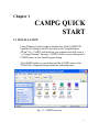


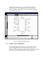
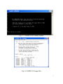


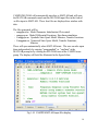
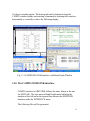

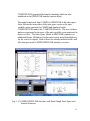
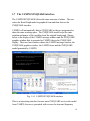


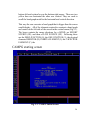
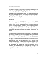


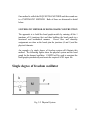


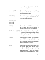

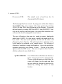

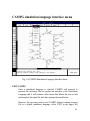


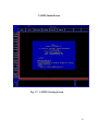
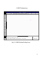


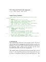
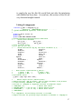
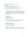


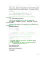

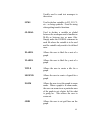
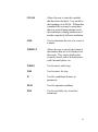


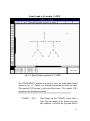

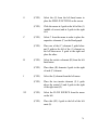


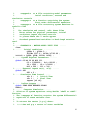

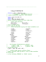

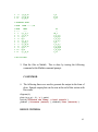


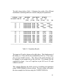


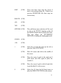
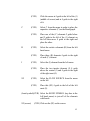


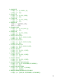
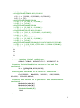

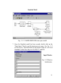
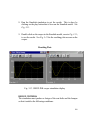


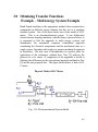
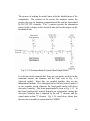
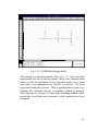


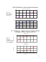
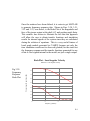
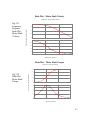
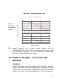

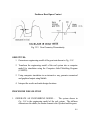
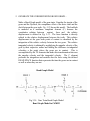
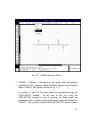


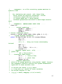
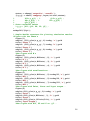

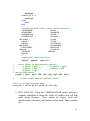

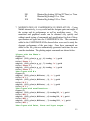
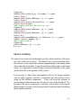
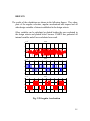

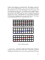

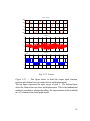


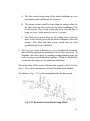
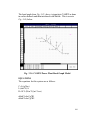

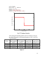

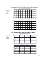
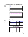
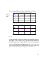

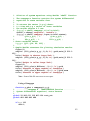
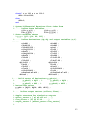

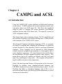


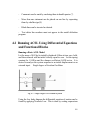


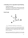


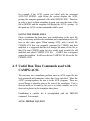


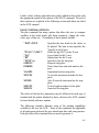
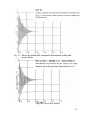
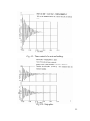


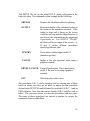
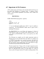

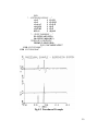

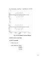


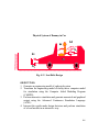
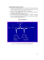


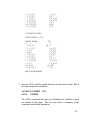


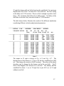
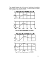
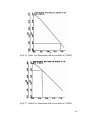
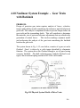
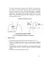
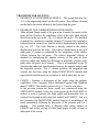


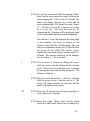

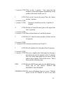

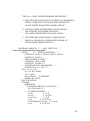
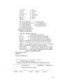
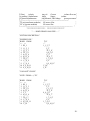


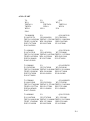
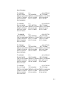


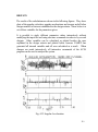
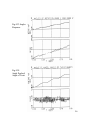

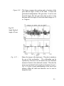
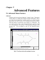
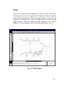
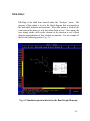
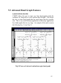
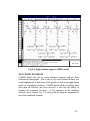
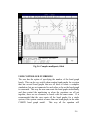
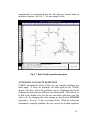
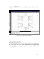
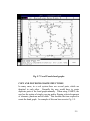
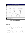
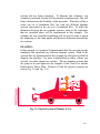
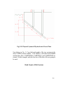
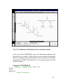
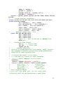

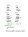


![Final Report - [Almost] Daily Photos](http://vs1.manualzilla.com/store/data/005658230_1-ad9be13b69bd4f2e15f58148160b0f22-150x150.png)