Download LSAIF-Autofluorescence Signal Removal with Maestro Software

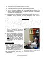
AUTOFLUORESCENCE SIGNAL REMOVAL WITH MAESTRO™ SOFTWARE
This protocol has been provided for training and educational purposes to familiarize
you with our fluorescence equipment and animal anesthesia system.
Key Points:
• Only trained LSAIF technicians are authorized to use the fluorescence equipment
and will be performing your experiment for you. Because we believe that an
educated user is a satisfied user, we are pleased to provide this detailed protocol
for your records.
• The protocol may not be identical for each imaging session, but will provide a
general overview of what you can expect.
• At any time during your imaging session, you are encouraged to ask questions and
make suggestions. Our technicians are a great resource and are here to help you.
This protocol is divided into
two
main
parts:
Animal
Preparation and Anesthesia
and Imaging the Animal. This
protocol explains the use of the
Maestro™
multi-/hyperspectral fluorescence imaging
system (Figure 1), including
animal anesthesia, collection of
images, and elimination of
autofluorescence.
The animal images in this
sample protocol were obtained
from a mouse that had a tumor
located in its lung, which was
expressing green fluorescent
protein (GFP). In this protocol,
hair
removal
is
essential
because the presence of hair
on the animal can obscure the
signal from the tumor. Hair
removal must be performed
while the animal is under
general anesthesia in the
imaging chamber (Figure 1B).
A
C
B
Figure 1. Components shown: A) Maestro™ imaging chamber, B)
induction chamber, and C) anesthesia controls.
Longwood Small Animal Imaging Facility
www.centerformolecularimaging.org
ANIMAL PREPARATION AND ANESTHESIA
1) Verify that there is sufficient O2 in the
tank to last for the duration of the
planned procedure.
C
a) Verify that the vaporizer is full by
checking the fluid level through the
site glass window (Figure 2).
b) If the vaporizer is not full, unscrew
the top of the isoflurane refill port,
and slowly add isoflurane to the
port. Close the bottle quickly and do
not inhale isoflurane vapor.
2) Check all connections and make sure
that the inflow (from the vaporizer’s
common outlet) and outflow to the
chamber are in the open position.
3) Close the flow to the nose cone in the
imaging chamber.
D
A
B
E
Figure 2. A) Gas flow control, B) Isoflurane site
glass, C) flow to imaging chamber, D) flow to
induction chamber, and E) vaporizer.
4) Place the animal inside the induction chamber and close the lid tightly.
5) Turn on the O2 source and set the fresh gas flow into the chamber at 2.5 L/min
using the flow meter control knob.
6) Turn on the vaporizer and adjust the isoflurane concentration to 2.5%.
7) When the animal is in a moderately deep plane of anesthesia (lying on its side
and breathing rhythmically), remove it from the induction chamber and close the
lid.
8) Connect the animal’s nose to the nose cone in the imaging chamber and open the
gas flow to the nose cone. If there are more animals to be studied, place the
next animal in the induction chamber. Otherwise, the valve to the induction
chamber can be closed. Because rodents are obligate nose-breathers, it is not
essential to include the mouth in the nose cone.
a) If the animal needs to be shaved, use animal clippers while the animal is in the
imaging chamber.
b) If complete hair removal is necessary, apply the depilatory while the animal is
in the imaging chamber.
9) Monitor the depth of anesthesia throughout the procedure, making sure that:
Longwood Small Animal Imaging Facility
www.centerformolecularimaging.org
a) The animal’s nose is completely inside the nose cone.
b) The animal is breathing rhythmically, but is otherwise motionless.
c) There is no reaction to a pinch test. Pinch the animal’s toe; if there is a
reaction, increase the percentage of isoflurane by 0.5%. Wait a few minutes
and repeat, until there is no reaction.
10) Control animal body temperature with Spin Systems heating mat set to 38°C.
Temperature may be monitored using rectal temperature probe from SA
instruments.
11) Begin the imaging procedure. (See Imaging the Animal section.)
12) After the imaging is complete, remove the animal and return it to its cage. The
animal should regain consciousness within 5 minutes. If the animal does not
regain consciousness, adjust the vaporizer to 0% and place the animal back into
the induction chamber. (By adjusting the vaporizer to 0%, the animal will
receive pure oxygen, which should help revive it.)
13) Shut off the isoflurane vaporizer and the O2 flow at the tank.
14) Check the flow meter to verify that the
O2 flow is off and turn the gas flow
control knob to the OFF position (fully
closed clockwise).
A
15) After all of the imaging is complete,
weigh the f/Air anesthesia absorbing
canisters. If the canister has gained 50
grams, replace it with a new canister.
(Note: Be sure to mark down the
original weight on the canister, date of
measurement, the new weight, and
your initials).
IMAGING THE ANIMAL
B
1) Turn on the main power switch at the
back of the Maestro™ Imaging Module
(Figure 4). Make sure the computer is
powered up and then double-click on the
Maestro™ software icon (Figure 4, inset)
on the desktop to start the program.
2) Be sure the shutter switch is in the
closed position.
C
Figure 4. A) Interior light controls, B) excitation light
shutter and power controls, C) excitation light filter,
and Inset) Maestro™ software icon.
Longwood Small Animal Imaging Facility
www.centerformolecularimaging.org
3) Select the appropriate filters for the fluorescence you want to detect. The
excitation filter is selected at the Illumination Module, and the emission filter is
selected below the lens inside the Imaging Module. (Refer to the filter/dye
combination chart, which is posted on the front door of the unit and is also in the
User’s Manual.)
4) Turn on the interior lights using the switches on the upper right exterior of the
Imaging Module.
5) Set the Imaging Table to the required
height for the size of your specimen (Figure
5).
A
a) Refer to the areas marked on the stage
surface, and note the number of the
appropriate rectangle engraved on the
stage surface.
b) Move the stage up or down to match the
stage height number to the number of
the appropriate rectangle on the stage
surface. The stage position is unlocked
and locked using the finger grips on the
front of the stage.
6) Manually adjust each of the Excitation Light
Arms to match the stage position. Move the
Excitation Light Arms up or down to match
their position numbers with the stage
position numbers.
7) Look on the left side of the computer
screen, and check that you are in the
Acquire mode. If not, click on the Acquire
tab at the top of the left panel.
8) Configure the settings for the type
images and the image quality desired.
B
C
D
Figure 5. A) Emission filter, B) excitation light
arms, C) anesthesia connections, and D)
imaging table adjustments.
of
a) Set the Region-of-Interest (ROI) and binning to full field (large black square)
and 2x2 binning.
b) In the Wavelength and Exposure box enter the desired wavelength, i.e., if the
desired signal is caused by GFP, and then set the wavelength to 520 nm.
9) Increasing the parameters of binning from None to 2x2 results in a 2-fold
reduction in both x and y resolution, but also in a 4-fold reduction in file size and
Longwood Small Animal Imaging Facility
www.centerformolecularimaging.org
a 4-fold enhancement in sensitivity. For most experiments using a single mouse,
2x2 binning is optimal.
10) Click the small box next to the word Live.
11) Click the box labeled AutoExpose in the block labeled Live.
12) Manually focus the camera lens to get a sharp image of your specimen.
13) Turn off the interior lights, and close the Imaging Module door.
14) Turn on the Illumination Module power
switch and open the excitation light
shutter using the switches on the right
lower exterior of the Imaging Module.
(Note: Exposure of the animal to
excitation light should be minimized to
avoid photobleaching. When imaging has
been
completed,
immediately
close
excitation shutter.)
15) Select 520 in the Wavelength (nm) tab in
the Wavelength and Exposure box. In
order to obtain the best possible image,
the live image should always show the
target peak emission wavelength (Figure
6).
16) Select an exposure time in the Exposure
(msec) tab in the Wavelength and
Exposure box.
a) If you do not see an image, increase the
exposure time by clicking the up-arrow
in the Exposure (msec) box. You may
also use the AutoExpose Cube feature to
automatically set the exposure. Either
method will derive an effective exposure
time; however, the autoexpose method
may have a few overexposed pixels at
some of the wavelengths. If you use this
method, it is important to check all the
wavelengths in range to check for
overexposed areas.
b) If the grayscale image shown on the
screen has any large areas marked with
red, this indicates that the light is too
Figure 6. Acquire Tab with Wavelength
and Exposure box.
Longwood Small Animal Imaging Facility
www.centerformolecularimaging.org
bright, and you should reduce the exposure time by clicking the down-arrow in
the Exposure box (or enter a lower number). Click Acquire Mono to take a
snapshot of the grayscale image before acquiring the cube.
17) Collect the spectral cube image, following these steps:
a) In the Cube Wavelength Selection box, select the Preset Filter Setting that
corresponds to the filters being used. If you do not find a preset that works
for your specimen, select the Manual Adjustment option and enter the settings
manually.
b) The cube is the range of wavelengths that the system moves through and
captures image data. As a result, the range should have a midpoint around the
peak emission wavelength of the target. The Maestro™ system, however, has
a total wavelength range of 500-900 nm; therefore, for GFP or high NIR Peak
emission, it is not possible to center the wavelength.
i) Select 500 in the Start (nm) wavelength.
ii) Select 720 as the End (nm) wavelength.
iii) Select 10 as the Step (nm).
iv) Select 100 as the Exposure (msec).
18) Click Acquire Cube to collect images at the selected step size over the
wavelength range selected. Click Acquire Mono to take a snapshot of the
Grayscale image before acquiring the cube.
19) When the image cube opens,
a color version of the image
will be displayed in the upper
left portion of the computer
screen (Figure 7).
20) Select File, and then Save
Cube. This will open a dialog
window asking where to save
the raw data and what to
name it. Select the images
in the correct directory and
select Save. If this is your
first visit to the Longwood
SAIF, you may need to create
a new directory for your
current
imaging
session;
then, select Save.
Figure 7. Image cube with color representation of the image.
Longwood Small Animal Imaging Facility
www.centerformolecularimaging.org
21) Select the various elements of your specimen, such as autofluorescence and
each specific fluorescence signal you expect.
a) Click the Draw button next to the blue color bar in the Spectral Library panel.
b) With the mouse, move to an area of the specimen that contains only
autofluorescence. Hold down the left mouse button, and draw a line in the
autofluorescence area.
c) The average spectrum under this line will appear in the graph area of the
analyze tab.
d) Click the Draw button next to the red color bar in the Spectral Library panel.
Move back to the image, and draw a line over the specific fluorescence signal
area.
e) The average spectrum under this line will appear in the graph area of the
analyze tab. This spectrum should appear different than the autofluorescent
signal. If the two spectrums are identical, repeat steps 21b-21d in different
areas so that the spectra are varied.
22) Extract the real fluorescence signal from the autofluorescence, as follows:
a) Select Manual Compute Spectra, which appears at the bottom of the Spectral
Processing tab and a Compute Spectrum window will appear.
b) Set the Known Spectrum color to blue, which is the autofluorescence signal.
c) Set Mixed Spectrum to red for the combination of autofluorescence and
specific fluorescence signal.
d) A new graph will appear in the bottom with the computed spectrum.
e) You can name the computed spectrum, which reflects the real fluorescence in
the text box at the bottom.
f) Set the real fluorescence to the desired color, i.e., green.
g) Examine the spectral graph. You should see less overlap between the
autofluorescence signal and the specific fluorescence signal as compared to the
autofluorescence signal and the mixed signal.
h) Click Transfer to Library.
23) Click the Unmix button appearing in the Spectral Processing tab.
Longwood Small Animal Imaging Facility
www.centerformolecularimaging.org
Figure 8. Compute Spectrum Window.
24) Several new images will appear. There will be an unmixed image for each color
with a check mark in the Spectral Library panel (Figure 8). These images will be
smaller and surrounded by a colored border corresponding to the selected
pseudocolor. The specific fluorescence signal should clearly display the area
Figure 9. A lung tumor in mouse that has been labeled with GFP before (left) and after (right) the system
has unmixed and reconstituted the image capture data. The signal is deep within the body; under normal
imaging, the autofluorescence and scatter of the tissue would almost completely obscure the true
fluorescent signal (left). Using the Maestro™ software, the true signal from the tumor can be visualized
(right).
Longwood Small Animal Imaging Facility
www.centerformolecularimaging.org
occupied by the desired fluorescence signal. These images are all scaled fro
display, so their relative brightness may not reflect relative abundances. There
will also be a larger, pseudo-colored composite image in the top right of the
main window, displayed beside the original RGB image of the specimen. The
colors used to create this image are library pseudocolors. The result should be a
clear display of the specific fluorescent signal with obvious differentiation from
the autofluorescence.
Figure 10. Save Image menu.
Figure 10. Save Image Directive
Save Image (as Displayed)
Save All Images (as Displayed)
Save Image (as Unscaled Data)
Save All Images (as Unscaled Data)
Explanation / Use when . . .
Saves top image as displayed.
Saves all images as displayed.
Saves top image with default scaling parameters.
Saves all images with default scaling parameters.
25) Save the resulting images, as follows:
a) Under the File menu (Figure 10), select Save All Images (as displayed). A file
prompt window will then appear to save each image on the screen. These
images will be saved as TIFF images. The raw unmixed images can also be
saved using the Save all Images (as unscaled data) format; this will save the
data in its raw, 16-bit format so that it may be quantified at a later time.
b) Save the Spectral Library. You can load this library in the future to unmix this
or similar cubes using the Maestro™ software.
c) Save the exposure times as reference for later tests.
26) After all images have been saved, you may select Close All Windows from the
Windows menu item.
27) To close the image cube, click the  in the upper right corner of the displayed
image, or select Close Image Cube under the File menu.
Longwood Small Animal Imaging Facility
www.centerformolecularimaging.org