Download 1 - Department of Chemistry - University of Wisconsin–Madison

University of Wisconsin–Madison
Chemistry Department
Varian NMR User's Guide
by: Charles G. Fry
(updated December 19, 2001)
Note: This guide provides an introduction to use of Varian equipment at the
UWChemMRF. This guide is not intended in any way to be a
replacement to the excellent Varian documentation! All students should
refer regularly to the Varian VNMR Liquids Users Guide for learning and
the Varian VNMR Command Reference Guide for specific guidance. All
the Varian documentation is available in both hardcopy and on-line.
Copyright © 1996-2001 Charles G. Fry
All Rights Reserved.
Table of Contents
Page i
Table of Contents
UW Chemistry Magnetic Resonance Facility (UWChemMRF).........................4
nd
I. Facility Layout (2 floor Matthews)..................................................................... 4
SGIs – NATOTH (Avance host computer) and GQUAN (for off-line data workup) ..... 5
II. Facility Personnel ................................................................................................ 5
Quick Guide for New Users................................................................................6
I. Login ................................................................................................................... 6
II. Setup................................................................................................................... 6
A. 1st Time:
6
B. Parameters:
6
C. Variable Temperature
6
III. Locking and Shimming ........................................................................................ 7
A. Sample Prep:
7
B. Locking:
7
C. Shimming:
7
IV. Probe Tuning and 1H Calibration ......................................................................... 8
V. Acquisition ........................................................................................................... 8
VI. Saving and Deleting Data, and Backups.............................................................. 9
VII. Logging Out......................................................................................................... 9
VIII.
Don’ts ........................................................................................................... 9
Introduction to Unix and VNMR .......................................................................10
I.
II.
III.
IV.
V.
VI.
Common Unix Commands................................................................................. 10
Common VNMR Commands, Parameters and Flags ........................................ 11
VNMR Directory Structure ................................................................................. 14
Common Pulse Sequence Setup in VNMR........................................................ 14
VNMR to Bruker-AM/AC Parameter Conversion Table ...................................... 16
Trouble-Shooting ............................................................................................... 20
Operation of Unity–500 .....................................................................................22
I. Proper Exiting and Logging In and Initial VNMR Setup...................................... 22
II. Commands for First Time and Novice Users ..................................................... 22
III. Probe Changes ................................................................................................. 22
Table 1. Description of Probes on Unity-500 and Inova-500
23
Table 2. Calibrations of Probes on Unity-500
24
III. Probe Tuning..................................................................................................... 24
IV. Lock and shim ................................................................................................... 25
Table 3. Field and Lock Power Settings for Unity–500
25
Table 4. Major Shim Interactions on Unity–500
26
Table 5. Shim Sensitivities on Unity–500
26
Experiments on Unity–500 ...............................................................................27
I.
Normal 1d 1H Acquisition................................................................................... 27
D. 1H pw90 Calibration
28
UWChemMRF
Table of Contents
Page ii
E. 2nd Order Shimming on a 500 MHz Spectrometer
29
F. 1d Data Workup and Plotting
29
II. X Acquisition (e.g., 31P or 13C).......................................................................... 31
Table 6. Common Decoupler Parameter Settings
32
D. 13C (X) pw90 and {1H} Decoupler Calibrations
33
III. DEPT – Distortionless Enhancement by Polarization Transfer ......................... 35
IV. INEPT – Insensitive Nuclei Enhanced by Polarization Transfer ........................ 38
V. 1d NOE-Difference Spectroscopy...................................................................... 40
VI. Homonuclear 1d Decoupling ............................................................................. 41
VII. COSY – 2d Homonuclear Correlation .............................................................. 42
E. 2d Data Workup and Plotting
43
VIII. DQ-COSY – Double-Quantum Filtered COSY (Phase-Sensitive) .............. 44
IX. TOCSY (or HOHAHA) – Total Correlation Spectroscopy................................. 46
X. Other COSY Variants ........................................................................................ 48
XI. NOESY – 2d NOE and Exchange Spectroscopy ............................................. 49
XII. ROESY – 2d NOE Spec.; Mixing via a Spinlock in the Rotating Frame ........... 51
XIII. HETCOR – 2d Heterocorrelation Spec. (“normal” X nucleus detection) ..... 53
XIV. HMQC and HSQC – 2d Heteronuclear Spectroscopy (“inverse”
experiment with 1H detection)............................................................................ 54
XV.
HMBC – 2d Long-Range Heterocorrelation Spec. (inverse detection) ....... 56
XVI. Other Heteronuclear Correlation Experiments ............................................. 57
XVII.
Fitting Partially Overlapping Peaks –
Deconvolution in VNMR
58
XIX. 1H Spin-Lattice Relaxation, T1..................................................................... 59
II. Rapid Determination of T1 by Inversion-Recovery Null Method ......................... 59
III. Quantitative measurement of T1 by Inversion Recovery Method ....................... 60
A. Comments
60
B. Acquisition Set-up
60
C. T1 Analysis (see Varian Subject manual, Adv. 1d section)
60
XIX. Cross-Polarization/Magic-Angle-Spinning NMR............................................... 62
A. Preparation of MAS spectra
64
B. Simulation of spinning sideband patterns
64
C. Least-squares fitting of spinning sideband patterns
64
Data Backups from UNIX Workstations ..........................................................66
I.
Backups to Colorado Systems Tape Drive on Windows NT Network ................ 66
A. Perpare tar file on UNIX workstations
66
B. Move file to NT server
66
C. Backup file to Colorado Systems tape drive
66
D. Recovering backup’ed up data
66
II. Backups to IOmega Zip Drive on Windows NT Network (currently installed
on Morder, Terminus, Drazi).............................................................................. 67
A. Prepare a tar file
67
B. Backup file to IOmega Zip drive
67
D. Recovering backup’ed up data
67
th
III. Backups to Pinnacle Optical Disk (on Tango on 5 floor) .................................. 67
A. Format a New Optical Disk
67
B. Create File System on New Optical Disk
68
C. Backup to Optical Disk 68
th
IV. Backups to Pinnacle CD Writer (on Twiddle on 9 floor) ................................... 68
UWChemMRF
Table of Contents
A. Transfer Data to Twiddle 68
B. Transfer Directories/Files to Easy-CD Window
Page iii
68
Administration of Varian Spectrometers ........................................................70
I.
Rebooting Sun’s on Spectrometers (requires root privileges) ............................ 70
A. Shutting down UNIX:
70
B. Powering Up UNIX:
70
Pulsed-Field Gradient Shimming With VNMR ................................................71
I. General Discussion ........................................................................................... 71
II. Normal PFG Shimming Procedure .................................................................... 72
III. First-Time Use and Detailed Explanation of Parameters ................................... 74
A. Critical Parameters
74
B. Details of Correct Parameter Setup
75
UWChemMRF
Quick Guide for New Users
Page 4
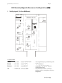
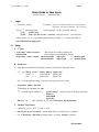
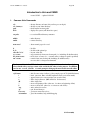
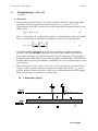
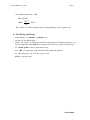
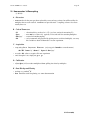
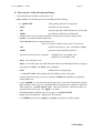
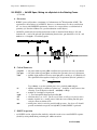
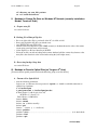
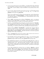
UW Chemistry Magnetic Resonance Facility (UWChemM
MRF)
I.
Facility Layout (2nd floor Matthews)
2 20 1
charlie
fry
M atthew s 2n d floor
neil
whittem ore
2 23 7
m arv
kontney
X irth
600
V ir
S S -3 00
2 20 7
S un W kstn.
2 20 9
N a rn
500
2 21 0
Vorlon
500
H o m er
300
A then a
300 a
2 22 1 d
2 22 1 c
2 23 0
N MR PCs
360
N a To th
S G I W kstn.
2 20 2
ESR
P hoe nix
250
2 22 4
2 22 1
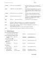
As of July, 2001
ATHENA
–
AC+ 300
routine 1H/19F/31P/13C
–
auto-sample changer, quad-nucleus probe
HOMER
–
AC+ 300
routine 1H/13C
–
1H/13C
PHOENIX –
AC+ 250
routine BB VT
–
routine BB (29Si/11B/2H/199Hg/etc.),
variable temperature
VIR
UNITY-300 solid-state NMR
–
conformational, motions, solid-state
packing, catalysts, amorphous and glassy
compounds
–
dedicated
UWChemMRF
Quick Guide for New Users
Page 5
NATOTH
–
Avance-360 non-routine BB VT
–
long-term VT, kinetics, concentration limited
samples; 5 and 10 mm BB probes, 5 mm inverse
probe
NARN
–
UNITY-500 non-routine 1H/BB VT
–
high-sensitivity, sample-limited (1H < 5 mg, 13C <
15 mg), short-run, sophisticated experiments (e.g.,
HMQC, DQCOSY, gCOSY, gNOESY); limited
access
VORLON
–
INOVA-500 inverse exps, 2D studies
–
long-term, sophisticated, gradient-enhanced
experiments; combi-chem MAS probe; limited
access
XIRTH
–
INOVA-600 long-term 2D studies
–
long-term, most sophisticated, gradient-enhanced
experiments (e.g., NOESY/ ROESY, HMQC,
DQCOSY); limited access
ESR
–
ESP-300
–
paramagnetism, free-radical chemistry
PC’s
–
–
DEATHSTAR, TERMINUS, MORDOR, VULCAN surround the main printer GKAR
KOSH has special software; BABYLON (128.104.70.61) is the Win-NT server
Sun’s
–
–
for data workup, UltraSparc 1 (M170)’s CENTAURI and ZHADUM are located in rm
2010, VORLON is in rm 2201a
NARN and SHADOW (Sparc 5’s) are hosts for the respective instruments
–
NATOTH (Avance host computer) and GQUAN (for off-line data workup)
SGIs
II.
electron spin resonance
Facility Personnel
Director, Chemistry Instrument Center
Prof. Paul M. Treichel Rm. 6359A
262-8828
[email protected]
Rm. 2128
262-3182 o
276-0100 h
[email protected]
[email protected]
Rm. 2132
262-7536 o
[email protected]
Rm. 2210
262-0563
[email protected]
Rm. 2225
262-8196
[email protected]
rm 8131
rm 7363 (Daniels)
262-7948
262-0414
[email protected]
[email protected]
Director, Magnetic Resonance Facility
Dr. Charles G. Fry
(Charlie)
Associate Director, MRF
Dr. Neil Whittemore
NMR Engineer
Marv Kontney
ESR Engineer
Roger Clausen
Teaching Assistants
Lizheng Zhang
Ekasith Somsook
UWChemMRF
Varian NMR User’s Guide
Page 6
Quick Guide for New Users
created 12/01/97 – updated 9/27/99
I.
Login
•
Username: practice
Password: [do not use 9th floor password; nothing from a
dictionary; at least one number; case sensitive]
• data to → /zhadum/practice
UNIX:
VNMR:
[other partitions: europa, ganymede, starbase]
mkdir name
FILE left-click on name CHANGE (will place data in ~practice/name)
• shims, macros, etc. to /export/home/practice/vnmrsys/shims or ~/vnmrsys/maclib, etc.
• exit VNMR before logging out!!
II.
Setup
A. 1st Time:
; this will put reasonable parameters in
• MAIN MENU SETUP 1H,CDCL3
• phasing=100
; shows complete spectrum while phasing
ngbar_plot
• MAIN MENU MORE CONFIG SELECT PLOTTER
or shadowp_plot
SELECT PRINTER
ngbar_print
or shadowp_print
B. Parameters:
•
Setup probe and pulsed-field gradient parameters using macro with probe name:
e.g.,
type bbswg produces probe= ‘bbswg’ pfgon=’nny’
bbold →
probe=’bbold’
pfgon=’nnn’
→
hcx
probe=’hcx’
pfgon=’nny’
It is critical the probe parameter is set for correct parameters to be setup.
•
MAIN MENU
1H
SETUP
Nuc,Solv
should be ok; check nt and gain
13C
probe=’bbswg’ (make sure this is the probe installed)
dmm=’w’
dmf=10000
dpwr=40
turns decoupler on (see also UWMACROS DECOUPLER ON)
– check decoupler settings, e.g.,
dm=’yyy’ su
C. Variable Temperature
•
switch to N2 gas for 20°C > temp > 40°C
•
turn VT flow up to eject samples (do not switch back to air unless close to ambient)
•
Use UWMACROS SET TEMP to change temps (or macro settemp or similar)
UWChemMRF
Quick Guide for New Users
Page 7
UWMACROS SET TEMP should be used instead of manually setting temperature; this macro
avoids inadvertant temperature changes that can otherwise occur.
•
±20° changes take 15 mins or so before probe tuning and shims will be stable.
±50° changes take ~30 mins.
±100° changes may take 1 h (should be done in steps no bigger than ±50°).
– It is the student’s responsibility to finish early enough that their VT work does not affect the
next user!!
•
hcx probe -80 to +60°C
bbswg probe -150°C to +80°C
bbold probe -150 to +150°C
h1f19 probe -150 to +150°C
III. Locking and Shimming
A. Sample Prep:
• Need ≥ 0.6ml (4 cm height) solvent for Varian probes to attain good 1H shims (without
extraordinary shimming).
• Set sample to 67 mm below bottom of spinner (use ruler), or
center in rf coil region (use Varian depth gauge) if solvent < ~5 cm high.
• On a 500, it is critical that the sample be clear (no particulate floating if possible), and the tube be
of high quality (Wilmad 506 minimum, 528 better) with no nicks or scratches. Keeping within
these standards will allow excellent quality shims to be attained in ≤ 5 min shimming. Reasonable
shims can be attained in other conditions, but with longer shimming sessions, and no guarantee
that good quality lineshapes can ever be achieved.
B. Locking:
• use UWMACROS LOADSHIMS
! or
or manually use rts!
• rts(‘hcx.shim’) loadshims
(loadshims → load=’y’ su load=’n’ su)
rts(‘bbswg.shim’) loadshims
rts(‘your-shims’) loadshims
! will save in /export/home/practice/vnmrsys/shims]
[FILES SAVE SHIMS or svs!
• in ACQI window:
set FIELD → until fid on-resonance (no oscillations) and positive
LOCK POWER (see START suggestion, but be aggressively higher if
needed)
LOCK GAIN
NOTE: IF ACQI WINDOW DOES NOT APPEAR, USE ‘ACQI’ TO CALL IT UP.
• should lock up now
• turn SPIN ON if routine 1D (not if 2D or selective 1D experiments)
C. Shimming:
• shim: LOCK PHASE → Z1 → Z2 to achieve maximum lock signal
• lower LOCK POWER (approaching FINAL suggestion; but keep lock level > 15)
UWChemMRF
Varian NMR User’s Guide
Page 8
nd
LOCK PHASE → Z1 → Z2 (2 order) → Z3 (usually not necessary)
• spinning:
nd
X → Y → XZ (2 order) → YZ → XY → X2-Y2 , then back to above
non-spinning
(2D do all without spinning)
• check shims using standard 1H setup with nt=1
set cursor on solvent singlet, nl dres ; should be ≤ 1 Hz in most cases; highly dependent on
tube; 507’s (stockroom) will sometimes need Z3+Z4 adjustments; 528’s typically should not)
IV. Probe Tuning and 1H Calibration
• Use Hewlett-Packard scope to tune probes:
–
disconnect 1H cable (with small silver barrel filter attached) from probe, and hook HP scope
into probe
–
push H1 PROBE on the scope
–
tune in TUNE capacitor (bottom) to center dip
tune in MATCH capacitor (upper) to get dip down to bottom 2-3 squares
readjust both to center and bottom dip appropriately
–
disconnect scope cable and reconnect 1H
–
tune 13C or other X nucleus if needed at this time
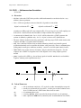
• check 1H pulsewidth using array command: use pw 30 3 3 to set up first array; check about
360° (going negative to postive as pw increases); pw90 = pw(@ 360°°) / 4
• pw90 check is required for checkout; also necessary before querying facility staff about probe
V. Acquisition
• Check that there is no external attenuation in-line for 13C or other nuclei runs.
• Set gain=40 and listen/watch for an ADC OVERFLOW beep [there is one beep for completion
of the acquisition, and a second beep if there is an ADC overflow]; turn gain down in 10 dB steps
until ok (this is recommended setup; computer sees clipping better than you will in next
example!).
• Can also perform a nt=1 acquisition, then df; if fid looks normal, type gf (wait > 2s!!!), then
can go into ACQI FID and observe fid directly while changing gain.
• go or
ga (will automatically wft) or
au (will perform additional commands useful for 2D or auto-saving data)
• 1H acquisition usually needs only a check of nt.
– movesw similar to ^O in EP on AM/AC’s
– movetof similar to changing O1 on AM/AC’s
• 13C, turn on decoupler:
dm=’yyy’ su
UWChemMRF
Quick Guide for New Users
Page 9
– remember to turn off when done!
– set nt=1e6 if don’t know needed number of scans
can wft after each bs scans (lb=2-4 needed for 13C)
use sa to stop acquisition once S/N is good enough
• cursor close to peak, nl rl(77p) will correctly reference CDCl3 peak; rl1(77p) for f1 in 2d’s
• dsx → wft dscale(-3)
• ppa pscale pl page typical plot
VI. Saving and Deleting Data, and Backups
• FILES SAVE FID or
svf(‘data-name’) ..... ; saves only raw fid but with all parameter’s intact
• MAIN MENU FILE SAVE FID
type in name without quotes
• MAIN MENU FILE left-click on data-name DELETE
will delete data
• use FTP program on PC’s and connect to ZIP’s to backup
VII. Logging Out
• exit VNMR first
• right-click on background, exit
VIII. Don’ts
• use Unity without VT regulation (run at 26°C if just want ambient)
• use too little solvent; Varian probes require more solvent than Bruker probes; too little solvent
will just give you a terrible shimming session
• run VT outside 20 to 40°C without switching over to N2 gas
• run VT below 10°C without Variac on
• run VT outside -80 to +60°C on hcx probe, -120 to +80°C on bbswg probe
UWChemMRF
Varian VNMR User’s Guide
Page 10
Introduction to Unix and VNMR
created 3/5/95 – updated 12/19/01
I.
Common Unix Commands
cd ~
cd ~/vnmrsys
pwd
df -k
–
–
–
–
! paths
– see section III on directory structures
mkdir
rmdir
– make directory
– remove directory
man cmnd
– show manual pages for cmnd
ls
ls -la
alias dir 'ls -la'
cp -r name
mv fname tname
rm -r name
–
–
–
–
–
–
change directory to home (dir you first go to on login)
change to your vnmr directory
show current location (path)
display file system (will show free space)
list files
list files with options lga
in your .cshrc file
copy recursively from name down path (i.e., including all subdirectories)
move fname to tname (i.e., a rename unless a change in path is specified)
remove from name down path (including all subdirectories)
use care; this is a dangerous command!
Use the text editor in the CDE windowed environment if possible (much easier than vi), but
always finish with a carriage return at the end of the file when creating macros. In addition,
you can use textedit filename at a unix prompt to bring up the more-usable textedit editor.
vi filename
i
a
x
dd
^
$
:wq
:q!
/text<ret>
:set number
–
–
–
–
–
–
–
–
–
–
–
edit filename using vi editor (cgf has couple pages of Vi Quick Reference)
insert (must use ESC or double up/down arrow to exit insert mode)
append; insert after cursor position (use at end of line)
delete single character (10x will delete 10 characters)
delete single line
move to beginning of line (then use i to insert at beginning of line)
move to end of line (then use a to insert at end of line)
write and end vi session
quit, discard changes
go to next occurrance of text
gives line numbers, help with debugging
UWChemMRF
Intro. to Unix and VNMR
II.
Page 11
Common VNMR Commands, Parameters and Flags
(! particularly useful commands)
! dg
dg1
dgs
– display group (normal parameters)
– display second (processing, plot... parameters)
– display shim group
! dps
da
! array
– display pulse sequence
– display array
– powerful array command, for stacked acquisition (kinetic exps, pw checks)
! full
wysiwyg=’n’
– uses full screen; needed after dssh and other commands (is NOT the same as
the DISPLAY INTERACTIVE FULL button)
– sets display so scaling does NOT match printer
svf(‘filename’)
rtf(‘filename’)
svp(‘filename’)
rtp(‘filename’)
svs(‘filename’)
rts(‘filename’)
–
–
–
–
–
–
wexp=’svf(\’filename\’)’
explib
cexp(#)
delexp(#)
save file (1d or 2d) with associated data, phasing, etc. (FILE SAVEFID)
reads file (menu alternative MAIN MENU FILE)
save only parameters (1d or 2d); significant savings in disk space!!
reads parameters
save shim settings to user directory ~/vnmrsys/shims ( FILE SAVESHIM)
reads shims (follow with loadshims macro; UWMACROS LOADSHIMS)
– saves data to filename at completion of experiment (\’ required for
quotes within the main quotes
– requires au used to start acquisition
– lists all experiment areas (menu MAIN WORKSPACE LIBRARY)
– creates experiment area number # (see also WORKSPACE)
– deletes experiment area number # (save disk space; see also WORKSPACE)
temp24
– UW macro to set temp to 24°C (cp into your ~\vnmrsys\maclib, rename and
edit for other temperatures); (UWMACROS SET TEMP)
vttype=0 or 2
– variable temp controller not present (=0) or present (=2)
temp='n'
– no temp specificied for control
vttype=0 temp='n' su – command preceeding probe change (see macro tempoff)!!
vttype=2 temp=24 su – command to re-establish temp control at 24°C after probe change (see macro
temp24)
tn='Si29'
d# (e.g., d1=1)
pw=8
p# (e.g., p2=4000)
tpwr
tpwrf
nl
! rl(-9.86p)
rl1(-9.86p)
lb=5
–
–
–
–
–
–
set transmitter to 29Si frequency (uses look-up table; see macro tuneh)
set delay time in seconds (use dps to make sure about timing)
common pulse width in µsec (use dps)
pulse width in µsec (use dps)
observe transmitter power set in dB, from 0 to 63, larger is more power
observe transmitter fine power control, from 0 to 4095, ~3db spread
–
–
–
–
first set cursor close to peak, then finds nearest line
first use nl to set cursor exactly on, then sets reference
expand about correct reference on diagonal peak, use to ref f1 axis
gives exponential broadening of 5 hertz with wft or ga
UWChemMRF
Varian NMR User’s Guide
wft
! aph
np=4k
fn=16k
lsfid=2
! movesw
Page 12
– weighted (depending on parameters set) FT
– good automatic phase to at least start phasing
– often set by sw, this directly sets to 4096 points acquired, changes aq
– number FT to, with previous command does two zero fills
– left shift two points before FT (increase if getting baseline rolling)
– macro sets sweep width sw to right and left cursor positions
cz
bc
bc(5)
– zero all integral resets (use menu button reset and mouse for resets)
– baseline correction with default spline fit; depends on integral resets
– baseline correction using 5th order polynomial fit
pl
text('text goes here')
atext(‘more text’)
pap
ppa
axis='p'
pscale(-3)
axish pscale(-6)
page
–
–
–
–
–
–
–
–
–
plot spectra(um) as displayed
text header plotted on top of page
adds lines to text header
plot all parameters
plot only a few parameters
set axis to ppm ('h' for hertz, 'k' for kilohertz)
plot scale (in current units)
macro to set Hz scale and plot axis 6 cm below spectrum
go to next page for plotting
clradd spadd
addi
s1
r1
md(3,4)
–
–
–
–
–
clear exp5 and place current spectrum in exp5 (setup for addi)
add/sub (dual display-like) routine
save display parameters (can use s1 through s9)
recall display 1 and display as previously saved with s1
move saved display regions (s1 to s9) from exp3 to exp4
dssh
full
dss
– display stack horizontally
– return display of one spectrum to full width
– display stack using v0 and h0 as vertical and horizontal offsets
! UWChemMRF macros
tuneh
tunesi
tunec
– tn='H1' gain=0 su ......................................... (use UWMACROS TUNE H1)
– tn='Si29' gain=0 su.....................................(use UWMACROS TUNE SI29)
– tn='C13' gain=0 su
loadshims
– load='y' su load='n' ..........................................(UWMACROS LOADSHIMS)
axisp
axish
dsx
invert
–
–
–
–
tempoff
– vttype=0 temp='n' su ......................crucial command before probe change
axis='p'
axis=’h’
wft dscale(-3)
rp=rp+180 inverts the 0-order phase of a spectrum
UWChemMRF
Quick Guide for New Users
temp24
settemp
Page 13
– vttype=2 temp=24 su vttype=0 su................................. model temp macro
– vttype=2 temp=x su [wait] vttype=0 su
! intnorm
– normalizes peak to user specified value (e.g., methyl peak to 3)
! disp2d
pconpos
pconneg
– sets up wp sc nicely for 2d plots
– plots contours of 2D spectra with positive peaks getting 10 contours, negative
peaks getting just 1
– opposite of pconpos
lpforward
– sets up for forward linear prediction
UWChemMRF
Intro. to Unix and VNMR
Page 14
III. VNMR Directory Structure
There is a user vnmrsys area and a system vnmr area. All files are looked for in user area first; if
not found there, then the system area is checked.
cd ~
move to home account for computer working at
cd /vorlon/fry
moves to /export/home/fry on vorlon workstation
rtf(‘datafile’)
reads data (fid) file; datafile name must have .fid as suffix (vnmr always
appends as such with svf command)
all datafile.fid files are actually directories containing:
/export/home/username
fid ................................................................................ actual fid data
log ............................................log file shows times for acquisitions
procpar ........................................................... processing parameters
text .................................... a text file created by command text(‘...’)
rtp(‘parfile’)
reads parameter file; parfile name must have .par as suffix (vnmr always
appends as such with svp command)
all parfile.par files have only procpar and text files
~/vnmrsys
/exp1
/maclib
/manual
/menulib
/psglib
/seqlib
/shapelib
/shims
data acquisition area; can go up to exp9, but can take significant disk space
user macro library
user manual (help for pulse sequences) directory
user menu definitions directory
user created or modified pulse sequences
user compiled pulse sequences
user created RF and gradient shapes (e.g., for NOESY1D)
user stored shim files
/maclib
/manual
/menulib
/psglib
/seqlib
/shapelib
/shims
system macro library
system manual (help for pulse sequences) directory
system menu definitions directory
system pulse sequences
system compiled pulse sequences
system stored RF and gradient shapes (e.g., for NOESY1D)
system (facility) stored shim files
/vnmr
IV. Common Pulse Sequence Setup in VNMR
[this section is directed at students wanting to know details of the vnmr psg setups]
1. Always start by reading in standard parameters using MAINMENU SETUP
UWChemMRF
Quick Guide for New Users
Page 15
2. Then continue by running a macro (e.g., cosy runs the cosy macro in /vnmr/maclib) or use
SETUP SEQUENCE COSY (reads in the same macro).
3. The better macros read in only the parameters specified in psgset macro statements within the
primary macro routine (only ProteinPack macro do not, and use rtp instead). Typically the
parameter file found in /vnmr/parlib has the same name as the macro, but not always:
e.g.
macro hmqc has statement
psgset(‘hmqc13c’,dg,dg1,pwx,pwxlvl,dpwr,...)
which reads the specified parameters in from /vnmr/parlib/hmqc13c. Reading in dg and dg1
setup the appearance of the parameter display in the dg and dg1 screens.
4. The macros for 2d sequences call another macro set2d that sets up np fn ni fn1 based on the
desired digital resolution: e.g., set2d(‘dqcosy’,3,6) sets up 3 Hz/pt in F2 and 6 Hz/pt in F1.
5. Usually, but not always set2d sets the actual pulse sequence used: e.g., inside set2d is a
statment seqfil=$1 where $1 is the first parameter passed into the macro (i.e. in this case, the
sequence name). seqfil is the compiled pulse sequence (psg) residing in /vnmr/seqlib.
6. The pulse sequence source C code resides in /vnmr/psglib. The source code is compiled with
the statement seqgen (e.g., for cosy seqgen relayh.c). Only users and vnmr1 can compile
source code, so common code must be placed in the user’s vnmrsys/psglib and compiled. The
compiled code is automatically placed into the user’s vnmrsys/seqlib which must then be copied
into /vnmr/seqlib and have the owner set to vnmr1:nmr (e.g., chown vnmr1:nmr
/vnmr/seqlib/relayh ; root permission is required for the copy and chown unless the user is
vnmr1.
7. When writing or editing a pulse sequence, it is easiest to begin with a premade parameter set.
New parameters must be created with the create(parameter<,type<,tree>>) command. See
section 5.2 in the Pulse Programming manual. It is important to correct define the parameter
when creating it: e.g., when making a new variable dpw2d for a decoupler power setting that
should not go above 35 to prevent probe damage, use the command create(‘dpw2d’,’integer’)
and follow that with setlimit(‘dpw2d’,35,0,1). Note that pulse length parameters should be
defined with create(‘pwsl’,’pulse’) to insure the units for the pulse are in µs. See the create
command information in the vnmr documentation for other parameter types.
8. Some newer sequences being written at Varian usually now use a phase table named the same as
the sequence and located in /vnmr/tablib, although the newest sequences avoid the use of tablib
by specifying the table within the pulse sequence itself (rather than externally).
9. Typically the macro finishes by setting some parameters directly, and then displaying the help
file for the sequence that resides in /vnmr/manual via the command man(‘relayh’) as and
example for cosy.
10. Keep in mind that all vnmr usage looks for macros, parameters, pulse sequences, etc. in the
userlib (~/vnmrsys) first, and uses that copy if it exists, prior to looking in the system area
(/vnmr). Thus, every user can have their own version (not recommended!) of the same sequence.
User’s are encouraged to copy a sequence into a new name in their own directory. Finally, I am
beginning to implement an intermediate area for facility-developed software, e.g.,
maclibpath=’/vnmr/maclib.path’ . VNMR will look first at ~/vnmrsys, then at
/vnmr/maclib.path, and last /vnmr for a macro. I will update documentation here when this
implmentation is done.
UWChemMRF
Varian VNMR User’s Guide
Page 16
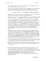
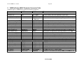
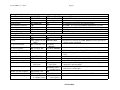
V. VNMR to Bruker-AM/AC Parameter Conversion Table
[comments apply to VNMR unless specifically mentioned otherwise]
Parameter
Experiments
standard 1d 1H
homonuclear decoupling
1d NOE difference
standard 1d decoupled X/13C
NOE-enhanced coupled 13C
quantitative decoupled 13C
DEPT 13C editing
homonuclear correlation 2d
long-range cosy
double quantum cosy
phase sensitive noesy
phase sensitive roesy
total correlation/WOHAHA
heteronuclear correlation
inverse hetero correlation
multiple bond hetero correl.
Read and Save Commands
read data file
save data file
read parameter file
save parameter file
read shim file
save shim file
load shim file
AM/AC
VNMR
Comments
ZG
go zeros memory, and starts acquisition; seqfil=’s2pul’
set the cursor on the peak and use sd to get the decoupler frequency
array can be used to run multiple decoupler frequencies in one exp.
???
???
go / s2pul
s2pul homo=’y’
s2pul homo=’y’
dm=’yyn’
s2pul dm=’yyy’
s2pul dm=’yyn’
s2pul dm=’nny’
dept
cosy
cosy tau≠
≠0
dqfcosy
noesy
roesy
tocsy
hetcor
hmqc
hmqc bond≠
≠0
RE filen.ame
WR filen.ame
RJ filen.ame
WJ filen.ame
RSH filen.ame
WSH filen.ame
none needed
rt(‘filename’)
svf(‘filename’)
rtp(‘filename’)
svp(‘filename’)
rts(‘filename’)
svs(‘filename’)
loadshims
HOMODEC.AU
NOEDIFF.AU
CPD ZG
GATEDEC.AU
INVGATE.AU
DEPT.AU
COSY.AU
COSYLR.AU
DQCOSY.AU
NOESYPH.AU
ROESYPH.AU
???
XHCORR.AU
DEPT is
preferred unless you need quat’s
X nucleus T1’s can be quite long, so this experiment can be arduous
sw/(ni*2) gives usable digital resolution; usually need ≤ 6 Hz/pt
complete phase cycling is crucial for the dq filter; nt = muliple of 8
flat baselines are important for observing small noe’s; use calfa
flat baselines are important for observing small noe’s; use calfa
useful for mixtures or separated spin systems
use only if need very high 13C resolution
important experiment for observing through linkage bonding
in VNMR, use also MAIN MENU FILE click on filename and LOAD
in VNMR, no menu selections for this
in VNMR, will search ~/vnmrsys/shims and /vnmr/shims paths
in VNMR, will save to ~/vnmrsys/shims
loadshims is UW-written macro having load=’y’ su load=’n’ su
UWChemMRF
Varian NMR User’s Guide
1d Acquisition Commands
tune 1H observe
tune 13C channel
zero and go
automation run
halt acquisition with data
resume acquisition
abort acquisition
automation setup
1d Acquisition Parameters
sweep width
center or offset frequency
solvent
Page 17
RJ H1.SET
RJ C13.SET
ZG
AU autom.nam
^H
GO
^E or ^K
AS auton.ame
UWmacro TuneH1
UWmacro TuneC13
go or ga
au
sa
ra
aa
none (try dps )
sw
tof
solvent=’cdcl3’
set spectrum window
SW
O1
none (change O1 thru
jobfile)
EP set window ^O
set offset frequency
relaxation delay
common pulse width
EP set cursor O1
RD or D1
PW
acquisition time
dwell time
# of transients to acquire
receiver gain
AQ (=TD*DW)
DW (=1/(2*SW)
NS
RG (larger # →
larger gain)
none
observe transmitter power
number of points acquired
temperature
decoupler transmitter power
TD (usually = SI)
TE
DP<ret>20H (lower
# → higher power)
set cursors
movesw
set cursor movetof
d1
pw
aq (=np/sw)
= 1/sw
nt
gain (larger # →
larger gain)
tpwr=52 (higher #
→ higher power)
np
temp=24
dpwr=40 (lower #
→ lower power)
tuneh is a UW-written macro
tunec is a UW-written macro
ga will automatically apply a wft after acquisition
all VNMR programs run from compiled routines
in VNMR, svf can be issued during acquisition to save data
seems to work only for 1d; vnmr’s ra follows an sa that stops acq.
data is lost
in VNMR, only parameters used in experiment will be shown
with solvent set correctly in VNMR, tof=0 will center spectrum for
normal organic compounds
AM/AC delay differs depending on ZG or AU to run experiment
90° length fixed by probe on AM/AC’s; depends also on tpwr on
Unity
Bruker acquires complex pairs sequentially, vnmr simultaneously
Bruker NS -1 which goes continuously → vnmr nt=1e6
on Unity, if gain=0 still clips (get ADC OVERFLOW message), insert
attenuator at preamp output
AM/AC’s observe power is fixed; Unity’s have linear amplifiers on
both observe and decouple
see temp24 and similar macros (written at UW)
vnmr parameters are logical
UWChemMRF
Intro. to Unix and VNMR
Page 18
1d Processing Commands and Parameters
fourier transform
FT
number of points FT’d
SI
line broadening parameter
LB
interactively set weighting
none
parameters
apply exponential line broad. EF
set reference
EP set cursor G
ft
fn
lb
wtia
automatic phasing
AZPK??
wft
set cursor nl
rl(0p)
aph
baseline correction
normalized intensities
absolute intensities
1d Plotting Commands
plot spectrum
plot parameters
plot axis
plot coordinates
plot size
plot integrals
plot peak picks
EP K
AI<ret>0
AI<ret>1
bs(5)
nm
ai
PX
in DPO setup
in DPO setup
X0, Y0
CX, CY
PXD???
in DPO setup
pl
ppa or pap
pscale
sc, vp
wc, vs
pirn
dll or ppf
new page
NP
page
zerio-filling occurs here (e.g., np=1024, fn=2048 will zero-fill once)
in vnmr, middle button still control intensity in all windows; left
button sets parameter
in vnmr, wft applies whatever weighting function is setup
vnmr gives example for TMS
in vnmr, lp should ~ 0, otherwise advise calfa command and/or backlinear prediction
in vnmr, bs is not recommended (default spline fit)
in vnmr, vs=100 will fill screen
in vnmr, axis=’p’ sets axis to ppm
sc is mm from right side, vp is mm vertically up from bottom
wc is mm width of chart, vs is vertical scale
printon dll printoff prints table to separate page (do before any
plotting commands); ppf plots on spectrum
UWChemMRF
Varian NMR User’s Guide
Page 19
2d Acquisition Parameters
sweep width for F1
SW1
sw1
# increments/experiments
type of 2d acquisition
IN
MC2
ni
phase
2d setup
ST2D
total time of experiment
none
interleaved acquisition
depends on routine
2d Processing Commands and Parameters
FT size in F1
SI1
reference in F1
SR1
FT and weight full set
XFB
FT and weight t2 dimension
XF1
interactive weighting
none
display color map
2d Plotting Commands
plot contours
plot size
Plot 2d using high res 1d
peak picking and volumes
none
time
il=’y’
fn1
set cursor, rl1(0p)
wft2da
wft1da
wtia
EP2D or AP2D
dconi
CPL
CX, CY
pcon
wc, wc2
plot2dhr
ll2d
none
AC/AM SW1 is 1/2 of observed sweep width; vnmr sw1 = observed
sweep width
in vnmr, phase determines total # experiment = 1× or 2×ni
AC/AM: only absolute value and TPPI are available in software
→ phase=0
vnmr: absolute value
States-Habercorn → phase=1,2
→ phase=3
TPPI
in vnmr, type in sequence macro then dps
in vnmr, acquire bs scans per increment, loop until nt completed
AC/AM square requires SI1=SI/2=SI2/2
in vnmr, for absolute value sets use do2d or wft2d
counter-intuitive commands, but mean 1st transform
can be done on t2 fid, e.g., wft(1) wtia, and on t1 fid, e.g., wft1da
TRACE wtia
in vnmr, see also pconpos and pconneg, UW written macros
in vnmr, sc still controls distance in mm from right-hand side
have 1d high res already worked up in separate exp, follow prompts
UWChemMRF
Intro. to Unix and VNMR
Page 20
VI. Trouble-Shooting
•
wrong parameters
– make sure probe parameter matches probe in magnet
•
sample won’t spin
– if probe has been changed, find TA to try reseating spin collar tube: at
top of magnet, push down the aluminum tube guiding sample in
– check that tube is not inserted too far into spin collar
– check that VT air is not turned up too high
•
sample won’t eject
– try turning the VT air up to ~ 80 (turn it back down after inserting)
– check that VT air is hooked up (rather than N2 gas which has lower
pressure)
– check that air pressure (gauge in southeast corner) is turned up to mark
•
sample won’t shim
– read in proper shim file (use UWMACROS LOADSHIMS)
– check that you have enough solvent (≥0.6 ml) and are 68mm down or
centered in rf region
– check that lock power is not too high, and that lock phase is correctly
adjusted
– let magnet warm for quite a while (up to 1h) after a cold experiment;
shims are more sensitive to this than on AM-500;
– if previous student didn’t stop early enough, you will need to adjust
especially the lock phase fairly often during the warmup (and wack the
previous person as hard as possible with a wet noodle!), and also
reshim somewhat over 30 min to 1 hour
•
command doesn’t work
– type return and try it again; some mistypes carry over to next line
•
S/N seems poor
– most likely, an attenuator has been left in line at the output of the
preamp leading back to the ADC; if your sample is not very
concentrated, remove this attenuator and adjust the gain setting
– check pw90 (at least on the observe side); if unusually long, check
with TA or facility staff
•
spectrum on screen is only an inch long or so
– type full to reset plot window (needed after dssh command)
•
says exp locked
– enter the command unlock(#) where # is the exp number that’s
locked
•
won’t let jexp#
– probably have not created the experiment (see WORKSPACE)
explib
cexp(#)
delexp(#)
•
will list all experiment areas
will create experiment area #
will delete experiment area # (saves disk space)
cannot get good pw90 calibration
– check that probe is properly tuned
– check that tpwr is set correctly (or pwxlvl for decoupler calibration)
– check that external attenuator is not placed in 1H observe position
UWChemMRF
Varian NMR User’s Guide
•
Page 21
waits a long time before acquisition starts – have one of the following flags set
spin ≠ 0
if spin is set to a number, the spectrometer will “regulate” the spinning, taking
time before acquisition to make sure the spinning is regulated
gain=’n’
for this setting, spectrometer will perform an autogain; recommend setting the
gain to a specific value manually and not using autogain
wshim=’a’
autoshimming will occur; should not be used except possibly between kinetic
runs (simply too inefficient and wastes spectrometer time)
use the flagsoff macro to set all these flags to appropriate values
•
No acqi window
Type acqi in vnmr command line
•
Can’t Connect to spectrometer
Pressing connect button on acqi doesn’t work; check that magnet leg is set to observe (not tune).
Try in UNIX terminal window: su acqproc twice (once to kill, once to restart); this should
re-enable connect to acqi
•
FIFO Underflow Error: ...Check sweep width; an excessive sweep width (>80,000 Hz) can show
this error, try reducing sw and re-acquiring.
UWChemMRF
Operation of Unity 500
Page 22
Operation of Unity–500
created 11/7/95 – updated 10/16/98
I.
•
•
•
II.
Proper Exiting and Logging In and Initial VNMR Setup
if an experiment is running, and your time is clearly in effect, use:
svf(‘savename’)
while experiment is running–will save last bs dataset
use FileManager to check that file wrote correctly (unix command df better)
exit vnmrx, right-click-and-hold on background and release on EXIT to exit CDE
do not save the workspace while VNMRX is open
Commands for First Time and Novice Users
Some of the following commands/procedures may have to be performed when first starting; many of
them will not be needed again (or only occasionally):
•
phasing=100 (or =60 on a Sparc1 if the data is >64k)
•
cexp(2) cexp(3) ...
•
click MAIN MENU MORE CONFIG PRINTER
Shadowp_LJ (laserjet portrait printing)
•
create additional experiment areas (see also MAIN WORKSPACE CREATE)
and keep clicking PRINTER until set to
–
repeat above except for
gf
following correct setup to give good fid/spectrum shimming inside ACQI FID window
PLOTTER
and click unter set to Shadowp_LJR (landscape plotting)
III. Probe Changes
ONLY FOR TA’S AND FEW STUDENTS OK’ED FOR PROBE CHANGES
•
•
•
•
•
•
•
•
•
•
•
•
•
see Table 1 on the next page for a description of probes
make sure acquisition is complete and data saved by previous user
stop temperature control by using macro tempoff (in /vnmr/maclib)
physically switch the temp controller off
eject sample (type eject at command prompt, or click eject inside shimming/acqi window);
type insert to turn the air back off
disconnect rf cabling, VT line, and probe cooling tygon
disconnect temp/heating cable using blue nonmagnetic screwdriver
unscrew two probe thumbscrews and guide probe out
insert correct probe; use care with last 1" — you may have reseat aluminum bore tube by pushing
gently downward pressure at top of magnet (necessary if sample won't spin)
reconnect cables: keep Nalorac cable and filters separate and use only for that probe
power up and restart temp control with UWMACROS SET TEMP or macro similar to temp24
read in new shims and load, e.g.:
rts('triple') loadshims (better use UWMACROS LOADSHIMS)
change probe and pfg settings appropriate for probe:
probe=’hcx’
pfgon=’nny’
probe=’bbold’
pfgon=’nnn’
probe=’1h19f’
pfgon=’nnn’
probe=’3mm’
pfgon=’nny’ (UNITY)
pfgon=’yyy’ (INOVA)
UWChemMRF
Varian VNMR User’s Guide
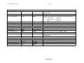
Table 1. Description of Probes on Unity-500 and Inova-500
Use the following general rules for probe selection:
• concentration limited samples: use the largest diameter probe appropriate to the experiment
– hcx or 1H/19F best for 1d or homonuclear 1H experiments
• quantity limited samples: use the smallest diameter probe appropriate to the experiment
– Nalorac 3mm probe best for all 1H experiments in this case
– strongly consider using susceptibility-matched inserts for 3mm 1H or 5mm X
experiments ( ~3×
× saving in amount of material needed to obtain a particular S/N in
a fixed amount of time, or ~10×
× decrease in time for fixed amount of material!!)
Name
Type
Temp
Description
hcx
5mm 1H {13C, X}
≥ -80°C
≤ +60°C
bbold
5mm broadband
≥ -150°C
≤ 150°C
•
•
•
•
bbswg
h1f19
nal3mm
5mm broadband switchable
(i.e. 1H observe) with pfg
5mm 1H/19F
3mm nalorac (INOVA
only)
•
≥ -130°C
≤ +60°C
•
≥ -150°C
≤ 150°C
•
≥ -40°C
≤ 40°C
•
•
•
•
invx
5mm inverse broadband
≥ -150°C
≤ 150°C
•
•
•
triple
5mm triple
≥ -100°C
≤ 100°C
•
•
•
•
inverse triple with PFG
good for 1H and 1H-X heterocorrelation
excellent 1H S/N~800
standard probe for direct 13C, 31P, 29Si, ...
observation
1H signal-to-noise (S/N) and line shape are
poor with this probe
standard probe for direct 13C, 31P, 29Si, ...
observation
1H S/N is adequate with this probe, so
probe switching for 1H observation is not
needed (for best 1H S/N, use inverse or
h1f19 probe; bbswg 1H S/N~350)
for best sensitivity 1H work when
concentration is limited
1H S/N is good (540 on EB)
for 1H 1D and 2D heterocorrelation
(13C/15N only) when sample amount is
limited, or need best water suppression
1H S/N is very good (5mm probes are
better for concentration limited samples)
for 2D hetercorrelation work: HMQC,
HMBC, HSQC
1H signal-to-noise is very good with this
probe
X S/N is poor with this probe; do not do
13C observe with this probe
for 2D 1H–13C–15N work: HMQC,
HMBC, HSQC
1H S/N is very good
13C and 15N S/N is poor
VT range is limited: -50 to +80°C
UWChemMRF
Operation of Unity 500
Page 24
Table 2. Calibrations of Probes on Unity-500
Use the following guidelines for probe calibrations:
–
short runs use facility numbers (see /vnmr/shims/probes* file for up-to-date numbers)
1H pw90 checks are always recommended time permitting for all experiments
–
–
if probe problems are suspected, check pw90’s of X and 1H observe (not decouple)
–
always perform calibrations (at minimum 1H pw90 check) for overnight or longer runs for
PT-type experiments;
–
for standard decoupling, calibrations are rarely needed even for long runs (although having
pw ~< 90° is best)
See file on-line
•
/narn/vnmr5.3b/shims/probes* .................................. if not logged onto narn
/export/home/vnmr/shims/probes* ................................. if logged onto narn
(preferable to the following is UWMACROS LOADSHIMS or FILES DATA SHOWSHIMS)
shim files that are available can be listed by entering the following commands in a UNIX window:
–
–
–
•
facility shim files:
your shim files:
user shim files:
type dir /vnmr/shims
type dir ~/vnmrsys/shims
type dir /home/user/vnmrsys/shims
or simply go to path in the FileManager
load shims with UWMACROS LOADSHIMS
III. Probe Tuning
• recommended method: UWMACROS TUNE PROBE ...
or enter macro similar to tuneh (in /vnmr/maclib)
– gain=0 is necessary for tuning (UWmacros restore original gain setting)
– make sure decoupler is off (dm=’n’ su if necessary)
• move cable (e.g., 1H) from obs or dec BNC to tune BNC
• switch knob from obs to tune
• adjust tune and match to achieve 0 on meter (in most cases, getting needle < 10 is sufficient)
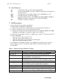
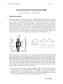
On many of the probes, there will be three capacitors:
It is essential that the two similar capacitors stay at nearly the same capacitance (i.e., same
number of turns from end), so make sure to move them together
For example, on the bbold probe, the 1H channel has a gold and two silver rods (all small diameter)
connected to capacitors. The silver are both “match” capacitors, and must therefore be turned
together: if you move one clockwise by ¼ turn, the other should also be turned clkwise ¼ turn.
•
•
•
switch knob back to obs
move cable back to obs or dec BNC
tune other channels as needed
inverse 1H/X probe: for 1H channel, tune the gold (match) and silver (tune1) knobs first, then make
sure black knob (tune2) is within ¼ turn of silver knob
UWChemMRF
Operation of Unity 500
Page 25
IV. Lock and shim
Use care when clicking on CONNECT on the acquisition window; fast clicking can crash the
computer (requiring up to 30 min to correctly reboot!), so use patience when going to acqi
•
•
•
•
•
•
•
•
click into the LOCK panel in the acqi window and turn off the lock
change Z0 until there is no oscillation in the lock signal: do not hesitate to turn up lock power and
lock gain achieve lock, but lower LOCK POWER as soon as possible to avoid lock saturation
set the LOCK POWER to recommended settings (only go up to potentially safe setting if shims are
poor; set back once shims have improved) and use LOCK GAIN thereafter to adjust amplitude
adjust LOCK PHASE analogous to a shim to get positive going signal
turn on LOCK
adjust LOCK PHASE as a shim to maximize lock signal (make sure to return to LOCK PHASE fairly
often when shimming, especially after large changes in Z2)
click into SHIM window and shim normally
– start by 1st order shimming Z and Z2; when finished take nt=1 acquisition to check line shapes
use nl dres or if S/N is excellent use nl res to get indication of line shape
– target 50% full linewidth ≤ 1 Hz for most samples, spinning or non-spinning
– now 2nd order shim Z2 (choose a direction to move Z2; this will decrease lock signal [1st order
shim had lock signal maximized at current Z2]; see if Z1 improves; if so continue, if not go other
direction in Z2)
– shim X Y XZ XY XY X2-Y2 all 1st order, then repeat 2nd order Z Z2 shim
– check line shape; if not at target try spinning sample; if improves considerably turn spin off and
work on X Y shims; if did not improve much with spinning then need to target higher order Z’s
Table 4 shows shims dependencies for the Unity-500; 2nd order shimming is required on all 500
MHz instruments (i.e., you simply cannot expect to get a good shim without it)
Table 3. Field and Lock Power Settings for Unity–500
1H
Z0 (field as
of 97/12/01)
solvent
δ (ppm)
1.93(5)
1350
acetonitrile-d3
2.04(5)
1200
acetone-d6
2.49(5)
750
dimethysulfoxide-d6
4.63(DSS)
-2000
deuterium oxide-d2
5.32(3)
-2700
methylene chloride-d2
7.15(br)
-4900
benzene-d6
7.24(1)
-5000
chloroform-d3
! Z0 will change by ~ +100 units each week.
FINAL
STARTING
lock power
10
12
14
28
15
18
25
lock power
20
20
24
40
25
30
35
UWChemMRF
Varian NMR User’s Guide
Page 26
Table 4. Major Shim Interactions on Unity–500
[+ means shim move in same direction—positive change in Z4 results in positive change in Z2]
Much of the table is not completed; since new shims installed, most interactions are now much
weaker.
Adjusted
shim
Z5
Z4
Z3
Z2
Stong
interaction
?
Z3
Z2
?
Z
Z
-
Weak
interaction
?
Z4
?
Z3
2
Z
?
Adjusted
shim
Stong
interaction
X
Y
ZX
ZY
XY
XZ
YZ
Z2X
Z2Y
X2Y2
Weak
interaction
Z
Z
Z, X3
Z, Y3, ZXY
Table 5. Shim Sensitivities on Unity–500
[number following shim is normal adjustment when shim fairly close to correct]
Sensitive
Z
Z2
Y
YZ
16 to 4
16 to 4
16 to 4
16
Z3
Z4
X
XZ
Moderate
64 to 16
XY
64
16
16
Z2X
Z2Y
ZXY
Insensitive
64
64
64
64
X3
Y3
ZX2Y2
64
64
64
UWChemMRF
Varian VNMR User’s Guide
Page 27
Experiments on Unity–500
created 5/04/97 – updated 12/21/97
I.
Normal 1d 1H Acquisition
(21-Dec-97)
A. Discussion
• 1d 1H acquisition on the Unity is simplified by the solvent=’solventname’ command. When set
appropriately, tof=0 should center the transmitter correctly.
• With identical transmitter and decouple channels, it is simple to decouple X nuclei on the Unity500 while observing 1H; e.g., for 31P set dn=’P31’ and other parameters correctly (see later
section).
• calfa is an important baseline flattening (timing correction) macro on the Unity when setting up
2d experiments. Note the use of this command in the acquisition section.
• Spin-lattice relaxation (T1) can be measured/estimated with this sequence: set p1=2*pw90
pw=pw90 and d2 appropriately (both p1 and d2 are normally are set =0; see later section for
details on T1 estimates).
• Note that Varian sequences commonly ‘hide’ some delays. In this sequence, a delay rof1 prior
to, and delays rof2 and alfa following pw are not shown. See Varian’s documentation on
pulse programming for more details.
B. Critical Parameters
d1
– relaxation delay; assuming pw~30° d1>T1 to obtain quantitative integrations
aq
– acquisition time → determines (ignoring sample effects) resolution ~ 1/aq
pw & twpr – critical for pw90 calibration and many other experiments
C. 1d 1H Acquisition
• to setup parameters (method b is recommended)
a) either read in a data file (rt or FILE left-click LOAD) or parameter file (rtp) for normal 1H
acquisition, or
! b) click on MAIN MENU, SETUP, and select nucleus and solvent
UWChemMRF
Experiments - 1H 1d Acquisition
Page 28
c) alternatively, run s2pul macro (but normally will need to reset spin=’n’, gain=0; check temp
and vttype, and check tpwr (=58 typically) and pw (=5-8µs typically).
• use UWMACRO TUNE PROBE and tune probe
• use go to start acquisition
– ga will automatically apply a wft (weighted Fourier transform) following acquisition
– use wft to manually transform
– dscale will display the axis
– dsx will apply wft dscale(-3)
• optimize sw by setting right-click or -drag (right mouse button) and left-drag (left mouse button)
cursors, and use movesw
• set reference by placing cursor close to peak, then type nl and rl command, e.g., rl(7.24p)
• if always getting ADC OVERLOAD beep, then receiver gain is too high; gain can be set three ways
(number 1 recommended):
! 1. – simply lower gain until ADC OVERLOAD warning goes away; if warning stays with
gain=0, insert attenuators into bottom BNC (preamp output), not into the probe
connections
– make sure gain is within 10B of overload warning
2. – reduce nt=1 and enter gf ; make sure to wait a few seconds (menu will flash) before
– click on acqi and then FID; make sure SPECTRUM is not selected and click on DOWN
until you see the red horizontal lines that indicate the ADC clipping limits; adjust gain
until the fid fills ~1/2 of the region to the clipping voltage
– switch nt back to original value
3. set gain=’n’ which will implement autogain adjustment (not recommended, especially for 2d
where huge artifacts can result)
D. 1H pw90 Calibration
• normally can perform calibration on sample; best to not perform it on a clean solvent since T1 for
solvents can be very long
• set tpwr to desired setting; typically 58 for 5mm probes, 52 for 3mm probes
• set d1=5-10s depending on sample T1 (d1=5 is usually ok)
! recommended: perform a coarse check of pulse widths using:
array<ret>
variable to array: pw
number of increments: 20
starting value: 3
size of increment: 3
• set nt=1 and use go; should see a sinusoidal response; if not, usually d1 needs to be longer
• to obtain an accurate pw90, check about the 360° value with an array increment size of 0.5 to 1 µs
• plot arrayed spectra using the following commands:
wft dssh
; transforms all spectra and displays in a horizontal stack
full
; resets plot area to full screen
UWChemMRF
Varian NMR User’s Guide
Page 29
E. 2nd Order Shimming on a 500 MHz Spectrometer
• Make sure the lock is not saturating. Check by watching that the lock level increases consistently
with increasing LOCK POWER. Once the lock level drops or stays steady with increasing power,
back off the power by roughly 20%. I’ve heard some Varian chemists look for a 50% decrease
when dropping LOCK POWER by 6 dB when LOCK POWER is ok (i.e. low enough to not be
saturating), but I’ve not seen consistent results doing this. I simply look for a “bounce” in the lock
level, and go 20% below the setting at which the bounce is last observed (can be difficult for fastrelaxing solvents like D2O).
• Adjust LOCK GAIN to give lock level in 25-65 range. Optimize lock level using LOCK PHASE.
Optimize lock level with Z and Z2.
• Change Z2 in one direction enough to change lock level by 5-10% (since optimized in previous
step, level will decrease). Re-optimize lock level again with Z. If newly optimized lock level is
lower than the previous one, try changing Z2 in the other direction; otherwise continue changing
Z2 in same direction until re-optimization does not improve the lock level.
• Keep changing Z2 in the same direction and optimizing lock level with Z, until an overall
maximum has been found. Set Z and Z2 to this maximum setting.
• Keep lock signal value between 25-65 using the LOCK GAIN; check that LOCK PHASE is set
correctly on regular intervals (especially after any large changes in Z2).
• Other 2nd order shim combinations that would require a similar shimming iterative scheme such as
described above (i.e. find a simple maximum in lock level, change the high order shim in a
particular direction—lock level decreases—then re-optimize with lower order shims to see if lock
level improves from what started with):
Z3: Z2, Z: will require 2nd order corrections at Z2 to obtain overall maximum in lock signal
Z4: Z3 2nd order correction involving 2nd order optimization of Z2 (thus each change in Z4 can
require a significant effort to see if there’s any improvement at all).
XZ: X
YZ: Y
XZ2: XZ(2nd order), X
YZ2: YZ(2nd order), Y
F. 1d Data Workup and Plotting
• dc will correct any linear baseline shifts
• bc(5) will correct fifth-order baseline, assuming region command (run automatically on a bc) can
find peak and baseline regions; bc is not recommended for 1d, but is ok for 2d workup (default
spline fit; see manual for details)
• display the axis using dscale(-3) and axis=’p’, or use the macro dsx
• plot spectra using the following commands:
pl
; plots spectrum with sc being cm in from right side wc being width in cm
pap
; plots all parameters along left hand side, or ppa for the major parameters
only; does plot out text, which can be entered manually, but easiest way is
to use the CDE File Manager to go to ~/vnmrsys/exp1 (assuming working
in exp1) and double click on text file; simple editing of the file can then
be performed
ppf
; plots peak pick
th controls threshold height used);
dpf will show peak picks on screen
dll lists peak picks with intensities (printon dll printoff will print)
UWChemMRF
Experiments - 1H 1d Acquisition
pirn
Page 30
;
–
–
–
prints integral values under axis:
start with cz to clear integrals
click MAIN MENU DISPLAY INTERACTIVE PARTIAL INTEGRAL
type region (if you don’t like the regions, start again with cz and use the
RESETS button to enter regions with the mouse manually)
– type intnorm or use UWMACRO MORE NORMINT or DISPLAY
NORMINT [adjism is Varian’s not-so-good command] to adjust the peak
amplitude
– enter vp=12 to get axis out of list area
– integrals will plot with pl when on screen; pirn is needed to list values
below axis
UWChemMRF
Experiments - X 1d Acquisition
II.
Page 31
X Acquisition (e.g., 31P or 13C)
(22-Jun-98)
A. Discussion
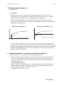
• The spectrometer acquisition time of an X nucleus experiment should be estimated from similar
experiments on the same equipment if possible using eqn (1) or (2) below. 13C and 31P
experiment times on the 500’s and 360 can be estimated from similar experiments on the AC-300
(Athena) using:
S N ∝ cBo3 / 2 t 1 / 2ξ
(1)
where c = concentration, Bo = magnetic field strength, t = experimental time, and ξ = probe filling
factor. To estimate the time under different conditions that would give identical S/N, then:
t new = t old
2

 cold   Boold


⋅ 
 c new   Bo
 new





3
 .


(2)
A reasonable estimate (although direct comparison to experiments on similar compounds is
preferred) on the UWChemMRF equipment can be made starting with the observation that a
0.1 M solution will typically give publication quality spectra in 20 min on the AC -300 (Athena).
• Standard decoupled (NOE-enhanced), quantitative decoupled (no-NOE; Bruker’s INVGATE.AU)
and NOE-enhanced coupled spectra (Bruker’s GATEDEC.AU) can be obtained through use of the
S2PUL sequence.
• Nuclei with negative γ values, such as 15N and 29Si, are best acquired using polarization transfer
sequences; DEPT in general is the preferred sequence over INEPT if more than one JXH value is
involved; quaternary moieties of negative γ nuclei are best obtained through long-range coupling
unless the T1(X) values are known to be reasonably short.
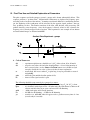
1d
1 3
C Acquisition (s2pul)
UWChemMRF
Experiments - 1H 1d Acquisition
Page 32
B. Critical Parameters
d1
dof
dpwr
dmf
dmm
dm
– relaxation delay; d1 > T1(1H) to obtain optimum NOE
– usually =0 when solvent set correctly; should be within 5ppm of 1H coupled to X
nucleus of interest
– decoupler power (larger number is higher power); typically never > 46
– decoupling strength = [pw90(1H at dpwr)]-1
– decoupler modulation mode; either dmm=’ccp’ dseq=’waltz16’ dres=90 or
dmm=’ccw’ [both are equivalent] is best for typical compounds
– decoupler on/off flag (see Table 6)
C. 1d X{1H} Acquisition
• start by setting the probe parameter appropriately
• to setup parameters (method b is recommended)
a) either read in a data file (rt) or parameter file (rtp) for standard X{1H} acquisition, or
! b) click on MAIN MENU SETUP and select nucleus and solvent
c) alternatively, run s2pul macro (but normally will need to reset spin=’n’, gain=0; check temp
and vttype, and check tpwr (=58 typically) and pw (=5-8µs typically).
• use UWMACROS TUNE PROBE TUNE C13 [or tunec macro] and tune 13C channel; reattach 13C
X cable to X Obs BNC
–
make sure ¼ wave cable is correct for 13C
–
make sure low-pass (brown) filter is in-line
–
make sure correct probe cap is inserted (none in bbold probe)
–
make sure no external attenuator is in-line
• use UWMACROS TUNE PROBE TUNE H1 [or use tuneh macro (will have to reset gain after
tunec if UWmacro is not use] and tune decoupler channel; reattach 1H decoupler cable to
decoupler BNC
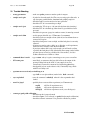
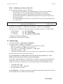
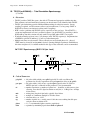
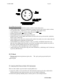
Table 6. Common Decoupler Parameter Settings
Parameter Settings
dm=’yyy’ dpwr=46 su
dm=’nnn’ su
dm=’nny’ su
dm=’yyn’ su
dmm=’p’
dmm=’ccp’
dseq=’waltz16’ dres=90
dseq=’garp1’ dres=1
dmf= [1/pw90]
dpwr= [ typically ~42]
Comments
typical for 13C acquisition; full on decoupler; keep dpwr ≤ 48
turns decoupler off; always finish with this command + su
inverse gated (Bruker’s INVGATE.AU) mode; gives quantitative
(assuming d1>5T1 !) decoupled spectra
gated spectra (Bruker’s GATEDEC.AU); gives coupled spectra but with
NOE buildup (DEPT is necessary for 29Si, 15N and other -γ nuclei)
normal setup for 13C acquisition (8/1/97; dmm=’w’ works fine)
normal setup for DEPT and INEPT most 2d 13C experiments, does hard
pulses followed by pulsed decoupling during acquisition
normal setup for 13C (and all X) acquisitions; 1H waltz-16 decoupling
normal setup for all inverse experiments; X garp-1 decoupling
sets decoupler pulsewidth for composite pulses, where pw90 is the 1H
decoupler 90° pulse width at the dpwr setting used for decoupling
decoupler power in dB; typically want 90° pulsewidth = 100-150µs
UWChemMRF
Varian NMR User’s Guide
Page 33
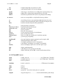
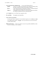
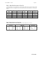
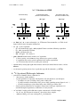
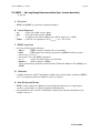
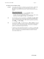
1d
1 3
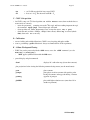
C Variations in VNM R
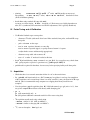
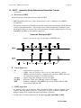
sta ndard setu p
coupled noe acquis.
(B ruker’s G AT E D EC .A U )
qua ntitative dec. acq.
(B ruker’s IN V G ATE .AU )
dm =’yyy’
dm =’yyn’
dm =’nny’
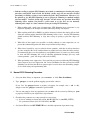
• use dm=’yyy’ su to turn on decoupler (or UWMACRO DECOUPLER ON; see Table 6 and
figure below for more decoupler information)
• use go to start acquisition
– ga will automatically apply a wft (weighted Fourier transform) following acquisition
– use wft to manually transform
– dscale will display the axis
– dsx will apply wft dscale(-3)
• gain = 30 to 40 should usually work for 13C acquisition
–
if always getting ADC OVERLOAD beep, then receiver gain is too high
–
it is important the receiver gain be optimized for X nucleus experiments
–
see 1H section above for how to set the gain accurately
• optimize sw by setting right (right mouse button) and left (left mouse button) cursors, and use
movesw
• set reference by placing cursor close to peak, then type nl rl command, e.g., rl(77p)
D.
13C
(X) pw90 and {1H} Decoupler Calibrations
• general rule of thumb for these calibrations is:
–
short runs use facility numbers
–
if probe problems are suspected, check pw90’s of X and 1H observe (not decouple)
• if numbers are close to facility values, probe is likely OK
• if pw90 is much less than facility value, you are doing something wrong (figure it out! : -)
• if pw90 is much longer (>1µs) than facility value, find TA or facility staff
– always perform calibrations for overnight or longer runs for PT-type experiments; for
standard decoupled experiments, calibrations are rarely needed
• 13C and other X nuclei pw90 calibrations require concentrated or labeled samples
–
for 13C, use 50% benzene in acetone-d6; do not degas these samples
–
addition of GdCl2 or Cr-acac can improve T1’s dramatically
UWChemMRF
Experiments - 1H 1d Acquisition
–
–
–
–
Page 34
set tpwr to desired setting; see Table 2 (on lab wall for most current!!) for calibrations for
probes in UWChemMRF facility
make sure you are on resonance (set cursor on multiplet, then movetof)
set d1=20s or longer depending on sample T1
use 360° pulse for final checks always!!
• once the observe pw90 is obtained, assuming in exp1 then jexp2
– move 1H cable to observe port, and find resonance for benzene doublet (take one scan, move
cursor to middle of doublet and use movetof); write this value of tof down as 1H dof
• assuming 13C still in exp1 and 1H in exp2, do jexp1 mp(3) jexp3
– put 1H on resonance by setting dof = 1H dof from above
– setup decoupler calibration experiment with UW macro pwxdec90
– set pwxlvl = 60 and find pwx where antiphase doublet nulls; this is decoupler hard 90
– set pplvl = pwxlvl and pp = pwx for hetcor and dept experiments
– set pwxlvl appropriately for decoupling (probe dependent; see Table 2 on wall) and find
pwx where antiphase doublet nulls; set dpwr = pwxlvl and dmf = 1/(pwx*1e-6)
E. 1d X{1H} Data Workup and Plotting
• typically will want lb = 2 or 3 for 13C experiments
• see 1d 1H section E for plotting description
UWChemMRF
Varian VNMR User’s Guide
Page 35
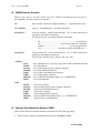
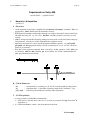
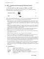
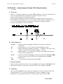
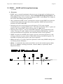
III. DEPT – Distortionless Enhancement by Polarization Transfer
(22-Jun-98)
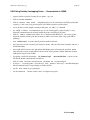
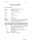
A. Discussion of PT versus NOE experiments, and DEPT versus INEPT
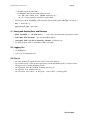
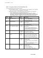
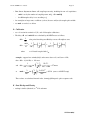
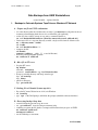
Summarizing Derome (see Chap. 6 for very good discussion, p. 129ff): Polarization transfer
experiments can offer sensitivity enhancements of:
Polarization Transfer
–
γI
γX
NOE
–
1+
(1)
γI
2γ X
(2)
where X is the nucleus being observed (e.g. 13C or 29Si), and I is the enhancing nucleus (usually 1H,
but could also be 19F or 31P). The following generalizations can be followed:
• Polarization transfer is always recommended for nuclei having negative γ values, 29Si, 15N, and
103Rh being three examples. From eq (2) above, the NOE enhancement for these nuclei could
result in 0 signal. PT is also always recommended for low-γ nuclei (e.g., starting 15N and lower in
frequency).
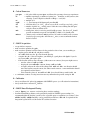
• DEPT is the best method for obtaining 13C spectra, as well as spectra of other spin-1/2 X nuclei,
of typically protonated compounds. DEPT is definitely preferred over INEPT if more than one JXI
value is involved for the nuclei you want to observe.
• DEPT should be used to obtain coupled spectra (turn the decoupler off during the acquisition:
dm=’yyn’); in general, DEPT will give better S/N than coupled NOE experiments.
• DEPT should be used even if no 1-bond coupling to protons are present for low-γ nuclei if longrange couplings can be used.
• INEPT should be used only if one J value is involved and it’s size is known.
• typically, only a DEPT-135 is needed (mult=1.5), but vnmr makes fully edited spectra easy to
obtain; accurate pulse widths are required for good methyl/methine differentiation
• For all these experiments, delays will be dependent on JXI. The better the coupling is known, the
better the experiment will work. Make every attempt to measure the couplings from the isotope
splittings in the 1H spectrum, or obtain good literature values. Lacking both, be prepared to run a
series of experiments using different JXI values to find the optimum parameters.
• For small JXI couplings, a compromise between signal loss from T2 (inverse natural line width)—
especially for low-temp or high MW samples—and PT must be made. In some cases (mainly
when (T1)X is not too large), the non-NOE decoupled (Bruker’s INVGATE) may be the preferred
experiment.
B. Critical Parameters
d1
j
pw, tpwr
pp, pplvl
mult
–
=
–
–
–
relaxation delay; typically = 1-2s
140Hz; change if you want to observe X with JXH>180 Hz or <110 Hz
observe X 90° pulse width pw at power level tpwr
high power 1H 90° pulse width pp at power level pplvl
determine type of DEPT; 0.5 = dept-45, 1.0 = dept-90, 1.5 = dept-135; see
discussion below
UWChemMRF
Varian NMR User’s Guide
Page 36
C. DEPT Acquisition
≤46) and dmf
• for short runs, use facility calibrations for pw, tpwr, pp, pplvl, dpwr (≤
• FILE SETUP SEQUENCES DEPT will setup Dept correctly, including for non-13C acquisitions
–
mult is set by the number of coupled protons
–
the interpulse delay is set according to j
• for overnights or longer runs, recalibrate (at least) observe and (best) decoupler pulse widths
• set mult as needed; dept-135 has mult=1.5; for full editing use array mult=0.5,1.0,1.0,1.5
• use au to acquire for full editing; ga is ok for dept-135
D. Calibration
• see 13C section for nominal 13C (X) and 1H decoupler calibrations
• Often, the best way to calibrate the decoupler is to run a DEPT-90 on a compound having a
known methylene; this carbon should be nulled in a DEPT-90. Change pp (can use an array) to
obtain minimum signal at the methylene, and use on unknown or less concentrated sample.
• The delay d2 and the final decoupler pulsewidth mult*pp are calculated by the DEPT macro
as follows:
D2 =
1
2J
[ use JC-H = 150 if olefinic present, 130 otherwise]
 1 
pp
 (in radians) =
90 o
 n
 −1  1 

 (in deg)
sin 
 n


 −1  1 

1
 (in radians) = o
sin 
 n

 90
 −1  1 

 (in deg) 
sin 
 n


θ pulse ≡ mult*pp = sin −1 
Thus
mult =
2
π
UWChemMRF
Varian VNMR User’s Guide
Page 37
For trimethyl-silyl (JSi-H = 2 Hz),
d2 = 250 msec,
mult =
19.47 o
90 o
= 0.216
These values are calculated internal in the /vnmr/psglib/dept.c pulse sequence code.
E. Data Workup and Plotting
• for full editing, try autodept or padept macro;
• for dept-135, use wft and phase
• s1 (s#) and r1 (r#) are enormously useful for comparing data in different workspaces; use
these in combination with md(1,2) for example to move the save regions in exp1 to exp2
• use clradd spadd to move a spectrum into exp5;
then addi to compare that spectrum with currently displayed spectrum
• use dss with proper vo and ho to give a stack
• pl(‘all’) to plot the stack
UWChemMRF
Experiments - INEPT 1d Acquisition
Page 38
IV. INEPT – Insensitive Nuclei Enhanced by Polarization Transfer
(22-Jun-98)
A. Discussion of INEPT
See the discussion section in the previous section on DEPT.
• INEPT should be used if one J value is involved and it’s size is. Otherwise use of DEPT is
recommended.
• The previous statement is not intended to dissuade students from experimenting with the different
version of polarization transfer. (After all, the fearless facility manager has been known to give
not-such-good advice on occasion. Please do let me know your observation/preferences if you try
both INEPT and DEPT on same/similar compounds.)
Refocused Decoupled INE PT
(in ep trd .c [w ritten b y cg fry ] fro m B ru k er's IN E P T R D .A U )
B. Critical Parameters
d1
j
pw, tpwr
pp, pplvl
mult
– relaxation delay; typically = 1-2s
= 140Hz; change if you want to observe X with JXH>180 Hz or <110 Hz
– INEPT is sensitive to accurate J coupling being entered; use DEPT unless you
are fairly certain you know J reasonably accurately
– observe X 90° pulse width pw at power level tpwr
– high power 1H 90° pulse width pp at power level pplvl
– multipler for d3 delay, where mult= 1 all positive, 2 -CH2- nulled, 3 -CH2inverted from -CH3 and -CH<
C. INEPT Acquisition
• the INEPTRD macro (run by the menu SETUP SEQUENCES INEPT) is not the standard Varian
sequence, but in my opinion is superior; it incorporates all aspects of Bruker’s INEPTRD and
INEPTP sequences for decoupled and coupled acquisition, respectively
≤46) and dmf
• for short runs, use facility calibrations for pw, tpwr, pp, pplvl, dpwr (≤
UWChemMRF
Varian VNMR User’s Guide
Page 39
• FILE SETUP SEQUENCES INEPT will setup Inept correctly, including for non-13C acquisitions
–
mult is set by the number of coupled protons and j ; d3 = mult/4j
–
the d2 interpulse delay is set according to j
• for overnights or longer runs, recalibrate (at least) observe and (best) decoupler pulse widths
• set mult as needed; see below
D. Calibration
• see 13C section for nominal 13C (X) and 1H decoupler calibrations
• The delay d2 and mult*d3 are calculated by the DEPT macro as follows:
1
echo period involving two d2 delays creates 1H antiphase state
4J


mult
1  −1  1 
1  −1  1 
sin
(deg)
=
(rad) =


d3 =
sin 




o
4J
2πJ 
 n
 n
 360 J 

d2 =
where
n = # I nuclei coupled with JXH
example: suppose have trimethylsilyl, and want to detect 29Si, and JSi-H = 2 Hz,
then d2 = 1/(4×2 Hz) = 125 msec
1 
19.47 o
sin 
 =
= 27 m sec
and d3 =
o
360 o × 2Hz
 9  360 × 2Hz
1
or
mult =
−1 
o
−1  1  2 × 19.47


sin
=
= 0.216 (same as in DEPT setup)


180 o
180 o
 9
2
These values are calculated internal in the /vnmr/psglib/ineptrd.c pulse sequence code.
E. Data Workup and Plotting
• workup is similar (identical) to 13C 1d and DEPT
UWChemMRF
Experiments - NOEDIFF 1d Acquisition
Page 40
V. 1d NOE-Difference Spectroscopy
(24-Dec-97)
A. Discussion
• See the Bruker User’s Guide introduction for discussion on this non-trivial, but powerful
experiment.
• Sanders & Hunter also contain excellent discussions on NOE experiments (highly recommended)
• Look for instructions on use of GOESY, which should be significant improvement over NOEdiff.
B. Critical Parameters
d1
dpwr
dm=’yyn’
dof
– relaxation delay; needs to be ≥ 3 T1 (see later section for measuring T1)
– must not be set above 14; typically 1-4 works well for saturating multiplets
– typical, but dm=’nyn’ and d2 can be used to vary saturation within fixed
d1+d2 delays
– set by command sd (preceded by placing cursor on desired multiplet)
C. NOE-Diff Acquisition
• read in a normal 1H setup: MAINMENU SETUP NUCLEUS/SOLVENT
• SETUP SEQUENCE NOEDIFF will setup the following parameters:
dn=’H1’ homo=’y’ dmm=’c’ dpwr=1 dm=’yyn’
• place the cursor in the middle of the multiplet to be saturated and enter sd
• obtain enough data to determine
i) if multiplet is being sufficiently saturated
ii) if any other close-by multiplets are being effected by the saturation pulse; if any are, dpwr
must be decreased until the close-by multiplets are all completely uneffected; this condition
is essential–interpretation of the data becomes much more difficult if the chosen multiplet
cannot be saturated independent of the other protons (if this happens, consider performing a
NOESY or ROESY experiment instead of the NOE-diff)
iii) currently, I do not know how to plot or save difference spectra if dof is arrayed (although
this would seem to be the best way to acquire the data)
iii) see cgfry about implementation of GOESY, which should be a superior experiment to
NOEdiff; GOESY info should be available very soon
D. Calibration
• set dpwr low, and raise by 3 dB to no more than dpwr=14; use the lowest power that saturates the
selected multiplet
E. Data Workup and Plotting
• bring in reference spectrum (with decoupler placed on baseline); make sure expansion and vertical
scale are what you want
• make sure exp5 is saved and not in current use, then
• use clradd spadd to clear exp5 and transfer the current spectrum to it
• bring in next spectrum (in another exp if desired, but must have same expansion and vs; more
precisely, sp wp vs must all be identical between spectra)
• use addi to compare and subtract spectra; see vnmr manuals for more info
UWChemMRF
Varian VNMR User’s Guide
Page 41
VI. Homonuclear 1d Decoupling
(1-Jul-98)
A. Discussion
• HOMODEC has for the most part been replaced by COSY and cosy-variants, but still has utility for
multiplets that are well resolved. HOMODEC can provide actual J couplings, whereas fast-COSY
usually does not.
B. Critical Parameters
d1
dpwr
dm=’yyy’
dof
–
–
–
–
relaxation delay; needs to be ≥ 3 T1 (see later section for measuring T1)
must not be set above 24; typically 1-14 works well for saturating multiplets
correct for homodecoupling
set by command sd (preceded by placing cursor on desired multiplet); can array
this variable to obtain all homodec’s in same experiment
C. Acquisition
• setup using SETUP SEQUENCES HOMODEC (or just type in homodec to run the macro)
dn=’H1’ homo=’y’ dmm=’c’ dpwr=1 dm=’yyy’
• array the dof values to acquire all in one experiment
• once decoupler is on, simply use go or ga
D. Calibration
• adjust dpwr (≤14) to reduce multiplet without spilling into close-by multiplets
E. Data Workup and Plotting
• workup as a standard 1H
• dssa should be useful for plotting; see vnmr documentation
UWChemMRF
Experiments - COSY 2d Acquisition
Page 42
VII. COSY – 2d Homonuclear Correlation
(21-Jul-01)
A. Discussion
• Absolute value mode COSY often provides sufficient homonuclear correlation data in a very
efficient, robust experiment.
• JHH ≥ 4 Hz can typically be observed, but this is dependent on sw and ni
digital resolution in F 2 =
sw
np
digital resolution in F1 =
sw1
2ni
assuming zero-filling only in F1 (not common in F2). For very large ni, very small couplings can
be observed—often well below the linewidth of a high-resolution 1D experiment.
• A common rule-of-thumb is that JHH ≥ dres1/3 will be observed in a COSY spectrum; this
estimate is definitely a guideline only. dres1 ≡ digital resolution in F1 defined above.
• The most efficient method of observing small JHH is with long-range COSY, which involves this
sequence and tau > 0 (typically tau = 50-200 ms).
• cosy loses sensitivity from the strong resolution enhancing sinebell (and sinebell-squared)
apodization functions used to overcome the absolute value processing. Even so, minimum phase
cycling (nt=4) usually gives sufficient sensitivity. GCOSY is even faster (nt=1, nt=2 is better).
• DQF-COSY (next section) removes all singlets, and gives much cleaner diagonals. Use this
sequence after a COSY if crosspeaks close to the diagonal or on a strong singlet region are
needed.
• gcosy is preferred if a PFG (e.g., hcx or bbswg) probe is installed. nt=1 can be used with this
sequence, reducing total acquisition time by 4.
B. Critical Parameters
p1
ni
nt
sw
sw1
= 90° for maximum sensitivity; 45° (typical) to reduce intermultiplet crosspeaks
= usually set satisfactorily by cosy macro; sw1/2ni gives usable resolution; must
have ≤ 12 Hz, but want ~ 6 Hz if time allows for best results
= 4 is minimum phase cycle
= set using movesw macro (preceeded by boxing selected area of spectrum)
= must equal sw for foldt macro (commonly used; recommended for fast-COSY)
UWChemMRF
Varian VNMR User’s Guide
tau
d1
Page 43
= set 50-150 ms typical for long -range COSY
= best set ≥ 2×T1, but often run with d1 ~ T1
C. COSY 2d Acquisition
• for COSY, setup as in 1H 1d and optimize sw with the movesw macro, then retake the data to
ensure sw is set correctly
– move the parameters: assuming you ran the 1H in exp1 and have nothing important in exp2,
the command mp(2) jexp2 entered from exp1 will work
– from exp2 then use SETUP SEQUENCES COSY or enter the macro cosy or gcosy
– check that ni (sw1/2ni ≤ 12Hz/pt, ~6Hz/pt if time allows) d1 and np are correct (check
time), then enter au to run cosy
D. Calibrations
• can use facility pulse width calibrations; COSY is very forgiving with pulse widths
• even so, performing a pw90 calibration is always recommended for all 2d experiments
E. 2d Data Workup and Plotting
• COSY data can be processed with the do2d macro, or use the wft2d command (see also
man(‘cosy’) or man(‘gcosy’)
do2d applies symmetrization with the foldt macro
–
• general display and plot commands
dconi
; displays 2d’s with color map (faster than contours)
plot projections before issuing the following command using menus (use the PLOT button)
pcon
pconpos
pconneg
plot2dhr
; plots contours
; plots phase sensitive contours with positive peaks
having 10 contours and neg peaks having 1 contour
; opposite of pconpos
; plots with high-resolution traces (must have 1d in
another experiment)
UWChemMRF
Experiments - DQ-COSY 2d Acquisition
Page 44
VIII. DQ-COSY – Double-Quantum Filtered COSY (Phase-Sensitive)
(17-Jul-00)
A. Discussion
• DQCOSY is currently accepted by most in the NMR community as the most powerful form of
COSY; it is recommended for any experiment beyond the FAST-COSY or GCOSY
• removes singlets (important for strong solvent peaks)
• diagonal in pure adsorption mode with crosspeaks (cleans diagonal for close-in crosspeaks)
• direct coupling (for crosspeak at ν1,ν2 is J1,2) is anti-phase, whereas indirect coupling (at ν1,ν2 is
J1,3 or J1,4, for example) is in-phase, allowing for J assignments in complex molecules
• alternative experiment is E. COSY (see section X)
B. Critical Parameters
pw, tpwr
d1
ni
np
fn fn1
nt
sspul
= 90° pulse width at power tpwr; recalibrate this parameter for all dqcosy
experiments
= relaxation delay; set 2-3*T1 (artifacts will result if d1 is too small)
= number experiments, or number of points in t1 ; should be set ok by macro, time
allowing; want F1 digital resolution ≤ 6 Hz/pt = sw1/(2ni)
= number of points in t2, usually want ≥ 2048 since costs nothing but disk space
and gives better resolution in F2
≠fn
= usual to not zerofill in F2 (fn=np), and give one zerofill in F1 (fn1=2ni); fn1≠
is ok for DQCOSY, but to baseline correct in both dimensions set fn1=fn
= multiple of 8
= ‘y’ gives homospoil-90-homospoil preceding d1
C. dqcosy Acquisition
• DQCOSY is setup essentially the same as COSY (use dqcosy macro) except want fn=np≥2048 and
typically ni ≥ 350 (ni is set up by macro; check that F1 dig resol ≤ 6 Hz/pt = sw1/(2ni))
D. Calibration
• always recalibrate pw90 (90° pulse) for dqcosy (experiment is sensitive to quality of this easilycalibrated parameter—see 1H section for instructions); macro uses pw90 to set pw
• with high-res 1d, or perhaps better ni=2 run, carefully baseline correct, then run calfa
UWChemMRF
Varian VNMR User’s Guide
Page 45
E. Phase-Sensitive 2d Data Workup and Plotting
• often should not need to phase DQCOSY data at all
• phase sensitive data should be processed something like the following:
– set pmode=’full’
; allows phasing along F2 in 2d spectrum
–
wft(1)
; transform just first spectrum
–
wtia
; interactive phasing; middle button scales, left sets lb
–
wft1da
; perform first transform (on t2 dimension)
–
if integrals have been setup (best on high-res 1d done prior to setting up dqcosy), then
bc(‘f2’) can sometimes work wonders here
–
click on TRACE and select strong intensity trace
; trace=’f1’ changes columns→rows, trace=’f2’ goes back
–
wtia
; interactive phasing on t1 trace, left button sets lb/gf
–
wft2da
; performs second (or both) transform(s)
–
pick off two traces that have crosspeaks
–
ds(r1) do 0-order phase only
–
ds(r2) do 1st-order phase only (click left mouse button on downfield position sets toggle pt)
–
iterate between ds(r1) and ds(r2) to get good phase
–
dconi
; downfield trace save number as r1
; upfield trace save number as r2
; should now have good phasing
→ trace=’f2’ dconi allows phasing along F2 (similar to above) if needed
–
if integrals have been setup (as above), and only if fn1=fn, then bc(‘f1’) can sometimes
work wonders here
–
to plot, plot2dhr is a new macro that works quite well; if you want 1d projections, load the
high-resolution 1d into a separate experiment before issuing the macro command. Otherwise,
I like parameters: wc=130 wc2=wc sc=0 ; this leaves room for a vertical projection or to
print parameters on the page (use disp2d to set these)
–
maximum printable parameters on 8.5×11 paper are wc=230 wc2=150
–
rl(..p) gives F2 referencing, rl1(..p) gives F1 reference
–
use plot2dhr (preferred) or pconpos or pconneg to plot phase sensitive spectra
UWChemMRF
Experiments - TOCSY 2d Acquisition
Page 46
IX. TOCSY (or HOHAHA) – Total Correlation Spectroscopy
(17-Jul-00)
A. Discussion
• TOCSY provides COSY-like spectra, but with all 1H connected appropriate with the mix time.
Thus, mixtures and small molecular fragments can often be more easily identified with TOCSY.
• TOCSY spin-lock mixing provides Hartman-Hahn matching for coherence transfer. Strong
coupling is required, and off-resonance effects can be troublesome. Use long-range COSY or
DQCOSY to observe correlations involving small J-couplings.
• ROE’s can be a problem with TOCSY spectra, especially as mix gets large. Clean-TOCSY, a
variant not implemented in Varian’s standard sequence, can offset ROE’s by providing a similar
NOE build-up, but this variation will only work for large MW where NOE’s are negative.
• Watch the manual page [man(‘tocsy’)] for changes in the TOCSY sequence(s). Implementation
of DISPSI-2 spin-lock is underway, as well as gradient homospoils.
• Multiple mix times are often useful. These cannot be run arrayed with phase=1,2; phase=3
(TPPI) must be selected if arraying mix is desired. Queuing multiple experiments with different
mix times and phase=1,2 is another method for this type of data collection, and is recommended.
2d TO CSY Spectroscopy (M LE V-16 Spin Lock)
n
B. Critical Parameters
p1, p1lvl
pw, tpwr
ni
mix
nt
d1
np
phase
trim
= 90° pulse width at high power p1lvl (typically 52 to 60); recalibrate this
parameter for all tocsy experiments (uses pw, tpwr from 1d to set p1, p1lvl)
= 90° pulse width (~20 to 40 µs) at power tpwr (typically 46 to 52) used for
MLEV spin lock; calibration of this parameter is also recommended
= number experiments, or number of points in t1 ; should be set ok by macro, time
allowing; must have F1 digital resolution ≡ sw1/(2ni) ≤ 12 Hz/pt but ~ 6 Hz/pt
if time allows
= mixing time (length of spin lock), typically 30 to 100 ms
= multiple of 2 minimum, multiple of 4 if time allows
= relaxation delay; set 1-2*T1
= number of points in t2, usually want ≥ 1024 since costs nothing but disk space
and gives better resolution in F2
= 1,2 is recommended (phase-sensitive acquisition)
= optimize by minimizing signal when d2=0 and phase=2
UWChemMRF
Varian VNMR User’s Guide
Page 47
C. TOCSY Acquisition
• prior to final setup, run ni=2 and carefully phase t2 spectrum
– then enter calfa and reacquire; observe baseline flattening
– perform integrations on 1st increment if baseline correction is desired
• check that nt=multiple of 4 (2 can be used if time is critical)
• check that F1 dig resol ≡ sw1/2ni ≤ 12 Hz/pt, desire ~6 Hz/pt if time allows
• check that p1,p1lvl are set appropriately (should equal pw, tpwr from 1d 1H experiment—I will
likely change this confusing definition during the DIPSI implementation), and pw,tpwr are set to
give pw90 ≥ 20µs
• set window = 2pw (clean-tocsy only), and optimize trim by mp(current exp#+1), phase=2
and d2=0, then choose trim giving minimized signal
D. Calibration
• recalibrate 90° pulses for p1,p1lvl and pw,tpwr (see 1H section for instructions) for longer
experiments; short/quick experiments can be run with probe file calibrations and macro setup
E. Data Workup and Plotting
• same as dqcosy (see DQCOSY section for phase-sensitive workup)
UWChemMRF
Varian VNMR User’s Guide
Page 48
X. Other COSY Variants
(21-Jul-98)
A. Discussion
• E-COSY can provide a good alternative to dqcosy for determining coupling constants
E-COSY has the advantage that fewer crosspeaks are present, but all coupling information is
–
still present
E-COSY has the disadvantage that the minimum phase cycle is very large (32), so the
–
experiment can take much longer that necessary from S/N considerations
–
see van de Ven for an excellent discussion on E-COSY and other variants
–
gradient E-COSY may provide a usable form of E-COSY; look for more details
• see COSY for long-range and relayed experiments
B. Critical Parameters
• section not ready yet
C. Acquisition
• section not ready yet
D. Calibration
• section not ready yet
E. Data Workup and Plotting
• section not ready yet
UWChemMRF
Experiments - NOESY 2d Acquisition
Page 49
XI. NOESY – 2d NOE and Exchange Spectroscopy
(17-Jul-00)
A. Discussion
• NOESY can be a powerful experiment for the correct types of compounds, and with proper care
during acquisition and analysis of the data. Care is recommended during interpretations! See
Sanders&Hunter Chap. 6 for an excellent introduction to NOE’s; see the Bruker User’s Guide for
more details about NOE experiment particulars.
• Often, combinations of MW, solvent, and temperature conspire to make NOESY crosspeaks nonrealizable during nominal mix time in this transient experiment. ROESY will often be better
alternatives for small (≤2000) MW.
• Performing at the least an inversion-recovery null-estimate of 1H T1 values is highly
recommended prior to acquiring NOESY spectra. This method of obtaining 1H T1’s is quick, and
simple to setup. Perform full T1 analysis for best results (see dot1 macro).
• Degassing leads to longer T1 values for smaller MW compounds, and is recommended for 1D
variants. The longer T1 values, which can lead to greatly enhanced NOE build-ups, sometimes
cannot be maintained for 2D experiments, due to limitations in time for the experiment.
• NOESY crosspeaks for small MW will be positive (opposite to the inverted diagonals) as will
exchange crosspeaks (use temp variation to differentiate exchange from NOE crosspeaks). For
larger MW, crosspeaks will be negative (same sign as diagonals).
• Multiple mix times (≤ T1) will be required for quantitative work in using NOESY build-up curves
for obtaining distance information.
• ulnoesy is recommended (but currently unavailable) over the vnmr standard sequence noesy.
For now, use tnnoesy if needing presaturation, otherwise noesy (or equivalently SETUP
SEQUENCES NOESY).
UWChemMRF
Varian NMR User’s Guide
Page 50
B. Critical Parameters
pw, tpwr
ni
nt
sspul
d1
np
mix
mixvar
= 90° pulse width at power tpwr; recalibrate this parameter for noesy experiments
= number experiments, or number of points in t1 ; should be set ok by macro, time
allowing; want F1 digital resolution ≤ 6 Hz/pt = sw1/(2ni)
= multiple of 8
= ‘y’ gives homospoil-90-homospoil preceding d1
= relaxation delay; set 2-4*T1 (do not set too small, or will get very bad t1 noise)
= number of points in t2, usually want ≥ 2048 since costs nothing but disk space
and gives better resolution in F2
= mixing time; often is varied to provide build-up curves. Set close to T1 should
provide maximized crosspeaks; for high MW (>2000) ~0.3s should work.
= (ulnoesy only) variation in mix in percent; 10 works reasonably well to remove
cosy/tocsy type crosspeaks; will increase t1 noise, so not recommended unless
know is needed
C. NOESY Acquisition
• set-up similar to DQCOSY
• make certain to optimize the gain
• make certain to optimize baseline flatness for the particular value of sw you are working at:
–
acquire spectra with ni = 2, and phase carefully
–
run calfa which uses the lp value from the phasing
–
reacquire the ni = 2 data and rephase; you should get a good phase with lp=0; if you do
not, rerun calfa and require again
–
if the baseline still has some curvature (either convex or concave), then you might want to:
– note the values of rof2 and alfa
– keeping the sum rof2+alfa constant, change rof2 and alfa
– reacquire and note the effect of the change with rof2 and alfa; one direction should
move the baseline towards convex, the other towards concave; some combination should
give optimal baseline flatness
– write down the values of sw rof2 and alfa; these should always work for this sw
• as a minimum, estimate T1 using inversion-recovery null method to provide setting for d1
D. Calibration
• always recalibrate 90° pulses for pw,tpwr with NOESY spectra (see 1H section for instructions)
• always work from a measured T1 estimate
E. NOESY Data Workup and Plotting
• same as dqcosy (see DQCOSY section for phase-sensitive workup)
• baseline flatten/fitting routines can be particularly useful for NOESY spectra workup; it is
recommended that the baseline is made as flat as possible prior to acquisition (see section C), but
wft1da bc(‘f2’) wft2da bc(‘f1’) can be particularly useful here; fn1 = fn is required for the
integration regions in F2 to work for the F1 baseline correction
UWChemMRF
Experiments - ROESY 2d Acquisition
Page 51
XII. ROESY – 2d NOE Spec.; Mixing via a Spinlock in the Rotating Frame
(17-Jul-00)
A. Discussion
• ROESY spectra will produce a maximum +0.5 enhancement for 1H independent of MW. The
experiment is still transient (as in NOESY), however, so enhancements are always smaller than
0.5. As always with NOE/ROE experiments, absence of a crosspeak does not confirm lack of
proximity (see Sanders & Hunter for a good introduction on this subject).
• An ROE is produced by inverted magnetization created via chemical shift during t1 (d2) and
locked to the y’ axis by the pulsatile spin-lock during the mix time. pw should be set at 30°, and
ratio set to ~6 for tpwr ~ 52 on bbswg probe.
B. Critical Parameters
p1, p1lvl
pw, tpwr
ratio
= 90° pulse width at power p1lvl; recalibrate this parameter for roesy experiments
= 30° pulse width at power tpwr; recalibrate this parameter for roesy experiments
= number of pw with no rf between actual pw pulses; usually set ~6 (should be ≥5)
The spinlock field strength used in this type of experiment (Kessler spinlock) is:
B1sl =
ni
nt
sspul
d1
np
mix
1
pw360 (ratio + 1)
Type slroesy to get the spinlock power for a particular ratio and pw.
= number experiments, or number of points in t1 ; should be set ok by macro, time
allowing; want F1 digital resolution sw1/(2ni) = 6 Hz/pt
= multiple of 2, multiple of 8 preferred
= ‘y’ gives homopoil90-homospoil preceding d1
= relaxation delay; set 2-3*T1 (do not set too short, or will get very bad t1 noise)
= number of points in t2, usually want ≥ 2048 since costs nothing but disk space
and gives better resolution in F2
= mixing time; often is varied to provide build-up curves. Set close to T1 should
provide maximized crosspeaks; for high MW (>2000) NOESY is preferred.
C. ROESY Acquisition
• see NOESY section; adjust baseline similarly, and make certain to use actual ROESY sequence
(do this by setting ni=2) when performing the calfa correction
UWChemMRF
Varian NMR User’s Guide
Page 52
D. Calibration
• calibrate pw, tpwr, p1, p1lvl for all ROESY experiments
• watch out for coupling partners that are centered in the spectrum; these will give TOCSY
crosspeaks in a ROESY; in this case, change tof to get the coupling pair off-center
E. Data Workup and Plotting
• same as dqcosy; see DQCOSY section for phase-sensitive work-ups
UWChemMRF
Varian VNMR User’s Guide
Page 53
XIII. HETCOR – 2d Heterocorrelation Spec. (“normal” X nucleus detection)
(27-Dec-97)
A. Discussion
• typically want to run HMQC (see next section) or HSQC, as dramatic improvement in S/N is
obtained in the inverse experiments
• HETCOR is still run when high digital resolution is needed in the X dimension; a common example
would be 13C-1H correlation spectroscopy where resolved closely grouped aromatic 13C are
needed to improve assignments of the aromatic protons
B. Critical Parameters
• section not ready yet
C. HETCOR Acquisition
• section not ready yet
D. Calibration
• section not ready yet
E. Data Workup and Plotting
• section not ready yet
UWChemMRF
Experiments - HMQC 2d Acquisition
Page 54
XIV.HMQC and HSQC – 2d Heteronuclear Spectroscopy (“inverse” experiment
with 1H detection)
(20-Jul-01)
A. Discussion
• Two sequences for measuring 1H-X chemical shift correlations, gHSQC and gHMQC are very
similar, and both will work fine for most organic compounds.
• HSQC will give sharper lines, especially for –CH2– since 1H–1H homonuclear coupling in the F1
axis is not suppressed in HMQC. HSQC is more sensitive to pulse width calibrations (has more
π-pulses), but HMQC can suffer T2 sensitivity losses in viscous and high-MW compounds.
• Gradient sequences are typically superior in S/N, especially for long-range HMBC.
B. Critical Parameters
• pw – 1H 90° pulse width at power tpwr
• pwx – X 90° pulse width at power pwxlvl
• j1xh – J-coupling for correlations of interest, set to 140Hz for 1-bond HSQC and HMQC
experiments (see HMBC for long-range experiments)
• ni
– fixes the digital resolution in F1, dres1 = sw1/(2ni); because of the large J-coupling in
1-bond experiments, dres1 need only provide sufficient resolution for 13C chem shift,
and is therefore set larger than typical in a COSY experiment. For COSY, dres1 =
4 Hz/pt, where in HSQC/HMQC dres1 ≥ 30 Hz/pt is usually sufficient.
• d1 – best set ≥ 2×T1, but not uncommon to run at ~1.5×T1
• sw1, dof – sets the 13C F1 spectral axis; set the next section as to how to set
C. HMQC Acquisition
• for long HMQC runs, or lossy samples, calibrate the 13C decoupler using a 13C-enriched sample
and PWXDEC90 sequence (see section D below)
• tune the probe at 13C then 1H for your sample
• acquire a standard 1H spectrum and optimize sw using movesw
• calibrate pw90 by arraying pw; make certain d1 is not too small (~1.5×T1)
• optimize the gain for pw=pw90 and acquire a 1H high resolution spectrum at the optimized sw
• mp(3) ; assuming started in exp1
• jexp2 and obtain just enough 13C (X cable to observe port) to see the solvent peaks (nt=1 usually)
– if in D2O, you can rely on setref for approximate referencing, or use decref if the 1H
spectrum has a good reference
• optimize sw of 13C by estimating where protonated carbons will show for your compound and
using movesw ga
• jexp3 and type gHMQC or gHSQC; enter 2 when asked where 13C parameters are
• check that pwx, pwxlvl, dmf and dpwr are set correctly
• check j and d1
• check ni and nt
• if running hmqc instead of gradient sequences, optimize null (set ni = 1 and array null ~ T1 )
or use null=0.7*T1 if you know T1 (especially important for solvent if working in nondeuterated solvent)
• au
UWChemMRF
Varian VNMR User’s Guide
Page 55
D. Calibration
• general rule of thumb for these calibrations is:
–
short runs, check proton pw90, for pwx,pwxlvl use facility numbers
–
if probe problems are suspected, check pw90’s of X and 1H observe (not decouple)
• if numbers are close to facility values, probe is likely OK
• if pw90 is much less than facility value, you are doing something wrong (figure it out! : -)
• if pw90 is much longer (>1µs) than facility value, find TA or facility staff
– perform calibrations for overnight or longer runs for HMQC/HSQC experiments
• tune probe at 13C then 1H for 13C enriched sample (13CH3I—Indirect 1—or NaOAc-13C)
• calibrate pw90 for 1H as normal
– set tpwr to desired setting; see /vnmr/probes/probe/probe for most current
–
make sure you are on resonance: set cursor on 12CH3*I singlet (surrounded by 13CH3*I, so
looks somewhat like a triplet) , then movetof
–
set d1=1 at=1 for Indirect 1 samplpe
–
use 360° pulse for final checks always!!
• once observe pw90 is obtained, assuming in exp1 then jexp2
• obtain 13C in exp2 (move X cable to observe port) and place 13C*H3I quartet on resonance (place
cursor in middle or quartet and movetof)
• jexp3 mf(1,3) wft; put 13C on resonance by setting dof = 13C tof from above
– setup decoupler calibration experiment with UW macro pwxdec90 ; check tof and dof
– check pwxlvl = 58 and find pwx where antiphase doublet nulls; this is decoupler hard 90
– set pwxlvl (~46) appropriately for decoupling (probe dependent; see Table on wall or
/vnmr/probes/probe/probe) and find pwx where antiphase doublet nulls; set dpwr = pwxlvl
and dmf = 1/(pwx*1e-6)
E. Data Workup and Plotting
• work-up essentially identically to dqcosy (see end of DQCOSY section for phase-sensitive work-up)
UWChemMRF
Varian VNMR User’s Guide
Page 56
XV. HMBC – 2d Long-Range Heterocorrelation Spec. (inverse detection)
(4-Aug-98)
A. Discussion
• HMBC and gHMBC are powerful assignment techniques
B. Critical Parameters
•
•
•
•
pw
pwx
j
taumb
–
–
–
–
1H
90° pulse width at power tpwr
X 90° pulse width at power pwxlvl
J-coupling for one-bond couplings (these will be suppressed; ~140 Hz)
0.5-0.6 for 13C experiments (=1/2Jlong-range); use ~ 0.1 for 15N
C. HMBC Acquisition
• the macro should setup the following:
– dm=’n’
; HMBC cannot be acquired with 13C decoupling
– null=0
; BIRD suppression cannot be performed (so gHMBC should be superior)
– increase at = 0.3 to 0.4 s
– increase nt ≈ 8×nt from HMQC experiment
– ss = -4
; steady-state pulses before every increment
– mbond=’y’ ; defines sequence as HMQC
– always perform linear prediction (use button under UWMACROS MORE) in F1 on HMQC and
HMBC
D. Calibration
• excellent calibrations of both 1H pw90/tpwr (should always be done before acquiring an HMBC)
and 13C pwx/pwxlvl (calibration should be recent) are required
E. Data Workup and Plotting
• HMBC is often worked in av ph1 mode even though both dimensions are acquired phasesensitive; gaussian filters are typically applied in both dimensions
• linear prediction in F1 to 4×ni is recommended; resolution and sensitivity should increase by
roughly a factor of 2
UWChemMRF
Experiments - Other Hetero. Correlation Exps.
Page 57
XVI.Other Heteronuclear Correlation Experiments
A. Discussion
• section not ready yet
B. Critical Parameters
• section not ready yet
C. DEPT Acquisition
• section not ready yet
D. Calibration
• section not ready yet
E. Data Workup and Plotting
• section not ready yet
UWChemMRF
Spin-Lattice Relaxation, T1
Page 58
XVII.Fitting Partially Overlapping Peaks – Deconvolution in VNMR
•
prepare baseline region by clearing all reset points: type cz
•
click on PARTIAL INTEGRALS
•
click on DISPLAY NEXT RESET and pick integrals over all sections that are NOT good baseline
regions (i.e., this is not to get good integrals, but to define regions of good baseline)
•
resave the data to allow simple restarting at this point; use svf(‘...’) command
•
use bc(5) or similar; I recommend you not use bc which applies a spline fit (this is a very
dangerous command that can seriously modify the shapes and integrals of peaks)
•
click on DISPLAY INTERACTIVE NEXT TH to change the threshold level; you want to go just
below the smallest obvious peak, but not down to where a lot of noise from a large peak will be
picked up
•
enter mark(‘reset’) to ensure that all previous marks are deleted
•
move the cursor to each “normal” peak and press MARK (this enter the center frequency and uses a
default linewidth)
•
move right and left cursor to the approximate half-height points of broad peaks and click MARK
(this enters the average of right and left cursors for the center position, and the difference between
right and left cursors as the width)
•
by opening a shell tool and entering cd ~/vnmrsys/exp1
file that the MARK command built and will use
•
click on MAIN ANALYZE DECONVOLUTE USE MARK FIT
•
if you get a “too many points” error message, enter FN=FN/2 WFT BC(5) and click through to
the FIT command again; keep reducing FN until it will fit
•
use the PLOT button to get a quick plot
•
use the commands
CLRADD SPADD ADDI
more mark1d.out
you can see the
to perform the fit
to compare two spectra
UWChemMRF
Spin-Lattice Relaxation, T1
Page 59
XIX.1H Spin-Lattice Relaxation, T1
(updated 00.07.19)
I. Discussion
• Spin-lattice relaxation, T1, is nominally an exponential process, and is important as the
determining factor in all experiments’ repetition delay, d1. Suggestions for how “abusable”
(borrowed from Varian) d1 is for various experiments is provided below.
• T1 becomes critically important for any quantitative, exchange, or cross-relaxation type of
experiment such as NOE. The relaxation from zero magnetization and from an inversion pulse are
both shown in the figures below.
Recovery from M (0) = 0
Recovery from M (0) = –M o
Mo
Mo
0
T 1 = τ1 /2 /ln 2
M ( τ) = M o [1 -ex p (- τ/ T 1 )]
τ1/2
0
τ
-M o
τn
τ
T 1 = τn /ln 2
M ( τ) = M o [1 -2 ex p (- τ/ T 1 )]
• Usually a quick determination of the T1 is sufficient; this allows proper setting the repetition
delay, d1. For most liquids, use the rapid, inversion-recovery method in Section II below. This
method involves finding the time at which the magnetization goes through a null, τn, as shown in
the figure on the right below. More accurate determinations of T1 must utilize multi-point
fitting, as described in section III.
Rapid Determination of T1 by Inversion-Recovery Null Method
II.
(good for any sample—e.g. any liquid—but is semi-quantitative at best)
•
•
•
•
•
Obtain a reasonable quality 1H spectrum. Locate protons of interest for visual observation.
180° and 90° pulse lengths must be reasonably accurate. If your sample is highly polar (e.g.,
ionic water solution), you must calibrate beforehand. Otherwise, if tuned correctly, prior
calibrations can be used.
set p1=2*pw90 pw=pw90
d2=0.01 should give large negative peaks. Lengthen d2 until proton peaks of interest are
nulled (slightly shorter d2 should give negative peaks; slightly longer should give positive
peaks). For the nulled d2n, T1 ≅ d2n/ln2 = d2n*1.44.
Find d2n for other protons of interest.
UWChemMRF
Varian NMR User’s Guide
Page 60
III. Quantitative measurement of T1 by Inversion Recovery Method
A. Comments
•
•
•
A reasonable estimate of T1 must be known to correctly setup: use the Inversion-Recovery Null
Method (Section II).
180° and 90° pulse lengths must be accurate.
For precise measurements, use d1 = 10 T1; d1 = 5 T1 will provide reasonable values if
experimental times get long. The number of d2 values, nd2, can also be decreased to lessen
experimental times ≅ nt*nd2*(2*d1)
B. Acquisition Set-up
1. use the macro dot1; some randomization of the selected d2 values might be preferable
2. ensure d1> 5 * T1
Table I. A reasonable grouping of VD delays for Inversion-Recovery T1 sequence,
where T1r is the T1 estimate (from inv-rec estimate or a repetition-rate
experiment).
0.01T1r
10T1r
2T1r
0.3T1r
10T1r
0.7T1r
1.0T1r
0.5T1r
10T1r
5T1r
0.1T1r
0.01T1r
1.4T1r
10T1r
C. T1 Analysis (see Varian Subject manual, Adv. 1d section)
1. Expand about the peak(s) of interest. Adjust the threshold with the Th.
2. Enter dpf or dll then fp to locate the peak(s) and then find them through the relaxation set. fp
writes a text file fp.out in the current experiment, e.g., ~/vnmrsys/exp1/ft.out.
3. If the dataset is a T1 set, enter t1; for T2 enter t2, or for a solid-state T1ρ enter
analyze('expfit','p3','t2','list')
4. t1 and t2 will display the information on the bottom of the screen. To print, repeat using, e.g.,
printon t1 printoff
or
print the file ~/vnmrsys/exp#/analyze.list text file (same information) from the File Manager, or
in vnmr with ptext('analyze.list')
5. Show a plot of the data using expl, and plot with pexpl page. Note that you can look at specific
peaks using expl(3) and pexpl(3) page as an example for the 3rd peak. To make a smaller
plot use the sequence expl center pexpl page. To delete a point from the analysis, use
dels(<data#>) fp t1 or similar command.
UWChemMRF
Varian VNMR User’s Guide
Page 61
D. T1 “Abusability” vs Experiment Repetition (d1)
[from Varian course notes]
Likelihood of artifacts increases as go down column.
normal 1d
COSY (magnitude mode)
T1 at 30° pulse
< 1 × T1
INADEQUATE
HMQC & HMBC
HOM2DJ
HET2DJ
HETCOR
COSYPS
TOCSY
NOESY & ROESY (qualitative)
NOESY & ROESY (quantitative)
> 1-1.5 × T1 (13C)
> 1.5? × T1
DQ-COSY & MQ-COSY
Quantitative T1
> 3 × T1 (+ “homospoil”)
≥ 5 × T1
~2-3 × T1
> 3-5 × T1
UWChemMRF
CP/MAS NMR
Page 62
XIX. Cross-Polarization/Magic-Angle-Spinning NMR
(5-Mar-96)
I. Computer Set-Up
• Login, enter acqi in the dialog box; use right mouse on background to bring up acquisition status
box
• Typically, all zero shims (see with dgs) will work fine for solids
• Read in the file cpmas-setup.fid in /usr/fry directory for first run
• set gain=0 temp='n' vttype=0 su (better, use tempoff macro)
II. Sample Set-Up
• Pack sample into rotor with special care for keeping
radial symmetry during packing.
• The caps must fit all the way on; even a bit too much
sample keeping the cap slightly off will prevent smooth
spinning.
• Note the flutes on both caps face the same direction,
with drive air coming from the right (flutes clockwise
looking down onto rotor).
• The bottom of the rotor goes into the stator first; tighten
the screws snug, but not with excessive force.
• With the metal cap off the probe, test the spinning by:
i. Turning the bearing air (upper knob) to ~10 (black
scale)
ii. Slowly increase the drive air until spinning begins, at
5 on black scale sample should spin smoothly at
~2kHz. If seem to get ‘stuck’ at ~800, 1200 or 1500
Hz, DO NOT try to force spinning by turning air up. Take sample out, check cap tightness and
fit, tamp the rotor a bit, try again to spin, and repack if it still will not spin.
iii. With metal cap on probe, spin up to ~2500-3000Hz. Put probe into magnet, and spin up to
desired speed. Do not spin faster than 6 kHz, or raise bearing air above 20 on black scale with
NMR Director's approval.
III. Probe Tune-Up
This procedure MUST be performed for every sample change. Even slightly untuned probes may
prevent reasonable CP match.
• Check tn value by entering dg or tn?. Should get tn=C13 for 13C CP/MAS.
• Set gain=0 and enter su (for setup).
• Attach observe cable to middle tune BNC, switch to tune at 50 or 60. Should be able to get ~27
on meter by adjusting two large knobs on bottom of probe. Switch back to observe.
• Tune decouple channel by entering tuneh (macro: tn='H1' su). Attach decouple cable to tune,
and adjust two small knobs to get ~27 on meter. Replace cable to decouple, and switch to
observe. Enter tunec (macro: tn='C13' gain=0 su) check temperature control with vttype? (=2
for control, =0 if control unit off) and temp?; enter su.
UWChemMRF
CP/MAS NMR
Page 63
Use of Wavetek Sweep Unit
Use this setup if you cannot find the resonance with the Varian tuning meter:
• switch oscillascope, Wavetek, and synthesizer on using the power strip switch at back of cabinet
• use appropriate tunex command (e.g., tunec) and note the sfrq reading exactly
• set the synthesizer to the sfrq setting, and the Wavetek also to ~ sfrq
• turn the level up on the synthesizer to ~0.5 dBm
• hook the BNC from the mixer to the input of the probe
• turn the Wavetek’s sweep width control clkwise to increase the sweep and center the synthesizer
marker on the oscillascope
• adjust the tune cap to center the resonance on the marker; the marker size can be reduced with the
marker width control (small knob) on the Wavetek
• turn the match cap to make the resonance as deep as possible; it will hit the bottom line only
when the sweep width on the Wavetek is very narrow, spreading out the resonance very wide (at
this setting, it will be difficult to keep the resonance on screen)
• 2nd order tune the tune and match caps to only a roughly tune
• switch off the power (on the power strip, not on the instruments!), and hookup to the Varian meter
to precisely finish the tune
III. CP Match
• The cross-polarization experiment requires that
spectrometer:
xpolar diagram
. The xpolar pulse program used by the
IV. Analyzing MAS Data to Obtain CSA Information
There are three distinct steps involved in analyzing MAS data:
a) prepare the 1d file to correct baseline roll, find (mark) the isotropic peak and set threshold for
spinning sideband setup, and prepare three exp areas for display and plotting;
b) simulate the spinning sideband pattern to obtain good CSA and ASYM parameters
UWChemMRF
Varian NMR User’s Guide
Page 64
c) perform a fit to obtain best values for CSA (chemical shift anisotropy, δCSA or σCSA) and ASYM
(asymmetry parameter, η)
A. Preparation of MAS spectra
• read in the data (use menu items MAIN MENU FILE SET DIRECTORY to change default dir)
• expand to exclude baseline (i.e., to edges of SSB’s)
• integrate spectrum to exclude all peaks from baseline correction routine:
–
type cz to zero all integral regions
–
click on DISPLAY INTERACTIVE NEXT RESETS , then click (left button) on each side of all
peaks in spectrum; the idea here is to remove everything from a baseline calculation (all
integral regions are ignored for baseline correction)
–
type bc to correct baseline (see VNMR online for more bc options)
• write down the isotropic peak (compare two spectra at non-multiple srates; the peak that does not
move is the isotropic peak) in ppm (use macro axisp),
• write down the spinning speed using BOX in hertz (use macro axish and check parameter DELTA)
• write down the value of fn
• set the threshold (click on MAIN MENU DISPLAY INTERACTIVE NEXT TH) to just under the
smallest spinning sideband peak to be included in the fit
• save the new spectrum using svf command
• to setup for comparing simulations and fits to the data, use the commands ...clradd and then
spadd (for more info, look under addi in VNMR online) to move the experimental data to exp5
B. Simulation of spinning sideband patterns
You normally will always run simulations of the MAS data, to gain reasonable estimates of CSA and
ASYM. Only if you are very confident of these two parameters should you go directly into a fit. If
the data is “messy,” you might use simulation alone to give estimates of CSA and ASYM.
• join another experiment (assuming section A done in exp1), e.g. jexp2 and load the file in that
you just saved at the end of section A
• click on MAIN MENU ANALYZE SOLIDS SETUP FOR SOLIDS then MAS
• enter the values written down for isotr, srate and fn, and make best guesses for csa and
asym
• set np equal to 2048 up to 8192 (≤ fn)
• set nlat = 18 to 72 (bigger is more accurate, but takes longer; for estimates to put into the fit
algorithm, I recommend nlat = 18)
• click on SIMULATE CALC(FG) and wait; should take less than a minute unless nlat is large
• once done, click on SIMULATE DISPLAY [can be replaced with command wft(‘nodc’) ]
• to compare to the experimental spectrum, type addi
• change CSA and ASYM until the simulation is fairly reasonable
C. Least-squares fitting of spinning sideband patterns
•
•
•
•
•
•
join a new experiment: e.g., jexp3
click on MAIN MENU ANALYZE SOLIDS SETUP FOR SOLIDS MAS
enter the correct values for csa, asym, isotr, srate
enter same values for np and fn as used for the simulations
the first time, I like to use nlat = 18; once the fit looks OK, then I increase nlat
click on FIT MARK ISOTROPIC, then click (left button) line onto isotropic peak and click MARK
UWChemMRF
CP/MAS NMR
Page 65
• click on FIT FIND SSB; if threshold was set right, and good s/n spectrum, only the correct peaks
should be labelled; if they aren’t, use the EDIT SSB to delete extra labelled peaks
• click on FIT CALC ; the program will ask for a file name – use something descriptive and
unique
• then open a window (click and hold right button on background and slide to WINDOW) and type
simulate
• when finished, join yet another experiment, and use MAIN MENU FILE (click on fit filename)
LOAD
• use wft(‘nodc’) to transform and display, and addi to compare the fit to experimental
• the log file in the fit filename directory has η, and σ11, σ22, σ33 info at the end of the file (use
the unix command more log)
V. Analyzing Relaxation Data (see Varian Subject manual, Adv. 1d section)
1. Expand about the peak(s) of interest. Adjust the threshold with the Th.
2. Enter dpf or dll then fp to locate the peak(s) and then find them through the relaxation set. fp
writes a text file fp.out in the current experiment, e.g., ~/vnmrsys/exp1/ft.out.
3. If the dataset is a T1 set, enter t1; for T2 enter t2, or for a solid-state T1ρ enter
analyze('expfit','p3','t2','list')
4. t1 and t2 will display the information on the bottom of the screen. To print, repeat using, e.g.,
printon t1 printoff
or
print the file ~/vnmrsys/exp#/analyze.list text file (same information) from the File Manager, or
in vnmr with ptext('analyze.list')
5. Show a plot of the data using expl, and plot with pexpl page. Note that you can look at specific
peaks using expl(3) and pexpl(3) page as an example for the 3rd peak. To make a smaller plot
use the sequence expl center pexpl page. To delete a point from the analysis, use
dels(<data#>) fp t1 or similar command.
UWChemMRF
Varian VNMR User’s Guide
Page 66
Data Backups from UNIX Workstations
created 4/10/96 – updated 4/10/96
I.
Backups to Colorado Systems Tape Drive on Windows NT Network
A. Perpare tar file on UNIX workstations
• cd to the directory that the .fid directories reside in [you must not use full paths for the tar
statement; when bringing back data tar tries to follow the path explicitly]
• tar the fid’s into a single or more tar sets using a command similar to:
tar -cvf /destination-dir/tarfile.tar [directory names to be tarred; wildcards ok]
• I often move fid’s to a separate directory to make a single tar file from all of them easier:
mv -r directory.name ~/tardir/.
cd ~/tardir
tar -cvf /dest-dir/tarfile.tar *.*
• compress the file:
cd /dest-dir
compress tarfile.tar
(adds .Z to end of filename)
• Give file a DOS-compatible filename
mv tarfile.tar.Z tarfile.taZ
B. Move file to NT server
• Log into NT server:
ftp babylon
username: anonymous
password: <email address: e.g., [email protected]>
• change to writable directory and image transfer type
ftp> cd /waste/ftp
ftp> binary
• put file in directory:
ftp> put tarfile.taZ
C. Backup file to Colorado Systems tape drive
• Go to the PC named Vulcan in rm. 2224, exit Windows
• cd /waste/ftp
• type tape at the DOS prompt and follow the prompts (should be obvious from here)
D. Recovering backup’ed up data
• essential follow the previous steps in reverse
• use get tarfile.taZ instead of the put statement in ftp
• remember to rename the file back to a compressed filename when you get it on UNIX:
mv tarfile.taZ tarfile.tar.Z
uncompress tarfile.tar
• use the following tar statement:
UWChemMRF
Varian VNMR User’s Guide
Page 67
cd /<directory you want .fid’s put into>
tar -xvf /tarfile-dir/tarfile.tar
II.
Backups to IOmega Zip Drive on Windows NT Network (currently installed on
Morder, Terminus, Drazi)
A. Prepare a tar file
see section I.A above
B. Backup file to IOmega Zip drive
•
•
•
•
Go to any (One with a Zip is preferred) of the PC’s in 2224 or 2210
Insert your Zip disk in the drive you intend to use.
open WSFTP (Winsock FTP 32 bit)
connect to the host computer of your VNMR account (ex: zhadum.chem.wisc.edu) as the remote
system using your login name and password.
• set the Zip drive as the local directory in WSFTP
• Select the tar file you wish to backup in the remote window ;hold the <CNTL> key down to select
many files, then transfer it to the local window using the (left# right arrow).;
•
D. Recovering backup’ed up data
see section I.D above
III. Backups to Pinnacle Optical Disk (on Tango on 5th floor)
[You must obtain specific permission from the Kiessling group to use this device.]
A. Format a New Optical Disk
• enter the following commands
login as root (see Director for root password; exportfs -a should re-establish connection to
opdisk if lost somehow)
# cd /usr/local/pmo
# pmo_format.sun4 -x /usr/local/pmo/pmo.dat
# Enter Choice 0 (sd0 @ esp0 slave 24)
(SCSI ID = 3 = slave/8 = 3)
Enter Choice 0 (PMO 650)
format> defect
defect> commit
defect> yes (0 defects usually)
defect> quit
format>
(answer y ← small case)
format> partition
partition> select ................................................................................................. (0 is whole disk)
partition> label
partition> quit
UWChemMRF
Data Backups
format> format
format> quit
Page 68
(takes ~15 min)
B. Create File System on New Optical Disk
• enter the following commands
# mv /usr/etc/mkfs /usr/etc/mkfs.orig
# cp -p /usr/local/pmo/mkfs.sun4 /usr/etc/mkfs
# newfs -c 336 -d 0 /dev/rsd0c
C. Backup to Optical Disk
• insert the disk into the drive
• mount the optical disk with the command optmnt
• use the cp command to copy directories
e.g., cp -rp /home/fry/newdata/* /opdisk/newdata/.
• unmount drive when finished optdmnt
IV. Backups to Pinnacle CD Writer (on Twiddle on 9th floor)
[See Brad Spencer for specific questions about this device.]
A. Transfer Data to Twiddle
• Twiddle is the Dell with the 21” (huge) monitor in the far corner of the 9th floor computer room
• Twiddle
OPEN (or CONNECT??) and it will ask for your password
• you should see shadow in one window and the L: drive (empty) in the other
• click on the directory(s) that you want transferred in the shadow window; hold the SHIFT key
down to select a range of directories, or hold the CNTL key down to select random directories;
make sure BINARY transfer is selected
• press the ← or → arrow button sending the data from shadow to l:
• the transfer runs at ~0.5Mb/s, so 600Mb takes ~20 min
• close WS_FTP32 when the transfers are finished
B. Transfer Directories/Files to Easy-CD Window
• insert your CD using a CD caddy into the Pinnacle drive; transparent side of caddy to right
• unhook the ethernet (phone line) connection at the back of the PC; this insures that no one will
demand CPU cycles from the PC during the CD write and ruin your CD
• on the Microsoft Office Taskbar, click on the ECD button (again toward bottom)
• in the Easy-CD window, click on CD-R and the Properties
–
change temp to c:\temp
–
make sure 1× speed is selected (Brad believe higher speeds are unsafe for writes)
UWChemMRF
Varian VNMR User’s Guide
Page 69
–
•
•
•
•
•
•
•
•
•
•
•
make sure Joliet filenames is selected–not sure about TEST BEFORE WRITE button; Prakash
didn’t use but Brad seemed to think it should be on
all should look ok at this point; all items under CD-R menu should be ready except WRITE
open MS Explorer window (button on MS Office Taskbar that is a folder with a magnifying glass
on it)
click onto l: drive; select all your directories that were FTP’ed; click on top directory, then hold
SHIFT key down while clicking on last directory; all directories should be selected
click and hold the mouse button down on any of the directories; drag the mouse into the Easy-CD
window and let go; all the directories should appear in the Easy-CD window
select WRITE TO CD under the CD-R menu
either stay next to the PC (could take an hour) or leave a sign on the PC for all to keep hands off
make sure to come back before the write finishes
I recommend writing a second, identical backup CD
MAKE CERTAIN!!!! THAT YOUR CD IS READABLE BEFORE DELETING ORIGINAL DATA
rehookup the ethernet cable at the back of the PC
delete your files from the l: drive (select all directories in Explorer window and hit DEL key)
UWChemMRF
Varian VNMR User’s Guide
Page 70
Administration of Varian Spectrometers
created 5/6/96 – updated 5/6/96
Rebooting Sun’s on Spectrometers (requires root privileges)
I.
A. Shutting down UNIX:
• exit current login by (assuming in SunView VNMR):
–
click on EXIT in acqi, and acquisition status windows
–
type exit in vnmr command window
–
hold right mouse button while mouse on background, and let go on EXIT and confirm
–
at Unix > prompt, type logout
• login as root:
> username: root
password: (see charlie)
• shutdown system:
cd /vnmr/acqbin
–
killacqproc
–
(should get a message back that Acqproc Terminated)
cd /etc
–
mv acqpresent acqpresent.old (or could use shorter filename, like joe)
–
shutdown -h now (be patient; takes a couple minutes for filesystem to stop)
–
• power down system; turn off hard disks, then computer, then diff box
B. Powering Up UNIX:
•
•
•
•
power-up: turn on computer, then hard disks
wait for > prompt to come up, then turn on diff box
type b and <enter> and wait for system to come all the way up to login prompt
login as root (see above)
cd /etc
–
mv acqpresent.old (or joe) acqpresent
–
cd /vnmr/acqbin
–
startacqproc (wait for Acquisition Ready, hit enter once, unix prompt comes back)
–
• login as user (could use username: fry, password: )
–
use Sunview to get normal acquisition setup; acqi for the acquisition ...........(lock/fid/shim)
window, and right button for acquisition status
UWChemMRF
PFG Shimming With VNMR
Page 71
Pulsed-Field Gradient Shimming With VNMR
cg fry: created 99.01.27 – updated 99.02.01
General Discussion
Pulsed-field gradients allow analytically accurate, automated adjustments of shims. The technique
uses “gradient profiles,” more pictorially described as 1-dimensional images of the atomic density of
either protons or deuterons [see Section III below for a description of how the profile is
experimentally generated]. The picture below shows a sample tube with solvent (in gray), and a
crude picture of a standard rf coil about the tube. On the left side of the tube, the density (intensity)
of observed nuclei (either 1H or 2H) is shown as a function of position along the z-direction, with the
assumption that the rf coil observes nuclei at equal intensities at all positions inside the coil
boundaries and observes nothing outside the coil. The profile to the right is a depiction closer to the
real case, where the rf coil loses intensity slowly outside its boundaries, and has a slight loss of
intensity in the center of the coil compared to the intensity closer to the horizontal wires.
z-d istan ce
z-d istan c e
I.
I(n u cle i)
Z 1 o ffse t
(n o rm al p ro file)
+Z2
-Z 2
+Z3
-Z 3
I(n u cle i)
The normal profile is observed in the presence of a large Z1 shim offset, produced by the pulsed-field
gradients (but otherwise identical in nature to the RT shim’s Z1 shim setting). When higher order Z
shims are misset from the “perfectly shimmed” case (denoted as the normal profile above),
identifyable changes occur in the profiles. Exagerated changes are shown for Z2 and Z3 missets.
The gradient shimming software analytically expresses these changes when a shim map is made;
each RT z-axis shim is changed independently, providing data upon which an analytical expression
can be calculated for each Z shim. From this shim map, analytically accurate changes to the Z shims
can be performed to minimize shim missets—getting as close to a perfect shim as possible in the
presence of noise and inaccurate non-radial (X,Y) shims.
! Keep in mind that linewidths are sample dependent. PFG, or gradient, shimming cannot
overcome aggregating or suspended samples, solvent bubbles, too little solvent height (use
susceptibility inserts!!), scratched sample tubes, etc. And many samples simply will not shim to
better than 1 (or even 2 or higher) Hz linewidths due to their intrinsic relaxation properties in the
solvent and temperature being used; i.e. their natural linewidths are >1 or 2 Hz.
UWChemMRF
Varian VNMR User’s Guide
Page 72
! Students needing to perform PFG shimming must make a commitment to learning the proper
procedures and pitfalls involved with this method; facility staff will not entertain extended
questioning or training sessions to assist students beyond a brief introduction. Moreover, it is
my opinion (cg fry) that PFG shimming is not as efficient for shimming as standard methods
for most samples. I and the facility staff, therefore, will not answer any questions about PFG
shimming unless students can provide a good reason as to why they are not manually
shimming their sample in. Some common reasons for needing PFG shimming:
1. When working with a wide range of temperatures; PFG shimming in my experience is very
helpful in adjusting to the changes in Z shims when temps change >40 degrees.
2. When working with D2O or DMSO (or similar deuterated solvent) that simply will not lockshim well; students might (should) be FID shimming in these cases. Anyone FID shimming
should look into PFG shimming, as large time savings in getting to good line shapes are
likely.
3. When filter of the sample is not possible; so cloudy solutions, or some suspension, etc. are
present that substantially pushes the shims away from the facility settings.
4. When forced (usually by cost) to reduced solvent quantities, such that air-solvent interfaces
get close enough to the rf coil such that shims are pushed well away from the facility settings.
I recommend in these cases that students try susceptibility inserts; in some cases, these cannot
be used and PFG shimming will assist in obtaining optimimum lineshape [for very small
solvent quantities, “good” line shapes will not be feasible].
5. When performing water suppression. I have not had great success with having PFG shimming
always improve my water suppression, but Varian (and Bruker for their systems) insist PFG
shimming can do better than the best spectroscopists even for these most demanding samples.
So it is worth trying and experimenting with.
II.
Normal PFG Shimming Procedure
1. Save your shims if they are important (use svs<enter> or click FILE SAVESHIMS).
2. Type gmapsys to start the gradient mapping system in the software.
If you “lose” the gmapsys buttons at anytime (as happens, for example, after a wft or ds),
simply re-enter the gmapsys command to get them back.
! You can run gmapsys from any experiment, but you must end the session by clicking on QUIT
to properly exit back to your original data set/parameters.
3. Check that the parameters are setup correctly for your solvent:
e.g., if you are working in a deuterated solvent, tn=’lk’ (INOVA) or tn=’H2’ (UNITY);
for a protonated solvent (90%:10% H2O:D2O), tn=’H1’
! See Section III below for 1ST-TIME USE and a detailed explanation of parameter setup.
UWChemMRF
PFG Shimming With VNMR
Page 73
4. If you are using a deuterated solvent on the UNITY on ly: disconnect the lock cable at the bottom
of the 2nd lock filter (attached to the back of the magnet preamp box), and connect it to the X
Observe BNC. No cable switching is needed on the INOVA, or for protonated solvents on the
UNITY.
5. If you are using a different deuterated solvent than the last time you PFG shimmed, run the
macro to setup parameters for the solvent you are now using. E.g., for CDCl3 enter
gmapcdcl3, or for acetone enter gmapacetone.
To see a list of available macros for various solvents and temperatures, type the following in the
UNIX terminal window: ls /vnmr/maclib/gmap* . Parameters for deuterated solvents will be
very temperature dependent. See Section III below for a detailed discussion of how to setup
parameters for individual cases.
6. Click on SETUP on the gmapsys menu, and then on FIND GZWIN. gzwin is a very important
parameter for proper PFG shimming; see item 8 below. gzwin is the percentage of the spectral
width that contains usable data (so it would ~70 in the schematic shown above).
7. If you have a recent Shim Map in place for the probe you are using, skip to step 8 [Shim Maps
done on protonated solvents will not work for deuterated solvents, and vice-versa. A Shim Map
made with DMSO will work for CDCl3, however. Since DMSO provides much better S/N with
2H than CDCl , it is a much better choice for making a Shim Map for all deuterated solvents].
3
Otherwise, click on SHIMMAP MAKE SHIMMAP . Depending on the solvent, the shim map
will take 2 to 10 mins to create. [As noted above, it is often best to use a DMSO-d6 sample to
make the shim map.] You should check the quality of the map after it finishes by clicking on
RETURN DISPLAY DISPLAY SHIMMAP. Each shim should show its characteristic polynomial
dependence, and less noise is of course better.
8. Click on AUTOSHIM ON Z and wait for the procedure to finish. Do this at least once more to
ensure that the autoshim procedure has converged on good shims.
! I have found that nearly every time the procedure fails to run (i.e., get an error message and it
doesn’t even start), it is because gzwin has been set slightly too large. For example, if
gzwin=63.2, and the autoshim fails to run, setting gzwin=61 will nearly always work.
! If the autoshim fails to converge (i.e., the convergence factor simply will not get < 1.00), it is
usually because the XY shims are very poor (re-read in the facility shim file), or because your
sample/tube quality is poor: check the tube quality, especially for scratches; check solvent
clarity and filter if needed; check solvent height—PFG shimming can help a lot with solvent
amounts less than recommended, but cannot necessarily achieve a good shim for solvent heights
< 3.5 cm (< 0.45 ml).
In cases where autoshim fails to converge, enter aa or click on ABORTACQ to stop the
acquisition. QUIT out of the gmapsys system, and shim the XY shims (make sure the spinner is
turned off!). Then go back into gmapsys, remake your shimmap, and retry the autoshim. Repeat
this—quit gmapsys and manually XY shim, go back in and remake shimmap and autoshim—
until the shims are optimum.
UWChemMRF
Varian VNMR User’s Guide
Page 74
III. First-Time Use and Detailed Explanation of Parameters
The pulse sequence used in the gmapsys system is gmapz, and is shown schematically below. This
sequence performs a "gradient echo." Magnetization isochromats are dephased in frequency space
according to the z-location of the nucleus. Assuming translational diffusion is small during the time
gzt, the dephasing of the isochromats will be refocused by the opposite signed gradient a time gzt
later, producing an echo. The Fourier transform of the echo, with absolute value processing, will
produce intensity versus frequency: since the frequency is directly related to the z-location, the
frequency axis is directly mapped to the z-location. This experiment is one example of how human
and small animal images are obtained with MRI.
Gradient Echo Experiment - gmapz
A. Critical Parameters
d1
d3
–
–
ss
–
gain
nt
–
–
experiment repitition rate; should be set 2-3×T1 of the solvent 1H or 2H nuclei
arrayed to two values; the 2nd value should produce ~ 0.8 to 0.4 the intensity of
the 1st arrayed value; use the SETUP GO DSSH buttons to see if d3 is arrayed
correctly; usually the 1st value = 0, but see below for more explanation
usually ss=0, but in cases where T1 is quite long, it may be preferable to set ss=-2
and pw=30°°
reduce the gain until the baseline portion is flat
increase if the signal-to-noise is poor
The following should be setup correctly by a gmapsolvent macro:
pw
– a 30-90° pulse; use smaller angles for solvents having large T1, 90° if T1 is short
tpwr
– it is absolutely critical tpwr not be > 50 when using the lock channel to shim on 2H
solvents; normal values of pw, tpwr can be used for 1H shimming
gzlvl
– ~4000 works quite well for most situations
sw
– 100 kHz for 1H shimming, ~15 kHz for 2H shimming
gzt
– actually set as at/2 + d2 where d2 appears to be a gradient recovery time of ~1ms
(not sure why it is needed)
UWChemMRF
PFG Shimming With VNMR
Page 75
B. Details of Correct Parameter Setup
pw, tpwr –
in cases where the solvent T1 is not known, you must first obtain a calibrated 90°
pulsewidth; this is exactly the same as for other nuclei (see, for example,
Experiments on the UNITY-500, Section D: 1H pw90 Calibration, pg 26 of this
manual);
When using the lock channel
• call in a standard 2H parameter set using MAIN MENU SETUP
• make sure you are on-resonance to the 2H signal
• set tpwr ≤ 50 if using the lock channel, and array pw through a 360° rotation;
change tpwr such that pw90 ~ 400-500µs on the lock channel
d1
–
after determining a correct 90° pulsewidth, set p1=2*pw90, pw=pw90, d2=0.1 ,
take 1 scan and make sure the magnetization is inverted; increase d2 until the
magnetization nulls (further increase in d2 make the magnetization go positive);
×d2null ; set d1 = 2-3 × T1
T1 ~ 1.4×
d3
–
×T1 ; then click in gmapsys SETUP GO DSSH ; if the ratio
start with d3 = 0 , 0.6×
of intensities is 1:(0.8 to 0.4), the d3 array is ok. Increase d3 if the 2nd profile is
> 0.8 × the 1st; decrease d3 if the 2nd profile is < 0.4 × the 1st, or if the 2nd
profile is severely distorted compared to the first.
! sometimes for solvents with different 2H nuclei (e.g., pentane-d12), chemical shift
and/or J-coupling of the 2H cause intensities for d3 > 0 to be bigger than d3=0; if
these cases, you just have to experiment with different d3 values to select the
“best” (most sensitive) array
UWChemMRF