1
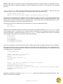
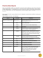
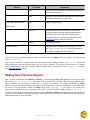
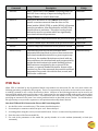
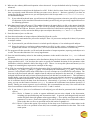
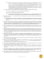
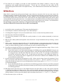
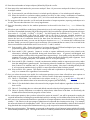
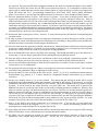
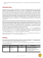
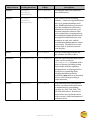
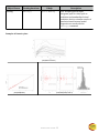
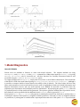
Pmetrics User Manual November 21, 2011 Package Version 0.17 An R package for parametric and non-‐ parametric modeling and simula6on of pharmacokine6c and pharmacodynamic systems Table of Contents Introduc6on ...................................................................................................................................................3 Disclaimer ......................................................................................................................................................3 System Requirements and Installa6on ...........................................................................................................3 What This Manual Is Not ................................................................................................................................3 Pmetrics Components ....................................................................................................................................4 General Workflow ..........................................................................................................................................5 Pmetrics Input Files ........................................................................................................................................6 Data .csv Files .........................................................................................................................................................6 Model .for Files .......................................................................................................................................................7 Subrou'ne 1: DIFFEQ ........................................................................................................................................7 Subrou'ne 2: OUTPUT .......................................................................................................................................8 Subrou'ne 3: SYMBOL ......................................................................................................................................8 Subrou'ne 4: GETFA .........................................................................................................................................9 Subrou'ne 5: GETIX ..........................................................................................................................................9 Subrou'ne 6: GETTLAG .....................................................................................................................................9 Subrou'ne 7: ANAL3 .......................................................................................................................................10 How to use R and Pmetrics ..........................................................................................................................10 Pmetrics Data Objects ..................................................................................................................................12 Making New Pmetrics Objects ......................................................................................................................14 IT2B Runs .....................................................................................................................................................15 NPAG Runs ..................................................................................................................................................18 Simulator Runs .............................................................................................................................................21 PloXng ........................................................................................................................................................21 Model Diagnos6cs ........................................................................................................................................25 Internal Valida6on ................................................................................................................................................25 External Valida6on ...............................................................................................................................................26 References ...................................................................................................................................................27 Pmetrics User’s Guide 2 Introduction Thank you for your interest in Pmetrics! This guide provides instructions and examples to assist users of the Pmetrics R package, by the Laboratory of Applied Pharmacokinetics at the University of Southern California. Please see our website at www.lapk.org for more information. Here are some tips for using this guide. • Items that are hyperlinked can be selected to jump rapidly to relevant sections. • At the bottom of every page, the text “Pmetrics User’s Guide” can be selected to jump immediately to the table of contents. • Items in courier font correspond to R commands Disclaimer You, the user, assume all responsibility for acting on the results obtained from Pmetrics. The USC Laboratory of Applied Pharmacokinetics, members and consultants to the Laboratory of Applied Pharmacokinetics, and the University of Southern California and its employees assume no liability whatsoever. Your use of the package constitutes your agreement to this provision. System Requirements and Installation Pmetrics is a package for the freely available statistical and programming R software, which can be obtained from http://www.R-‐project.org/. R and Pmetrics run in Windows and Mac (Unix) environments. In order to run Pmetrics, a Fortran compiler is required. The freely available gfortran compiler is available for Mac and Windows users. For Mac users: Link to http://gcc.gnu.org/wiki/GFortranBinaries, click the MacOS link under “Binaries available for gfortran” at the top of the page. Select the appropriate source to download, based on your system. For Windows users: Link to http://tdm-‐gcc.tdragon.net/download and select the installer download link at the very top. Once you launch the downloaded installer, accept all the defaults EXCEPT BE SURE to choose fortran under the components dialog window JUST BEFORE YOU CLICK INSTALL. Do this by selecting the “+” next to “gcc” at the top of the list, and then scrolling down to check the fortran box. If you don’t do this, you will not get gfortran by default. A text editor that can link to R is useful for saving scripts. Both the Windows and Mac versions of R have rudimentary text editors that are stable and reliable. Numerous other free and paid editors can also do the job, and these can be located by searching the internet. We prefer Rstudio which is available for Mac and Windows, and is free. We have also used the freely available Komodo with the SciViews-‐K add-‐on, although it is somewhat dif_icult to set up proper communication with R. Once working, however, it is an intuitive and easy, yet powerful, scripting environment. Email us if you need help at [email protected]. Pmetrics is currently distributed as a source _ile. To install Pmetrics from the R console, use the command install.packages(file.choose()), and navigate when prompted to the folder in which you placed the Pmetrics .tar.gz source _ile. Pmetrics will need the following packages for some functions: chron, rgl, and R2HTML. However, you do not have to install these if you do not already have them in your R library. They should automatically be downloaded and installed the _irst time you use a Pmetrics function that requires them, but if something goes awry (such as no internet connection or busy server) you can do this manually. What This Manual Is Not We assume that the user has familiarity with population modeling and R, and thus this manual is not a tutorial for basic concepts and techniques in either domain. We have tried to make the R code simple, regular and well documented. A very good free online resource for learning the basics of R can be found at http:// Pmetrics User’s Guide 3 www.statmethods.net/index.html. We recognize that initial use of a new software package can be complex, so please feel free to contact us at any time: [email protected]. This manual is also not intended to be a theoretical treatise on the algorithms used in IT2B or NPAG. For that the user is directed to our website at www.lapk.org. Pmetrics Components There are three main software programs that Pmetrics controls. • IT2B is the ITerative 2-‐stage Bayesian parametric population PK modeling program. It is generally used to estimate parameter ranges to pass to NPAG. It will estimate values for population model parameters under the assumption that the underlying distributions of those values are normal or transformed to normal. • NPAG is the Non-‐parametric Adaptive Grid software. It will create a non-‐parametric population model consisting of discrete support points, each with a set of estimates for all parameters in the model plus an associated probability (weight) of that set of estimates. There can be at most one point for each subject in the study population. There is no need for any assumption about the underlying distribution of model parameter values. • The simulator is a semi-‐parametric Monte Carlo simulation software program that can use the output of IT2B or NPAG to build randomly generated response pro_iles (e.g. time-‐concentration curves) for a given population model, parameter estimates, and data input. Simulation from a non-‐parametric joint density model, i.e. NPAG output, is possible, with each point serving as the mean of a multivariate normal distribution, weighted according to the weight of the point. The covariance matrix of the entire set of support points is divided equally among the points for the purposes of simulation. Pmetrics has groups of R functions named logically to run each of these programs and to extract the output. These are extensively documented within R by using the help(command) or ?command syntax. • ITrun, ITparse, ITload, ITreport, ERRrun • NPrun, NPparse, NPload, NPreport • SIMrun, SIMparse For IT2B and NPAG, the “run” functions generate batch _iles, which when executed, launch the software programs to do the analysis. ERRrun is a special implementation of IT2B designed to estimate the assay error polynomial coef_icients from the data, when they cannot be calculated from assay validation data (using makeErrorPoly()) supplied by the analytical laboratory. The batch _iles contain all the information necessary to complete a run, tidy the output into a date/time stamped directory with meaningful subdirectories, extract the information, generate a report, and a saved RData _ile of parsed output which can be quickly and easily loaded into R. On Mac (Unix) systems, the batch _ile will automatically launch in a Terminal window. On Windows systems, the batch _ile must be launched manually. In both cases, the execution of the program to do the actual model parameter estimation is independent of R, so that the user is free to use R for other purposes. For the Simulator, the “run” function will execute the program directly within R. For all programs, the “parse” functions will extract the primary output from the program into meaningful R data objects. For IT2B and NPAG, this is done automatically at the end of a successful run, and the objects are saved in the output subdirectory as IT2Bout.Rdata or NPAGout.Rdata, respectively. For IT2B and NPAG, the “load” functions can be used to load the above .Rdata _iles after a successful run. The “report” functions are automatically run at the end of a successful run, and these will generate an HTML page with summaries of the run, as well as the .Rdata _iles and other objects. The default browser will be automatically launched for viewing of the HTML report page. Within Pmetrics there are also functions to manipulate data .csv _iles and process and plot extracted data. • Manipulate data .csv _iles: PMreadMatrix, PMcheckMatrix, PMwriteMatrix, PMmatrixRelTime, PMwrk2csv • Process data: makeAUC, makeCov, makeCycle, makeFinal, makeOP, makeErrorPoly Pmetrics User’s Guide 4 • Plot data: plot.PMcov, plot.PMcycle, plot.PM_inal, plot.PMmatrix, plot.PMop, plot.PMsim • Model selection and diagnostics: PMcompare, plot.PMop (with residual option), PMdiag Again, all functions have extensive help _iles and examples which can be examined in R by using the help(command) or ?command syntax. General Workflow The general Pmetrics work_low for IT2B and NPAG is shown in the diagram below. Data .csv file u ITr n( n Pru ,) N Model .for file () PreparaFon program InstrucFon file Engine program IT lo ad o Pl N (), ad () Output R is used to specify the working directory containing the data .csv and model .for _iles, and possibly an instruction _ile if IT2B or NPAG have been run previously. Through the batch _ile generated by R, the preparation program is compiled and executed. If this is the _irst run, the user will answer several questions about the run, supplying necessary information. This information can be saved as an instruction _ile for future runs. The batch _ile will then compile and execute the engine _ile, which will generate several output _iles upon completion. Finally, the batch _ile will call the R script to generate the summary report and several data objects, including the IT2Bout.Rdata or NPAGout.Rdata _iles which can be loaded into R subsequently using ITload() or NPload(). On subsequent runs, the user may specify the name of the instruction _ile as an argument to ITrun() or NPrun(). This will result in fully automated execution, with no further input from the user required. All input _iles (data, model, and instruction) are text _iles which can be edited directly by advanced users. Pmetrics User’s Guide 5 Pmetrics Input Files Data .csv Files Pmetrics accepts input as a spreadsheet “matrix” format. It is designed for input of multiple records in a concise way. Files are in comma-‐separated-‐values (.csv) format. Examples of programs that can save .csv _iles are any text editor (e.g. TextEdit on Mac, Notepad on Windows) or spreadsheet program (e.g. Excel). Click on hyperlinked items to see an explanation. IMPORTANT: The order, capitalization and names of the header and the _irst 12 columns are _ixed. All entries must be numeric, with the exception of ID and “.” for non-‐required placeholder entries. POPDATA APR_11 #ID EVID TIME DUR DOSE INPUT OUT OUTEQ GH GH GH GH GH GH GH GH 1423 1423 1423 1423 1423 0 . . . . 0.5 . . 0 0 . . . 400 . . . . 150 . . 400 100 . . . 1 . . . . 1 . . 1 2 . . . . 1 1 1 . . 1 1 . . 1 1 2 1 0 0 0 4 1 0 0 1 1 0 0 0 0 0.5 1 2 0 3.5 5.12 24 0 0.1 1 2 2 . 0.42 0.46 2.47 . . 0.55 0.52 . . -‐99 0.38 1.6 C0 . 0.01 0.01 0.01 . 0.01 0.01 0.01 . . 0.01 0.01 0.05 C1 . 0.1 0.1 0.1 . 0.1 0.1 0.1 . . 0.1 0.1 0.2 C2 . 0 0 0 . 0 0 0 . . 0 0 -‐0.11 C3 COV… . 0 0 0 . 0 0 0 . . 0 0 0.002 POPDATA APR_11 This is the header for the _ile and must be in the _irst line. It identi_ies the version. #ID This _ield must be preceded by the “#” symbol to con_irm that this is the header row. It can be numeric or character and identi_ies each individual. All rows must contain an ID, and all records from one individual must be contiguous. Any subsequent row that begins with “#” will be ignored, which is helpful if you want to exclude data from the analysis, but preserve the integrity of the original dataset, or to add comment lines. IDs should be 11 characters or less but may be any alphanumeric combination. There can be at most 800 subjects per run. EVID This is the event ID _ield. It can be 0, 1, or 4. Every row must have an entry. 0 = observation 1 = input (e.g. dose) 2, 3 are currently unused 4 = reset, where all compartment values are set to 0 and the time counter is reset to 0. This is useful when an individual has multiple sampling episodes that are widely spaced in time with no new information gathered. TIME This is the elapsed time in decimal hours since the _irst event. It is not currently clock time (e.g. 21:30), although this is planned. Every row must have an entry, and within a given ID, rows must be sorted chronologically, earliest to latest. DUR This is the duration of an infusion in hours. If EVID=1, there must be an entry, otherwise it is ignored. For a bolus (i.e. an oral dose), set the value equal to 0. Pmetrics User’s Guide 6 DOSE This is the dose amount. If EVID=1, there must be an entry, otherwise it is ignored. INPUT This de_ines which input (i.e. drug) the DOSE corresponds to. Inputs are de_ined in the model _ile. OUT This is the observation, or output value. If EVID=0, there must be an entry; if missing, this must be coded as -‐99. It will be ignored for any other EVID and therefore can be “.”. There can be at most 150 observations for a given subject. OUTEQ This is the output equation number that corresponds to the OUT value. Output equations are de_ined in the model _ile. C0, C1, C2, C3 These are the coef_icients for the assay error polynomial for that observation. Each subject may have up to one set of coef_icients per output equation. If more than one set is detected for a given subject and output equation, the last set will be used. If there are no available coef_icients, these cells may be left blank or _illed with “.” as a placeholder. COV... Any column after the assay error coef_icients is assumed to be a covariate, one column per covariate. Model .for Files Model _iles for Pmetrics are Fortran text _iles. The current version is TSMULTI. The safest thing to do is to edit old versions of the model _iles to make new versions. Fortran is very fussy when it comes to spacing; one column off can result in a failed run. There are seven subroutines that can be modi_ied by the user, all by writing simple Fortran code. Model _iles have comment lines to indicate where user code should go. Subrou6ne 1: DIFFEQ In this subroutine, users specify the differential equations that de_ine the model. There can be a maximum of 20 such equations. All parameters, unless secondarily de_ined, are referred to as P(x) where x is the number of the variable. The parameters are assigned in subroutine SYMBOL. An example of differential equations follows. XP(1) = -P(1)*X(1) XP(2) = P(1)*X(1) - P(2)*X(2) XP is the Fortran notation for dx/dt, P(1) is parameter 1, and X(1) is the amount in compartment 1. Alternatively, one could specify more meaningful parameter names and secondary equations, as shown below. XKA = DEXP(P(1)) XKEL = DEXP(P(2)) / (CV(1)/70)**0.25 XP(1) = -XKA*X(1) XP(2) = RATEIV(1) + XKA*X(1) - XKEL*X(2) DEXP is the Fortran code for double precision e(...), and in this example, P(1) etc. are the natural logs of the variables. Note that all variables are implicitly declared to be REAL *8 in Pmetrics model _iles. Variables cannot start with the letters I through N, as these are reserved; hence the XKA notation. CV(1) is the notation to de_ine the value of covariate 1, as de_ined in the data .csv _ile. It will refer to the values contained in the _irst column after the C3 entry. Of course, CV(2), CV(3), etc. can be used if these columns are de_ined in the data. Note that any covariate relationship to any parameter may be described as the user wishes by mathematical equations and Fortran code, allowing for exploration of complex, non-‐linear, time-‐dependent, and/or conditional relationships. Pmetrics User’s Guide 7 RATEIV(1) is the notation to indicate an infusion of input 1 (typically drug 1). The duration of the infusion and total dose is de_ined in the data .csv _ile. Up to 7 inputs are currently allowed. These can be used in the model _ile as RATEIV(1), RATEIV(2), etc. The compartments for receiving the inputs of oral (bolus) doses are de_ined in subroutine SYMBOL. This is a simple example, which does not actually require differential equations in Pmetrics, as we shall see. However, it gives the idea of how to specify a model. Subrou6ne 2: OUTPUT In this subroutine, users specify the equations that de_ine the outputs of the model. As for DIFFEQ, all variables, unless secondarily de_ined, are referred to as P(x) where x is the number of the variable. The variables are assigned in subroutine SYMBOL. An example of an output equation follows. Y(1) = X(2)/P(3) Y(1) is the Fortran notation for Output 1. Alternatively, one could specify more meaningful parameter names and secondary equations. V = DEXP(P(3))*CV(1) Y(1) = X(2)/V Since V does not start with the letters I through N, it is an acceptable variable name. CV(1) is the same as de_ined before: the value of covariate 1 at the appropriate time, as speci_ied in the data .csv _ile. There can be a maximum of 6 outputs. They are referred to as Y(1), Y(2), etc. Subrou6ne 3: SYMBOL In this subroutine, there are up to three areas which need attention from the user. In the _irst section, the user can de_ine compartments that will receive bolus doses. By default, these compartments correspond to the input number, so that compartment 1 will receive input 1, etc. This can be reassigned using the syntax: NBCOMP(1) = 2 which assigns compartment 2 to receive any bolus doses from input 1. A dose is de_ined as a bolus in a data .csv _ile by setting duration to 0. Any value greater than 0 implies an infusion, which serves as an input as de_ined in the DIFFEQ subroutine. In the second section of SYMBOL , the user speci_ies the number of compartments in the model. This can be one of three kinds: 1. A positive integer equal to the number of XP(.) equations in DIFFEQ. This will instruct Pmetrics to use the ordinary differential equation solver to _it the model to the data. 2. Zero. This implies that the model is de_ined as an analytic equation or equations in OUTPUT. 3. -‐1, which tells Pmetrics to use analytic equations as de_ined in the subroutine ANAL3. In this case, any differential equations in DIFFEQ are ignored. As an example: N=2 which corresponds to the number of differential equations in DIFFEQ above. Again, N cannot be greater than 20. This statement must start in column 8. The third section of SYMBOL is for de_ining the random and _ixed variable names in the model. It is headed by a statement declaring the number of variables, followed by the variable names. Pmetrics User’s Guide 8 NP=3 PSYM(1)='Ka' PSYM(2)='Kel' PSYM(3)='Vol' Note the use of single quotes. Variable names must be no greater than 11 characters and not contain any spaces. These statements must also begin in column 8. The number of parameters must be between 2 and 32, with at most 30 random or 20 Jixed. Subrou6ne 4: GETFA In this subroutine, users can specify which parameter, if any, is to be _itted as the bioavailability (FA) of a given input. By default, all inputs have an FA=1. The syntax is as follows. FA(1)=P(4) Now the FA for input 1 is assigned to variable 4. Of course secondary expressions are also permissible. FA(3)=DEXP(P(7))*CV(3) Here FA for input 3 is assigned to the product of eP(7) and CV(3). CV(3) might be a covariate that speci_ies gastric pH, for example. Subrou6ne 5: GETIX In this subroutine, users can specify the initial conditions of a given compartment. By default, all compartments are set to X(.)=0. The syntax is as follows. X(1)=P(4) X(2)=CV(4)*P(3) In the _irst case, the initial condition for compartment 1 becomes another variable, P(4), to _it in the model, given the observed data. In the second case, the initial condition for compartment 2 becomes the value of covariate 4 multiplied by the current estimate of P(3) during each iteration. This is useful when a subject has been taking a drug as an outpatient, and comes in to the lab for PK sampling, with measurement of a concentration immediately prior to a witnessed dose, which is in turn followed by more sampling. In this case, CV(4) or any other covariate can be set to the initial measured concentration, and if P(3) is the volume of compartment 2, the initial condition (amount) in compartment 2 will now be set to the measured concentration of drug multiplied by the estimated volume for each iteration until convergence. Subrou6ne 6: GETTLAG In this subroutine, users can specify a variable to be _itted as the lag time for a given input. By default, all lag times are set to 0. The syntax is as follows. TLAG(1)=P(4) TLAG(2)=DEXP(P(4))*CV(3) In the _irst case, the lag time for input 1 becomes another variable, P(4), to _it in the model, given the observed data. In the second case, the lag time for input 2 becomes the exponentiated value of P(4) Pmetrics User’s Guide 9 multiplied by the third covariate speci_ied in the data .csv _ile, for example an indicator of 1 if capsule, 0 if liquid. Subrou6ne 7: ANAL3 If N=-1 in SYMBOL, users can specify equations which can be used to estimate parameter values without the use of differential equations (analytical models), speeding up run times 10,000 fold. Equations are de_ined for three basic models: 1) one compartment; 2) one dosing and one central compartment; and 3) one dosing, one central and one peripheral compartment. The parameters are formulated as KA, KE, KCP, KPC, and V, which cannot be changed. However, any secondary equations that de_ine these primary variables are permissible. KA = DEXP(P(1)) KE = DEXP(P(2)) / (CV(1)/70)**0.25 KCP = 0 KPC = 0 V = DEXP(P(5))*(CV(1)/70) This speci_ies a model with an absorptive compartment, elimination from a central compartment scaled allometrically to normalized body weight (if this is the value of the _irst covariate), no peripheral compartment (by setting KCP and KPC to 0), and volume scaled to normalized body weight. All parameters in this example are log transformed, so must be exponentiated in the model For users who prefer parameterization in terms of clearances, if P(1) is assigned to CL and P(2) is VOL, then by the relationship K = CL / VOL, you may specify: KE = P(1) / P(2) All other parameters, including fraction absorbed (GETFA), initial conditions (GETIX) and lag times (GETTLAG) are also permissible with analytical models. As for differential equation models, any covariate relationship to any parameter may be described as the user wishes by mathematical equations and Fortran code, allowing for exploration of complex, non-‐linear, time-‐dependent, and/or conditional relationships. How to use R and Pmetrics The _irst thing to do is to ensure that appropriate Pmetrics model .for and data .csv _iles are in the working directory. R can be used to help prepare the data .csv _ile by importing and manipulating spreadsheets (e.g. read.csv()). The Pmetrics function PMcheckMatrix() can be used to check an R dataframe that is to be saved as a Pmetrics data .csv _ile for errors. The function PMwriteMatrix() can be used to write the R data object in the correct format for use by IT2B, NPAG, or the Simulator. If this is a _irst-‐time run, the R commands to run IT2B or NPAG are as follows. Recall that the “#” character is a comment character. library(Pmetrics) setwd(“working directory”) NPrun() #for NPAG #or ITrun() for IT2B The _irst line will load the Pmetrics library of functions. The second line sets the working directory to the speci_ied path. The third line generates the batch _ile to run NPAG or IT2B and saves it to the working directory. If this is the very _irst time ever to run NPAG or IT2B, the user will be _irst prompted in R to specify the Fortran compiler in use. Pmetrics User’s Guide 10 NOTE: On Mac systems, the batch _ile will be automatically launched in a Terminal window. On Windows systems, the batch _ile must be launched manually by double clicking the np_run.bat or it_run.bat _ile in the working directory. ITrun() and NPrun() both return the full path of the output directory to the clipboard. Therefore, the next command to enter in the script will change the working directory to this output directory. setwd(“output directory”) #paste the directory name between the double quotation marks This cannot be executed until the completion of the run when the subdirectory tree is constructed by the batch _ile (as described in R documentation for NPrun or ITrun) and the run output is sorted to the appropriate folders. This subdirectory tree will be contained in the working directory. A folder with a date-‐ and time-‐stamped name will be created, with subdirectories for input, output and other _iles. Now the output of IT2B or NPAG needs to be loaded into R, so the next command does this. NPload() #or ITload() Details of these commands and what is loaded are described in the R documentation (?NPload or ?ITload) and in the following section. An integer can be included within the parentheses to be appended to the names of loaded R objects, allowing for comparison between runs, e.g. NPload(1). Finally, at this point other Pmetrics commands can be added to the script to process the data, such as the following. plot(final) plot(cycle) plot(op$pop1) plot(op$post1) plot(op$pop1,resid=T) plot(op$post1,resid=T) Of course, the full power of R can be used in scripts to analyze data, but these simple statements serve as examples. We suggest that the R script for a particular project be saved into a folder called “Rscript” in the working directory. Folders are not be moved by the batch _ile. Within the script, number runs sequentially and use comments liberally to distinguish runs, as shown below. library(Pmetrics) #Run 1 - Ka, Kel, V, all subjects setwd(“working directory”) NPrun() setwd(“output directory 1”) NPload(1) ... #Run 2 - Ka, Kel, V, allometric scaling, all subjects setwd(“working directory”) NPrun(model=”model2.for”,instr=”file”) #assumes an appropriate instruction file from a earlier run, possibly edited setwd(“output directory 2”) NPload(2) ... Remember in R that the command example(function) will provide examples for the speci_ied function. Most Pmetrics functions have examples. Pmetrics User’s Guide 11 Pmetrics Data Objects After a successful IT2B or NPAG run, an R data_ile is saved in the output subdirectory of the newly created, time and date-‐stamped folder in the working directory. After IT2B, this _ile is called “IT2Bout.Rdata”, and after NPAG it is called “NPAGout.Rdata”. As mentioned in the previous section, these data _iles can be loaded by ensuring that the correct output folder is set as the working directory, and then using the Pmetrics commands ITload() or NPload(). Both commands load their respective Rdata _iles into R, making the contained objects available for plotting and other analysis. Objects loaded by ITload() and NPload() Objects op (class: PMop,data.frame) _inal (class: PM_inal,list) Variables Comments $pop1, $post1, ... Population and posterior predictions for each output equation, i.e. 1, 2, ... $id Subject identi_ication $time Observation time in relative decimal hours $obs Observation $pred Prediction based on median of population or posterior parameter value distributions $block Dosing block, usually 1 unless data _ile contains EVID=4 dose reset events, in which case each such reset within a given ID will increment the dosing block by 1 for that ID $obsSD Calculated standard deviation (error) of the observation based on the assay error polynomial $d Difference between pred and obs $ds Squared difference between pred and obs $wd $d, weighted by the $obsSD $wds $ds, weighted by the $obsSD $popPoints (NPAG only) Data.frame of the _inal cycle joint population density of grid points with column names equal to the name of each random parameter plus $prob for the associated probability of that point Pmetrics User’s Guide 12 Objects cycle (class: PMcycle, list) Variables Comments $popMean The _inal cycle mean for each random parameter distribution $popSD The _inal cycle standard deviation for each random parameter distribution $popCV The _inal cycle coef_icient of variation for each random parameter distribution $popVar The _inal cycle variance for each random parameter distribution $popCov The _inal cycle covariance matrix for each random parameter distribution $popCor The _inal cycle correlation matrix for each random parameter distribution $popMedian The _inal cycle median for each random parameter distribution $gridpts (NPAG only) The initial number of support points $ab Matrix of boundaries for random parameter values. For NPAG, this is speci_ied by the user prior to the run; for IT2B, it is calculated as a user speci_ied multiple of the SD for the parameter value distribution $names Vector of names of the random parameters $ll Matrix of cycle number and -‐2*Log-‐likelihood at each cycle $gamlam A matrix of cycle number and gamma or lambda at each cycle (see item #16 under NPAG Runs below for a discussion of gamma and lambda) $mean A matrix of cycle number and the mean of each random parameter at each cycle, normalized to initial mean $sd A matrix of cycle number and the standard deviation of each random parameter at each cycle, normalized to initial standard deviation $median A matrix of cycle number and the median of each random parameter at each cycle, normalized to initial standard deviation Pmetrics User’s Guide 13 Objects post (class: data.frame) Variables Comments $aic A matrix of cycle number and Akaike Information Criterion at each cycle $bic A matrix of cycle number and Bayesian (Schwartz) Information Criterion at each cycle $id Subject identi_ication $pred1, ... Bayesian posterior predictions for each output equation, based on mean, median, and mode, as speci_ied by the user and with frequency also speci_ied by the user in the run instructions (see NPAG Runs below, items 23 and 24). $block See op$block above NPAG only NPdata, ITdata Raw data used to make the above objects. Please use ?NPparse or ?ITparse in R for discussion of the data contained in these objects Since R is an object oriented language, to access the observations in a PMop object, for example, use the following syntax: op$post1$obs. Note that you can place an integer within the parentheses of the loading functions, e.g. NPload(1), which will suf_ix all the above objects with that integer, e.g. op.1, _inal.1, NPdata.1. This allows several models to be loaded into R simultaneously, each with a unique suf_ix, and which can be compared with the PMcompare() command (see Model Diagnostics below). Making New Pmetrics Objects Once you have loaded the raw (NPdata or ITdata) or processed (op, Jinal, cycle, post) data objects described above with NPload() or ITload(), should you wish to remake the processed objects with parameters other than the defaults, you can easily do so with the make family of commands. For example, the default for PMop objects is to use the prediction based on the median of the population or posterior distribution. If you wish to use the mean of the distribution, remake the PMop object using makeOP(). If you wish to see all the cycle information in a PMcycle object, not omitting the _irst 10% of cycles by default, remake it using makeCycle(). For all of the following commands, the data input is either NPdata or ITdata, with additional function arguments speci_ic to each command. Accessing the help for each function in R will provide further details on the arguments, defaults and output of each command. Pmetrics User’s Guide 14 Command Description R help makeAUC Make a data.frame of class PMauc containing subject ID and AUC from a variety of inputs including objects of PMop, PMsim or a suitable data.frame makeCov Generate a data.frame of class PMcov with subject-‐ ?makeCov speci_ic covariates extracted from the data .csv _ile, mean/median (NPAG/IT2B) or mode (NPAG) of Bayesian posterior parameter value distributions, and AUC from speci_ied start to end times. This object can be plotted and used to test for covariates which are signi_icantly associated with model parameters. makeCycle Create a PMcycle object described in the previous section. ?makeCycle makeFinal Create a PM_inal object described in the previous section. ?makeFinal makeOP Create a PMop object described in the previous section. ?makeOP makeErrorPoly This function plots _irst, second, and third order polynomial functions _itted to pairs of observations and associated standard deviations for a given output assay. In this way, the standard deviation associated with any observation may be calculated and used to appropriately weight that observation in the model building process. Observations are weighted by the reciprocal of the variance, or squared standard deviation. Output of the function is a plot of the measured observations and _itted polynomial curves and a list with the _irst, second, and third order coef_icients. ?makeErrorPoly ?makeAUC IT2B Runs When IT2B is launched by the R-‐generated batch script without an instruction _ile, the user must answer the following questions, prompted by the program. There is an opportunity at the end to review and correct answers, so making a mistake is not a reason necessarily to abort. Answers to the following questions can be saved in an instruction _ile which can be used for future runs. Instruction _iles are simply text _iles with speci_ic entries which can be modi_ied directly by advanced users. Less advanced users can initiate an IT2B run from Pmetrics without specifying an instruction _ile (even if one exists), and then load it as described in item 7 below. You will then have the opportunity to see previous responses to each question and modify them if desired. Note that IT2B and NPAG instruction Jiles are NOT interchangeable. 1. Are the _iles in the current directory? The answer should always be 1. 2. Do an analysis or examine results from prior run? Almost always 1. 3. A warning about using the correct/current model format. Press 1 or some other key and then return. 4. Enter the name of the Fortran model _ile. 5. For each of the parameters in the model _ile, specify whether it is to be random (estimated) or _ixed (not estimated). Pmetrics User’s Guide 15 6. What are the ordinary differential equation solver tolerances? Accept the default value by choosing 1, unless advanced. 7. Are the instructions coming from the keyboard or a _ile? If this is the _irst time, choose 0 for keyboard. If you have a previously saved instruction _ile that you want to use, choose 1. However, typically if you have an instruction _ile that you want to use, you will specify this in the R script with ITrun(instr=“filename”) for automated analysis. 7.1. If you selected keyboard input, you will answer the following questions, otherwise you will be prompted for the name of your instruction _ile and once loaded, you will verify your previously supplied answers to the following questions. 8. What data input format will you use? The standard format is the matrix block .csv _ile, so the answer should be 1. Working copy _iles are an older format. The .csv _ile is actually converted to these .wrk _iles, one _ile per subject, prior to an IT2B run. However, some function will be lost in the Pmetrics package by using .wrk input directly without a .csv _ile, such as the ability to plot raw subject data via the plot.PMmatrix() function. 9. Enter the name of your .csv _ile now. 10. Enter the total number of unique subjects (de_ined by ID) in the .csv _ile. 11. How many of the total number do you want to analyze? Enter 1 if you want to analyze all of them, 0 if you want to analyze a subset. 11.1. If you entered 0, you will then choose 1 to include speci_ic subjects, or 2 to exclude speci_ic subjects. 11.2. Enter the inclusion or exclusion subject numbers (not IDs) in order, using a combination of numbers, hyphens and commas. For example: 1,3-‐5,7,10. Press return and then enter 0 to conclude entry. 12. The program will then open the .csv _ile and read the number of output equations, reporting each subject as it is read. This can take some time if it is a very large dataset. 13. Enter the initial boundary values for the random parameters in the model in the form “min, max” followed by return. 14. The estimated mean for each parameter value distribution during the _irst iteration will be the median of the range speci_ied in #13. You now have the option to specify the standard deviation for the parameter value distribution, which by default is half of the range in #13. Choose 1 to accept this (the usual answer) or 0 to change it to something else, expressed as a multiple of the range. 15. In IT2B, the standard deviation (SD) of the observation [obs] is modeled by a polynomial equation with up to four terms: C0 + C1*[obs] + C2*[obs]2 + C3*[obs]3. You will specify the coef_icients C0, C1, C2 and C3. You can now choose 1 if every subject has the same coef_icients or 0 to use a unique set of coef_icients for each subject. The _irst case is the more usual, when all samples from all subjects are analyzed in the same lab. If samples are analyzed in different labs and you have the assay data from each lab then you would enter 0. This information should ideally come from the analytic lab in the form of inter-‐run standard deviations or coef_icients of variation at standard concentrations. You can use the Pmetrics function PMerrorPoly() to choose the best set of coef_icients that _it the data from the laboratory. Alternatively, if you have no information about the assay, you can use the Pmetrics function ERRrun() to estimate the coef_icients from the data (see #15.1.3 below). Finally, you can use a generic set of coef_icients. We recommend that as a start, C0 be set to half of the lowest concentration in the dataset and C1 be set to 0.15. C2 and C3 can be 0. 15.1. If you choose 1 (one set of coef_icients for all subjects) you will then be presented with 3 additional choices. 15.1.1. Choice 1: Gamma is a scalar to capture additional process noise related to the observation, including mis-‐speci_ied dosing and observation times. In general, well-‐designed and executed studies will have data with gamma values approaching 1. Poor quality, noisy data will result in gammas of 5 or more. Choose this option if you wish to _ix the assay error coef_icients to values either in the data .csv _ile or as speci_ied in item #16, and to _ix gamma to 1. 15.1.2. Choice 2: Choose this option if you wish to _ix the assay error coef_icients to values either in the data .csv _ile or as speci_ied in item #16, but to estimate gamma based on the data. This is the usual option. Pmetrics User’s Guide 16 15.1.3. Choice 3: Choose this option if you wish to estimate the assay error coef_icients based on your data for use in future runs. Although you can access this option by using either ITrun() or ERRrun() in R, the instruction _iles that you save and the generated output _iles will be different. Therefore, we recommend that if you intend to choose this option, use ERRrun() in R, which will generate an ASS0001 _ile that contains the estimates for C0, C1, C2, and C3. You can then include this _ile in the working directory (along with a model .for _ile and a data .csv _ile) to do an IT2B run, supplying the _ile name in #16.1 below. 15.2. If you choose 0 (unique coef_icients for each subject), you will be presented with two choices. 15.2.1. Choice 1: Fix gamma to 1. See the discussion above in #15.1.1. 15.2.2. Choice 2: Estimate gamma based on the data. 15.2.3. You now need to specify where to obtain the values for C0, C1, C2, C3 , either from the data .csv _ile and from the entry in #16 (Choice 1), or on an individual basis during the IT2B run1 (Choice 0). 16. Enter the values for C0, C1, C2, C3 that will be used for all patients who do not have values associated with them in the data .csv _ile. 16.1. You have the option of entering a _ile name that contains the output of a previous estimation generated by choosing 3 in #15.1.3 above. Usually this _ile will be called ASS0001 and it must be in the working directory. 17. After assay error pattern and estimates are speci_ied for all output equations, enter the salt fraction of the drug, usually 1. Salt fraction is the percentage of administered compound that contains active drug. For example, the mean salt fraction for theophylline is 0.85. This is not the same as bioavailability, which is the fraction of drug absorbed after non-‐parenteral administration (e.g. oral) compared to intravenous administration. 18. Enter the convergence criterion. When the difference between log-‐likelihoods of successive iterations is less than or equal to this criterion, IT2B will converge and terminate. The default is 0.001, which is the typical response. 19. Enter the maximum number of cycles. This can be 1 to 41000, and IT2B will terminate at convergence or the number of cycles you specify here, whichever comes _irst. Early in model exploration values of 10 to 100 can be useful, with larger values such as 1000 later in model development. In order to facilitate model comparison, however, we recommend using the same cycle limit for all early models, e.g. 100, rather than choosing 10 for one and 100 for another. 20. IT2B can pass parameter ranges to NPAG via a FROMxxxx (usually FROM0001) _ile. The default ranges to be used in NPAG are 5 times the _inal IT2B cycle standard deviation above and below the _inal cycle mean. If your parameters are normally distributed, 5 is a typical number. For log-‐normally distributed parameters, 3 is a better choice. 21. You are now offered the opportunity to check all of your entries for correctness. Choose 1 each time to indicate correct entries, or 0 to change them. 22. Enter 1 if you wish to save all the instructions in an instruction _ile. If you do this, you can specify this instruction _ile in Pmetrics by using the ITrun(instr=“filename”) option, and including “_ilename” in the working directory with the model .for _ile and the data .csv _ile. 23. The program will cycle through your subject records again to extract all relevant information. This can take some time if the population is large or individual records are long. 24. Specify the nature of each covariate in the data .csv _ile. Enter 1 if it is to be considered constant between measurements (e.g. gender) or 2 if values should be extrapolated between observations (e.g. creatinine clearance). 25. If you chose unique assay error coef_icients for each subject in #15 above, you will now specify whether you wish to use coef_icients found in the data .csv _ile (choice 1), the general coef_icients speci_ied in #16 above (choice 2), or a different set that you enter manually now (choice 0) in the form C0, C1, C2, C3. 26. Some output will print to the terminal window which contains information that you can ignore while running IT2B from Pmetrics. Press 1 followed by return to begin the IT2B analysis. Pmetrics User’s Guide 17 27. The IT2B run can complete in seconds for small populations with analytic solutions, or days for large populations with complex differential equations. At the end of a successful run, the results will be automatically parsed and saved to the output directory. Your default browser will launch with a summary of the run. NPAG Runs When NPAG is launched by the R-‐generated batch script without an instruction _ile, the user must answer the following questions, prompted by the program. There is an opportunity at the end to review and correct answers, so making a mistake is not a reason necessarily to abort. Answers to the following questions can be saved in an instruction _ile which can be used for future runs. Instruction _iles are simply text _iles with speci_ic entries which can be modi_ied directly by advanced users. Less advanced users can initiate an NPAG run from Pmetrics without specifying an instruction _ile (even if one exists), and then load it as described in item 7 below. You will then have the opportunity to see previous responses to each question and modify them if desired. Note that IT2B and NPAG instruction Jiles are NOT interchangeable. 1. Are the _iles in the current directory? The answer should always be 1. 2. Do an analysis or examine results from prior run? Almost always 1. 3. A warning about using the correct/current model format. Press 1 or some other key and then return. 4. Enter the name of the Fortran model _ile. 5. For each of the parameters in the model _ile, specify whether it is to be random (estimated) or _ixed (not estimated). 6. What are the ordinary differential equation solver tolerances? Accept the default value by choosing 1, unless advanced. 7. NPAG creates a temporary instruction _ile in case something happens, so that instructions entered to date can be recovered. Accept the default by choosing 1. You can save with a meaningful _ilename later. If it already exists, you will be asked if you wish to overwrite the _ile, which is usually the thing to do. 8. If you have previously run IT2B, you can automatically import the suggested parameter ranges. Choose 1 to do this, and 0 to run NPAG without a previous IT2B run. 8.1. If you choose option 1, you must specify the name of a FROMxxxx _ile, typically FROM0001 that you can _ind in an output directory after a successful IT2B run. Note that the program will then assume that you are using the same .wrk _iles that IT2B made from your data .csv _ile. It is strongly recommended to override this and specify a data .csv _ile. At this point you will jump to #10 below and continue on; however, your answers will often be supplied by the instructions contained in the FROMxxxx _ile, and you need merely con_irm them. 9. Are the instructions coming from the keyboard or a _ile? If this is the _irst time, choose 0 for keyboard. If you have a previously saved instruction _ile that you want to use, choose 1. However, typically if you have an instruction _ile that you want to use, you will specify this in the R script with NPrun(instr=“filename”) for automated analysis. 9.1. If you selected keyboard input, you will answer the following questions, otherwise you will be prompted for the name of your instruction _ile and once loaded, you will verify your previously supplied answers to the following questions. 10. What data input format will you use? The standard format is the matrix block .csv _ile, so the answer should be 1. Working copy _iles are an older format. The .csv _ile is actually converted to these .wrk _iles, one _ile per subject, prior to an NPAG run. However, some function will be lost in the Pmetrics package by using .wrk input directly without a .csv _ile, such as the ability to plot raw subject data via the plot.PMmatrix() function. 11. Enter the name of your .csv _ile now. Pmetrics User’s Guide 18 12. Enter the total number of unique subjects (de_ined by ID) in the .csv _ile. 13. How many of the total number do you want to analyze? Enter 1 if you want to analyze all of them, 0 if you want to analyze a subset. 13.1. If you entered 0, you will then choose 1 to include speci_ic subjects, or 2 to exclude speci_ic subjects. 13.2. Enter the inclusion or exclusion subject numbers (not IDs) in order, using a combination of numbers, hyphens and commas. For example: 1,3-‐5,7,10. Press return and then enter 0 to conclude entry. 14. The program will then open the .csv _ile and read the number of output equations, reporting each subject as it is read. This can take some time if it is a very large dataset. 15. Enter the boundary values for the random parameters in the model in the form “min, max” followed by return. 16. Select how you would like to model assay (observation) error for each output equation. You have four choices. In all four, the standard deviation (SD) of the observation [obs] is modeled by a polynomial equation with up to four terms: C0 + C1*[obs] + C2*[obs]2 + C3*[obs]3. You will specify the coef_icients C0, C1, C2 and C3. This information should ideally come from the analytic lab in the form of inter-‐run standard deviations or coef_icients of variation at standard concentrations. You can use the Pmetrics function PMerrorPoly() to choose the best set of coef_icients that _it the data from the laboratory. Alternatively, if you have no information about the assay, you can use the Pmetrics function ERRrun() to estimate the coef_icients from the data. Finally, you can use a generic set of coef_icients. We recommend that as a start, C0 be set to half of the lowest concentration in the dataset and C1 be set to 0.15. C2 and C3 can be 0. 16.1. Error model 1: (SD). Choose this option if you have already run IT2B and multiplied your assay error polynomial by gamma (see next option for a description of gamma). 16.2. Error model 2: (SD * gamma). Gamma is a scalar to capture additional process noise related to the observation, including mis-‐speci_ied dosing and observation times. In general, well-‐designed and executed studies will have data with gamma values approaching 1. Poor quality, noisy data will result in gammas of 5 or more. If you choose this option, you then can specify the starting value of gamma. Good values are 1 for high-‐quality data, 3 for medium, and 5 or 10 for poor quality. 16.3. Error model 3: (SD2 + lamda2)0.5. Lamda is an alternative additive model to capture process noise, rather than the multiplicative gamma model. Good starting values for lambda are 1 times C0 for good quality data, 3 times C0 for medium, and 5 or 10 times C0 for poor quality. Note, that C0 should generally not be 0, as it represents machine noise (e.g. HPLC or mass spectrometer) that is always present. 16.4. Error model 4: SD = gamma. This model is rarely used and is equivalent to specifying a model with C0 only, i.e. a constant error regardless of concentration. 17. Once you select the assay error model, for each output equation you are then offered four more options on which assay error polynomial coef_icients to use. Choices 1 and 2 are the most commonly used. 17.1. Choice 1: The default. Use coef_icients in the subject record (C0, C1, C2, C3 in the data .csv _ile) and if missing, use the default values to be entered in the program (item #18 below). 17.2. Choice 2: Use the default values to be entered in the program for all subjects, regardless of what is in the data .csv _ile. 17.3. Choice 3: To multiply data .csv values and default entered values by a _ixed gamma and use them. 17.4. Choice 0: Specify coef_icients on a subject by subject basis, either those in the data .csv _ile already, the default values entered into the program, or other values. 18. For each output equation, after you have selected the option in item #17 you will be prompted to supply the required information, including the general default values for missing or overridden values in the data .csv _ile. 19. After assay error pattern and estimates are speci_ied for all output equations, enter the salt fraction of the drug, usually 1. Salt fraction is the percentage of administered compound that contains active drug. For example, the mean salt fraction for theophylline is 0.85. This is not the same as bioavailability, which is the fraction of drug absorbed after non-‐parenteral administration (e.g. oral) compared to intravenous administration. 20. Enter the grid point index. This number corresponds to the number of grid (support) points which will initially _ill the model parameter space. The larger the number of random parameters to be estimated, the more points Pmetrics User’s Guide 19 are required. The program will make a suggestion based on the number of random parameters in the model. The more you choose, the slower the run will be, but results may improve. It is reasonable to choose fewer points early in model exploration and increase in later phases or if poor model _its or lack of convergence are noted. The choices are 1 to 7, corresponding respectively to 2129, 5003, 10007, 20011, 40009, and 80021 points. If you choose 7, you then have an additional choice to select one or more multiples of 80021 points. 21. Enter the maximum number of cycles. This can be 0 or greater. If you enter an integer greater than 0, the engine will terminate at convergence or the number of cycles you specify, whichever comes _irst. Early in model exploration values of 10 to 100 can be useful, with larger values later in model development. In order to facilitate model comparison, however, we recommend using the same cycle limit for all early models, e.g. 100, rather than choosing 10 for one and 100 for another. If you enter 0, this is the way to test the predictive power of a model on an independent data set and a non-‐uniform prior must be speci_ied (see #30 below). This means that the engine will only calculate the individual Bayesian posteriors for the new subjects, using the population joint density from a previous run as a Bayesian prior. 22. Information about convergence criteria. Answer 1 or some other keystroke plus Return to acknowledge that you have read it. 23. In order to predict concentrations from a non-‐parametric distribution, you have the option to use the 1) mean; 2) median or 3) mode of the Bayesian posterior distribution for each subject. We typically use the median _irst, and then the mean in a separate run and compare the differences. 24. Select the time interval to generate predicted concentrations. Additionally there will also be predictions made at the time of each observation. In general, for most models, predictions every 12 minutes provide suf_icient granularity. Smaller values can result in very large _iles for big populations. 25. Select the default MIC to be used for AUC/MIC ratio reporting. This should generally be set to the default of 1 by choosing 1. You can always extract the AUC later and divide it by any MIC you choose. 26. Enter the value in hours that you want for calculations of AUCs from predicted concentration pro_iles. The default is 24 hours, which you can accept by entering 1, or 0 if you want to specify a different interval. 27. You are now offered the opportunity to check all of your entries for correctness. Choose 1 each time to indicate correct entries, or 0 to change them. 28. The program will cycle through your subject records again to extract all relevant information. This can take some time if the population is large or individual records are long. 29. Specify the nature of each covariate in the data .csv _ile. Enter 1 if it is to be considered constant between measurements (e.g. gender) or 2 if values should be extrapolated between observations (e.g. creatinine clearance). 30. For the prior density, choose 1 if it is to be uniform. This means that the initial grid points will be evenly distributed with equal probability within the boundaries speci_ied (in #15 above). If you choose 0, you will be prompted for the name of a _ile that contains the prior density. This will be DEN0001 unless you have changed its name. It will be found in the output directory of a prior NPAG run. The model used to generate the DEN0001 _ile must be exactly the same as the current model, including parameter boundaries. However, this option is useful to specify a non-‐uniform density for two reasons. The _irst is to test the predictive power of a model on a new set of subjects. Do this in combination with setting the number of cycles to 0 (see #21 above). The second use for a non-‐uniform prior is to continue a previous run. For example if you only set the number of cycles to 50 to get a rough idea of model _it, you may continue where you left off by specifying the DEN0001 _ile from the 50-‐cycle run and continuing with as many additional cycles as you specify in item #21. So, in the example, if you specify 100 cycles in #21, the total number of cycles will be 50 + 100 = 150. 31. Enter 1 if you wish to save all the instructions in an instruction _ile. If you do this, you can specify this instruction _ile in Pmetrics by using the NPrun(instr=“yourfile”) option, and including “your_ile” in the working directory with the model .for _ile and the data .csv _ile. 32. Some output will print to the terminal window which contains information that you can ignore while running NPAG from Pmetrics. Press 1 followed by return to begin the NPAG analysis. 33. The NPAG run can complete in seconds for small populations with analytic solutions, or days for large populations with complex differential equations. At the end of a successful run, the results will be Pmetrics User’s Guide 20 automatically parsed and saved to the output directory. Your default browser will launch with a summary of the run. Simulator Runs The simulator is run from within R. No batch _ile is created or terminal window opened. However, the actual simulator is a Fortran executable compiled and run in an OS shell. It is documented with an example within R. You can access this by using the help(SIMrun) or ?SIMrun commands from R. In order to complete a simulator run you must include a data .csv _ile and a model _ile in the working directory. The structure of these _iles is identical to those used by IT2B and NPAG. The data .csv contains the template dosing and observation history as well as any covariates. Observation values (the OUT column) for EVID=0 events can be any number; they will be replaced with the simulated values. You can have any number of subject records within a data .csv _ile, each with its own covariates if applicable. Each subject will cause the simulator to run one time, generating as many simulated pro_iles as you specify from each template subject. This is controlled from the SIMrun() command with the nsub and nsim arguments. The _irst speci_ies how many subjects are in the data .csv _ile (corresponding to the number of simulator runs). The second speci_ies how many pro_iles are to be generated from each nsub. Simulation from a non-‐parametric prior distribution (from NPAG) can be done in one of two ways. The _irst is simply to take the mean, standard deviation and covariance matrix of the distribution and perform a standard Monte Carlo simulation. The second way is what we call semi-‐parametric, and was devised by Goutelle et al.1 In this method, the non-‐parametric “support points” in the population model, each a vector of one value for each parameter in the model and the associated probability of that set of parameter values, serve as the mean of one multi-‐variate normal distribution in a multi-‐modal, multi-‐variate joint distribution. The weight of each multi-‐ variate distribution is equal to the probability of the point. The overall population covariance matrix is divided by the number of support points and applied to each distribution for sampling. Output from the simulator will be controlled by further arguments to SIMrun(). If makecsv is not missing, a .csv _ile with the simulated pro_iles will be created with the name as speci_ied by makecsv; otherwise there will be no .csv _ile created. If outname is not missing, the simulated values and parameters will be saved in a .txt _ile whose name is that speci_ied by outname; otherwise the _ilename will be “simout”. In either case, integers 1 to nsub will be appended to outname or “simout”, e.g. “simout1.txt”, “simout2.txt”. Output _iles from the simulator can be read into R using the SIMparse() command (see documentation in R). There is a plot method (plot.PMsim) for objects created by SIMparse(). Plotting There are numerous plotting methods included in Pmetrics to generate standardized, but customizable graphical visualizations of Pmetrics data. Taking advantage of the class attribute in R, a single plot() command is used to access all of the appropriate plot methods for each Pmetrics object class. To access the R help for these methods, you must query each method speci_ically to get details, for ?plot will only give you the parent function. Object Classes PMop Creating functions NPload(), ITload(), makeOP() R help ?plot.PMop Pmetrics User’s Guide 21 Description Plot observed vs. population or individual Bayesian posterior predicted data. Optionally, you can generate residual plots. Object Classes Creating functions R help Description PM_inal NPload(), ITload(), makeFinal() ?plot.PMfinal Plot marginal _inal cycle parameter value distributions. PMcycle NPload(), ITload(), makeCycle() ?plot.PMcycle Plots a panel with the following windows: -‐2 times the log-‐likelihood at each cycle, gamma/lambda at each cycle; Akaike Information Criterion at each cyle and Bayesian (Schwartz) Information Criterion at each cycle, the mean parameter values at each cycle (normalized to starting values); the normalized standard deviation of the population distribution for each parameter at each cycle; and the normalized median parameter values at each cycle. The default is to omit the _irst 10% of cycles as a burn-‐in from the plots. PMcov makeCov() ?plot.PMcov Plots the relationship between any two columns of a PMcov object. PMmatrix PMreadMatrix() ?plot.PMmatrix Plots raw time-‐observation data from a data .csv _ile read by the PMreadMatrix() command, with a variety of options, including joining observations with line segments, including doses, overlaying plots for all subjects or separating them, including individual posterior predictions (post objects as described above), color coding according to groups and more. PMsim SIMparse() ?plot.PMsim Plots simulated time-‐concentration pro_iles overlaid as individual curves or summarized by customizable quantiles (e.g. 5th, 25th, 50th, 75th and 95th percentiles). Inclusion of observations in a population can be used to return a visual and numerical predictive check. Pmetrics User’s Guide 22 Object Classes PMdiag Creating functions PMdiag() R help Description Plots an npde qqnorm, npde histogram, npde vs. time, npde vs. prediction and standardized visual predictive check to visualize results of simulation based internal model diagnostics accessed with the PMdiag() command. ?plot.PMdiag Examples of Pmetrics plots plot(PMmatrix.data) plot(PMop.data) plot(PMop.data,resid=T) Pmetrics User’s Guide 23 plot(PMfinal.data) plot(PMcycle.data) Pmetrics User’s Guide 24 plot(PMdiag.data) plot(PMsim.data) 1. Model Diagnostics Internal Valida6on Several tools are available in Pmetrics to assist with model selection. The simplest methods are using PMcompare() and plot.PMop(), via the plot() command for a PMop object made by makeOP() or by using NPload() or ITload() after a successful run. All these functions are carefully documented within R and accessible using the ?command or help(command) syntax. To compare models with PMcompare(), simply enter a list of two or more PMetrics data objects. These should be of the NPAG or IT2B class, made either by using NPload()/ITload() or NPparse()/ITparse(). Although it is possible to compare models of mixed classes, the validity of this is dubious. The return object will be a data frame with summaries of each model and key metrics such as log-‐likelihood, _inal-‐cycle Akaike Information and Bayesian Information Criteria, and root mean squared errors (RMSE) for observed vs. predictions from the population prior distribution and individual posterior distributions. By specifying the option plot=T, observed vs. predicted plots for all the models will be generated. The option to generate residual plots of prediction errors, described next, can be speci_ied with the additional switch resid=T, which is ignored if plot=F. As an option to plot.PMop(), resid=T will generate a residual plot instead of an observed vs. predicted plot. A residual plot consists of three panels: 1) weighted residuals (predicted -‐ observed) vs. time; 2) weighted residuals vs. predictions; 3) a histogram of residuals with a superimposed normal curve if the option ref=T is speci_ied (the Pmetrics User’s Guide 25 default). The mean of the weighted residuals (expected to be 0) is reported along with the probability that it is different from 0 by chance. Three tests of normality are reported for the residuals: D’Agostino2, Shapiro-‐Wilk, and Kolmogorov-‐Smirnof. An example is shown in the Plotting section. Two more complex and time-‐consuming options are also available: the normalized prediction distribution error (npde) method of Brendel et al3 and the prediction discrepancy (pd) method of Mentré and Escolano 4, recently recast as a standardized visual predictive check (SVPC) by Wang and Zhang 5. Both of these can be computed from the same simulation. The basic idea is that each subject in the population serves as a template for a simulation of 1000 further pro_iles using the population structural model and parameter values joint probability distribution, i.e. together the “population model”. The simulated pro_iles are compared to the observed data, and the npde and pd are generated. The command to generate a PMdiag object is PMdiag(), which is documented in R. The same model _ile and data .csv _ile used in the NPAG or IT2B run must be in the working directory prior to executing the command. Because of the extensive simulations involved, execution of this command can be slow if the population is large, the model complex, the time horizon long, and/or the number of observations to be simulated per pro_ile is large. There are print and plot methods for PMdiag objects (print.PMdiag() and plot.PMdiag) both of which are also documented within R. An example of a PMdiag plot is shown in the Plotting section. Note that simulation from a population model can be a _ickle thing, which may lead to errors when trying to execute this command. Parameter value distributions in linear space run the risk of simulating extreme or even inappropriately negative parameter values which can in turn lead to simulated observations far beyond anything corresponding to possible reality. In Pmetrics, the method used to simulate from a prior NPAG (non-‐parametric) distribution is the split method described above in the Simulator section. Division of the covariance matrix over all the multi-‐variate distributions in the multi-‐modal, multi-‐variate distribution mitigates the problem of extreme values. When using an IT2B (parametric) unimodal, multi-‐variate distribution, it is likely that extreme values will be simulated. Mitigating techniques include transformation of the model into log-‐space or switching to an NPAG prior. There is no command in Pmetrics to automatically generate the simulations necessary for a Visual Predictive Check (VPC), in contrast to the methods described above. VPCs are cumbersome when models include covariates or have heterogeneous dosing/sampling regimens among subjects in the population. It is nonetheless possible to obtain a VPC and numerical predictive check (NPC) using the plot.PMsim() command via plot() on a PMsim object made with SIMparse(). If an observed vs. predicted PMop object made with makeOP() is passed to plot.PMsim() with the obspred argument, the observed values will be overlaid upon simulated pro_iles if possible, and an NPC will be returned in addition to the plot. The NPC is simply a binomial test for the percentage of observations less than the quantiles speci_ied by the probs argument (0.05, 0.25, 0.5, 0.75, 0.95 by default). The simulations for the VPC must be done “manually” using SIMrun() and extracted with SIMparse() prior to plotting them. It is up to the user to decide if the study population and model is homogeneous enough to justify a VPC. External Valida6on Should you wish to use your population model to test how well it predicts a second population that is separate from that used to build the model (i.e. externally validate your model) you may do that in Pmetrics. After completing an NPAG run, place the same model _ile and instruction _ile (located in the inputs subdirectory of the NPAG run whose model you are validating) along with your new (validating) data _ile in your working directory. Navigate to the output subdirectory of the NPAG run whose model you are validating and locate the DENxxxx (usually DEN0001) _ile. Place this _ile, which contains the non-‐parametric joint parameter value density information (i.e. the population model) also into your working directory. So there should be four _iles in your working directory: • model .for Jile (same as for model building NPAG run, found in the inputs subdirectory) • instruction Jile (optional, but if included it should be the same as from the model building NPAG run, found in the inputs subdirectory) • DENxxxx Jile (density _ile from model building NPAG run, found in the outputs subdirectory) • data .csv Jile (new subjects for validation) Beginning users Pmetrics User’s Guide 26 1. Initiate an NPAG run in Pmetrics as usual, without specifying the instruction or density _iles that you placed in the working directory, e.g. NPrun(model=“mymodel.for”) 2. When answering the questions from NPAG to control the run, indicate that the instructions will come from a previous run and provide the name of your instruction _ile. Edit the loaded information to re_lect the name of the new validating data _ile, the number of new subjects, to change the maximum cycle number to 0, to specify a non-‐uniform prior, and the _ile name of the density _ile (e.g. DEN0001). See NPAG Runs above for more information on this. Zero cycles will simply use the population model to calculate the posterior distributions for each new subject, without updating the population model by running any additional iterations of NPAG. 3. Complete the NPAG run as usual. 4. Load the results with NPload() and plot, etc. as usual. Advanced users 1. Directly edit the instruction _ile to include the name of the validating data _ile, the number of subjects, and to change the cycle number (MAXCYC) to 0. Zero cycles will simply use the population model to calculate the posterior distributions for each new subject, without updating the population model by running any additional iterations of NPAG. 2. Initiate an NPAG run in Pmetrics as usual, but with an additional argument to specify the density _ile which will serve as a non-‐uniform prior, e.g. NPrun(model=“mymodel.for”, instr= “mynewintstr.inx”, denfile=“DEN0001”) 3. Complete the NPAG run as usual. 4. Load the results with NPload() and plot, etc. as usual. References 1. Goutelle S, Bourguignon L, Maire PH, et al. Population modeling and Monte Carlo simulation study of the pharmacokinetics and antituberculosis pharmacodynamics of rifampin in lungs. Antimicrob Agents Chemother. 2009;53(7):2974–2981. 2. D'Agostino R. Transformation to Normality of the Null Distribution of G 1. Biometrika. 1970;57(3):679–681. 3. Brendel K, Comets E, Laffont C, Mentré F. Evaluation of different tests based on observations for external model evaluation of population analyses. J Pharmacokinet Pharmacodynam. 2010;37(1):49–65. 4. Mentré F, Escolano S. Prediction discrepancies for the evaluation of nonlinear mixed-‐effects models. J Pharmacokinet Pharmacodyn. 2006;33(3):345–367. 5. Wang DD, Zhang S. Standardized Visual Predictive Check Versus Visual Predictive Check for Model Evaluation. J Clin Pharmacol. 2011. Pmetrics User’s Guide 27