1
Motion Control
of Industrial Printers
Master's Thesis
Tim Klaassen
DCT Report nr. 2002.11
February 19, 2002
Exam date:
March 5, 2002
Committee:
Prof. dr. ir. M. Steinbuch
Prof. dr. ir. P.P.J. van den Bosch
Dr. ir. M.G.E. van den Molengraft
Dr. ir. E. Homburg
Ir . M. J. Smallegange
Professor:
Prof. dr. ir. M. Steinbuch
Coaches:
Ir. M. J. Smallegange
F.A. Engels
Eindhoven University of Technology
Department of Mechanical Engineering
Section of Dynamics and Control Technology
creased without loosing accuracy, the performance of the Linear Drive Unit is investigated.
The dynamical model shows that varying the capstan radius and transmission wheel radius
has a non-linear effect on the process gain and the position of eigenfrequencies.
Identification of the process Frequency Response Function shows several damped resonances
which are due t o the printheads and other features mounted at the LDU.
With the present controller used at the Linear Drive Unit, a closed loop bandwidth of 8 [Hz] is
obtained. The gain margin is 2 [dB]. By using a lead-lag controller with two notches to reduce
the effect of resonances and a second order low-pass filter to reduce measurement noise, the
closed loop bandwidth can be increased to 50 [Hz], with enough gain and phase margin.
Abstract
To give Stork Digital Imaging insight in how to use control systems to optimize performance
and to reduce the costs of the products, two case studies are performed. The first is a
feasibility study for increasing performance and robustness of the Image Verification Unit
(IVU). The second study investigates the performance of the Linear Drive Unit (LDU) to
optimize the image quality of the AX-series printers.
The Image Verification Unit is part of the Amethyst textile printer. Its task is t o print and
scan an image on paper to calibrate the printheads. In the current design problems arise with
positioning the image in front of the scan position. This is due to the varying tension force in
the paper. With this varying tension force, also the path length from print to scan position
varies. Because the controller does not measure and feed back the paper position, the paper
can not be positioned within a certain margin. A new system is proposed which uses two
DC motors to control the tension and position the paper. The paper position is estimated by
measuring a capstan rotation.
A dynamical model is derived to show the non-linear behavior due to varying reel radii
during tape transport. The controller consists of a feedforward tension controller, a position
controller and friction compensation.
A prototype is build using two switch-mode drivers to drive the DC motors, a quadrature
encoder to measure the capstan rotation and two optical sensors to measure the reel rotations.
The experimental setup uses a data acquisition system which runs in real-time from within
Matlab by using Wintarget.
Process identification shows a Frequency Response Function similar to the derived model.
Friction identification shows a Stribeck behavior. Using a Proportional-Differential controller,
a robust stable closed loop system is obtained. Experiments show that the redesign improved
the performance of positioning 10 times.
The task of the Linear Drive Unit, part of the AX-series proofers, is to position the print
cassettes in front of the drum. The translation is obtained by rotating a capstan over a
guide bar strip. The position of the printheads is estimated by measuring the rotation of the
capstan. Due to mechanical deviations, the position estimation differs from the real position.
This error causes a deviation in the color spectrum of a grey-image.
A thorough error analysis shows that the positioning errors originate from various sources.
Varying capstan radius, capstan bearing misalignment, capstan bearing eccentricity, encoder
mounting eccentricity and encoder bearing eccentricity all result in a systematic error with
a wavelength equal to the capstan circumference. Variations in the guide bar strip thickness
also acts as a significant disturbance, as the path length depends on this thickness. Dirt and
slip in the system also cause direct measurement errors. Quantization of the measurement
error and the color spectrum shows a large coherence at three wavelengths. To eliminate all
measurement errors, it is recommended to use a direct measurement system.
With a view to increasing printer productivity, where the speed of positioning must be in-
Table of Contents
iii
Abstract
1 General Introduction
I
Redesign of the Image Verification Unit
2 Introduction
3 Redesign Concept
4 Modelling
4.1 Reel inertia . . . . . . . . . . . . . . . . . . . . . . . . . . . . . . . . . . . . .
4.2 Dynamics . . . . . . . . . . . . . . . . . . . . . . . . . . . . . . . . . . . . . .
10
11
5 Controller design
5.1 Tension force controller . . . . . . . . . . . . . . . . . . . . . . . . . . . . . .
5.2 Position controller . . . . . . . . . . . . . . . . . . . . . . . . . . . . . . . . .
13
13
14
6 Simulation
6.1 The process Simulink model . . . . . . . . . . . . . . . . . . . . . . . . . . . .
6.2 Reel radii estimation . . . . . . . . . . . . . . . . . . . . . . . . . . . . . . . .
6.3 Controller implementation . . . . . . . . . . . . . . . . . . . . . . . . . . . . .
17
17
19
19
7 Practical setup
7.1 Data acquisition system . . .
7.1.1 Data Acquisition Card
7.1.2 Matlab and real-time .
7.2 DC motor driver . . . . . . .
7.3 DC motors . . . . . . . . . .
7.4 Encoder and sensors . . . . .
....................
....................
....................
....................
21
21
22
23
24
25
26
8 Test results
8.1 Farameter identification . . . . . . . . . . . . . . . . . . . . . . . . . . . . . .
8.2 Controller implementation . . . . . . . . . . . . . . . . . . . . . . . . . . . . .
8.3 Closed loop responses . . . . . . . . . . . . . . . . . . . . . . . . . . . . . . .
27
27
30
30
9 Conclusions and recommendations
33
...........................
...........................
.
.
.
.
.
.
.
.
.
.
.
.
.
.
.
.
.
.
.
.
.
.
.
.
.
.
.
.
9
I1
Analysis of the Linear Drive Unit
10 Introduction
11 Measurement Error
11.1 Origin of errors . . . . . . . . . . . . . . . . . . . . . . . . . . . . . - . . . . .
11.2 Relation color spectrum and positioning error . . . . . . . . . . . . . . . . . .
11.3 Error reduction . . . . . . . . . . . . . . . . . . . . . . . . . . . . . . . . . . .
12 Performance
12.1 Modelling . . . . . . . . . .
12.2 Motor Driver . . . . . . . .
12.3 Identification . . . . . . . .
12.4 Input-Output optimization
12.5 Friction wheel transmissions
12.6 Friction . . . . . . . . . . .
12.7 Controller . . . . . . . . . .
..
..
..
. .
..
..
..
.............
....... ......
..... . . .... ..
.............
....... . .....
... ..... . ....
... .. .... . ...
13 Conclusions and recommendations
References
A Parameter values
B Sirnulink models
C L292 electrical circuit
D Data Acquisition
E DC Motor specifications
F Linear Drive Unit Model
.. .
...
.. .
.. .
.. .
...
...
.
.
.
.
.. . . .
. .. . .
.....
. . . . .
......
.. . . . .
.. .. ..
....
....
.
.
.
.
.
...
...
. . .
...
...
Chapter 1
General Introduction
Stork Digital Imaging produces high end textile and graphic printers. The systems currently under development are the Amethyst (textile), the AX-series (graphic) and the Eagle
(graphic). These printers use a dot size modulation inkjet technology. This means that
every pixel is composed of different numbers of ink droplets. The number of droplets in a
pixel determines the dot size that make the lighter and darker shades of color. All printers
use the colors Cyan, Magenta, Yellow and Black (CMYK). The Amethyst uses also orange,
blue golden-yellow and red to extend the color-space on textile. The print resolution of the
Amethyst is 10 pixels per mm. The AX-series and the Eagle print at a resolution of 12 or 24
pixels per mm.
The Amethyst and AX-series are both continuous ink jet printers. This means that the nozzles produce a jet of ink at a constant rate of 625000 drops per second. Each drop is then
electrostatically charged depending on the pixel data requirements. The charged droplets are
deflected in flight by an electrical field, so the drops can be placed on the substrate or the ink
can be recycled. The Amethyst uses a Multi Level Deflection technology, where each drop
can be deflected to 5 lines. A schematic view of this principle is shown in figure 1.1. The
main advantage of this method is that each drop has exactly the same volume, resulting in
an evenness of tone and color in the final print. The Eagle uses a drop on demand ink jet
technology. This means that the nozzle is excited depending on the print data. Every drop
of ink that leaves the nozzles is placed on the paper.
The Amethyst prints on pre-treated textile of up to 1600 [mm] in width. It uses the Substrate
Handling Unit and the Linear Motion Unit to build up a print. The principle used is like
an ordinary desk-jet printer. The Substrate Handling Unit places the substrate in front of
625 [kHz] excitation
I
substrate
I
deflection
print data
t
recycle ink
Figure 1.1: Continuous ink jet principle
2
General Introduction
Figure 1.2: Image build-up at the AX-series and Eagle
the printheads. The Linear Motion Unit moves the printheads horizontally in front of the
substrate at constant velocity. Every stroke of these printheads, a width of 8 [mm] is printed.
If one stroke is printed, the substrate is moved 8 [mm], so the next stroke can be printed.
The image build-up at the AX-series and the Eagle is different from a desk-jet printer. The
substrate is stretched onto a drum. During printing, the Drum Unit maintains a constant
rotation speed. The printheads are positioned in front of the drum by the Linear Drive Unit
(figure 1.2). If a stroke is printed, the Linear Drive Unit steps to the next position.
When designing modern high quality applications or products like the Stork printers, it is
important to obtain high performance, but on the other hand low costs. When using smart
control strategies to control a process, it might be possible to achieve this. This research
project has the goal to give Stork Digital Imaging insight in how to use control systems to
optimize performance and to reduce the costs of the products. In this framework two case
studies are performed.
The first study is part of a project to increase reliability of the Amethyst textile printer. The
printheads of this system are calibrated automatically. If this calibration is not performed
accurately, it has a significant effect on the image quality. The Image Verification Unit carries
out a considerable part of this process. The task of this unit is to print an image on a paper
roll, and to position this image in front of a CCD-camera where the image is scanned. This
scan information is used for calibrating the printheads. In the present design, problems arise
with positioning the image in front of the camera. Part I of this report describes a feasibility
study for increasing performance and robustness of the Image Verification Unit (IVU).
The second study is coherent to the image quality of the AX-series proofer. A measure of
this quality is the consistency of a grey-image. A grey-image is an image of which each pixel
contains one ink drop of each color. This image is the most sensitive to deviations in the
size and position of the droplets. The color spectrum of this print shows large deviation
and a periodic pattern in the error. The proofer only passes the quality test if the color
deviation is within a certain margin. The most significant disturbance is a f19 [mm] pattern.
This wavelength can be reduced to the performance of the Linear Drive Unit. The capstan
circumference is namely also rt19 [mm]. In part I1 the coherence between the grey-image
quality and the performance of the printheads is investigated. To minimize the effect of
the Linear Drive Unit mechanics on the image quality, a new, direct measurement system is
proposed. With a view to increasing printer productivity, where the speed of positioning must
be increased without loosing accuracy, the performance of the Linear Drive Unit is analyzed
and some optimizations are proposed.
Part I
Redesign of the Image Verification
Unit
Chapter 2
Introduction
The Image Verification Unit is part of the Amethyst textile printer produced by Stork Digital
Imaging. Its task is to print and scan an image on a paper roll, which is used for calibrating
the printheads. The IVU can be separated into two parts, the image handling and the paper
handling or motion part.
The motion part of the Image Verification Unit, shown in figure 2.1, consists of two reels and a
capstan. Each reel is coupled to a DC motor by a slip coupling. The purpose of these motors
is to keep the tape under tension. The translation of the tape is realized by the capstan, which
is driven by a stepping motor. To move the image from the printing area to the scanning
area, the stepper motor is set to step a certain distance. To control the paper translation,
an open loop controller is used. If the effective path length from printing to scanning area is
constant, the image will be positioned accurate in front of the CCD camera each movement.
However, here lies the problem of positioning. Because the slip couplings are set to a constant
torque, the tension force in the paper changes as the paper roll radii changes. The effective
length of the tape path relates to this tension force of the tape, hence also the path length
changes. As a result, the image is not positioned accurate in front of the camera, and it is
not possible to calibrate the printheads accurately.
In this report a redesign of the current system is described, which uses two DC motors to drive
the reels. These motors can be used for both positioning the image and keeping a constant
tension force in the paper. In chapter 3 we will describe the redesign concept. Then first a
p:t
position
Figure 2.1: Present IVU system
6
Part I - Introduction
dynamic model is derived (chapter 4). In chapter 5 a stabilizing controller is designed. To
check whether the concept would work in practise, this model including controller is simulated
using Simulink, which is described in chapter 6. A prototype is build to test the system in
practise. Chapter 7 describes the practical setup. Using this system, the process parameters
are identified (chapter 8). Here also the test results are described. We finalize this study with
some conclusions and recommendations in chapter 9.
Chapter 3
Redesign Concept
The main reason for redesigning the IVU motion system is that in the current setup problems
occur with positioning the image in front of the camera. The paper cannot be positioned
within a certain margin. Cause of this error is that the effective tape length (length from
print to scanning position) depends on the tension force in the paper. Because the paper has
a radial stiffness, we need a certain force to bend the paper around the guidance rolls. The
torque applied by the slip couplings at the reels is set to a constant value. Because the paper
roll radius change during tape transport, the tension force in the paper also changes, hence
the effective tape length is not constant. The current system does not use a control loop to
position the image, but is an open loop drive. The drive sequence (the number of steps of the
stepper motor) is chosen constant. Together with the varying effective tape path this means
that the total step distance changes. The camera window has a margin of f 0.5 [mm]. In
the current setup, the image is positioned with an accuracy of f 1 [mm], which is clearly not
enough. With the new system the goal is to minimize the positioning error, and stay within
the camera window. The speed of positioning is not of importance, but has to be comparable
with the current speed, which is set to approximately 0.02 [m/s].
Another problem is that the slip couplings are under large wear and tear. It is then likely not
to use these couplings in a new design. A third problem is that the current system is very
expensive. A new design must therefor also reduce the costs. From this we can set out some
goals to achieve with the redesign:
improve positioning accuracy for complete range of reel radii
obtain higher durability
reduce the system costs
We will propose three solutions which handle these problems and discuss their advantages
and disadvantages.
1. Different guiding system
Because of the radial stiffness of paper, a large tension force is needed to tighten the
paper around a guidance roll with small radius. At the current system the tension force
is not constant due to the change in reel radii. It may be possible to use a different
8
Part I - Redesign Concept
guidance system to avoid these sharp corners and keep the tape length more or less
constant at varying tension force. This would be a relative simple solution as only
the layout is changed. A disadvantage is that the space available is not adequate for
changing the paper handling. Also the durability is not increased as the slip couplings
are not eliminated. The system costs would remain the same, because the same parts
are used only in a different layout.
2. Use CCD camera to position the image
If the print image is changed in such way that the camera can detect the beginning
of the image, it is possible to use this information to stop the movement at the right
position. To be able to do this, we must be certain that the printheads are aligned
and working properly to guarantee a repeatable image which can be recognized. This
is not the case, because then the IVU would not be needed. Another problem here is
that when the stepper motor is used for translation of the paper, the paper trembles
a lot and it is not possible to scan the image. If the translation is stopped each step
to check wether the image is at the right position, the speed of positioning would be
limited too much. Also, as in the previous solution, the durability is not increased as
the slip couplings are not eliminated.
3. Use two direct drive DC motors to control tension force and positioning
By using two direct drive DC motors to drive the reels, from which one is used for
positioning the paper and the other is used to keep the paper under tension, the torque
can be varied to achieve a constant tension force in the paper. If the tape translation is
measured, it is possible to achieve an accurate positioning by using a feedback control
loop. An advantage of this system is that durability is increased and costs are decreased
with removing the slip couplings and the stepper motor. Of course, this setup requires
a controller and an encoder to measure the position, which will increase the costs.
If we look at the project goals, the last solution is the most interesting. Systems like tape
and video recorders use the same method and have also proven to be accurate and robust [I].
A feasibility study will be done to check wether this system shows to be reliable and robust
using low-cost system parts.
Chapter 4
Modelling
In order to design control algorithms for positioning the printed image in front of the CCD
camera, a model of the IVU motion system has to be made. In figure 4.1 a schematic overview
of the IVU is presented. It consist of two direct drive DC motors, two couplings which connect
the motors to the reels, two reels, paper and a capstan. Sensors are present at both reels and
at the capstan. When moving the image from the print position to the scanning positior,,
the paper rolls from reel 1 via the capstan to reel 2. Due to the mechanical layout, during
this movement the angular velocities of the capstan, reel 1 and motor 1 are negative, but the
angular velocities of reel 2 and motor 2 are positive.
The direct drive DC motors are modelled by inertias Jmz,
which are driven by torques 7,.
The couplings are modelled as torsion spring and dampers with stiffness cmZand damping
k m Z . The reels and capstan are modelled as inertias. The coupling of the capstan to both
of the reels by the paper is modelled as a linear spring and damper system with stiffness ci
and damping constant k,. The mass of the paper is negligible between the two reels, but it is
considered to have a certain thickness dtape,height htape and density ptap, when rolled up on
the reels. This causes the reel mass and diameter to change during tape transport.
When looking at the dynamics of the IVU motion system, we can divide it into two parts, a
non-linear dynamic behavior of the tape drive system, which is caused by the fact that the
inertias of the reels change during tape transport, and a linear behavior, which describes the
Figure
4.1:
Schematic overview of the I V U redesign
Part I - Modelling
10
rotations, paper translations and spring and damper deflections. In the model t o b e described
both effects are taken into account. We will now first describe the changes in inertia and then
derive the relevant dynamical model.
4.1
Reel inertia
In general, the inertias of a cylinder can be described by the following equation:
and
rn = 7rph(R2- Rkin)
For the two reels including the paper roll this gives:
where J1, and J2, are the inertias of the reels without paper.
Calculation of R1 and R2 gives:
The speed by which the radii change:
gives
The speed by which the inertias change:
gives
4.2. Dynamics
11
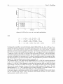
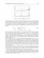
Figure 4.2: Increase of R and J during one operation (Ax = 0.2 [m])
The step size during one movement is limited to Ax = 0.2 [m]. Together with the paper
parameters and equation (4.1) to (4.8), we can quantify the change in reel radii and inertias.
Figure 4.2 shows the percentage of change in inertia over the complete range of reel radii within
one movement. We see that the maximum change in inertia is only 2.5% a t Ri= 20 . lop3
[m]. The change in reel radius is even smaller, hence we will further neglect this non-linear
phenomenon and assume the inertias and reel radii to be constant in each operating point.
This means that locally we take J~= 0 and ~i = 0. Globally equations (4.5) to (4.8) are still
valid.
4.2
Dynamics
Before we can derive the dynamical model, we make a few assumption:
the dynamics of the motor electronics can be ignored
the friction at the reels and capstan can be neglected
0
because of low angular velocities, the friction at servo motors can be modelled using
Coulomb friction only.
the reel radii and inertias may considered to be constant in each operating point
Using Newton's law we can now derive the following set of differential equations:
Part I - Modelling
12
frequency [Hz]
Figure 4.3: F R F of Iml to cp, at
4
reel radii combinations
with
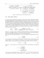
To design the controller, we need the input-output relation from Iml to cpc and Im2 to cp,.
Because the system is symmetric, the transfer functions of both I/O relations are similar, only
opposite in sign (if the capstan rotates in positive direction, reel 1 also rotates in positive
direction, but reel 2 rotates in negative direction). The relation is dependent on the radius of
the reel, so we show the transfer function (figure 4.3) at 4 different reel radii combinations.
A difficulty is that at this stage not all the model parameters are known, so we use estimates.
The motor shaft parameters are provided by the motor supplier. The esimates for the paper
damping and stiffness are obtained from [I]. When a prototype is build, it is possible to identify the parameters to get more accurate values. This identification procedure is described in
chapter 8.1. The parameters used are listed in appendix A.
The systems with R1 = 20 [mm] show an eigenfrequency at f = 250 [Hz], which is introduced
by the motor shaft and coupling. As the radius of reel 1 becomes larger, this eigenfrequency
shifts to f = 100 [Hz]. When designing a controller, this frequency shift can affect the closed
loop stability, so it has to be taken into account. The change in radius of reel 2 has minimum
effect on this transfer function, because of the relative high damping of the paper. Also the
eigenfrequency at f = 1 [Hz], introduced by the paper dynamics, is strongly damped. For
low frequencies we can see a small phase shift due to this eigenfrequency.
In the next chapter a stabilizing controller will be designed. In chapter 6 this model, including the controller and sensors, will be simulated using Matlab Simulink, to check whether
implementation would work in practise.
Chapter 5
Controller design
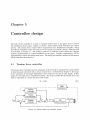
The task of the controller is to keep a constant tension force in the paper and to control
the translation of the paper. Figure 5.1 shows a block scheme which describes the control
system. The tension force control will be implemented as a feedforward controller, which
uses off-line estimation of the reel radii to set the torques on both DC motors. This part will
be described in section 5.1. The position control is a feedback system which uses capstan
position measurements to control translation of the paper. Friction compensation will be
implemented to reduce the steady-state error. The design and stability analysis of this system
will be described in section 5.2.
5.1
Tension force controller
The tension force controller uses the estimation of the reel radii to calculate the torque needed
to keep the paper stretched with a certain tension force. As described in chapter 4, the range
of one operation of the Image Verification Unit is limited to 0.2 [m] in tape length. In this
range the reel radii can be considered constant. The torque needed for the tension force can
then be expressed as a linear function of the radius
I
Friction
Compensation
I-7
I
I
[(PI
Position
Controller
(Pcref
IVU
Motion System .
I
I
Figure 5.1: Block scheme of controller design
(P21
(PC
I
- -I
Part I - Controller design
14
Thus during one operation the required torque can also assumed to be constant. It is then
possible to estimated the reel radii off-line and implement the tension controller as a constant
feedforward signal. The advantage here is that the controller is kept simple. We do not need
an adaptive controller, which would increase the implementation costs. The controller will
also not affect stability.
The value of the required tension force can be obtained from the torque delivered by the slip
couplings at the current system. This torque is set to the value needed at the average reel
radii and is equal to Tt = 3.0 [Nm]. At R,,,
= 30 [mm] this gives Ft = 1.0 . 10-I [N].
Because the capstan has a constant known radius, the reel radii can be estimated from the
measured reel and capstan rotation by
When the rotation can be measured exactly, we only need a very small step to be able to
give an precise estimation of the reel radius. However, because the measurements of all 3
rotation are quantized, we need a larger step to guarantee a certain accuracy of estimation.
We can describe this accuracy as the relative influence of the quantization interval on the
total rotation. This can be expressed as
accuracy =
2nlincrements
- 100
rotation
[%I
If we want to obtain an accuracy of 5% at the rotation of reel 1, we have to rotate cpl =
27r 209
= 0.6 [rad]. The maximum tape translation needed for this rotation is a t maximum
reel radius, hence the required paper displacement x = cplR1,,, = 24 [mm] or cp, = 1.9 [rad].
If we use an encoder with 500 ppr to measure cp,, the accuracy of the measurement will be
- 100 = 0.7
The total accuracy is more than required as will be shown in the
simulations in section 6.3.
[%I.
5.2
Position controller
A requirement for designing the controller is to keep it as simple as possible in order to minimize the implementation costs. Of course, the controller also has to be robust, in this case this
means that it has to be stabilizing for the complete range of reel radii. Other disturbances are
not incorporated here. Because the system with R1 = 40 [mm] the eigenfrequency introduced
by the motor shaft is at the lowest frequency and of the highest amplitude, we expect this
system to have the most critical stability margins. However, if we keep the closed loop bandwidth far below this eigenfrequency, we do not expect any influence of this eigenfrequency on
the stability.
To develop the controller we will approximate the process as single mass for low frequencies
(f < 20 [Hz]). The process transfer function can be written as Hp = ~ ~ 1TOs be~ able
. to
place all the poles and zeros of the closed loop system, we need a PD-controller. With the
controller transfer function Hc = G(rds l ) , we can write the closed loop transfer function
as :
+
where K = GKp. The parameters will now be tuned by choosing frequency domain performance of the closed loop system.
5.2. Position controller
---lo-'
1o"
15
10'
18
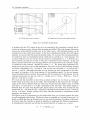
( a ) Closed loop transfer functions
lo'
(b) Nyquist plot of open loop transfer function
Figure 5.2: Controller design plots
A problem with the IVU system is that it is not possible for the controller to inverse the direction by using one motor, because then the paper gets folded. When the change of direction
occurs, the control should be taken over by the other motor. This switching system can be
considered as a piece-wise linear system. If we find a stabilizing controller for both regions
separate, we can say that the system is globally stable. To overcome this switching problem,
it is desired to have an overdamped system, which has no overshoot at a step-response. For
a system without a zero we can say that the system is overdamped as C > 1. However, if a
zero is present and this zero is close to the poles, it introduces extra overshoot. In the real
system, friction introduces extra damping which is not incorporated in the controller design,
so overshoot is then reduced. Therefor we choose C = 1. For closed loop performance demands we do not need to have a high bandwidth. To be sure to stay within stability margins
we choose a bandwidth of wn = 27r [rad/s]. Now we have two real poles at -27r [rad/s] and a
zero at -7r [rad/s]. Although both poles are real, because the zero is dominant t o the poles,
we expect an overshoot in the step response of the simulation model. In the real system,
where Coulomb friction is present, this overshoot will be reduced due to this friction. For the
controller parameters we can now write G = w:/Kp and r d = 2C/w,. With Kp = 31.6 we
have G = 1.25 and r d = 0.32.
If we now use this controller at the system as shown in figure 4.3, we obtain a robust and
stable closed loop system for all reel radii. The bandwidth of the system for the complete
range of reel radii is obtained from the closed loop transfer function, figure 5.2(a), a t 0 [dB]
cross-point. It varies from 1 to 2 [Hz], depending on the reel radii. The phase margin is
obtained from the open loop Nyquist plot, figure 5.2(b), and varies from 75 [deg] for the
system with R1 = 20 [mm] and R2 = 40 [mm] to 88 [deg] for the system with R1 = 40 [mm]
and R2 = 20 [mm]. Further tuning will be done when the controller is implemented at the
prototype, see chapter 8.2.
The friction acts as a disturbance on the steady-state error, so to further reduce this error
we will compensate this friction. The friction force is modelled as Coulomb friction only. To
decide in which direction the friction force acts, we need the direction of rotation of the reels.
In order to keep the controller as simple as possible, we implement the friction compensation
hence
as a feedforward controller and will use the desired direction of rotation
ecTef,
16
Part I - Controller design
Chapter 6
Simulation
Before building and testing a prototype, it is important to know whether it is possible to
implement the concept. This can be verified by making a simulation model which also incorporates the non-linear processes such as the encoders. The model derived in chapter 4 is
implemented in Matlab Simulink. This chapter describes the simulation model and results,
with and without a controller.
6.1
The process Simulink model
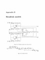
The main model (figure B.l) describes the equations (4.9) to (4.13). We choose the motor
as inputs, because these are the variables that can be controlled. The
currents Imland Im2
angular rotations cpl, cpz and cp, are chosen as outputs, because these are the parameters
that can be measured. To check whether the model behaves as expected, a simulation is
performed.
Figure 6.1 shows a simulation at R1 = R2 = 30 - lop3 [m]. First both motor currents are set
to a positive value, I, = 4.9 .
[A], which is equal to the desired tension force at this
radius. We expect the reels to rotate in positive direction, and due to paper stiffness come
Im.Km.
to a n end deflection of cpi =
,&: = 6.8 - lop2 [rad]. This is shown in figure 6.l(c). By
increasing Im2
for 1 second, we expect the system to accelerate and then maintain a constant
the system will decelerate. This is shown in figure 6.l(d).
velocity. If we then increase Iml,
The tension force, shown in figure 6.l(b), increases during acceleration, but remains at the
desired level during constant velocity.
At the prototype the rotations of both reels are measured by optical sensors which count 209
increments per revolution. These sensors can not detect the direction of rotation. To obtain
a good simulation model, we will extend the main model with a model of these sensors. The
implementation in Simulink is shown in figure B.2. The pulses given by these optical sensors
are counted by a counter, which is shown in figure B.3.
The capstan rotation is measured with a rotational encoder. This device generates A & B
pulses, which can be used for rotation and direction detection. We only have to quantize this
rotation to get the measurement 9,. In simulations we use an encoder with 500 increments
per revolution.
Part I - Simulation
18
(b) Tension force
( a ) Motor currents
08
1
1.2
bme [sl
( c ) Reel rotations f o r t
<2
sec.
( d ) Reel and capstan rotations
F i g u ~ e6.1: Simulation at R1 = R2 = 30 .
[m]
6.2. Reel radii estimation
6.2
19
Reel radii estimation
The reel radii are estimated using the known capstan radius and the reel and capstan rotation,
as described in chapter 5.1, equation (5.2). When implementing this, we must be sure that the
rotation is not reversed, because the optical sensor will only count upwards. The estimation
will then not be accurate. In Simulink this is realized by setting a positive torque at motor
2 to put the system in motion, and we will use motor 1 to keep the paper under tension.
Because the reel radii are not known in advance, we will use the minimum torques required.
The tension torque is thus the torque needed when reel 1 is at minimum radius, the stepping
torque is the torque seeded to overcome the static friction level when reel 2 is at maximum
radius. If the capstan rotation passes the required 1.9 [rad], the system is triggered and the
reel radii are estimated and passed to the controller. The Simulink scheme is presented in
figure B.4.
6.3
Controller implement at ion
To check whether the controller will behave as expected, we have implemented it at the
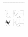
extended Simulink model. The complete scheme is shown in figure B.5. Figure 6.2 shows the
response of the system at R1 = 20 [mm] and Rz = 40 [mm]. We see that the closed loop
behavior is stable and the system is overdamped. The overshoot, which would be introduced
by the zero, is reduced by the Coulomb friction. The tension force is kept at the desired level
during constant velocity. All reel radii combination show the same behavior. From these
simulations we can conclude that it is possible to implement this system configuration, and
obtain good results using a simple controller. A prototype can now be build and tested. The
next chapters describe the implementation and test results of this system.
Part I - Simulation
3n
( a ) Capstan rotation
(6) Reel rotations
(c) Tracking error
( d ) Tension force
Figure 6.2: Closed loop step response
Chapter 7
Practical setup
This chapter describes the test setup of the Image Verification Unit redesign. It consists of
a data acquisition system which can be used from within Matlab and runs in real-time, two
switch-mode drivers to drive the DC motors, two Iron Core DC motors, a quadrature encoder
and two optical sensors.
7.1
Data acquisition system
For testing a system it is important to be able to continually measure and control it. To
do this, we need a data acquisition system which is capable of measuring analog signals
and digital signals (for encoder usage), but can also send out analog or digital controller
signals. To be able to predict and control the timing behavior of a dynamical system, the
data acquisition requires real-time performance. This section describes the implementation of
"soft" real-time measurement and control using the AT-MIO-16-DE data acquisition board
with Matlab Simulink, the Real Time Workshop and Wintarget. An overview of the complete
system is shown in figure 7.1.
1
I
I
I
I
I
- - - Matlab
Simulink
model
Real Time
Workshop
1
I
I
I
!
Wintarget
.
-4
RT executable
IVU
motion system
-
-.
PC &
DAQ-board
L - - - - J
Figure 7.1: Schematic overview of the practical setup
22
Part I - Practical setup
7.1.1 Data Acquisition Card
The AT-MIO-16-DE multifunction 110 board from National Instruments features 12-bit
ADCs with 16 analog inputs, 12-bit DACs with two voltage outputs, 32 lines of TTLcompatible digital I/O, and two 24-bit counter/timers for timing 110.
Analog Inputs
The analog input can be set to measure referenced or non-referenced single inputs and differential inputs in uni- or bipolar mode with a voltage gain varying from 0.5 to 100 [-]. Unipolar
input means that the input voltage range is between 0 and Vref, where Vref is a positive reference voltage of 10 [V]. Bipolar input means that the input voltage range is between -Vref/2
and +Vref/2. At the IVU motion system, the only analog signals that have to be measured
are the optical sensor signals, which are voltages between 0 and 5 [V]. It is also possible to
enable dithering. Dither, or additive white noise, has the effect of forcing quantization noise
to become a zero-mean random variable rather than a deterministic function of the input
signal. When you enable dither, you add approximately 0.5 LSB rms of white Gaussian noise
to the signal t o be converted by the ADC. This addition is useful for applications involving
averaging to increase the resolution of the DAQ board as in spectral analysis. Because for
the sensor measurement we only need to detect low or high logic level, dithering is not enabled. Another board function is multiple-scanning. With multiple-channel scanning you can
increase the scanning speed and sample several signals as nearly simultaneously as possible.
The maximum multiple-channel scanning acquisition rate is identical to the single-channel
acquisition rate for all gains, which is 500 [kS/s]. The settling time of T, = 5 [ps] is not
increased as long as the gain is constant. When scanning among channels at various gains,
the settling times may increase. We will use this multiple-scanning, so the scanning time will
not limit the sampling frequency.
Analog Outputs
The analog outputs can be configured for either unipolar or bipolar output. A unipolar
configuration has a range of 0 to Vref at the analog output. A bipolar configuration has a
range of -Vref to +Vref at the analog output. Vref is an internal reference of +10 [V] or an
external reference between -11 [V] and +11 [V]. The settling time of both output channels is
3 [ps]. The output voltages can not be set simultaneously. In the test setup, we will use both
analog output channels to set the reference voltage of the motor drivers. Because the motors
have to deliver torque in both direction, we shall use the analog output channels in bipolar
mode.
The two 24-bit up/down counter/timers are available for a wide variety of timing and counting applications. Its up/down counting feature is particularly convenient for encoders. When
using quadrature encoders with the DAQ-STC, you have two choices. First, for simple applications, you can connect the encoder directly to the DAQ-STC, without any extra logic or
7.1. Data acquisition system
23
A clock
Encoder
RBlAS
Vss
I
DGND
I
Figure 7.2: Encoder to counter interface using the LS7084
signal conditioning. Although simple to implement, this configuration has the disadvantage
of not being able to discern between stationary vibration of the encoder and real rotation.
Second, you can interface the encoder to the DAQ-STC using a using a quadrature clock
converter IC. This method prevents errors due to jitter and debouncing, and provides higher
measurement resolution. For control purposes we will implement the second method using
the LS7084 quadrature clock converter from LSI Computer Systems. This I C converts the A
and B signals from an encoder into a clock and up/down signal that you can connect directly
to the DAQ-STC. The LS7084 includes lowpass filters to prevent miscounts due t o noise and
jitter. In addition, the LS7804 uses dual one-shots to prevent the miscounting produced by
vibration, or dither. This interface is shown in figure 7.2.
7.1.2
Matlab and real-time
Using the Real-Time toolbox and the lcc-compiler it is possible to compile and run c-code
created from your Simulink model. If this code is generated using the Wintarget template
make file, a real-time executable is made. On execution, Wintarget installs a n interrupt
service routine that executes the code at the right times. The sample rates can vary from 1
[Hz] to what the pc is capable of.
Using this configuration it is also possible to add custom c-code to the Simulink model. In this
way a device driver is created that handles communication between the real-time program
and the DAQ card. In Simulink, this driver is presented as a masked S-function block. The
user can read analog inputs and encoder values from, and write analog outputs to the ATMIO-16DE-10 block. All the card function described in section 7.1.1 can be set by the user.
In appendix D a detailed description of this block is given together with all the files and steps
needed to create a real-time executable.
A problem occurred when trying to compile the generated code, because the DAQ card
requires double and unsigned long variables. If this block code is not generated first, the
variables are not declared at the beginning of a function. In c-code, this results in an error.
This problem can be evaded by making sure that the driver block gets the highest priority.
When the script rtbui1d.m is used for building, all the blocks in the Simulink scheme are set
to priority 1, but the driver block is set to priority -1.
Wintarget shows missed sample hits in an indicator. Real-time performance can be guaranteed
when no samples are missed. Using a PI11 based pc at 400 [Mhz] processor, a sample frequency
of 800 [Hz] can be guaranteed if no other tasks are running. In the measurements we will set
= 0.002 [s].
the sample time to T, =
6
Part I - Practical setup
24
T~~,~~E~~-
r ERROR
- - - - - - - - - r PWM~
AMPLIFIER
M X OR
- FILTER
- - _ I
LCURRENT
- - - SENSING I
Figure 7.3: Block scheme of the L292 motor driver
7.2
DC motor driver
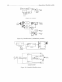
To control the power delivered by the motors, we need a motor driver which linearly transfers
the analog voltage output of the data acquisition board into a current to the motor. We use
the L292 Switch-Mode Driver from SGS-Thomson to perform this task. This is a pulse width
modulation (PWM) type full-bridge driver and is capable of delivering 2 [A] current at 24
[V] with a maximum switching frequency of 30 [kHz]. The L292 consists of a level shifter, an
error amplifier, a current sensing amplifier, a filter and a PWM. A block scheme is presented
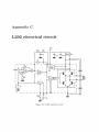
in figure 7.3. The electrical scheme of the motor driver with all its external components is
given in appendix C. The transfer function from the reference input voltage VI to the output
current IM can be written as:
&%
where Gmo =
, Rl, R2, R3 and R4 are internal resistors, VR is the internal reference
voltage, Vs is the supply voltage, LM is the motor inductance and RM is the motor resistance.
All the other variables can be chosen to meet the optimal conditions.
If we look at the DC transfer function ( s = 0), we can calculate the sensing resistance value
from
At the maximum voltage output of the DAQ, VI = 10 [V], the motor current must be at its
maximum value, .IM= 2 [A], hence Rs = 0.24 [a]. In order to be sure that the closed loop
system is stable, we first cancel the pole introduced by the PWM & motor by choosing:
Equation 7.1 is now reduced to a second order system with cutoff frequency and damping
ratio
<
$a,
If we now choose a damping ratio of = we get C = 1.24 lop4RF CF [F]. If we look
at the filter, we see that it has a cutoff frequency of f =
[Hz]. A recommended value
7.3. DC motors
25
frequency [Hz]
Figure 7.4: FRF of the L292 motor driver
for this bandwidth is 3 [kHz], hence RFCF = 5.3 . lop5 [s] and C = 6.6 [nF]. From (7.4) we
now have R = 170 [kR]. If we now choose RF = 510 [R], we obtain CF = 104 [nF]. The Bode
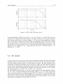
plot of the transfer function is shown in figure 7.4. We can see that the bandwidth is larger
than lo3 [Hz], so the motor driver will not affect the performance of the IVU motion system.
Because the L292 is a PWM motor driver, also the switching frequency must be set. This
has no effect on the closed loop system, but only make the output stage more efficient. The
[HZ]and will be set to 22 [kHz] using Ro = 15
frequency can be expressed as f, =
[kR] and Co = 1.5 [nF].
&
7.3
DC motors
In theory DC motors of any size are able to put the system in motion, but due t o the tension
and friction forces, these motors need to supply a torque from at least the maximum friction
and the maximum tension torque to put the system in motion. We have performed some
experiments to measure the friction torque. We placed a paper roll with maximum diameter
at one reel and measured the current needed to put the reel in motion, thus to overcome the
friction torque. From this measurement, together with the motor constant we can calculate
= 6.1 - lo-' [Nm].
the torque needed: TF = ImKm = 0.1 - 61 For the required tension torque we use the torque applied by the slip couplings, which is
2.5.
[Nm]. The total minimum required torque is then T = 6.4. lo-' [Nm]. The motors
used at the old system have a maximum torque of 2.5.
[Nm], so it is not possible to use
these as direct drive DC motors. For simulation and testing the new concept we use an DC
motor with a continuous torque of 0.45 [Nm], which is more than sufficient. For the motor
specification see appendix E, motor 9904 120 53 707.
Part I - Practical setup
26
7.4
Encoder and sensors
The controller developed in chapter 5 consists of a tension force control loop and a position
control loop. Both controllers use position measurements to calculate the required torques.
For the position control loop we need to measure the position of the paper. It is however
not possible to measure this directly. By measuring the rotation of a capstan with known
diameter, it is possible to get an estimation of the tape translation. To achieve an accurate
estimation, we must be sure that no slip occurs between the paper and the capstan. It is
possible to use the capstan with pressure roll (see figure 2.1) for this purpose. The required
positioning accuracy is 1- low3 [m]. Because the capstan radius is 12.5- 10V3 [E],
the required
[rad]. Therefor we need an encoder
accuracy for the capstan rotation is 1 - 10-~/12.5.
with a minimum of 27r -12.5 = 80 increments per revolution. If, in the future, the print image
is changed, and therefor the accuracy should be increased, it is advisable to use an encoder
more increments than required. For testing and measurements we use an quadrature encoder
with 2500 pulses per revolution. This is a higher resolution than used in simulations, so we
do not expect that it introduces stability problems.
For the tension force control, we need to identify the roll radii. In the current system optical
sensors are present at both reels, which count 209 increments per revolution. The ratio
between capstan rotation and rotation of the reel will give an estimate for its radius, hence
no extra sensors are needed to identify the reel radii.
Chapter 8
Test results
This chapter first describes the verification and identification of the dynamical model. Then
the controller parameters are calculated so optimal performance and stability can be guaranteed. Finally section 8.3 shows results of step responses.
8.1
Parameter identification
In chapter 4 we derived a model to describe the IVU motion system. With the practica~lsetup
we can verify the obtained model, identify the model parameters and tune the controller
parameters described in chapter 5 . This identification procedure will be described in this
chapter.
It is not possible to directly measure the frequency response function of the input motor
current IM to the capstan rotation cp,, because the motor current cannot be directly measured
by the DAQ board. We identify the frequency response function Hpfrom the output voltage u
set in Simulink, and the measured rotation cp,, so it includes the transfer function of both the
DAQ card and the motor driver. In the previous chapter has been shown that the DAQ has
a gain of 0 [dB] with a bandwith much larger than the IVU bandwith, so it has no influence
on the IVU motion system transfer function Hi,,.The motor driver transfer function is also
known, and we can then extract these transfer functions to obtain Hi,,.
The frequency response function is obtained by measuring the sensitivity S. An advantage of
this method is that the system is actuated in closed loop. We will measure the sensitivity by
adding a band limited white noise w to the controller signal u, (see figure 8.1). The sensitivity
can then be obtained from
'Prer
e
PDcontroller
EAQcard
2
DC motor
driver
I" W U motion &
Figure 8.1: Sensitivity measurement
'PC
system
Part I - Test results
28
i'Ef#Ef3
0.9
0 08
1oO
1 0'
1o2
Frequency [Hz]
Figure 8.2: Sensitivity measurement
where Hp is the transfer function of the IVU motion system together with the DC motor
drivers and the DAQ card, thus Hp = (P,(s)/u(s).
To reduce the influence of friction on the frequency response we use a constant velocity
reference. The controller used during the measurement is a PD-controller with P = 1 [V/rad]
and D = 0.1 [Vs/rad]. The system is excited with a random noise with a bandwidth up to
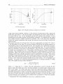
250 [Hz] with a RMS value so u is kept within f5 [V]. The measured S ( s ) is obtained by
averaging 50 time series of 2048 samples at a sample frequency of 500 [Hz] with a Hanning
window and 50% overlap. The measurements are performed at R1 = 38 [mm] and R2 = 22
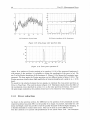
[mm]. Figure 8.2 shows a bode plot of the sensitivity and the coherence of the measurement.
We see that from f = 1 [Hz] the sensitivity S = 0 [dB] which indicates that the closed loop
bandwidth is approximately 1 [Hz].
Now we can extract the controller and the motor driver from this measurement to obtain
the process frequency response function Hi,,. To estimate the parameters, we try to fit the
theoretical transfer function derived in chapter 4 on the measured FRF. Both the phase and
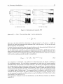
magnitude are considered. Figure 8.3(a) shows both the measured and estimated FRF. We
can see that the measurement data becomes very noisy from f = 60 [Hz], so these frequencies
are not taken into account in the parameter estimation. The system shows a gain increase at
f = 2 [Hz], which indicates mass decoupling of the second (not driven) reel. In the simulation
model this decoupling occurred at f = 1 [Hz]. Hence, the paper stiffness c is higher in the real
system. It also shows a damped eigenfrequency at f = 40 [Hz], which was at f = 100 [Hz]
in the simulation but was less damped. Hence, the motor shaft stiffness c, is lower and the
motor shaft damping k , is higher. Also the process gain shows to be lower, which indicates
larger motor inertia J,. At low frequencies, the phase of the real system turns towards 90
[deg], which means that friction is present in the system. At high frequencies, the measured
FRF shows a larger phase delay than the estimated transfer function. Even at f = 100 [Hz]
the phase still shows a decay. This is introduced by the time delay due to the sampling time
T, = 0.002 [s] and the zero order hold. The time delay in a system causes the original transfer
function Hp to be multiplied by Hd = e-j2TfT. It has constant amplitude IHd(f)l = 1 and
8.1. Parameter identification
(a) Without time delay
29
(b) With time delay
Figure 8.3: Estimated and measured FRF
phase cpd ( f ) = -27r f r. The total time delay r can be expressed as
where T, is the time needed for calculations. In the test setup T, = T,, hence r = 0.003 [s].
Figure 8.3(b) shows the measured and estimated FRF with time delay. We can see that now
also the phase is well estimated.
It is clear that the real system shows the same behavior as the dynamical model derived, and
the P D controller described can also stabilize the real system.
For the feed-forward controller we need an estimation of the friction. Break-away and constant velocity experiments are performed to obtain measurements at different velocities. It is
possible to estimate and compensate the friction using a Stribeck friction model as in equation
(8.3), but the resulting controller would be complicated.
As in chapter 5 is mentioned, it is preferred to undercompensate the friction, resulting in
an overdamped system. For the friction compensation we take then the lowest measured
Coulomb friction which results in a simple controller. The friction is estimated by measuring
the voltage needed to keep the system at constant velocity, averaged over 12 capstan rotations.
At R = 37.5 [mm] this equals 4 complete reel rotations. Figure 8.4 shows the results of friction
measurements and estimation for reel 1. Reel 2 shows the same pattern, but estimation results
in a slightly higher Coulomb part. The measured force in voltages is scaled by the motor
constant and the motor driver DC gain to obtain the friction force in [Nm]. Because only cp,
can be measured accurately, and this rotation is used in feedback, the friction force is show
as a function of @, and not of GI.
The parameters obtained in both the identification and the friction estimation are listed in
appendix A.
Part I - Test results
30
Figure 8.4: Friction measurement and Sribeck estimation
8.2
Controller implementation
Now we have identified all system parameters, we can tune the controller parameters using
the procedure described in chapter 5. We first start with the feedback controller.
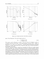
At f = 1 [Hz], the process gain Kp = 25.4. Because the eigenfrequencies introduced by the
motor shaft are more damped, we can probably obtain a higher bandwidth without instability.
Choosing a bandwidth of w, = 47r [rad/s] and damping ( = 1, we obtain G = 6.2 and ~d = 0.16
according to equation 5.4. Figure 8.5 shows the open and close loop responses, the sensitivity
plot for both the measured and the estimated system (including time delay). The nyquist
plot is only shown for the estimated system, because the measured open loop is too noisy at
high frequencies, so the nyquist plot becomes unreadable.
We can see that the closed loop gain at low frequencies is lower in the real system, which is
probably due t o friction. The gain margin obtained is 6 [dB], the phase margin is 70 [deg],
which means that the closed loop system is stable.
For the feedforward controller, we only need to set the friction force depending on the direction
of rotation of the capstan. As shown in the previous section, the friction force shows a very
small dependence on the velocity. Also the friction force has to be undercompensated to obtain
an overdamped system. In the controller we will use the lowest friction force measured, i.e.:
8.3
Closed loop responses
To check wether the system behaves as expected, and is robust and stable for the complete
range of reel radii, experiments are performed.
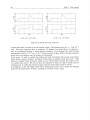
Figure 8.6(a) shows a step response with R1 = 25 [mm] and R2 = 35 [mm]. At t = 0 [s], the
reference steps with -1 [rad]. Motor 2 is now used for position control and motor 1 is used
for tension control. The resulting error is e = 9.77 lop3 [rad]. At t = 3 [s], the reference
steps with +1 [rad]. The direction of rotation reverses, hence motor 1 is now used for position
31
8.3. Closed loop responses
10'
Fiequenoy [HZ
( a ) Closed loop
(b) Sensitivity
(c) Open loop
(d) Nyquist
Figure 8.5: FRF's for measured and estimated system
Part I - Test results
32
1
5
6 05
-0 1
1
2
3
4
5
6
ame [rl
(a) TF = 2.4 . 1oP3 [Nm]
(b) TF = 1 . 5 . lop3 [Nm]
Figure 8.6: Closed loop step responses
control and motor 2 is used to set the tension torque. The resulting error is e = -1.06 .
[rad]. Both step responses show an overshoot. In chapter 5 we stated that it is desired to
have an overdamped system to avoid direction switches. If we decrease the static friction
compensation from 2.4 - 10W3 to 1.5 [Nm], as shown in figure 8.6(b), the step responses
do not have an overshoot and the system is overdamped.
If the motor 1 is used to control the position (in both experiments the second step), figure
8.6(a) shows a larger overshoot and figure 8.6(b) shows a smaller steady state error. This
indicates a higher closed loop gain, which is as we would expect because the radius of reel
1 is smaller than reel 2. We can see that the responses of both reel radii is stable and the
resulting error is within the required margin, thus the closed loop system is robust.
In comparison to the old design, which had a positioning accuracy of *1 [mm], the redesign
improved the performance 10 times, resulting an accuracy of f0.1 [mm].
Chapter 9
Conclusions and recommendations
In this part we have shown that it is possible to obtain good performance and robustness using
simple control strategies and low-cost system parts. The redesign of the Image Verification
Unit uses two DC motors to drive the reels both for positioning and keeping the paper under
tension. This is significantly different from the old system, which uses two DC motors together
with slip couplings to keep the paper under tension, and a stepper motor to position the paper.
Using a PD-controller, feedforward friction compensation and a feedforward tension controller,
the positioning error of the paper in front of the CCD-camera is reduced 10 times in comparison to the present Image Verification Unit. The closed loop system is stable for the complete
range of reel radii, and the position accuracy lies within the camera margin. However, we
have seen that if the reel used for positioning has larger radius, the steady state error is also
larger. This is because the loop gain is smaller at higher radius. Using gain scheduling, where
the controller gain depends on the reel radius, the error can be further reduced. If higher
performance is necessary, a more advanced controller can be developed and implemented.
Now it has been shown that the concept is practicable, the next step is to build a fully functional prototype. Attention must be payed to the implementation of the controller. It might
be possible to implement it digital on the IVU pc, or on a separate micro-controller.
It is also recommended to use other DC motors. The DC motors used have a plastic transmission, and are therefor not highly durable. This transmission also introduces large friction
forces, which increases the steady state error. Brushless DC motors are able to deliver the
same continuous torque using a smaller transmission ratio.
The resolution of the encoder should be chosen according to the desired positioning accuracy.
Simulations have shown that a resolution of 500 increments per revolution is accurate enough.
It is difficult to value the cost reduction, because the cost specification of the old design is
not known at Stork Digital Imaging. We can only say that the costs decrease because the slip
couplings and the stepper motor are eliminated, but increase because a quadrature encoder
has to be used and the electronics (motor driver and controller) must be adjusted. By building
the fully functional prototype more insight is obtained of the specific costs.
34
Part I - Conclusions and recommendations
Part I1
Analysis of the Linear Drive Unit
Chapter 10
Introduction
At the AX-series proofers, problems arise when printing a grey-image. The color spectrum of
this print shows large deviation and a periodic pattern in this error AE. The main disturbance
is a 3 3 9 [mm] pattern, which can be reduced to the performance of the Positioning Unit.
This unit, shown in figure 10.1, consists of a Drum Unit and a Linear Drive Unit (LDU).
The substrate used for printing is positioned on the drum. The task of the Drum Unit is to
maintain a constant rotational speed during printing and to position the drum so the substrate
can be handled. The task of the Linear Drive Unit is to position the print cassettes in front
of the drum. It steps during printing with a step size of 1/12 or 1/24 [mm], depending on the
print resolution. This translation is obtained by rotating a friction wheel (capstan) which is
pressed against a steel strip. The position of the print cassettes is estimated by measuring the
rotation of the capstan. Process disturbances, like variations in the capstan radius, cause the
estimated position to differ from the real position. Here we see a direct relation between the
4 ~ 1 9[mm] patterns in the color spectrum and the LDU, the capstan circumference is namely
18.8 [mm].
In this research first the relation between the position error and the color spectrum error of
the grey image will be analyzed. Chapter 11 describes the origin of measurement errors and
proposes three alternatives to reduce the effect of these errors on the image quality. With
a view to increasing printer productivity, where the speed of positioning must be increased
without loosing accuracy, the performance of the Linear Drive Unit will be analyzed in chapter
12. A few methods to optimize frequency response behavior are proposed.
kwa+uzlrdGuide 8a.4 n p
.
Figure 10.1: Linear Drive Unit
38
Part I1 - Introduction
Chapter 11
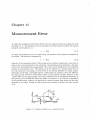
Measurement Error
To realize the translation of the Linear Drive Unit, the capstan is rolls over a guide bar strip
(see figure 11.1). The translation can be expressed as a linear relation between the capstan
radius R, and rotation 8,, i.e.
To obtain the position for use in a control loop, the rotation of the capstan is measured by
an encoder. The position is estimated by
where 13, is the measured rotation. When using such an indirect measurement, care must be
taken to the errors introduced by the estimation. All positioning errors introduce a deviation
in the color, thus influence the image quality. The errors can be classified into two categories,
random and systematic errors. The human eye is not sensitive to a small random error in
the color spectrum of an image, so these errors do not directly influence the image quality.
Systematic errors show a repeatable pattern. If this pattern is constant, it does not influence
the image quality. However, if this pattern shows a (non-constant) periodic behavior, it has
a direct effect on the image quality. The errors introduced due to mechanical inaccuracy in
this system can be divided into these two classes. In section 11.1 we will give a description
of the possible causes. Section 11.2 describes the relation between these errors and the color
spectrum of an image. Finally we will propose some methods to reduce the error (section
11.3).
Figure 11.1: Capstan rotation over a guide bar strip
Part I1 - Measurement Error
40
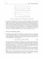
Figure 11.2: Capstan radius deviation and error
11.1
Origin of errors
Varying capstan radius
As we can see from equation (11.2), the position is a linear relation between the capstan radius
and the capstan rotation. Due to production inaccuracy, the real capstan radius R, differs
in all probability from the expected radius R,. The radius can be written as a function of
the rotation, i.e. R, = R,(Qc). Because in the position estimation we use a constant capstan
radius, the error e, = x - 2 introduced by this estimation when the capstan rotates from Q0
to Q1 is
which is thus also a function of the capstan rotation. As for any object, if the capstan rotates
27r [rad], it is in the same position again. Hence, we can write Rc(Qc)
= R C ( 8 , 27r). If
the mean capstan radius R, is equal to the expected capstan radius &, we can see that
over a rotation of 27r [rad], the integral (11.3) is zero. Hence, an error in the capstan radius
introduces a periodic pattern with wavelength
+
This error can thus be classified as a systematic error. At the average expected capstan radius
of R, = 3 [mm], we get A, = 18.85 [rnm].
If the mean capstan radius R, is not equal to the expected capstan radius R,, this will act as
a constant in the integration. The error e, shows also a linear trend.
Now lets say that the capstan is an oval with largest and smallest radii within the specification
of R, = 3 f0.002 [mm], thus behaves as a sine wave over the rotation. The error introduced is
than also a sine with amplitude 0.002 [mm], only shifted $T [rad] due to the integration. This
is illustrated in figure 11.2. The maximum error introduced depends on the initial condition
Rc(Oo).Here it is e, = 4 - 10W3 [mm], which is more than allowed.
11.1. Oriein of errors
41
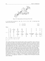
Figure 11.3: Measuring error caused by bearing eccentricity
Capstan bearings
If the capstan has an eccentricity to its bearings, or the bearings are not perfectly aligned, it
causes the capstan to oscillate in the contact point with respect to its center. This can also
be considered as a varying capstan radius, and the error it causes is described in equation
(11.3).
Encoder bearing eccentricity
The encoder is provided with an integral bearing. Under normal circumstances, these bearing
have an eccentricity to the graduation on the encoder disk. This causes a measuring error AOb
as shown in figure 11.3. Due to the eccentricity Ae, the encoder disk center M rotates around
the center of the bearing 0 and translates thus also with regard to the scanning unit A. Only
the translation perpendicular to line A M causes a measurement error. This translation can
be expressed as a cosine of the rotation. Hence, the error is
From this expression we can see that the measurement error AOb has a repeatable pattern
with one full rotation as period. For the encoder used at the AX-series, with mean graduation
radius Rg = 19 [mm], the maximum eccentricity of the bearing AemaX= 5 [pm]. Hence, the
error it causes is at the size of AOb = 3 - 10V4 [rad].
Encoder mounting eccentricity
The encoder is mounted using an externally mounted stator coupling. The purpose of this
coupling is to provide an axial play, yet rotation stiffness, to catch the eccentricity in the
capstan to encoder mounting. Every rotation of the encoder stator is a direct measurement
Part I1 - Measurement Error
42
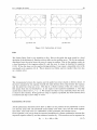
Figure 11.4:Position error due to varying guide bar strip thickness
error AO,. The coupling used is a variant on the Oldham coupling [6]. It has four sharp
folded edges in a thin plate. This provides a good proportion between rotation and axial
stiffness. It is however not completely rotational stiff due to an internal degree of freedom.
In the encoder to capstan mounting there exist an eccentricity due to the unroundness of the
capstan bush. This eccentricity causes the encoder stator to displace axial, but probably also
to rotate. Since the unroundness is repeatable every 27r radians, the obtained measurement
error is a systematic error, and has the same effect on the measurement as the bearing
eccentricity. It is difficult to quantify the size of the error, but even a minor rotation of
AO, = 10W3 [rad] causes a significant error in the position measurement of 3 [pm].
Guide bar strip thickness variation
The capstan is pressed against the guide bar strip to translate its rotation into a translation
of the complete unit (see figure 11.1). The strip is placed against a extrusion profile which
carries the complete unit. The guide bar strip can be seen as a path c(t) = (x(t),y(t)). The
distance travelled by the capstan moving along this path is the integral of speed with respect
to the time travelled, i.e. the path length is
The physical meaning of variable y(t) is the variation in the thickness of the steel strip from
its nominal value, but it also incorporates the flatness of the extrusion profile. If this thickness
is constant, y(t) = 0, we can see from equation (11.6) that the path length is equal to the
position of the printheads, i.e. I = x(t). However, if the thickness is not constant buy depends
on the position x, and thus y(t) = h(x(t)) - ho, we see that the path length is not equal to
the position of the printheads, and the error introduced is el = x - 1.
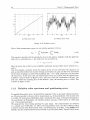
In all probability, the thickness of the steel strip is not constant. It might even be possible that
due to the production process of the strip, the thickness varies at a repeatable wavelength.
This is however not likely and the error on the position can therefor be seen as a random
error.
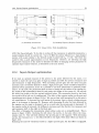
To get an idea of the size of the error the varying thickness causes, figure 11.4 shows a
simulation where y is a function of the position, i.e. y(x) = 0.1 sin(&x) [mm]. We see that
even with this extremely large deviation, the resulting error is very small.
11.1. Origin of errors
43
(b) B e s t case
( a ) W o r s t case
Figure 11.5: Interaction of errors
Dirt
The Linear Drive Unit is very sensitive to dirt. Dirt at the guide bar strip result in a local
deviation of the thickness h, thus has a direct effect on the position error. The dirt is randomly
distributed over the strip, hence the error it causes is random. Dirt at the capstan results in
a local deviation of the capstan radius R,, and the error it causes is described in equation
(11.3). If the dirt stays on the capstan during printing, it can cause a repeatable error with
wavelength as in equation (11.4). This is however not likely, and we consider this error also
as a random error.
Slip
The transmission between the capstan and the guide bar strip is based on friction forces. If
the force actuated by the capstan exceeds the static friction level, slip between the capstan
and the guide bar strip can occur. This slip is a relative motion of the two contact areas,
this means that the real translation x is not equal to the expected translation 2. The slip
causes thus a direct error e, = x - 2. We assume the slip to occur randomly, hence the error
it causes is also random. If the guide bar strip or capstan is polluted, the static friction level
is reduced and slip is more easily to occur.
Interaction of errors
All the phenomena described above have an effect on the position of the printheads. It does
not directly mean that all introduced errors fortify each other, they can also work against
each other. The total error is a combination of the systematic and random errors.
From equation (11.2) we see that the expected translation is a linear combination between the
expected capstan radius R, and the measured rotation 8,. This rotation can be expressed as
em
=
& + A @ bnom
+
(11.7)
Part I1 - Measurement Error
44
(a) With linear trend
(b) Without linear trend
Figure 1I . 6: Position error e
Due to these measurement errors, we can rewrite equation (11.3) as
This equation describes all the systematic errors in the system. Together with the guide bar
strip error el and slip error e,, the total error can be written as
Here the errors due to dirt are not explicitly mentioned, because these can be reduced to e,
and el.
Now lets consider a scenario, where the random errors are zero and where the capstan is an
oval as described before, the encoder bearing eccentricity is 5 [pm] and the error introduced
by the stator coupling is a cosine with amplitude A0, = lov3 [rad]. Equation (11.8) describes
the total error. In the worst case, the measurement errors are in phase and the capstan error
is shifted ./r [rad] as shown in figure ll.s(a). The error e has now a maximum of 6 [pm]. The
best case, where the mounting error is also shifted ./r [rad], the resulting error e is nihil. This
is shown in figure 11.5(b).
11.2
Relation color spectrum and positioning error
To quantify the position error e as described in equation (11.9), we mounted a linear encoder at
an AX-series proofer to obtain a direct measurement x, of the printheads. The encoder used
is a LIDA 477 system from Heidenhain with a resolution of 0.5 [pm]. If mounted according to
the specification of Heidenhain, the absolute position accuracy of this system is f0.05 [pm]
over 1 [m] measuring length.
We measured the error during printing of a grey image. The measurements are obtained
at a sample rate of 500 [Hz]. To reduce the measurement noise, the data is filtered using
a discrete second order Butterworth with a cut-off frequency of 50 [Hz]. Using filtfilt from
Matlab, the data is filtered forward and reversed to get zero phase delay. Figure 11.6(a) shows
11.2. Relation color spectrum and positioning error
45
Figure 11.7: Fourier transform of the error
the measurement error e over 600 [mm]. It shows a large positive linear trend, which indicates
that the capstan radius is larger than expected. Over 600 [mm], the error increased 0.36 [mm]
due to this trend, so the deviation in capstan radius R, - R, = 1.8 [pm]. To highlight the
periodic pattern in the error, we removed the linear trend as shown in figure 11.6(b). The
wavelength of the error with respect to the position can be analyzed using a discrete Fourier
analysis:
with
Xk = inf , x,,
Xe
-
Xe
-
2 ' "" N
.
x
, N = ?Ax
where E is the Fourier transform of the error, Xk the wavelength, N is the number of measurement points, A x is the distance between two measurements and x, is the total measurement
length. For the Discrete Fourier Transform holds E(XNI2+k) = E(XNI2-k), SO the DFT can
be seen as folded around the wavelength XfOld =
Because we use a discrete Fourier
analysis, we must take account for signal-leakage. If there are wavelengths in the signal of
different size than the discrete XI, values, the energy of these wavelengths leaks to the neighbouring wavelengths.
For this analysis, we use N = 1200, thus the shortest wavelength we can see is Xk = 1
[mm]. To reduce the effect of signal-leakage we use a Hanning window. We also take the
error without the linear trend, because this would only introduce more signal-leakage at long
wavelengths. Figure 11.7 shows the amplitude IEl as a function of Xk on two different scales.
We see three high peaks in the amplitude (bottom plot). The first one, at Xk = 18.75 [mm],
is clearly due t o the combination of varying capstan and encoder eccentricities. The second
and the third peaks, at Xk = 150 [mm] and Xk = 300 [mm], are most likely due to the guide
bar strip thickness.
To produce the color grey, all CMYK' colors have to be used, and therefor a grey image is
the most sensitive to system errors. When an image is printed, it is possible to measure its
color spectrum L*a*b values2 dependent on the position. A perfect image will show constant
h he four ink colors used for printing are Cyan, Magenta, Yellow and blacK (CMYK).
his color model is based on the model proposed by the Commission Internationale d'Eclairage (CIE) in
1931 as an international standard for color measurement. In 1976, this model was refined and named CIE
L * a * b. L * a * b color is designed to be device-independent and perceptually uniform. L * a * b color consists
of a luminance ox lightness component (L*) and two chromatic components: the a* component (from green to
red) and the b* component (from blue to yellow).
Part I1 - Measurement Error
46
(b) F o u r i e r transform of the L u m i n a n c e
(a) L u m i n a n c e of grey image
Figure 11.8: Grey-image color spectrum data
10
11
12
13
15
17
20
24
30
40
60
120
inf
A, lrnrnl
Figure 11.9: Cross power spectrum S
values. If we perform a Fourier analysis as in equation (11.10) of the measured luminance L
with respect to the position, it is possible to obtain the wavelength of the error in [m]. We
use I' as the Fourier transform of the luminance L. Figure 11.8(a) shows the Luminance measurement. We show again the Fourier spectrum on two different scales in figure l l.8(b). The
Fourier spectrum clearly shows high amplitudes at long wavelengths and a peak at Xk = 18.75
[mml.
To search for the relation between the two signals, we calculate the cross power spectrum as
S(Xk) = E(Xk)I'(Xk). The result is shown in figure 11.9. This figure clearly shows the effect of
the mechanical errors described in section 11.1 on the color spectrum deviation. To improve
the grey-image consistency, the position errors have to be reduced or even eliminated.
11.3
Error reduction
As shown in the previous section, the difference in real position of the printheads and the
expected position has great effect on the quality of an image. In practise, especially the +I9
[mm] wavelength cause the proofer to fail the quality demands of Stork Digital Imaging. It
is therefor desirable to reduce these errors. This can be done in a few different ways.
The first method is to increase all specifications of the Linear Drive Unit. The maximum
11.3. Error reduction
47
Figure 11.10: Filtered luminance
capstan radius deviation, the encoder mounting eccentricity and the guide bar thickness
deviation (which incorporates the extrusion profile) should all be decreased. This is possible,
however, the system costs would also increase with increasing accuracy. The random position
errors introduced by dirt and slip would still be present in the system. Also due to wear of
the system parts, the errors could increase when using the proofer.
A second method could be to use the spectrum data of a grey (or similar) image to calculate
the expected position error introduced by the Linear Drive Unit. With this data, a correction
of the expected translation (equation (11.2)) with respect to the expected error 6 could be
made, i.e.
However, due to signal leakage of the Fourier transform, the wavelengths can not be determined at 100% certainty. For the wavelengths close to 18 or 19 [mm], we know that these
are most likely introduced by the capstan and encoder errors. The real wavelength is then
approximately as in equation (11.4). If this wavelength could be determined exactly, and the
absolute rotation of the capstan and the shape and phase of the error with respect to this
rotation are known, these errors could be reduced. If these conditions are not known within
a certain margin, correction could lead to larger position error.
To get an absolute measure for the rotation of the capstan, an absolute angular encoder can be
used, so this would not be a problem. The exact X can also be determined rather straightforward, as it is exactly one full rotation of the encoder/capstan. If the luminance data is filtered
using a band pass filter to obtain only the relevant wavelength, also the shape and phase of
the error could be determined. Figure 11.10 shows the luminance filtered with a second orThe result is a relative constant
der butterworth filter with frequency band $ wk
amplitude wave with X z 18.75 [mm], and we could find the relation 6 = f (L,I?, 0,).
With this method, the errors introduced by the varying guide bar thickness, dirt and slip
would still have effect on the image quality. The effect of wear of the capstan and encoder
could be reduced by frequently measure the color spectrum deviation and determine the expected error.
A third method to reduce the position error is to use a direct measurement method. When
measuring the absolute position of the printheads using a linear encoder, the phenomena as
described in section 11.1 have no effect on the position error. The only measurement error
left is the accuracy of the encoder.
This method has more advantages then only providing an accurate measurement. Using the
<
< &.
48
Part I1 - Measurement Error
current indirect measurement, increasing system time performance would be risky, as the
probability slip occurs would also increase. Because slip has no effect on the position measurement using a direct measurement, it is more easy to obtain higher system performance.
Also the requirements of the individual system parts of the Linear Drive Unit can be decreased, while maintaining the same position accuracy.
Currently, during the assembly process at Stork Digital Imaging, it takes much time to optimize the Linear Drive Unit so the proofer meets its quality demands. Also, many service calls
for color deviation in the grey image come in, which cost a lot of money. Often, this color
deviation is only due to dirt or wear of the system. Using the direct measurement method,
both the assembly time and service calls can be reduced. Naturally, all methods described
ask for an investment on one side, and give profits on the other side. It is left for further
research to value all these profits and costs. The decision whether to optimize performance
by changing the Linear Drive Unit, is not based on technical innovation only, but on this cost
analysis.
With a view to increasing printer productivity, where the speed of positioning must be increased without loosing accuracy, the performance of the Linear Drive Unit will be in the
next chapter. A few methods to optimize frequency response behavior are proposed.
Chapter 12
Performance
The performance of a system is defined by all the static and dynamic relations of that system.
Without a model it is mostly difficult to predict how the performance will change when
changing a system parameter. For example, if we want to increase the speed of positioning, it
could be sufficient to use a stronger DC motor. It is however also possible that other factors
are limiting the performance. Sometimes it is possible to derive a model by deduction from
physical laws only, resulting in a white box model. However, if no prior knowledge is available,
a model can be obtained from measurement, resulting in a black box model. The advantage of
the black box approach is that the obtained model incorporates all the phenomena that have
effect on the input-output relation. It is however difficult to reduce this relation to physical
parameters, and it is not always possible to see the effect of a system parameter on the model.
This is possible using the white box model.
To get insight in the physical relations of the Linear Drive Unit, and to be able to predict how
to optimize the performance of the Linear Drive Unit, section 12.1 describes the modelling
of the LDU mechanics using a white box approach. This model is verified by a black box
identification in section 12.3, but first the electronic part of the LDU is described in section
12.2. Section 12.4 describes how to use the system parameters to increase the performance
using the white box model. Section 12.5 describes the effect of the use of friction wheels
as transmission on the performance of the LDU. Section 12.6 describes the identification of
friction in the LDU. Finally, section 12.7 gives an analysis of the controlled used at the LDU,
and how to optimize this.
12.1
Modelling
We define the system boundary as all rotating and translating parts, shown in figure 12.1.
Here the motor, transmission wheel and encoder are modelled as rotating bodies with a
certain inertia. The motor shaft is modelled as a rotational spring/damper with a rotating
body at the end. The inertia of this body is negligible. The capstan is modelled as two
rotational springldampers with a body with a certain inertia in the middle. The complete
unit is modelled as a translating mass, which is connected rigid to the capstan. In this way
we neglect the dynamics of the printheads and other accessories at the LDU. As input we
define the motor current, i.e. u = I,, and as output we define the absolute position x = RcOc
of the mass. The complete system state is defined by four rotations and their derivatives,
Part I1 - Performance
5n
Figure 12.1: Representation of the Linear Drive Unit
i.e. as state vector we choose x = [Om
system can be written as:
Ot
6,
6,
8,
0,
O,]'
. In state space this
Where
1
- b,+Kma
Jm
0
Nk,
Jm
Nb,
Jm
0
1
Nb,
Jt
0
0
0
0
The complete derivation of the dynamical model is shown in appendix I?. Figure 12.2 shows
the input output relation of the system if the damping is neglected. To explain the location
of resonances (pole-pair) and anti-resonances (zero-pair), we can divide the system in three
inertia-spring-inertia subsystems. Of each subsystem we define the actuator as the inertia on
which the input force acts. Such a system introduces a anti-resonance - resonance if the position of the actuator is measured, otherwise it introduces a resonance only. Every resonance
gives a phase shift of -180 [deg], and every anti-resonance gives a phase shift of 180 [deg].
If we consider the capstan spring infinite stiff, the first subsystem is the motor-spring-capstan.
Here the motor is the actuator and the position of the capstan is measured, thus this system
introduces a resonance, at f = 2.1. lo3 [Hz]. The second subsystem is the transmission wheelspring-capstan. Here the transmission wheel is the actuator, and thus this system introduces
also a resonance, here at f = 114 [Hz]. The third system is the capstan-spring-encoder. Now
the position of the actuator, the capstan, is measured, hence this system introduces an antiresonance at f = 254 [Hz] and a resonance at f = 286 [Hz]. After this frequency the phase
delay is 360 [deg].
12.2. Motor Driver
51
:
,-200
3 -400
.!z
a
-500
-600
10'
1o2
Frequency [Hz]
1o3
10"
Figure 12.2: Bode plot
If we choose 8, as output, we would have also seen three resonances, but no anti-resonances.
The phase delay from f = 286 [Hz] is then 540 [deg]. This means that by measuring the position using a rotational encoder, we obtain a different input-output relation than by measuring
the absolute position of the LDU.
12.2
Motor Driver
The motor driver scales the input voltage into a current and controls the current provided
to the motor. The system used here is comparable to the one described in chapter 7, but
uses two separate IC's. The direction or polarity of the output signal depends on a direction
(logic) signal, thus for the reference input holds
0.
Because the torque provided by the motor depends linear on the current (7, = K,I,),
it is
desired that the current is also a linear function of the input voltage. To find this relation,
an experiment is performed.
To measure the current provided to the motor, a resistance of 1 [R] is connected between the
motor and the electronics. The voltage over this resistance is a measure for this current since
V = IR. During the experiment, the motor was fixed to obtain maximum load. Experiments
are performed with both high frequency and static inputs. Up to 2 [kHz], the motor driver
shows the same input-output behavior. For simplicity, here only the measurements with static
input are described.
As input we provided a constant voltage ranging from 0 to 3 [V] with steps of 0.1 [V]. The
measured current is averaged over 7500 samples. Figure 12.3 shows the results. We see that
the relation between the input voltage and the output current is nonlinear. Below V, = 0.8 [V],
[A], which is equal to T, = 8.8 [Nm]. This means that without
the current is 4.2 friction the system starts to move, which is undesired. We see later that the static friction level
is higher than this minimum torque, so this is not a problem. However, if the static friction
level is lower, it could cause instability of the controlled system. For 0.8 5 V, 5 3.0 [V], the
relation could be approximated by a linear relation using the least squares method. Due to a
zener diode, which is used to protect the current controller, input voltages higher than 3 [V]
would result in a maximum current output. The current controller feedback voltage is cut
off at this voltage, so at higher input voltages the error can not be corrected. As a result,
the motor driver delivers maximum output current. In other words, the zener diode causes
instability of the current controller when the input exceeds 3 [V]. The motor is only capable
>
Part I1 - Performance
52
"0
0.5
1
1.5
2
input voltage [V]
2.5
3
Figure 12.3: Motor driver input-output
PD
LDU
Figure 12.4: Experimental setup of Sensitivity measurement
of handling this current for a very short time, so V, > 3 [V] should be avoided. At V, = 3.0
[VJ, the maximum current of 0.23 [A] is thus reached, which corresponds to r, = 4.8 [Nm]. This is less than 40 % of the maximum continuous torque of the motor.
The resulting input-output relation of the motor driver can be divided into three parts, hence
12.3
Identification
We identify the Frequency Response Function (FRF) H L D u ( j w ) by measuring the sensitivity
S in closed loop. The controller used is a PD-controller with H, = 1 . 103(1 0 . 1 ~ obtaining
)~
a open loop bandwidth of 2 [Hz]. A random noise, with a bandwidth of 1000 [Hz], is added
by the Siglab system. The sample frequency of the dSPACE system is set t o 10 [kHz]. The
experimental setup is shown in figure 12.4. To reduce the effects of friction, experiments are
performed at constant velocity. Figure 12.5(a) shows the sensitivity measured at x = 5 [mm
s-'1 and noise RMS value of 0.25 [V]. In this way V, is kept within the linear range of the
motor driver. The FRF is estimated by averaging 50 time series of 8192 samples at a sample
frequency of 2 [kHz]. Different measurements at noise RMS values varying from 0.05 [V] to
0.5 [V] show the same sensitivity. However, if
exceeds 3 [V], HLDUis highly non-linear,
and S is different each experiment.
Figure 12.5(b) shows the resulting LDU frequency response function from 1 t o 250 [Hz]. From
50 t o 220 [Hz] the FRF shows several damped resonances, which can not be directly reduced
to the resonances found in the model. This is probably due to other features mounted at the
+
53
12.4. Input-Output optimization
8
a
O-
Frequency [Hz]
(a) Sensitivity measurement
Frequency [Hz]
(b) Resulting Frequency Response Function
Figure 12.5: Linear Drive Unit identijication
LDU, like the printheads. To be able to reduce all the resonances to physical parameters, a
modal analysis should be carried out. Up to 50 [Hz] the system behaves as a mass-damper
system, with a gain similar to the derived model if scaled with I, = O.lV,. The white box
model is thus a good approximation at low frequencies. However, we will keep the high
frequencies resonances in the model to describe the effect of changing system parameters to
optimize input-output behavior, as described in the next section.
12.4
Input-Output optimization
If we want an optimal response of the system to the power delivered by the motor, it is
desired to make the open loop gain as high as possible and shift the system resonances and
anti-resonances to high frequencies. With increasing process gain also the open loop gain
increases, and it is therefor desired to obtain a high process gain. These conditions depend on
physical system parameters, hence it is possible to use these parameters to optimize performance. At the LDU, the parameters that are free to change are the radius of the capstan R,,
the radius of the transmission wheel Rt and partly the weight of the system M. We will use
the white box model to find the optimal physical values. The resonances found by the black
box model will be left out of consideration. The effect of the capstan radius on the gain and
eigenfrequencies is shown in figure 12.6(a). We can see that with increasing R, on the gain is
not unambiguous. To decrease the total inertia of the system, thus to obtain a higher process
gain, it is necessary to decrease R,. However, with decreasing R, also the force delivered by
the capstan on the mass is decreased, and as a result also the process gain is decreased. If
the capstan radius is increased, the stiffness kc increases and thus the first two resonance and
anti-resonance shift to the right in the Bode plot.
The effect of changing the transmission wheel radius is also not so straightforward. This is
shown is figure 12.6(b). Reducing Rt will reduce the inertia Jt, but also reduce the transmission ratio N. This will both influence the process gain in the opposite. With decreasing
inertia, the resonance at f = 114 [Hz] will shift to the right. Both these effects are shown in
figure 12.6.
Reducing the mass M will always result in a higher process gain, but this effect is negligible.
Part I1 - Performance
54
4 0
- Rc=3 [mm]
-140-160-180
1 0'
1o2
Frequency [Hz]
1 o3
(a) varying Rc, Rt = 30 [mm]
(b) varying Rt, Rc = 3 [mm]
Figure 12.6: Eflect of varying system parameters on input-output relation
The first two resonances will shift to the right when reducing the mass.
To obtain the optimal gain for this LDU model, the capstan radius should be increased to
R, = 6.2 . i ~ [m]
- and
~ the transmission wheel radius should be decreased to Rt = 23 . 10W3
[m]. The increase of the process gain at low frequencies is 4 [dB].
This optimization gives a first good approximation, however to find the optimal physical
values at the real system black box identification measurements with different capstan and
transmission reel radii should be carried out.
12.5
Friction wheel transmissions
The use of friction wheels (motor shaft, transmission wheel and capstan) put a large limitation
on the maximum allowable motor torque. The contact force in these friction wheels is inversely
proportional to the radii of these wheels. If this force exceeds the static friction level in these
contacts, slip will occur. The static friction can be expressed as a linear relation between the
normal force and a friction coefficient f , i.e. F, = fFN [N]. For dry steel contacts f = 0.8,
but due to dirt the value o f f can significantly decrease, and slip is more easily to occur. The
motor is pressed against the transmission wheel with a normal force of FN = 12 [N], hence
= 14 [mNm], which is
the maximal torque the motor can deliver before slip occurs is T,
more than the maximum continuous torque the motor is capable of. The capstan is pressed
against the guide bar strip with a normal force of FN = 20 [N], thus the maximum torque the
= 2.5 [mNm]. It is then desired to
motor can deliver before the capstan starts to slip is T,
increase the wheel radii or to increase the normal force.
The most significant limitation on the performance is thus the transmission between the
capstan and the guide bar strip. To optimize this, the first step is to increase the normal
force to its maximal value, i.e. the value where no plastic deformation the guide bar strip, the
capstan or the bearings occurs. If this should be no limitation, we can say that FN 2
where rm is the maximum torque the motor is capable of. For the present design this means
that FN 2 125 [N]. For the optimized system as described in section 12.4, the pressure force
can be reduced to FN 1 4 6 [N].
12.6. Friction
55
Figure 12.7: Linear Drive Unit controller
12.6
Friction
Friction is a combination of various phenomena, which all depend on the relative displacement and velocities between two surfaces. Normally, the friction is described by the Stribeck
effect. This means that the friction force may decrease continually from the static friction
level and increase with increasing velocity (equation (8.3)). However, near zero velocity and
for small displacements the friction shows a nonlinear behavior, called stiction. Physically
this phenomenon can be interpreted as two moving surfaces that are in contact by a large
number of bristles with a certain stiffness. As a result, the system acts as a spring in this
region. In high precision systems, this effect could cause significant limitation on the position
accuracy.
In the Linear Drive Unit, the presliding behavior could be caused by the linear carriage. If
the stiction phenomena is present, the frequency response function measured with excitation
below the static friction level should result in a spring-mass system [7]. Experiments show
that the Linear Drive Unit behaves as a normal mass system with small damping. This does
not directly mean that the system does not show this behavior, but we can conclude that the
sticking regime smaller than the encoder resolution. Since the static friction level depends
on the normal force between two surfaces, the presliding regime is likely t o increase with
increasing weight of the Linear Drive Unit. This effect should thus be taken into account
when changing the construction weight, for example at the Eagle 4 series.
To quantize the Stribeck effect, break-away and continuous velocity experiments are performed. The break-away experiments show a static friction level of F, = 0.93 [V] for positive
direction and F, = 0.88 [V] for negative direction. This difference is probably caused by the
flexible cable support, which acts as a very weak spring on the LDU. The constant velocity
experiments do not show a decrease in friction force for small velocities, nor a significant
viscous friction level. This can also be seen from the identified transfer function in figure
12.5(b). Viscous friction causes the slope of the transfer function to be -1 (or -90 [deg] phase
delay) at low frequencies, which is not the case.
12.7
Controller
The task of the controller is to track a fixed reference path, resulting in a minimum positioning
error. The first requirement to achieve this, is to obtain a stable closed loop system, i.e. all
the poles of the closed loop transfer function must be placed in the left half plane. Because
there are uncertainties in the Linear Drive Unit, such as varying capstan radius, we must
make sure that the closed loop system is robust stable. To reduce the sensitivity of the plant
to deviations in the process and input and output disturbances, it is desired to have a high
open loop gain in the frequency band of interest. For fast tracking, it is desired to obtain
Part I1 - Performance
56
1o"
(a) Closed loop system
10'
Frequency [Hz]
(b) Sensitivity
Figure 12.8: Transfer functions with present controller
a high closed loop bandwidth. However, in the presence of measurement noise, making the
closed loop gain close to 1 also has the effect of transmitting the sensor noise directly to
the output and the error. So the bandwidth should not be greater than necessary to meet
specifications on set-point response and disturbance reduction. It is desired that the closed
loop transfer function is rolled off outside the passband. Also, if the closed loop bandwidth
exceeds the natural bandwidth of the process, the actuator may not be able to provide the
required power.
The present controller of the Linear Drive Unit can be represented as in figure 12.7. Here is
w the disturbance on the input, the process deviation like friction and varying capstan are
represented by d and v is the measurement noise. The controller can be divided into two parts,
a velocity feedback loop (inner loop), and a position feedback loop. The velocity feedback
adds extra damping to the system at all frequencies. This will result in a slower system and
is therefor not recommended to use.' The position controller used is a Proportional-Integral
controller. This controller does not provide higher gain at high frequencies to increase the
bandwidth. Figure 12.8 shows the closed loop frequency response and the sensitivity of the
resulting system with controller parameters used as implemented in practice. The system
bandwidth is approximately 8 [Hz]. The obtained gain margin is only 2 [dB], which is very
small. With only small process deviations, the closed loop system could become unstable.
To find a more robust and optimal controller H, for this system, a lot of techniques are
available. In practise the Proportional-Integral-Derivative or lead-lag controller is widely
used. The transfer function of this controller is
where a < 1 (lag) and ,6 > 1 (lead). The lag compensation is used to increase the DC
gain to reduce the steady state error. The time constant TI is chosen large to obtain a pole
close to the origin. a is chosen such that it leaves the closed loop system undisturbed in
the neig!borhood of the cross-over frequency, where the most critical stability margins are.
The lead compensation is used to increase the bandwidth of the closed loop system. 70 and
beta must be chosen such that the desired bandwidth is reached. To reduce the effect of the
process resonances, the controller can be extended with a notch filter to reduce the controller
'Compensation with a velocity feedforward would result in a Differential controller.
12.7. Controller
57
Frequency [Hz]
10'
Frequency [Hz]
(a) Controller
(b) Open loop
(c) Closed loop
(d) Sensitivity
10'
I 0'
1o3
Figure 12.9: Transfer functions with lead-lag controller
gain at these frequencies. The notch transfer function is
This creates a notch at frequency w, [radls]. The ratio between the damping CZ and Cp is
o+r at
a measure of the size of the notch. At the notch frequency, the gain is IH,I = &,
frequencies w << wn and w >> w,, the gain is 1. The gain reduction introduced at the notch
To obtain a high roll-off rate at frequencies larger that the desired bandwidth, a
is thus
low-pass filter can be used.
With these controller and filters, a closed loop bandwidth of 50 [Hz] can be easily obtained
at the Linear Drive Unit. Figure 12.9(a) shows a bode plot of a lead-lag controller with two
notches and a 2nd order low pass filter. The resulting closed loop system (controller applied to
the measured plant FRF) is shown in figure l2.9(c). The obtained bandwidth is 52 [Hz], with a
gain margin of 11 [dB] and a phase margin of 60 [deg]. We see that the system is less sensitive
to disturbances and process variations. To further optimize the performance, in addition to
feedback a feedforward controller Hffw can be used. The torque to be delivered by the motor
can be computed by using the inverse of the process transfer function. Often an approximation
$.
Part I1 - Performance
58
Figure 12.10: Optimized LD U controller
of HLDUis used to simplify this computed torque controller. Also disturbances like friction
can be taken into account using feedforward compensation. A feedforward controller does not
affect the stability of the closed loop system. The optimized control scheme is presented in
figure 12.10.
Chapter 13
Conclusions and recommendat ions
The analysis of the Linear Drive Unit has shown that the indirect measurement of the printhead position used, has direct effect on the image quality. The color spectrum of a grey-image
shows significant correlation with the spectrum of the measurement error. This measurement
error is introduced by the LDU mechanics. The capstan radius, the encoder mounting eccentricity and the encoder bearing eccentricity introduce h18.8 [mm] patterns, which is the
circumference of the capstan. The guide bar strip can also introduce periodic patterns. At
the research machine these wavelengths were 150 and 300 [mm]. Dirt at the system has a
similar effect on the measurement error as a deviation of the capstan assembly or guide bar.
All slip in the system causes a direct measurement error, and therefor affects the image quality. It does however not directly mean that a deviation in the mechanics introduce a direct
measurement error. Because of the interaction of these errors, these can amplify or weaken
each other.
The error can be eliminated in various ways. One way is to increase all mechanical requirements, like the roundness of the capstan. This is however very costly and probably not
practical realizable. A second method is to use the color spectrum measurement to calculate
the expected positioning error and correct the measurement for this. This is however only
possible for the patterns introduced by the capstan assembly, because only this wavelength is
known within certain margins. A disadvantage of this method is that the effect of dirt, slip
and varying guide bar thickness would still have effect on the image quality. The third, and
most obvious method, is to directly measure the absolute position of the printheads using a
linear encoder. The only measurement error left is the accuracy of the encoder, and thus all
phenomenon described have no effect on the image quality.
The choice of whether to optimize the measurement is based on investment costs and profits,
and is left for further research at Stork Digital Imaging.
The identified input-output relation between the Linear Drive Unit input
and output x
shows several damped resonances, which can not be directly reduced to the (anti-)resonances
found in the white box model. Up to 50 [Hz], the white box model gives a good approximation
of the LDU and can be used for analysis. Optimization of the input-output relation shows
that, theoretically, the highest process gain is obtained when the capstan radius is increased
to R, = 6.2 [mm] and the transmission wheel radius is decreased to Rt = 23 [mm]. Identification measurements with different capstan and transmission reel radii should find the practical
optimal values.
The use of friction wheels put a large limitation on the performance of the LDU, as the
60
Part I1 - Conclusions and recommendations
maximum allowable motor torque is decreased significantly. Now, slip occurs when the motor
delivers a torque larger than 2.5 [mNm]. The pressure force of the capstan against the guide
bar strip should be increased to 125 [N] to eliminate slip.
At the LDU the friction can be modelled by Coulomb friction only. It does not show a signification viscous friction level, nor stiction for small displacement near zero velocity. Because
friction acts as a disturbance on the process, and increases the steady state error, it must
be taken into account. With increasing weight of the LDU, the stiction regime is likely to
increase, and when redesigning the system also this phenomenon can significantly limit the
performance.
The present controller can be divided into two parts. The first part is a velocity feedback,
which only adds extra damping to the system. This results in a slower system and is therefor
not recommended to use. The position controller used is a Proportional-Integral controller,
which provide high gain at low frequencies to decrease the steady state error, but not at
high frequencies to increase the bandwidth. The closed loop system is close to instability.
With a lead-lag controller with notches at the resonance frequencies and a low-pass filter to
reduce high frequent measurement noise, a more robust closed loop system can be obtained
with a higher bandwidth and smaller sensitivity. Using a computed torque controller and
feedforward friction compensation can further optimize the performance.
References
[I] R.A.Benschop
Fast Access in Tape Drive Systems.
Natlab Technical Note Nr. 255195, Eindhoven (1995)
[2] The Mathworks, Inc.
Real T i m e Workshop.
Natick, Massachusetts, USA, (1999)
[3] The Mathworks, Inc.
Target Language Compiler Reference Guide.
Natick, Massachusetts, USA, (1999)
[4] National Instruments.
A T - M I 0 E Series User Manual.
Austin, Texas, USA, (1994)
(51 National Instruments.
Ni-Daq Function Reference Manual for P C compatibles.
Austin, Texas, USA (1999)
[6] Precision Engineering.
Constructiepricipes 1.
TUE, Eindhoven (1997)
[7] R.H.A. Hensen, M.J.G. v.d. Molengraft and M. Steinbuch
Frequency domain identification of dunamic friction model parameters.
To appear in IEEE Transactions on Control Systems Technology.
[8] P.R.Bhlanger.
Control Engineering: A Modern Approach.
Saunders College Publishing, Orlando, Florida, USA (1995)
62
REFERENCES
Appendix A
Parameter values
This table shows the parameters used in simulation and identified as described in chapter 8.1.
For the parameters which depend on the reel radii, we use R1 = 40 [mm] and R2 = 20 [mm].
simulation
identified
4.5e2
1.2el
1.25el
1.3e-2
1.5e-3
1.9e-4
8.2e-6
1.0e-6
5.0e-6
1.7e3
3.7e-2
0.5e-3
2.0e-2
0.2e-3
6.le-2
3.8e-2
2.2e-2
2.0e-2
1.25e-3
0.002
2.4e-3
description
spring constant paper
torsion spring constant motor shaft
damping constant paper
torsion damping constant motor shaft
Inertia DC motor
Inertia reel & paper roll 1
Inertia reel & paper roll 2
Inertia reel & paper roll 2
Inertia capstan
mass density paper
tape height
tape thickness
reel mass
reel mass
Motor constant 1
radius paper roll 1
radius paper roll 2
minimum radius paper rolls
radius capstan
sample time
Friction force
64
Amendices - Parameter values
Appendix B
Simulink models
462
42
Tck2
44
464
4
t
Damper
& spmg4
-
Figure B.1: Simulink model of the main process
Figure B.2: Optical Sensor
Appendices - Sirnulink models
66
Source
Figure B.3:Counter
Tspan
Figure B.4: Sirnulink model of initialization procedure
-+[qlq2qc]
[RlhR2-F[Rl"R2"l
--+phi-c-ref
in~tializatton
[Irnl lm21
+lrnl
+
92
+lrn2
3sc
ql
Controller
qc
extended model
Sine W a v e
Subsystem 'Controller'
Figure B.5:Controller Sirnulink scheme
-
Appendix C
L292 electrical circuit
Figure C.l: L292 electrical circuit
68
Appendices - L292 electrical circuit
Appendix D
Data Acquisition
In this appendix a detailed description is given of all the files and steps needed to generate
and run the real-time code. We first start with an overview of all files.
ATMIO16DE.c
ATMIO16DE.dll
ATMIOl6DE.mdl
ATMIO16DE.tlc
NIDAQ .h
N1DAQCNS.h
NIDAQ32.lib
NIDEX32.lib
RTSETUP .m
RTBUILD .m
RTSTART .m
S-function driver used to communicate with the Simulink driver block
mex file of ATMI 0l6DE.c
Simulink model with driver block
inlined S-function driver used in code generation
Nidaq header file
Nidaq header file
Nidaq library file
Nidaq library file
m-script used for setting all model parameters
m-script which starts the building process
m-script used to start the real-time executable
These files all have to be installed in the MATLAB-ROOT\NIDAQ directory and must be added
to the Matlab path. To use these files, Nidaq 6.9 and Wintarget 2.0 must be installed on
the system, together with Matlab r12, Real-Time Workshop and the Matlab LCC-compiler
from the Mathworks. An other compiler may also be used, but then the libraries have to
be converted. With Wintarget w t -1cc .tmf is supplied. This is the target make file used in
code generation. To run properly, $ (MATLAB-ROOT)\nidaq\nidaq32.lib must be added to
the S-function libraries S-FUNCTIONS-LIB in this file. For Visual C users, the file w t - v c .t m f
must be changed accordingly.
We will now give a full description of all files summarized above, except for the Nidaq files,
and start with the Driver block.
Simulink Driver block
The driver block is a masked S-function. It calls ATMIOl6DE .dl1 upon opening and closing.
The parameters needed for setting up the DAQ board can be entered in the parameter list,
these are described below.
70
Appendices - Data Acquisition
( a ) Szmulink block
(b) block parameters
Figure D.l: Simulink driver block
This number should correspond with the Nidaq device number.
An ascending vector of Encoder channels to be scanned.
Set to -1 if no encoder channels have to be used.
Analog Input Channels An ascending vector of Analog Input channels to be scanned.
Set to -1 if no analog inputs have to be used.
Hardware Gain
Vector of hardware gains corresponding to analog input vector.
If a gain of 0.5 is to be used, the value must be set to -1.
Vector of input modes corresponding to analog input vector.
Input Mode
0 = Differential, 1 = RSE, 2 = NRSE
Vector of polarities corresponding to analog input vector.
Polarity
0 = Bipolar, 1 = Unipolar
Scalar value that disables (0) or enables (1) dithering.
Dithering
Dithering can not be set per channel.
Analog Output Channels An ascending vector of Analog Output channels to be set.
Set to -1 if no analog output channels have to be used.
Device Number Code
Encoder Channels
ATMIO16DE.c
This c-code file is an S-function to be used with the driver block. It gets all parameters entered
in the block, checks the111 for some conditions and passes these values to the inlined S-function
upon program building. It also sets the number of output and input ports according to the
number of channels to be used. The encoder channels are mapped to the first ports. When
running simulation, it sinks the analog output and generates analog and encoder inputs, all
zera-valued. Further examination is left to the reader, and we will only refer to the Real Time
Workshop User's Guide [2]. Below the full code is presented.
Data Acauisition
71
#ifndef MATLAB-MEX-FILE
#error "Fatal Error: ATMIO16DE.c can only be used to create C-MEX S-Function"
NUM-S-FUNCTION-PARAMS
DEVICE-NUMBER-PARAM
ENCCHANS-PARAM
AICHANS-PARAM
GAIN-PARAM
INPUTMODE-PARAM
POLARITY-PARAM
DITHER-PARAM
AOCHANS-PARAM
SAMPLE-TIME-PARAM
DEVICE-NUMBER
ENCCHANS
AICHANS
GAIN
INPUTMODE
POLARITY
DITHER
AOCHANS
SAMPLE-TIME
((real-T) (mxGetPr(DEV1CE-NUMBER-PARAM)[O]))
(mxGetPr (ENCCHANS-PARAM) )
(mxGetPr(A1CHANS-PARAM))
(mxGetPr(GA1N-PARAM))
(rnxGetPr (INPUTMODE-PARAM))
(rnxGet~r(~oLAR1TY-PARAM))
( (real-T)
mxGetPr (DITHER-PARAM) [O] )
(mxGetPr(A0CHANS-PARAM))
((real-T) (mxGetPr(SAMPLE-TIME-PARAM) [O]))
#define MDL-CHECK-PARAMETERS
static void mdlCheckParameters(SimStruct *S)
static char-T errMsgC2561;
boolean-T allParamsOK = 1;
if (mxGetNumberOfElements(SAMPLE-TIME-PARAM) ! = 1) (
sprintf (errMsg, "Sample Time must be a positive scalar.\n") ;
allParamsOK = 0;
goto EXIT-POINT;
3
if (mxGetNumberOfElements(A1CHANS-PARAM) == 0) (
sprintf(errMsg, "If no analog inputs should be used enter -1.");
allParamsOK = 0;
goto EXIT-POINT;
3
if (mxGetNumberOfElements(ENCCHANS-PARAM) == 0) (
sprintf(errMsg, "If no encoders should be used enter -1.");
allFaramsOK = 0;
goto EXIT-POINT;
3
if (mxGetNumberOfElements(A0CHANS-PARAM) == 0) (
sprintf(errMsg, "If no analog ouputs should be used enter -1.");
Appendices - Data Acquisition
72
allParamsOK = 0;
goto EXIT-POINT;
I
if (AICHANS[O] <O)
return;
else(
if (mxGetNumberOfElements(GA1N-PARAM) != NUM-AI) (
sprintf (errMsg , "Hardware Gain must have %i parameters.\nu',
NUM-AI) ;
allParamsOK = 0;
goto EXIT-POINT;
I
if (mxGetNumberOfElements (INPUTMODE-PARAM) != NUM-AI) (
sprintf(errMsg, "Hardware Gain must have %i parameters.\n",NUM-AI);
allParamsOK = 0;
goto EXIT-POINT;
3
if (mxGetNumberOfElements (POLARITY-PARAM) != NUM-A1 ) (
sprintf(errMsg, "Hardware Gain must have %i parameters.\nol,NUM-AI);
allParamsOK = 0;
goto EXIT-POINT;
I
if (mxGetNumberOfElements(D1THER-PARAM) != I) (
sprintf(errMsg, "Hardware Gain must have 1 parameters.\nU);
allParamsOK = 0;
goto EXIT-POINT;
1
I
if (AOCHANS[OI <O)(
if (mxGetNumberOfElements (AOCHANS-PARAM) > 1) (
sprintf(errMsg, "Analog output channels must be either 0, 1 or [O I].
If no analog output should be used enter -1.\nW);
allParamsOK = 0;
goto EXIT-POINT;
1
I
if (ENCCHANS COI (0)(
if (mxGetNumberOfElements (ENCCHANS-PARAM) > I) (
sprintf(errMsg, "Encoder channels must be either 0, 1 or [O 11.
If no encoder should be used enter -I.\nu);
allParamsOK = 0;
goto EXIT-POINT;
I
3
EXIT-POINT:
if ( ! allParamsOK ) (
ssSetErrorStatus(S , errMsg) ;
I
1
static void mdl~nitializeSizes(SimStruct *S)
C
ssSetNumSFcnParams(S , NUM-S-FUNCTION-PARAMS) ;
#if defined(~ATLAB-MEX-FILE)
if ( ss~etNumSFcn~arams
(S) == ssGetSFcnParamsCount(S)
mdlcheckparameters(S) ;
if ( ss~etErrorStatus(S) ! = NULL ) (
return;
) (
Data Acauisition
3
3 else
(
return;
3
#endif
int-T i;
for (i=O; i < NUM-S-FUNCTION-PARAMS; i++) (
ssSetSFcnParamNotTunable(S , i) ;
3
3
if (AOCHANS 101 <O)<
if ( !ssSetNumInputPorts(S, 0) ) return;
1
if (AOCHANS[O] >=O)(
if ( !ssSetNumInputPorts(S, NUM-AO) ) return;
3
€
int-T iPort ;
for (iPort = 0; iPort < ss~et~umInputPorts(S);iPort++) (
ss~et~nputPort~idth(S,
iPort, I);
3
3
if (AICHANS [O] <C && ENCCHANS LO] (0)i
if ( !ss~et~umOutputPorts(S,
0) ) return;
3
if (AICHANS[O] <O && ENCCHANS[o] >=O)(
if ( !ss~et~umOut~ut~orts(S,
NUM-ENC) ) return;
1
if (AICHANS LO] >=0 && ENCCHANS [O] (0)(
if ( !ssSetNumOutputPorts(S, NUM-AI) ) return;
3
if (AICHANS[0] >=0 && ENCCHANS [O] >=O)C
if ( !ssSet~umOutputPorts(S, NUM-A1 + NUM-ENC) ) return;
3
int-T oPort;
oPort++) (
for (oPort = 0 ; oPort < ss~et~umOut~ut~orts(S);
ssSetOutputPortWidth(S, oPort , I) ;
3
3
ssSetNumSampleTimes( S, I) ;
3
static void mdl~nitializeSampleTimes(SimStruct *S)
ssSetSampleTime(S , 0, SAMPLE-TIME) ;
ssSetOffsetTime(S, 0, 0.0) ;
3
#define MDL-START
static void mdlStart (SimStruct *S)
if (ssGetSimMode(S) == SS-SIMMODE-NORMAL) C
mexPrintf("\n The outputs of the DAQ-board block '%s' will be set "
"to zero during simulation in Simulink.\nl',ssGetPath(S));
3
73
Appendices - Data Acquisition
74
static void mdl0utputs(SimStruct *S, int-T tid)
C
int oPort;
for (oPort = 0; oPort < ssGetNumOutputPorts(S); oPort++) (
real-T *y = ssGetOutputPortRealSignal(S, oPort);
yC0l = 0.0;
3
3
static void mdlTerminate(SimStruct *S)
C
1
#define MDL-RTW
static void mdlRTW(SimStruct *S)
C
if
( !ss~riteRTWParamSettings(S,8,
)
SSWRITE-VALUE-VECT,
SSWRITE-VALUE-VECT,
SSWRITE-VALUE-VECT,
SSWRITE-VALUE-VECT,
SSWRITE-VALUE-VECT,
SSWRITE-VALUE-VECT,
SSWRITE-VALUE-NUM,
SSWRITE-VALUE-NUM,
1(
"EncChans", ENCCHANS, NUM-ENC,
AOChans" , AOCHANS, NUM-A0 ,
"AIChansN,AICHANS, NUM-AI,
"Gain", GAIN, NUM-A1 ,
"InputMode", INPUTMODE, NUM-AI,
"Polarity", POLARITY, NUM-AI,
"DeviceNumber", DEVICE-NUMBER,
"Dither1',DITHER
return;
3
3
#ifdef MATLAB-MEX-FILE
#include "simulink.c"
#.else
#include "cg-sfun.hW
#endif
This inlined c-code file describes three function S t a r t , Outputs and Terminate. We use
function from the Nidaq libraries. These function are namely highly optimized for timing and
speed of execution.
S t a r t , performed when starting the real-time executable, but prior to starting the execution
time, initializes the DAQ card, sets the dithering, initializes the analog inputs to the parameters set in the driver block, sets the analog output to the internal bipolar 10 [V] reference
and immediate update, and finally sets the counters to event-counting. The initial count is
set to half the counter size, to avoid initial counter jumps (if the counter goes through zero
downwards, or through 224 upwards, the count jumps 224 counts).
In Outputs the communication with the DAQ card is described. To increase execution speed
and efficiency, care is taken to reduce the use of variables. First the encoders are read, then
the analog inputs are scanned and finally the voltages are written to the analog outputs.
Data Acquisition
75
In Terminate the encoders are reset to zero and the analog output voltages are set to 0 [V].
Further examination of the code is left to the reader, and we will only refer to the Target
Language Compiler Reference Guide [3]. Below the full code is presented.
%function BlockTypeSetup(block, system) void
%if !EXISTS(rlINCLuDE-NIDAq-H1l)
%assign ::INCLUDE-NIDAQ-H = I
%openfile buffer
/ * Include information about the 1/0 board * /
#include f1c:\matlabr12\nidaq\nidaq.h"
%closefile buffer
%<LibCacheIncludes(buffer)>
%endif
%if !EXISTS("INCLUDE-NIDAQCNSSH1l)
%assign ::INCLUDE-NIDAQCNS-H = 1
%openfile buffer
/ * Include information about the 1/0 board */
#include "c:\matlabrl2\nidaq\nidaqcns.h"
%closefile buffer
%<LibCacheIncludes(buffer)>
%endif
%endfunction %% BlockTypeSetup
%function Start(block, system) Output
%assign
%assign
%assign
%assign
%assign
%assign
%assign
aiChans
gain
dither
inputMode
polarity
numAI
chIdx = 0
= SFcnParamSettings.AIChans
SFcnParamSettings.Gain
SFcnParamSettings-Dither
= SFcnParamSettings.InputMode
= SFcnParamSettings.Po1arity
= SIZE(aiChans,l)
=
=
short deviceNumberCode;
short AIChanVect [%<numAI>l;
short GainVect [%<numAI>] ;
%% Initializing the DAq board
Init-DA-Brds(1, &deviceNumberCode);
%%deviceNumberCode should be 37
%%Dithering on/off
MIO-Conf ig(1, %<CAST("Number", dither) > $0);
0 0
LLConfiguring the analog input ports
%foreach oPort = numAI
AiChanVect :%<oPort>] = %<CAST("Numberfr,ziChans[oPort] ) > ;
GainVect [%<oPort>] = %<CAST ("Number",gain [oPort] ) > ;
AI-Conf igure(1,%<CAST("Number",aiChans[oPort] ) > ,%<CAST("Number",
inputMode [oPort] ) > $0,%<CAST(I1Number" ,polarityCoPort] ) > ,0);
%endf oreach
Appendices - Data Acquisition
76
%%Configuring both the analog output ports:
%%Bipolar, Internal reference 10V and Update when written to
AO~Configure(l,O,O,O,10,0);
AO~Configure(l,l,O,O,10,0);
%%Configuring the counters for use with an encoder
GPCTR-CO~~~O~(I,ND-COUNTER-O,ND~RESET);
GPCTR-Control(1 ,ND-COUNTER-1,ND-RESET) ;
GPCTR-S~~-A~~~~C~~~O~(~,ND-COUNTER-O;ND-SIMPLE-EVENT-CNT);
GPCTR-S~~-A~~~~~~~~O~(~,ND-COUNTER-~,ND-SIMPLE-EVENT-CNT);
%%Set hardare controlled up and down counting
%%DIO line 6 for counter 0
%%DIO line 7 for counter 1
GPCTR-C~~~~~-P~~~~~~~~(~,ND-COUNTER-O,ND-UP-DOWN,ND-HARDWARE);
GPCTR-Change-Parameter(1,ND-COUNTER-1,ND-UP-DOWN ,ND-HARDWARE) ;
GPCTR-Change-Parameter(1,ND-COUNTER-0,ND-INITIAL-COUNT,8388608) ;
GPCTR-Change-Parameter( I ,ND-COUNTER-1,ND-INITIAL-COUNT ,8388608) ;
GPCTR-C~~~~O~(~,ND-COUNTER-O,ND-PROGRAM);
GPCTR-Control(1, ND-COUNTER-1,ND-PROGRAM) ;
%endfunction %% Start
%function Outputs(block, system) Output
%assign
%assign
%assign
%assign
%assign
%assign
encChans
aiChans
numAI
numEnc
aoChans
numAO
= SFcnParamSettings.EncChans
= SFcnParamSettings.AIChans
= SIZE(aiChans,I)
=
SIZE(encchans,1)
= SFcnParamSettings.AOChans
=
block.NumDataInputPorts
%if CAST ("Numbertt,
aiChans [O] ) >= 0
double readings[%<numAI>I ;
%else
%endif
encChans [O] ) >= 0
%if CAST( "Numbertt,
unsigned long Enc-out[%<numEnc>];
%else
%endif
%if CAST(I1Number",aiChans [O] ) >= 0
AI-VRead-Scan(1, readings);
%else
%endif
%if CAST("Numbertt,encChans [O] ) >= 0
%if numEnc == 1
%if CAST ("Number",encChans [O] ) == 0
GPCTR~Watch(l,ND~COUNTER~O,ND~COUNT,&Enc~out[O]);
%else
GPCTR-Watch (1 ,ND-COUNTER-I,ND-COUNT,&Enc-out [O] ) ;
%endif
%else
GPCTR~W~~~~(~,ND~COUNTER~O,ND~COUNT,&E~~~OU~[O]);
Data Acquisition
77
GPCTR-Watch (I,ND-COUNTER-1,ND-COUNT,&Enc-out [I] ) ;
%endif
%else
%endif
%if CAST ("Number",aiChans [O] ) >=O
%if CAST(I1Number",encChans [O] ) >=O
%foreach oPort = numEnc
%<LibBlockOutputSignal(oPort , 'I", "", 0)> = Enc-out [%<oPort>l ;
%endf oreach
%foreach oPort = numAI
%<LibBlockOutputSignal(oPort + numEnc, "" , "", 0)> = readings[%<oPort>] ;
%endforeach
%elseif CAST("Number1I,encChans [O] ) <O
%foreach oPort = numAI
%<LibBlockOutputSignal(oPort , 'I", "", 0) > = readings [%coPort>l ;
%endf oreach
%endif
%elseif CAST("NumberW ,aiChans [O] ) (0
%if CAST ("Number",encChans [O] ) >=O
%foreach oPort = numEnc
%<LibBlockOutputSignal(oPort , It","" , 0) > = Enc-out [%<oPort>l;
%endforeach
%elseif CAST("NumberW ,encChans [O] ) (0
%endif
%endif
%if CAST ("Number",aoChans[O] ) >= 0
%foreach iPort = numAO
AO-VWrite (1, %<CAST("Numberl',aoChans[iPort] ) >,
%<LibBlockInputSignal(iPort , "" , "", 0)>) ;
%endf oreach
%else
%endif
%endfunction %% Output
%function Terminate(block, system) Output
%endfunction %% Terminate
%% EOF: ATMIO16DE.tlc
To give an idea of how the code is inlined in the final code to be executed, we show an example
using 2 analog outputs, 3 analog inputs and 2 encoder channels. The written voltages are
both constant,the inputs are plotted together in a scope. The Simulink model including the
ATMIO16DE block is shown with the resulting c-code.
Appendices - Data Acquisition
78
*
*
Real-Time Workshop code generation for Simulink model "example.mdll'.
*
*
*
*
*
Model Version
: 1.0
: 4.0
Real-Time Workshop file version
Real-Time Workshop file generated on : Mon
TLC version
: 4.0
: Mon
C source code generated on
*
*
*
*
*
*
*
Relevant TLC Options:
InlineParameters
RollThreshold
CodeFormat
*
Simulink model
Solver
:
StartTime :
StopTime
:
FixedStep :
*
*
*
= 0
=
5
= RealTime
settings:
FixedStep
0.0 s
10.0 s
0.01 s
*/
#include
#include
#include
#include
<math.h>
<string.h>
"example.h"
"example-prm.h"
/* Start of Functions in model "untitledn */
/* Start the model */
void MdlStart (void)
short deviceNumberCode;
short AIChanVect C31 ;
short GainVect C31;
AIChanVect [O] = 0;
GainVect [O] = -1;
AI-Configure(l,O,l,O,O,O) ;
AIChanVect[l] = 1;
GainVect [l] = 5;
~1~Confi~ure(l,l,l,O,0,0);
AIChanVect [2] = 2;
GainVect [21 = 1 ;
AI-~onfigure(1,2,1,0,1,0);
$Date: 2000/09/19 19:45:27 $
Oct 01 11:29:42 2001
(Aug 21 2000)
Oct 01 11:29:42 2001
Data Accluisition
79
/* Compute block outputs */
void MdlOutputs (int-T tid)
C
double readings [3] ;
unsigned long Enc-out [2] ;
AI-~~ead-Scan(1,readings);
rtB.ATMIO16DE-01 = Enc-out LO1 ;
rtB.ATMIO16DE-02 = Enc-out [I] ;
rtB .ATMIO16DE-03 = readings[O] ;
rtB .ATMIOl6DE-04 = readings[I];
rtB.ATMIO16DE-05 = readings121 ;
/* Perform model update */
void MdlUpdate (int-T tid)
C
/* (no update code required) * /
1
/* Terminate function */
void MdlTerminate (void)
AO-VWrite (1, 0, 0) ;
AO-VWrite (1, 1, 0) ;
GPCTR-CO~~~O~(~,ND-COUNTER-O,ND-RESET);
GPCTR-Control ( 1,ND-COUNTER-1,ND-RESET) ;
3
/* End of Functions in model "example" * /
#include "example-reg.h"
NLDAQ files
We will not detailed described the Nidaq files used, but only give a short description of the
function used from the libraries. For further details we refer to the AT-MI0 E Series user
manual [4] and the Function Reference manual [5].
Appendices - Data Acquisition
80
Initializes the DAQ board.
Turns dithering on / off.
Sets the scanning vector to the corresponding analog inputs
and gains.
Sets the polarity, reference and update mode of the analog
outputs.
Controls the operation of the general purpose counter.
Used with parameter ND-RESET, it resets the counter and used
with parameter ND-PROGRAM, it arms the counter.
Set the counter to count all events.
Set the counter Up/Dow11 c o u ~ t i n gto he controlled by hardware.
Reads the channels selected by SCAN-SETUP
and scales the values to voltages.
Reads the counter value without affecting its operation.
Scales and writes the voltages to the analog outputs.
To generate the real-time code and to build the executable, the user can use RTBui1d.m.
This script first calls RTSetup .m, which sets all model parameters. Then the Real-Time
Toolbox file RTWbuild.m is called, which start the building process. Once the executable is
successfully build, compiled and linked, RTStart .m is called which starts the executable using
the Wintarget -w option, which makes sure that the execution only starts when the real-time
code is started within Simulink. RTSetup .m and RTStart .m can also be called independent
of RTBuild.m. The three script files are shown below.
function rtbuild(Mode1)
Xrtbui1d.m
%
%usage
rtbuild('<Model>')
%
% I . Opens the model specified with <Model>.
% With no input argument this applies to the current system.
(Be sure to activate the correct system)
%
%2. Sets the RTW parameters using rtsetup.m
%2. Builds the model for Wintarget.
%3. Starts real-time execution using rtstart .m
if nargincl
Model=get-param(0,'CurrentSystem')
else
open-system(Mode1) ;
end
rtsetup (Model) ;
rtwbuild(Mode1) ;
rtstart (Model) ;
Data Acquisition
function rtsetup (Model)
%rtsetup.m
%
%usage
rtsetup('<Model>')
% With no input argument this applies to the current system.
(Be sure to activate the correct system)
%
%
%I. Sets all block priorities to 1 and the ATMIO16DE block to -1.
%2. Sets all rtw paramaters for Wintarget real-time execution.
if nargincl
Model=get-param(0,'CurrentSystem')
else
open-system(Mode1);
end
for i=l:size(blocks,1)
if size(get-param(char (strcat(Model,' / ' ,blocks(i) ) ) ,'Virtual') ,2) == 3
set~param(char(strcat(~odel,'/',blocks(i))),'Priority',~l')
else
end
if isfield(get-param(char(strcat (Model,'/' ,blocks(i) ) ) , 'Objectparameters'),
'TreatAsAtomicUnit')
set-param(char (strcat (Model,' / ' ,blocks(i) ) ) ,'TreatAsAtomicUnit ' ,'on')
set-param(char(strcat (Model,' / ' ,blocks(i))) ,'RTWSystemCode', 'inline')
set~param(char(strcat(~odel,'/',blocks(i))),'Priority','l')
else
end
end
set-param(Model,'LoadExternalInput','off~)
set-param(Model,'SaveTirne7,'off')
set-param(Model,'SaveState','off')
set-param(Mode1, 'Saveoutput' ,'off ')
set-param(Mode1, ' LoadInitialState7,off ')
set-param(Model,'SaveFinalState','off7)
set-param(Model,'LimitDataPoints','off')
81
82
Appendices - Data Acquisition
set-param(Mode1, 'BufferReuse),)on))
set-param(M~del,~ParameterPooling','on~)
set~param(Model,'BlockReduction0pt',~on~)
set-param(Model,'BooleanDataType),'on7)
function rtstart(Model)
xrtstart .m
%
%usage
rtstart ('<Model>')
%
% I . Opens the model specified with <Model>.
%
With no input argument this applies to the current system.
(Be sure to activate the correct system)
%
%2. Starts real-time execution using wtstartup -w
%
(sets the executable to wait for real-time code start)
if nargincl
Model=get-param(0,'CurrentSystem');
else
open-system(Mode1) ;
end
wt-startup(strcat (Model,' -w '))
Appendix E
DC Motor specifications
IC34
Iron Core DC gear motor
0.6 Nm
[Dimensional drawing
1
[Gear Motor data
1
I
[General data
+
=
+
I
I
I
Type of bearings
Commutation system
Gear material
Axial play
Ambient temp. range operating
Ambient temp. range storage
Thermal resistance
winding-ambient
Mass of gear motor
I
sleeve I
I graphite I copper I
I plastic I metal 1
05
-201.60
-101.70
30
125
mm
'C
'C
KIW
g
84
Appendices - DC Motor svecifications
Linear Drive Unit Model
Appendix F
Linear Drive Unit Model
The motor, transmission wheel and encoder are modelled as rotating bodies with inertia I,, It
and I, respectively. The motor shaft is modelled as a rotational springldamper with stiffness
k, and damping b, with a rotating body at the end. The inertia of this body is negligible.
The capstan is modelled as two rotational springldampers with stiffness kc and damping b,,
and a body with a inertia I, in the middle. The friction due to the bearing of the capstsn is
modelled as viscous friction B, at the capstan. The complete unit is modelled as a translating
mass M, which is connected rigid to the capstan and is subjected to viscous friction B,. The
motor shaft, transmission wheel and the capstan are considered to have a radius R,, Rt and
R, respectively. We neglect the internal friction of the motor and the encoder.
By using D'Alemberts laws at the system shown in figure 12.1, we can deduct the following
model:
Where Kml is the motor torque constant, Km2 is the motor speedltorque gradient and I, is
the input current of the motor.
We consider the transmission between the motor shaft and the transmission wheel and between
the capstan and guide bar strip ideal, and can therefor write:
By using state vector x = [8, 6, Bt
8, 8, 8, 8,]T , input u = I, and output
y = x, we can write relation F.l to F.9 in a state space model as
Appendices - Linear Drive Unit Model
86
Where
-
0
Jm
0
1
0
0
bs+Km2
Jm
Nk,
Nb,
Nk,
Jt
Nb,
Jt
0
0
0
9
0
0
0
0
Jm
Jm
0
1
- kc+N2k,
-b c + ~ 2 b m
0
0"
,"
kc
Jc+MRZ
b
, Jc+MRZ
0
0
0
0
parameter estimation
The rotational stiffness of a bar can be expressed as
The inertia of a bar or wheel can be expressed
J
=
1
1
2
~
~
~
where
M
= rR21p
(F.14)
For parameter estimation we use the properties of normal steel, G = 70 . lo9 [ ~ m - ~p] =
,
7.85 . lo3 [kgm-3]. The motor and encoder parameters are provided by the manufacturer.
The table below gives a summation of the model parameters.
parameter
R,
Rt
Rc
1,
it
1,
5s
kc
Jm
Jt
Jc
Je
M
Km1
N
value
description
radius motor shaft
radius transmission wheel
radius capstan
length motor shaft
thickness transmission wheel
length capstan
torsion spring constant motor shaft
torsion spring constant capstan
inertia DC motor
inertia transmission wheel
inertia capstan
inertia encoder
total system weight
motor constant
transmission ratio
units
[m]
[ml
b]
[ml
b]
[ml
[Nm]
[Nml
[kgm2]
[kgm2]
[kgm2]
[kP21
[kg]
[Nm/AI
[-I