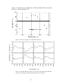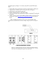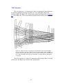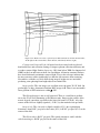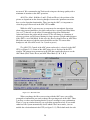
1
NOAO CCD MOSAIC IMAGER USER MANUAL
(KPNO Mosaic-1 Specific System)
Version: 3.0 September 1, 2004
Revision by Heidi Schweiker and Buell T. Jannuzi
of the September 15, 2000 version written by George Jacoby
With contributions from
Taft Armandroff, Todd Boroson, Jim De Veny, Steve Heathcote,
Tod Lauer, Bob Marshall, Phil Massey, Rich Reed, Frank Valdes, David Vaughnn
The Veil Nebula (courtesy Travis Rector, Univ of Alaska Anchorage) as observed
with the WIYN 0.9-m telescope and Mosaic-1
[send comments on manual to [email protected] or [email protected]]
1
Table of Contents
1. Mosaic-1 Overview: At Least Read This!....................................................................................................................4
2. Introduction ....................................................................................................................................................................8
2.1. Instrument Overview.....................................................................................................................8
2.2. Philosophy and Structure of Manual...........................................................................................8
2.3. Supplemental Information: Other manuals and Web pages to look at...................................9
3. The Mosaic Hardware .................................................................................................................................................10
3.1. The Mosaic CCDs .........................................................................................................................10
3.2. The Dewar .....................................................................................................................................12
3.3. The Arcon Controllers .................................................................................................................12
3.4. The CCD Shutter...........................................................................................................................13
3.5. The Filter Track.............................................................................................................................14
3.6. Filters For Mosaic .........................................................................................................................14
3.7. Operation of the Guider TVs ......................................................................................................19
3.8. Correctors ......................................................................................................................................21
3.9. Atmospheric Dispersion Corrector (at the 4-m only) ..............................................................23
4. Software.........................................................................................................................................................................26
4.1. Logging in and firing up the Arcon/Mosaic software............................................................26
4.2. Autologging ..................................................................................................................................28
4.3. Restarting the Arcon software ....................................................................................................28
4.4. Restart and Power Cycling of the Arcons and Nexus/Tram box..........................................28
4.5. Shutting down the software and Logging out .........................................................................33
4.6. OBSINIT.........................................................................................................................................33
4.7. Re-starting the MSE and related software ................................................................................34
4.8. Observe - The Only Command You Really Need to Know....................................................35
4.9. Exposure Control Commands ....................................................................................................37
4.10. Other Commands For Taking Data..........................................................................................37
4.10.1. Taking exposures of specified type..............................................................................................37
4.10.2. Getting more of the same............................................................................................................38
4.10.3. Taking a test exposure ................................................................................................................38
4.10.4. Taking your flats the easy way...................................................................................................38
4.10.5. Grids and Dithering...................................................................................................................39
4.11. Controlling the Data Capture Agent (DCA) on Tan or Emerald .........................................42
4.12. Observing in Binned Mode .......................................................................................................44
5. Evaluating, Recording, and Reducing Mosaic Images ...........................................................................................47
5.1. Working with Mosaic Data Files ................................................................................................47
5.2. Displaying and Evaluating Images at the Telescope...............................................................48
5.3. Examining the Data......................................................................................................................50
5.4. Recording Mosaic Data................................................................................................................52
5.5. The Reduction of Mosaic Images ...............................................................................................53
5.6. Calibration Data to Obtain At the Telescope ............................................................................53
5.7. Basic Reductions ...........................................................................................................................54
5.8. The Variable Pixel Scale and Zero Point Uniformity...............................................................54
5.9. Stacking Mosaic Images...............................................................................................................55
5.10. A Simplified Summary of the Processing Steps .....................................................................58
6. Appendix A: Miscellaneous Software Commands .................................................................................................59
7. Appendix B: Differential Refraction ..........................................................................................................................61
2
8. Appendix C: Issues About Photometry ....................................................................................................................62
9. Appendix D: Flat-Field Exposures ............................................................................................................................63
10. Appendix E: Frequently Encountered Problems (FEP) ........................................................................................64
10.1. Mysterious messages appear and pictures cannot be taken.................................................64
10.2. Data Doesn’t Show Up on Reduction Computer. ..................................................................64
10.3. "Echo" Images in adjacent CCD: "Cross-Talk"........................................................................64
10.4. Bad Rows in All CCDs...............................................................................................................65
10.5. Calibrating the CCD Voltages at the Start of a Block ............................................................66
10.6. The ADC does not seem to be reacting fast enough!.............................................................66
10.7. "Warning: ’ared’ package not defined" when starting ARCONS.........................................67
11. Appendix F: Rarely Encountered Problems ...........................................................................................................68
11.1. "Good" Error Messages..............................................................................................................68
11.2. "New" Errors as of September 2000 .........................................................................................68
11.3. Image display fails to complete automatically. ......................................................................69
3
1. Mosaic-1 Overview: At Least Read
This!
The Mosaic-1 and Mosaic-2 imagers are wide-field optical imaging cameras built for use
at Kitt Peak National Observatory and Cerro Tololo Inter-American Observatory. These
two cameras are nearly identical, but do differ in some respects. The operation of each of
these cameras (Mosaic-1 at the KPNO 4m and WIYN 0.9m; Mosaic-2 at the CTIO 4m)
also differ in some specifics. This manual contains much information that is common to
both cameras, but is focused on the specifics of using the Mosaic-1 at the KPNO 4m and
WIYN 0.9m
General Characteristics:
Arrays:
Pixels size:
Read-noise:
DQE:
Dark-current:
Read-out
time
(including
overhead):
CCD Gaps:
Cosmetics:
Filters:
Saturation:
Gain:
8 2048x4096 SITe CCDs; thinned , science grade
8192 x 8192 @ 16 bits, plus header, overscan:~135 Mbytes
15-um (0.26"/pixel at the 4-m; 0.43"/pixel at the 0.9-m)
~6 e−
86% peak at 6500Å (average for 8 CCDs; see also Figure 3.1.2)
~5 e−/pixel/hr
2 minutes 34 seconds (1 min 6 sec when binned 2x2)
~0.7 mm (~50 pixels) in rows; ~0.5 mm (~35 pixels) in columns
Good to excellent: typically 2 bad columns per CCD, but many
2-8 pixel areas of 5% variation (flatfield completely) and some
very large areas of 10% variations that all flatfield to <0.5%
5.75"x5.75"; parfocal,34 filters now available at KPNO (a list
of all available filters can be found here
http://www.noao.edu/kpno/mosaic/filters/filters.html) (UBVRI;
see Sec 2.6)
Typically, linear to 0.1% to 70,000 e~3 e−/ADU
4
KPNO Mayall 4-Meter Parameters:
Count Rates:
FOV:
Scale:
Image quality:
Artifacts:
Typical focus:
ADC:
At UBVRI=20th mag: U: 35; B:330; V: 340; R: 410; I: 225 e/sec
36’x36’, XIMTOOL Orientation: North- left, East-down
0.26"/pixel at center; decreases quadratically by 6.5% out to
corners
PSF quite constant across the FOV, but ~6% larger in linear
scale at the corners
Faint ~2600-pixel wide image of the pupil in each image (~1%
at UI, 0.8% at BVR, 2-4% in narrow-band filters).
-9900 at ~17C (-10200 for U; approximately -300 unit offset
for U-band); change with temperature: -90 units per degree C
Atmospheric Dispersion Correction: For broad-band filters,
use ADC in "track mode" with appropriate filter selected. For
flat-fields and narrow-band exposures, use the "null" position
or closest broad-band filter mode in wavelength.
WIYN 0.9-Meter (formerly KPNO 0.9m) Parameters:
Count Rates:
FOV:
Scale:
Image quality:
Typical focus:
At UBVRI=20th mag: U: 2; B: 14; V: 15; R: 16; I: 9 e-/sec
59’x59’, XIMTOOL Orientation: North-left, East-up
0.43"/pixel
PSF fairly constant across the field, but a 20-30 focus unit tilt
is present.
31000 at 10C (31050 for U); change with temperature +80 units
per degree C.
Data Acquisition: Acquisition commands are given on computers named rush (at
KP4m) or rust (at W0.9m). These computers are currently accessed by the user via a
VNC display on tan (at KP4m) and emerald (at W0.9m).
Data Reduction: At the KP4m images can be inspected and processed using the
computers tan or nutmeg. At the W0.9m this work is done on emerald.
5
All the Commands That Are Likely To Be Needed
Observing Commands -- on Rush (at KP4m) or Rust (W0.9m)
observe
doobs
mosdither
more
test
object
zero
dark
dflat
sflat
focus
recover
take one or more exposures prompting for the exposure type
a script which takes flats/objects for a list of filters
takes (typically 5) dithered images in a single filter to fill the
gaps in array
take more exposures just like the last one
take a test exposure. The output image, test, is overwritten each
time
take one or more object exposures
take one or more zero (bias) exposures
take one or more dark exposures
take one or more dome flats
take one or more sky flats
take a focus frame
recover data (if possible) following a crash of the DCA during
readout
Exposure Control Commands
pause
resume
tchange
stop
abort
pictitle
pause exposure (e.g. clouds) [do not ABORT or STOP from
within pause!]
Resume a paused exposure [then ABORT or STOP if
necessary!]
increase or decrease the exposure time
stop an exposure (and sequence of exposures) reading out the
detector
abort an exposure (or sequence) discarding the data
Change the title of the picture
Quick-look and Taping Commands -- on Tan (at KP4m) or Emerald (W0.9m)
Mscdisplay
Mscexamine
Mscwfits
display an entire mosaic frame
general tool for examining images
write mosaic frames to tape in multi-extension FITS format
Caution: Tape your data as you go; DLT-7000 (~250 images/tape) and Exabyte drives
(~35 images/tape), and DDS-4 DAT drives (~145 images/tape) are available. On nutmeg
(KP4m) it takes the following times to write/read images using mscwfits: DDS-4 DAT
49/54 sec, Exabyte 1:29/1:14, DLT (no compression) 0:37/1:02). DVD writer (4 GBytes)
and CD/RW are also available. Please be off the computer by noon of your last day!
You can purchase DLT, DAT and Exabyte tapes as well as DVDs (DVD-R 4x) at the Kitt
Peak Administration office, but bringing your own is cheaper.
6
Calibration data:
If you wish, take darks matching expected exposure times, although we have not
measured significant dark current with the current version of the instrument.
Take dome flats and/or twilight flats (night sky flats work even better!)
Take zeroes (i.e., biases) -- Darken the dome for darks and zeroes!
7
2. Introduction
2.1. Instrument Overview
The NOAO CCD Mosaic cameras are wide field imagers having 8192 x 8192
pixels. At the KPNO 4-m, where the pixels are 0.26" on the sky, this provides a field
of view of 36 arcmin on a side. At the WIYN 0.9-m, where the pixels are 0.43" on
the sky, the field of view is 59 arcmin on a side.
Each unbinned exposure with the camera requires 2:34 of over-head (including
exposure preparation time and CCD readout). When used with binning, the readout
time for MOSAIC is reduced but the preparation overhead remains. When used with
2x2 binning the total exposure over-head is 1:06. The CCDs are read out through 4
Arcon controllers to a data taking computer (known as rush at the 4-m and rust at
the 0.9-m), which serves as an intermediary data gateway. The pictures really end up
on a faster computer (known as emerald at the W0.9-m and tan at the KP4-m)
where you can display and examine the data, perform full reductions, and tape the
data much more effectively. Rush and Rust should be used only to do the minimal
work required to take observations because the data rate through it is tremendous and
nearly pegs the CPU at 100%.
Pictures are 135 Mbytes each. A typical night of ~70 pictures produces about
10 Gbytes. Be aware that processing this data, even just reading it, is a major task for
many computing systems. We recommend using a DDS-4 or DLT tape; however, we
provide Exabyte 820 (8505XL compatible) drives for those who do not have DDS-4s
or DLTs. Provide enough time to tape your data each night. With the Exabytes, an
image takes ~1min20sec to tape using tan, so 70 pictures will take nearly 2 hours
even without a verification pass. We also offer DDS-4 DAT, DVD and CD/RW at
both telescopes.
The Mosaic cameras require large (5.75 inch) filters to avoid vignetting. We
can provide an adapter for 4 inch filters, but using them makes poor use of the
Mosaic’s wide-field.
2.2. Philosophy and Structure of Manual
This manual was originally intended for an observer planning to use either of
the NOAO CCD Mosaic imagers. It is not intended to serve as a hardware or
software reference document describing the inner working of the Mosaics, although
some details at that level are present to help the observer plan observing strategies.
Also, we assume that the observer is already familiar with CCD cameras,
observations, and reducing data. The current versionis Mosaic-1 centric, i.e. focused
on the Mosaic camera available at KPNO.
8
Two very brief summary pages are at the front of this manual. If you’ve read
this far, and don’t plan to read any further, be sure you understand those 2 pages.
Development of the Mosaic systems is a continuing process, although only
very minor adjustments are being made at this time. Throughout the lifetime of the
instruments, filters will be added, old ones replaced, and software enhanced. This
manual represents the status as of the date on the cover page. We expect to revise the
manual occasionally to include information gained during engineering runs, as well
as to reflect new filters.
This manual also appears as an HTML document on the NOAO WWW pages
(http://www.noao.edu/kpno/manuals). It can be downloaded as a PDF file via
anonymous FTP to ftp.noao.edu, cd kpno/manuals, binary, get mosaic_man.pdf. We
welcome suggestions for improving this manual.
2.3. Supplemental Information: Other manuals and Web pages to
look at
Other useful information regarding the use of the Mosaics, CCDs, and
observing and reduction software can be found at:
NOAO Mosaic Camera web pages
(http://www.noao.edu/noao/mosaic)
Direct Imaging Manual (http://www.noao.edu/kpno/manuals/dim/dim.html)
NOAO/KPNO Mosaic Web Page
(http://www.noao.edu/kpno/mosaic/mosaic.html)
NOAO/CTIO Mosaic Web Pages
WIYN 0.9-m User’s Manual
(http://www.noao.edu/ctio/mosaic)
(http://www.noao.edu/0.9m/manual.html)
Buell Jannuzi’s Reduction Guide
(http://www.noao.edu/noao/noaodeep/ReductionOpt/frames.html)
Various Publications (SPIE, ADASS, ?)
Mosaic Data Handling System (Valdes 1998, SPIE 3355, 497)
(http://www.noao.edu/noao/meetings/spie98/mdhs.ps)
CCD Detector upgrade for NOAO’s 8192 x 8192 Mosaic (Wolfe 1998, SPIE 3355, 487)
(http://www.noao.edu/noao/meetings/spie98/wolfe.html)
What is better than an 8K x 8K Mosaic? (Muller 1998, SPIE 3355, 577)
(http://www.noao.edu/noao/meetings/spie98/muller.ps)
A New Wide Field Corrector for the Kitt Peak Mayall 4-m (Jacoby 1998, SPIE 3355,
721)
(http://www.noao.edu/noao/meetings/spie98/jacoby.ps)
9
3. The Mosaic Hardware
3.1. The Mosaic CCDs
The Mosaic Imager features eight 2048 (serial or pixels/row) x 4096 (parallel
or pixels/column) 15 µm pixel CCDs arranged as an 8192 x 8192 pixel detector. The
Mosaic-1 CCDs are read out through a single amplifier per chip simultaneously to 8
controller inputs (on 4 Arcon controllers). For Mosaic-2 (at CTIO) 16 amplifiers, 2
per CCD, are working and can be readout simultaneously. Unfortunately, two of the
CCDs in Mosaic-1 only have one working amplifier, limiting Mosaic-1 to work in 8
channel mode. The resulting mosaic array is a square about 5 inches on an edge. The
gaps between CCDs are about 0.7 mm in the row direction and 0.5 mm in the
column direction. [See Figure 3.1.1 showing an image labeled with chip numbers.]
The Mosaic Imager is populated with thinned, AR coated SITe CCDs. These chips
have only minor flaws that have little effect on their scientific performance, but they
do require careful calibration to attain excellent flat-fielded images.
Figure 3.1.1: A Flat-field (R band) map of the CCDs in the Mosaic with their ’extensions’
(im1, im2, im3, ?) as used in the IRAF nomenclature (see section 5).
10
Figure 3.1.2 shows the average QE for the 8 CCDs. Individual CCDs deviate from
this curve as shown in Figure 3.1.3.
Figure 3.1.2: The average QE for the 8 SITe CCDs in Mosaic I.
Figure 3.1.3: The QE differences relative to the average for the 8 SITe CCDs in Mosaic I.
Also shown are the readnoise (RN) and gain (GN) values for each CCD.
11
3.2. The Dewar
The Mosaic dewar is a large (6.3 liter) vacuum vessel radiatively coupled to
the CCD mount. It is the large round cylindrical object in the center of Figure 3.2.1.
The hold time of the dewar is 17 hours. It is filled by an observing technician at the
start and end of each night.
Several temperatures within the dewar are monitored and displayed in the
Mosaic Graphical User Interface (GUI).The CCDs should be between -83 and -98 C.
The dewar tank is cooled to -166 C or cooler. A good way to detect the exhaustion of
LN2 is the warming of the ’fill neck’ temperature, which is normally near 0 C. If this
temperature begins to rise much above zero or any of the temperature boxes turn and
stay red, call for assistance to have the dewar filled. Mosaic automatically e-mails
mountain personnel if various temperatures rise to levels that indicate a warm-up.
Figure 3.2.1: The Mosaic system mounted at the back of the 0.9-m telescope. The dewar containing
the 8 CCDs is the silvery, cylindrical object in the middle. It is surrounded by the filter track, which is
housed in the large black oval that extends horizontally across most of the picture.
3.3. The Arcon Controllers
The eight CCDs are read out through four Arcon controllers. These controllers
run at 100 kpix/sec per CCD, yielding a readout time, including all overheads,
of~2min34sec for Mosaic-1 (only a single amplifier is used). Data values are stored
as 16-bit unsigned integers. For further details about the Arcon controller systems,
see the technical paper by Roger Smith
(http://www.ctio.noao.edu/instruments/arcon/arcon.html).
The data taking computer (rush or rust) is a 125 Mhz Sun Sparcstation 10
running SunOS. It has sufficient resources to manage the data acquisition, but not
12
much more. The large data volume is handed off to the reduction computer (tan
(KP4m) or emerald (W0.9m)) via Fast Ethernet for all analysis and reductions,
thereby relieving rush/rust of unnecessary loads. These are fast Linux boxes with
>100 Gbytes of disk and >1 Gbyte of RAM.
Figure 3.3.1: A view of the Mosaic system on the 0.9-m telescope indicating 2 of the 4 Arcon
controllers. Also the south guide TV housing can be seen, as well as the Mosaic dewar (now
appearing in black).
3.4. The CCD Shutter
The shutter consists of a pair of opposing sliding blades, one of which has
rectangular slots open for the guide field. The blades are attached to pneumatically
driven cylinders to provide very fast control of the shutter. This design allows the TV
guide fields to be shuttered independently of the science field. In the guide mode, the
closed shutter still allows the TV guide cameras to see the sky. In the dark mode,
these fields are closed as well. The acquisition software controls which mode the
shutter remains in between exposures. For object observations, the shutter goes to the
guide mode before the exposure begins. For requested observation types of dark, flat,
or zero, the shutter goes to the dark mode before the exposure begins (and remains in
this mode after the exposure and readout are completed).Note that the TV fields are
always open when the shutter is open; the different shutter modes only control the
TV fields when the science shutter is closed. If you have been taking darks, flats, or
13
zeros, you may need to set the shutter mode to guide in order to get light to the TV
guide camera.
The time for the blades to move completely across the field is 23 msec. The
motion of the blades during both opening and closing are in the same direction so
that the exposure level is nearly constant over the array. The motion of the shutter
blades is along columns. The accuracy of the shutter has been measured to be ~3% in
a 1-second exposure (that is, the exposure is really 0.97 seconds; see also Section 8).
3.5. The Filter Track
The filter track holds 14 filters. For each filter position, there is a filter for the
CCD field, and two separate filters for the two TV fields. Separate filters are used so
that a narrow bandpass science filter does not constrain the observer to find very
bright guide stars. Normally, one would use clear (BK7) filters for the TV, but one
can use a red filter to minimize moonlight or match the science filter more
accurately. One might want to match the science filter, at least approximately, to
minimize a guider drift. Even at the 4-m, residuals after the correction from the ADC
are of order 0.1-0.2 arcsec. This, and all filter decisions, must be made ahead of time,
as the filters can only be changed during the day by a qualified observing technician.
Adapters exist to allow the use of 4-inch-square (1 adaptor) and 2-inch-square
(2 adaptors). At the 0.9-m (f/7.5), these 4-inch filters illuminate approximately 6K X
6K pixels (56% of the total sky area); At the 4-m, 4-inch filters illuminate
approximately 5.5K X 5.5K pixels (46% of the total sky area).
The positioning of the filter track is highly repeatable. However, the
acceleration of the track can occasionally dislodge dust particles between filter
moves, particularly if intervening movements have turned the filter upside down. In
all cases, the filter track software moves the track in the direction that minimizes the
distance moved to reach the requested filter position.
In addition to the 14-position filter track, there is a manual slide that can hold a
single filter of the same size (5.75 inches square).This may be used, for example, to
hold a bandpass filter when polarization filters are used in the track. Use of an
additional ’hand-insert filter’ changes the focus. At the 4-m, changing, inserting, or
removing this filter can only be done at the maintenance (Southeast Annex) position.
3.6. Filters For Mosaic
To fully utilize the field of view of the 8Kx8K, filters must be 5.75 inches (146
mm) square, and have 5.43 inches (138 mm) clear aperture. The optimum thickness
that preserves image quality over the entire field of view is 0.47 inches (12.0 mm).
All NOAO mosaic filters adhere to these specifications to maintain a parfocal
condition. Thus, neither the telescope nor the guide TVs should require a focus
change when switching between filters. There is one exception, the CuSO4 U filter
14
(k1001), for which there is a focus offset. Some of the currently available filters and
approximate count rates (e−/sec) for a 20th mag star are:
4-m
Filter
U
B
V
R
I
H
H +4
H +8
H +12
H +16/[SII]
SDSS g’
SDSS r’
SDSS i’
SDSS z’
[OIII] #2
[OIII]+29#2
White
Wash M
Wash C
DDO 51
WR CIII
WR HeII
WR 475
WR CIV
TV
S8612
BG38
BK-7
RG610
BK-7
BK-7
BK-7
BK-7
BK-7
BK-7
BK-7
BK-7
BK-7
BK-7
BK-7
BK-7
BK-7
BG38
S8612
BK-7
BK-7
BK-7
BK-7
BK-7
−
0.9-m
FWHM
e−/s
35
330
Central
Wave
3577
4360
647
990
2
14
940
1510
340
410
5370
6440
940
1510
15
16
8220
6569
6611
6650
6692
6730
4813
6287
7732
9400
5021
5305
5600
5100
1930
80
81
81
81
80
1537
1468
1548
2000
55
241
6800
1140
225
8220
~6575
~6615
~6656
~6695
~6736
4813
6287
7732
9400
~5027
~5305
5600
5100
1930
~80
~81
~81
~81
~80
1537
1468
1548
2000
~53
241
6800
1140
9
3860
5132
4653
4690
4750
~5816
1034
161
52
51
51
46
3860
~5132
~4660
~4695
~4755
5823
1034
161
~50
~49
~49
42
Peak
T%
79.5
69.3
Central
Wave
3577
4360
FWHM
e /s
646
990
88.4
86.2
5370
6440
93.9
94.3
91.2
89.5
86.1
90.7
90.2
91.8
94.6
94.8
75.2
90.5
97.2
87.1
75.4
85.1
68.4
73.3
78.8
72.7
15
See Figures 3.6.1 through 3.6.5 for plots of the current filter transmission
curves. ASCII Tables that describe the transmissions are available on the Mosaic
Web Pages.
The U-band filter is based on the same formulation as our 4" filter set (liquid
CuSO4 + UG-1). Because containment of the liquid requires a thickness around the
edge that exceeds the nominal Mosaic dead zone, some vignetting is present. At the
4-m, the vignetting introduces a 20% loss of light at the edge, but recovers to zeroloss at 200 pixels from the edge.
Figure 3.6.1: The broad band filter set, including the ’White’ filter.
16
Figure 3.6.2: The SDSS g’, r’, I’, and z’ filters, along with Washington C and M (M is the smooth
curve slightly redder than g’).
Figure 3.6.3: The current set of H (plus redshifted) filters. Note that H +16 serves as a [SII] filter.
17
Figure 3.6.4: The blue Wolf-Rayet filters for [CIII], He II, and a continuum at 4750.
Figure 3.6.5: The [OIII] on-band and off-band filters, plus DDO 51.
18
Figure 3.6.6: The V-band filter installed in the filter track. The 2 TV guider filters are
visible to the lower left and upper right of the science filter. An Arcon controller can be
seen in the background to the right.
3.7. Operation of the Guider TVs
Guiding with the Mosaic is accomplished using one of two TV cameras on the
north and south sides of the science field. These are intensified fiber-optically
coupled CCD cameras ("ICCDs"), and so, they can be damaged if exposed to bright
light. The video signal from the selected TV camera is fed to the guider system. The
field of view of each camera is about 2.2 arcmin on a side at the 4-m and about 5
arcmin on a side at the 0.9-m.
The field of view of the TVs is fixed with respect to the science field. At the 4m, the fields are approximately 1440 arcsec north and south of the center of the
science field. At the 0.9-m, the fields are approximately 2400 arcsec north and south
of the center of the science field. TV focus can be moved remotely; offsets are -0.9
and -1.7 at the 4-m, and -0.1 and -1.9 at the 0.9-m, for the north and south TVs,
respectively.
At a given location, suitable guide stars are almost always available without
moving the telescope from the desired position. We find that we can guide at the 4-m
on stars as faint as V=20 in full moon, and at the 0.9-m to V~17 near full moon.
The TVs and guider are controlled by the telescope operator at the 4-m, but by
the observer at the 0.9-meter.The observer needs to first select the N or S TV on the
19
distribution panel (see Figure 3.7.1). For the selected TV, on the ICCD Control
Panel:
1.
2.
3.
4.
5.
Turn the high-voltage potentiometer completely counterclockwise (10 turn pot)
Toggle the power switch on (on TV screen, pixel defects will appear)
Neutral density switch should be down (off)
Push the momentary button to enable high voltage
Slowly turn the high voltage potentiometer clockwise, monitoring TVs until guide
stars appear
6. Acquire a guidestar on the computer moss and initiate guiding (consult the 0.9-m
telescope user’s guide (http://www.noao.edu/0.9m/Tel_Op.html) for details on
step 6)
When switching between the two TVs, be sure to turn the high voltage
potentiometer counterclockwise and turn off high voltage on the TV no longer in
use.
Figure 3.7.1: A schematic drawing of the layout of the TV control panels at the 0.9-m.
Only the two leftmost panels in the lower rack are used with the Mosaic TVs. The upper
rack is used to select which TV/video signal is seen on the monitor.
20
3.8. Correctors
The 4-m corrector is a 4-element fused silica (for maximum U-band efficiency)
design with additional internal prisms that serve as an atmospheric dispersion
corrector (ADC). See Figure 3.8.1 below for the optical layout and refer to Jacoby et
al. (1998, SPIE 3355, 721) for a detailed description of the corrector and ADC.
Figure 3.8.1: The 4-m corrector optical layout. All elements are made from fused silica
except for the ADC components, which are made from LLF6, UBK7, LLF6, and UBK7 as
viewed from left to right. At the right are the science filter, dewar window, and CCD (from
left to right). The ADC elements appear in the middle as 4 planar elements (although they
are wedged).
The 0.9-m corrector is a simple 2-element fused silica design. There is no ADC
at the 0.9-m. See Figure 3.8.2 below for the optical layout.
21
Figure 3.8.2: The 0.9-m corrector optical layout. Both elements are made from fused silica.
At the right are the science filter, dewar window, and CCD (from left to right).
Coatings and Scattered Light: All optics have been coated with very broadband multi-layer anti-reflection coatings to improve photon collection efficiency and
to reduce scattered light. Surface losses are ~10% from below 3500 Å to longward of
9500 Å at the 4-m and better at the 0.9-m. In addition, all interior structural surfaces
have been blackened to minimize scattered light. Tests at the telescope indicate that
the new correctors suffer significantly less than the old correctors from scattering.
Nevertheless, with the very wide fields being imaged, bright stars are inevitable,
producing some ghosting from bright objects in certain fields.
Image quality: The 4-m images are excellent across the entire 35'
x35'field. On
good nights, we have documented uniform 0.65'images in R. There is no measurable
focus gradient or PSF variation to within ~10%.
The 0.9-m telescope is not as well corrected. There is a small focus gradient
across the 59'
x59'field amounting to 20-30 focus units. Images in the corners of the
mosaic degrade somewhat, especially in the lower-left corner (CCD #1). Also, the
corners of the field are slightly vignetted (~5-10%) by the internal telescope baffle.
Image Scale: The 4-m scale is slightly variable (6.3%) due to pincushion
distortions, from 0.261" per pixel at the center (f/3.1) to 0.245" per pixel (f/3.3) at the
corner of the field.
The 0.9-m scale is 0.425" per pixel. The spatial variation is small, with the
scale decreasing to ~0.420" per pixel at the corner of the field.
22
Ghost Pupil: When using narrow-band interference, very blue (e.g. U) or red
(e.g. I, z’) band filters at the 4-m, a faint image of the telescope pupil falls on the
CCD and has a diameter of about 10 arcmin. Depending on the bandpass and
construction of the filter, this reflection typically manifests itself at <1% for broad
band to 2-4 %(narrow-band [OIII], Hα, U, I, z’) level above the background. It arises
from an internal reflection off the front surface of the rear element of the corrector
despite the use of an extremely good anti-reflection (AR) coating. Our investigation
suggests that similar 4-element correctors currently in use should exhibit a similar
effect, and tests performed by Alistair Walker with the CTIO 4-m confirm this
analysis.
Although the ghost pupil can subjectively appear severe when viewed at high
contrast (for narrow-band filters), photometric accuracy is preserved when this
additive term is removed during the reductions. One can avoid the affected region on
the Mosaic array by moving the telescope slightly if there is any concern about the
reduction process [see Sec. 4].
For a description of how to correct for pupil ghost images in your observations
you can read the discussion in the NOAO Deep Wide-Field Survey MOSAIC
Reduction Cookbook
(http://www.noao.edu/noao/noaodeep/ReductionOpt/frames.html).
3.9. Atmospheric Dispersion Corrector (at the 4-m only)
The Earth’s atmosphere disperses the light from stars significantly when
observing away from zenith. The effect is greatest and similar at U and B where the
stellar image is stretched, for example, ~0.5" at a zenith distance of 45° (1.4
airmasses), and 0.9" at 60° (2 airmasses). The ADC prisms can be configured via a
rotation to counter this effect nearly completely, thereby greatly reducing the
elongation of the image introduced by the atmosphere.
Modes of Operations: There are 3 modes that the ADC system can be used1.
Null mode, where the ADCs make no correction; Track mode, where corrections are
periodically updated; and, Preset mode, where the corrections are preset at the
beginning of an exposure to be correct for the middle of the exposure, but otherwise
1
The 3 ADC modes in more detail are:
1. Null Mode: The ADC prisms are set to a fixed position that makes no correction
for the
atmosphere.
2. Track Mode: The positions of the ADC prisms are automatically updated at a
periodic rate (typically, 60 second intervals) to account for the changing zenith and azimuth
directions of the telescope as it moves (e.g., as it tracks during an observation or slews to a
new position).
3. Preset Mode: The positions of the ADC prisms are set to a pre-determined
location as demanded by the mid-point of the exposure. In this mode, movement of the
ADC prisms is synchronized with the data acquisition sequence. In this mode, the ADC
prisms do not move during the exposure.
23
not moved. We recommend using Track mode to improve the image quality with a
minimum of attention to the ADC operations.
ADC Filter Mode: In Modes 2 and 3 (Track and Preset), the positions of the
prisms are dependent on the observing bandpass because the optimum corrections
have a color-dependent functionality. Thus, in using the ADC, it is important to
select the proper filter mode in the ADC GUI on rush.
While the ADC is not necessary to compensate for atmospheric dispersion
when using narrow-band filters, the guide cameras have separate broad-band filters
[see sec 2.7] that will see the effects of atmospheric dispersion. Differential
refraction between the guider and the science CCDs will change as a function of
telescope position, and will cause blurring for long exposures at high zenith distances
if the ADC is set to Null Mode. In this case, the observer should select an ADC Filter
Mode that encompasses both the narrow-band filter and the TV camera filter
bandpasses and select ADC mode 2 or 3 (track or preset).
The ADC GUI: Control of the ADC prisms and modes is selected via the ADC
GUI (see Figure 3.9.1). Status of the ADC prisms also is displayed in the GUI
window. The primary user parameters in the GUI that concern the observer are the
ADC Mode (Null, Track, Preset) and ADC Filter Mode (U, B, V, R, I).
Figure 3.9.1: The ADC GUI.
When you change the filter you are using with the ADC in use you will be
prompted to confirm that you want to change the operating mode of the ADC. There
is no beep, or other sound warning that the system is waiting for your confirmation.
There is a pop-up window that asks you to pick the appropriate mode. If you would
rather have the system automatically decide which is the correct mode, you can
unclick the selection button in the GUI (see figure 3.9.1). The default mode for each
24
filter is listed at http://www.noao.edu/kpno/mosaic/filters/filter_names. Note that the
default of start-up mode of operation is for the system to prompt the observer to
confirm the ADC mode before starting the first observation with a new filter.
25
4. Software
4.1. Logging in and firing up the Arcon/Mosaic software
Before you can begin to take data you must log in on both the data acquisition
(rush/rust) and data reduction (tan/emerald) computers. We are currently
controlling the Mosaic-1 with rush (KP4m) or rust (W0.9m) with the data handling
and analysis being done with tan (KP4m) or emerald (W0.9m). Both emerald and
tan have 3 monitors labeled tan/emerald:0.0 (center monitor), tan/emerald:0.1 (left
monitor), and tan/emerald:0.2 (right monitor). At the 4m there is an additional data
reduction computer, nutmeg, which has a dual processor. Note that the home
directory for tan is /md1/4meter and on nutmeg is /md4/4meter.
0.9m.
To begin your observing session you should follow these steps at either the 4m or
1. Log on to tan (emerald) as user 4meter (36inch). The computer tan is a fast
computer with two CPUs (1.667 GHz AMD processors) and 1 Gbyte of memory
operating under Linux. The computer emerald is also a fast Linux box with a 3.4
GHz (Pentium 4) CPU and 2 Gbytes of memory.
2. On the central console (tan:0.0 or emerald:0.0) right click on the background to
bring up the menu of options. The top option is "Start Interfaces for MOSAIC
CCD". Select this option. This will open the VNC2 client in tan:0.1 (or
emerald:0.1) in which the windows from rush (or rust) will be displayed. It will
also start the DCA (Data Capture Agent) and associated GUI of the data handling
system in the center monitor (tan:0.0) as well as the Ximtool display in tan:0.2 (or
emerald:0.2), displayed on the right monitor. The right monitor is only an 8-bit
display (to accommodate the current version of X-imtool; a new version with 24bit color is under development) and should only be used for the display window
or there will be problems with the allocation of colors to the display window. We
are still working out some undesirable features in this display. If you would rather
use DS9 as an option for the image display, kill the Ximtool window, right click
on the background of tan:0.2 to bring up the menu, and select DS9. DS9 should
work fine as your display device. If you want to switch back to Ximtool, you will
have to log out of tan and then log back in and restart as described above. This
2
VNC stands for Virtual Network Computing, a software program that allows one to view and
manipulate windows on another computer. We use VNC to remotely view the Arcon control
computers (rush at the 4m and rust at the 0.9m). For more information on VNC see
http://www.realvnc.com.
26
will not affect the operation of rush, but should not be done when you are reading
out an exposure or you will lose that exposure.
3. In the VNC viewer window on tan or emerald, click in the background of the
display and select (Re)START ARCONS. This should bring up all of the
MOSAIC GUI’s controlled by rush (rust).
This process takes about 2 minutes and you must also answer one question. A
small window labeled "ARCON Console" will appear near the left center of the
screen in which various messages will scroll by. After a few seconds a larger
window labeled "ARCON Acquisition" will open immediately below this; this is the
window you will use for entering all data acquisition commands. A brief greeting
message will appear in this window and, eventually, you should be asked
Do you want to synchronize parameters? (yes)
When you reply "yes" (or just hit [cr]), the detector parameters loaded into
Arcon will match those stored in detpars and the positions of the motors recorded in
instrpars will correspond to reality. We currently recommend saying yes at the start
of an observing run, but "no" during subsequent restarts. This saves slightly on the
start-up time. In either case the IRAF package menus will be printed and the cl>
prompt will appear. Some further windows will also pop up at this point. The system
is now ready for you to begin observing.
Occasionally things will get hung up during the process of downloading and
initializing the Arcon software. If this happens you may see the message (but
probably not)
****************************************
**
*FAILURE DURING ARCON STARTUP !!!*
**
*Use re-start button to try again*
**
****************************************
In the majority of cases, simply performing the restart procedure will fix this
problem, although it may be necessary to try this more than once. If after repeated
attempts the system will not start, refer to the Frequently Encountered Problems
section for further advice.
•
Right click on the background of TAN:0.0 (or Emerald:0.0) and select (Re)start
DCA. When you started ARCONS on rush (rust), the start-up procedure will
27
have killed the previously started DCA. You can restart the DCA right after you
start the ARCONS on rush (rust), you do not need to wait until the ARCON
start-up has completed.
The system is now ready for you to start observing.
4.2. Autologging
If you would like to use electronic auto-logging of your observations, you will
need to follow the instructions here (http://www.noao.edu/kpno/manuals/aol),
including running loginit in a data-reduction window on tan (or emerald)
4.3. Restarting the Arcon software
Every so often, something or other happens which causes the Arcon software
to hang, or otherwise get confused. In the vast majority of cases this can be fixed by
simply restarting the software running on rush/rust. This takes only a couple of
minutes.
•
On rush/rust (inside the VNC window on tan:0.1 or emerald:0.1): Move the
mouse pointer to an empty section of the desktop and hold down the right hand
button to bring up the desktop menu. Select the item "End ARCON Session" and
release the mouse button. After a few seconds the ARCON console, Acquisition,
status and countdown windows will disappear. Once the windows have
successfully closed, and the CPU meter has dropped to zero you can then restart
the Arcon Session. Again bring up the desktop menu via the right hand mouse
button and select "(Re)Start ARCON session". The software will go through the
startup procedure described in [4.1]. You should normally answer "yes" to "do
you want to synchronize parameters". This ensures that the detector parameters
and filter positions, etc. match those in use prior to the re-start. Any other
windows on the desk top will be untouched so any processes running in them
will be unaffected, and you can continue to work in these windows.
When you (Re)Start Arcons the DCA on tan or emerald will close. You will
need to restart it again. To do this, hold down the right hand button to bring up the
desktop menu and select "(Re)Start DCA" and release the mouse button.
4.4. Restart and Power Cycling of the Arcons and Nexus/Tram
box
Occasionally, the Arcon controllers get into a weird state. There are roughly 5
levels of severity with which the user can respond.
1) Restart the Arcons: Use the pull-down menu on the data taking computer
(rush/rust) to select End ARCON session. After the windows have successfully
closed and the CPU has returned to zero, select Start ARCON session from the
28
background pull-down menu. This will take a little while. It may take several (3-5)
Restarts to succeed. Always try at least 3 Restarts before proceeding to the next level
of severity listed below.
2) Logout and Restart the Arcons: End the ARCON session on the data acquisition
(rush/rust) computer and completely log out of the data reduction (tan/emerald)
computer. Log back in and select "Start Interfaces for MOSAIC CCD". This will
start the ARCON session, DCA, and Ximtool-alt. If there are still problems starting
the ARCONs go to level 3.
3) Try some diagnostics: open a Unix window on the Data Acquisition computer,
and then run the following diagnostic commands that check for communication with
the Arcons:
/xp/source/sun/bin/nexus0123
/xp/source/sun/bin/aset0123
These should complete normally for all 4 Arcons. If they fail to complete, try a
few more times. If the errors are persistent, power cycle the TRAM box (see figures
4.4.1). At the KP4m power cycling the TRAM box is done remotely (see below). At
the W0.9m this is done manually (see below).
REMOTE POWER CYCLING OF THE TRAM BOX (4M ONLY)
a) Open an xterm window on Rush.
b) Telnet 4m-nexus-power (140.252.52.74).
c) Log in as 4meter - enter the password.
d) This window will print some information. Type off 1 and confirm with Yes.
e) Count slowly to 50. Type on 1 and confirm with Yes.
MANUALLY POWER CYCLING OF THE TRAM BOX (0.9M
ONLY)
a) Locate the TRAM box in the computer room (see figure 4.4.1 below).
b) Turn the power on the TRAM box off, wait 30 seconds and turn the power
back on.
Try the "/xp" commands again. If the "/xp" commands succeed, then try
the following commands from a Unix window on the Data Acquisition computer.
This is a subset of the normal Arcon startup.
29
cd
arcon_user
This will take a few minutes and tries to bring up the Arcons completely, but
not the other windows (GUI, IRAF). If it fails the first time, try a few more times. If
it succeeds or fails, type "arsh stop" to exit the window. If successful, attempt
another Arcon restart. If it fails, try 3 more times. If you still cannot get arcon_user
to complete, go to level 4.
4) Reboot the data-taking computer (rush/rust):
a) End the ARCON session by selecting "End ARCON session" on the
Data Acquisition computer (rush/rust).
b) Open an xterm window from the background menu on rush/rust.
c) Type "reboot-rush" (at KP4m) or "reboot-rust" (at W0.9m).
d) Wait a couple minutes for the reboot to complete. While waiting, cycle the
power on the TRAM box (see the TRAM box power cycling procedures
above).
e) Restart the VNC client to rush/rust via the background menu on
tan/emerald and start the Arcons via the background menu "(Re)Start Arcon
Session".
f) You may have to execute the level 3 commands to make any progress.
g) At this point, it probably won’t hurt to restart the DCA on the data reduction
computer using the pull-down menu.
5) This is the most serious mode and it should be done with the cognizance of
NOAO personnel. This will be a total restart of the system. Follow the process in
item (4) above for the data-taking computer, but only through step (c). Then quit the
DCA on tan or emerald
AT THE 4-M it is possible to cycle power to the instrument and Nexus/Tram box
remotely:
a) From a UNIX prompt type telnet 4m-nexus-power. Use 4meter as the
username. The password is posted in the control room. To turn off the power to
the Nexus/TRAM box type off 1 at the prompt and confirm with Yes.
30
b) From another UNIX prompt type telnet 4m-pf-power. Use 4meter as the
username. The password is posted in the control room. To turn off the ARCON
power controller type off 1 at the prompt and confirm with Yes.
c) Slowly count to 50.
d) Turn on the ARCON power controller by typing on 1 at the prompt in the
4m-pf-power window.
e) Turn on the Nexus box by typing on 1 at the prompt in the 4m-nexuspower window.
f) If the system still fails to run, try steps (1-3) several times. If that fails, call
for help.
AT THE 0.9-M you will need to bring the telescope to zenith and cycle the
power on the instrument manually:
a) Power off the Nexus/TRAM box in the computer room (see figure 4.4.1).
b) Go to the instrument and power off the Arcons. There are 4 red power
switches located on a power plug strip (see figure 4.4.2). Wait 10 seconds.
Power on the 4 Arcons.
c) Complete step (4d) by powering the TRAM box on.
d) Log back into both computers to restart the Arcon and DCA software.
e) If the system still fails to run, try steps (1-3) several times. If that fails, call
for help.
31
Figure 4.4.1: The Arcon "TRAM" box with Power Switch noted. At the KP4m you
should not need to use this switch - see section 10.2.
Figure 4.4.2: The Arcon power strip with 4 power switches noted.
32
4.5. Shutting down the software and Logging out
During your run, you may wish to stay logged in continuously to maintain your
window environment, especially if you’ve taken some time to move and resize
dozens of windows. On the other hand some folks feel that a "clean" environment
makes for healthier observing, thus you may wish to log out at the end of every night
to reset any gremlins back to their initial conditions. In all cases, after your last night,
you should log out completely from both rush/rust and tan/emerald.
To log out of tan or emerald it is not necessary to shutdown Arcons - you can
simply close the VNC window. However one can first end the Arcon session on
rush/rust if desired.
•
On rush/rust: Move the pointer to an empty section of the desktop (in the rushVNC window) and hold down the right hand button to bring up the desktop
menu. Select the item "End ARCON Session" and release the mouse button.
After a few seconds the Arcon console, acquisition, status and countdown
windows will disappear. Any other windows on the desk top will be untouched
so any processes running in them will be unaffected, and you can continue to
work in these windows. Then close the VNC window by clicking the ’X’ in the
upper right-hand corner of the window.
•
On tan/emerald: select "Logout ’4meter’..." from the ’K’ start menu at the bottom
left corner of the screen.
4.6. OBSINIT
At the very beginning of your observing run, you should clean off all of the
previous observer’s images and files, and reinitialize all of the IRAF parameters to
their default values. This must be done separately on both rush/rust and
tan/emerald.
You, or the instrument assistant, can accomplish this as follows:
On tan (or emerald)
•
Log on using the observer login and password posted on the machine.
•
In the IRAF "Data Reduction" window, and any other IRAF sessions that may be
running, type logout. The window should vanish.
•
Select "Unix Xgterm" from the root menu. (Move the mouse to any blank area of
the screen, and hold down the right mouse button. Slide the mouse down to
"Unix Xgterm".)
•
In the new window, type obsinit and answer the questions appropriately.
33
On rush (or rust):
If an Arcon session is active on rush or rust,
•
Shutdown the Arcon session. (Move the mouse to any blank section of the
desktop and hold down the right hand button. Select the item "End ARCON
Session" and release the mouse button.
•
Log out of any IRAF cl sessions that may be running.
•
Select "Unix Xgterm" from the root menu. (Move the mouse to any blank area of
the screen, and hold down the right mouse button. Slide the mouse down to
"Unix Xgterm".)
•
In the new window, type obsinit and answer the questions
On rush (or rust):
If an Arcon session is not active on rush/rust,
•
Open a "xgterm" window in the VNC window for rush/rust.
•
At the rush UNIX prompt, type obsinit and answer the questions
The reason for the above procedure is that you cannot have IRAF running
during an obsinit because parameters will not be reset correctly. Make sure that you
have logged out of each IRAF window before running obsinit.
Note that the user has the option of selecting whether CNTL-z or CNTL-d will
be the default for an end-of-file command; the former is the standard at NOAO, but
the latter is the standard at many other places. If you simply wish to set all of the
IRAF parameters back to their default values, you may run this in the middle of your
observing run without losing any files.
4.7. Re-starting the MSE and related software
The software (MSE) which controls the instrument (filter track, TV cameras,
etc.) and the communications software which links everything together (MPGrouter) are normally started by support personnel when the instrument is installed on
the telescope. However, a restart may be necessary from time to time. If the MCCD
configuration screen shows ????? instead of numbers for the TV camera focus and
temperature readouts, then there may be a problem with this software.
rush% rsh taupe (at the 0.9-m, or cinnamon at the 4-m)
taupe% ps -ax | grep msmid
is it there ? no
taupe% start-msmid
34
4.8. Observe - The Only Command You Really Need to Know
All data taking can be done by using a single command: observe. This
command takes one or more CCD exposures, as in the following example:
cl> observe
Exposure type (|zero|dark|object|comp|pflat|dflat|sflat|focus)
(zero): obj
Number of exposures to take (1:) (1):
Exposure time (0.:) (0.): 300
Title of picture: M33 V
Filter in wheel one (B): V
Telescope focus (0.): -10200
Filter1 = VTelfocus = -10200.00000
Image obj022
Mosaic1 [1:8315, 1:8220] bin=[1:1], gain 1
cl>
Observation finished...
You will be prompted for all the information required which includes:
•
Exposure type: can be "zero" (sometimes referred to as bias), "dark", "object",
"dflat", "sflat" or "focus". Note that when selecting from a list of options like this
you may enter any unique abbreviation. Focus exposures, which are somewhat
special, are described fully below in taking a focus frame.
•
Number of exposures to take: a sequence of this number of pictures, all having the
same parameters, will be taken.
•
Exposure time: the integration time in seconds (which need not be an integer).
This parameter will not be requested in the case of exposures of type "zero" for
which it is 0.0 by definition.
•
Title of picture: this will be included as the title in the image header.
In each parameter query you are supplied with a default value, which you can
accept by simply hitting [CR]; these default values are just the previous entries. If
you make a mistake, or change your mind, you can abort the command during the
parameter entry stage by typing ctrl-c; the superstitious may enter the command flpr
at this point in order to ward-off the evil eye. For exposures of types other than
"zero" and "dark", you may also be prompted for the following parameters of the
instrument/telescope:
•
filter in wheel one: the required filter. Note that filters are specified by name,
rather than by their position in the filter wheel; the way this translation is set up
is described in wheel psets.
35
•
Telescope Focus: the telescope focus setting
You can control whether you will be prompted for these instrument-related
parameters during observations (see section on motor control). Once you have
entered all the necessary information, there will be a short pause while the motors in
the instrument are moved to the required positions and then your CCD exposure will
begin. A short message will be printed which includes the name of the picture which
will result. This name is derived from the exposure type by appending a running
number which is automatically incremented after each exposure (how this number
can be adjusted and alternate naming schemes are described in obspars). The image
will be created in the current directory (at the time the observe command was
issued).
The observe command terminates as soon as the exposure starts and you can
enter other commands in the IRAF acquisition window. While you could type any
IRAF command you like, we suggest you keep this window free for entering the
special exposure control commands.
The status window will keep you informed of the progress of your exposure.
As soon as the exposure starts the first line will change from
’CONTINUOUSLY_ERASING’ to ’INTEGRATING’ and the status window will
also show parameters of the exposure such as the picture title. A counter in the status
window, and more legibly the countdown window, will begin counting down the
time remaining in the exposure. Another counter will count up the dark time - the
time since the CCD stopped being erased. This will be slightly greater than the
elapsed exposure time due to overheads in the controller, and will of course be very
much longer if you paused the exposure.
When the exposure finishes, the CCD will be read out. The first line in the
status window will change to "READING" and the "buffers read" counter will
indicate the number of buffers of data successfully transferred to the Sun. The data is
initially written in the controller’s internal format to a spool file, but it is
automatically converted into a FITS format image on tan/emerald within a few
seconds of the exposure finishing. The end of each exposure is accompanied by
distinct sound from tan’s speakers.
If you requested that observe take only a single exposure, the message
"observation finished ....." will appear in the IRAF interface window as soon as the
readout is complete; things are then ready for you to start another exposure. If,
instead, you requested a sequence of several pictures, the next exposure will start
automatically. You may immediately examine or process the resulting image even
though the sequence is not complete. Note that the "pictures remaining" counter in
the status window shows how many exposures remain in the sequence. Once the
final picture has been readout, the message "sequence finished ......" will appear in
the IRAF interface window. Should you miss the end of sequence or end of exposure
message, note that the CCD is idle and things are ready for you to initiate new
exposures, whenever the top line of the status display reads
’CONTINUOUSLY_ERASING’.
36
4.9. Exposure Control Commands
The following commands can be used to modify an ongoing exposure:
•
pause - Pause the exposure e.g. while waiting out passing clouds.
•
resume - Resume a paused exposure.
•
tchange - Change exposure time. You will be prompted for the amount by
which to change the exposure, which may be positive or negative. If used
during a sequence the duration of the present exposure and all subsequent
exposures is changed.
•
stop - Stop the exposure early, read out the CCD and save the data to disk. If
used during a sequence, the sequence is also terminated.
•
abort - Abort the exposure. The CCD is not read out and any data collected
during the exposure is irrevocably lost. If used during a sequence, the
sequence is also terminated. Do not abort a PAUSEd exposure! - resume
first, or suffer serious consequences! (i.e., results in a hung system, which
will need a restart).
•
pictitle - If when entering the title you typed M31 when you meant M33 you
can use this command to give your image a new title.
4.10. Other Commands For Taking Data
4.10.1. Taking exposures of specified type
In addition to observe, there are specific commands to take one or more
pictures of each type:
•
•
•
•
•
dark - Take one or more exposures of type dark
dflat - Take one or more exposures of type dome flat
object - Take one or more exposures of type object
sflat - Take one or more exposures of type sky flat
zero - Take one or more exposures of type bias
Except, of course, for the exposure type, these commands take the same
parameters (and prompt for them in the same order) as does observe. Apart from
saving you entering that one extra parameter, use of these commands allows one to
set default parameter values, and also select which parameters are prompted for
according to picture type.
While we were having trouble taking bias sequences at the KP4m during
2002-2003, they are working again. Please feel free to take sequences of
exposures without fear of hanging the system. At the W0.9m there is still a
problem. Please use the script biases9.cl to take a sequence of biases.
37
4.10.2. Getting more of the same
Another useful command is:
•
more -Take one or more exposures exactly like the previous one
The more command is slightly unusual in the way it prompts for parameters (it
is patterned after commands like directory and help). If you type
cl> more
you will not be prompted for the number of exposures (as one might expect) but
rather a single exposure will be taken (which more often than not is what you
actually wanted to do). Conversely
cl> more 10
will take ten more exposures.
4.10.3. Taking a test exposure
The test command is just like observe except that instead of creating a new
image it always writes to an image called test.fits (overwriting any earlier version).
This can be useful e.g. for checking you have the field centered correctly. If you
change your mind and decide you want to keep the data just rename the image
test.fits.
4.10.4. Taking your flats the easy way
It’s the end of the night. You have taken data through a bunch of different
filters. Now you need to get flats for them all. And all you really want to do is go to
sleep .....
Well doobs is for you. With this task it is possible to take flat fields, or
exposures of the same object, in a list of filters. [The major limitation for taking flats
is that the lamp brightness level will be the same for all exposures.] For example,
cl> doobs
Exposure type (|object|dflat|sflat|): df
Number of exposures to take in each filter (1:) (1): 5
list of filters in wheel1: B,V,R,I
List of exposure times: 15,10,5
The following pictures will be taken:
PicturesFilter1Exposure
31 - 35B15
36 - 40V10
41 - 45R5
41 - 45I5
Title for pictures: Dome flats night1
Filter1 = BTelfocus = -9300.0000
38
Images dflat031 - dflat035
Mosaic1 [1:8315, 1:8220] bin=[1:1], gain 1
Sequence finished... .............
Filter1 = ITelfocus = -9300.0000
Images dflat041 - dflat045
Mosaic1 [1:8315, 1:8220] bin=[1:1], gain 1
Sequence finished...
All exposures finished ...
will take sequences of 5 dome flats each in B (15s exposures), V (10s), and R and I
(5s each). Note that the list of exposure times may be shorter than the list of filters;
in this case the last exposure time is used for all the remaining filters as in the
example. The list of exposure times can also be longer in which case multiple
exposures of different times will be taken in the last filter. Thus, for instance, a list of
filters of "B" and a list of exposures of 30,300 would take a 30s and a 300s exposure
in the B filter.
Note that doobs is simply a cl script based on the observe command. One
consequence of this is the user’s terminal will be tied up while the script is running.
If you realize you have made a mistake after starting the script and want to stop
execution of doobs, first type Ctrl-C which will abort the script, then type abort
(stop) which will terminate the sequence of exposures currently being executed.
4.10.5. Grids and Dithering
If you want to make a cosmetically clean image, it is necessary to take multiple
exposures at slightly different telescope pointings to fill in the gaps between CCDs
(and eliminate bad columns). Two scripts have been provided to help in this task
•
mosdither - takes images at a series of positions read from a file:
cl> lpar mosdither
exposure= 420. Exposure time
title= " Tr7 I dithered" Title for pictures
(offsets= "ditherdb$todd.dat") file containing offsets
(npics= 1) Number of exposures at each position
(units= "pixels") units of offset
(gohome= yes) return to starting position at end of grid
(guider_contr= "offon") Guider control mode
(resume= no) start at position_number rather than beginning
(position_num= 2) starting line number in file
(old_mode= no) run in old (but tested) mode
(fd= "") internal use only
(mode= "ql")
39
cl> mosdither
Exposure time (0.:) (420.):
Title for pictures (test): Tr7 I dithered
Filter in wheel one (I):
Telescope focus (3000.:6000.) (4400.): 4440
Filter1 = I
Telfocus = 4440.00000
Image obj026
Mosaic1 [1:8315, 1:8220] bin=[1:1], gain 1
Observation finished...
Hit any key when ready (guider working etc.) >
Image obj027
Mosaic1 [1:8315, 1:8220] bin=[1:1], gain 1 ......
Observation finished...
All exposures finished ...
After each telescope movement the program pauses to allow time to reposition
the guider; hit any key when ready to continue. At the end of the sequence the
telescope will (by default) be returned to the starting position so that the process can
be repeated in another filter.
The telescope positions are expressed as offsets in RA and Dec relative to the
position of the telescope when the command is started; they may be given in units of
pixels or of arcseconds. The file ditherdb$todd.dat contains a recommended dither
pattern for filling in the interchip gaps.
# Todd Boroson’s canned dither scheme for the NOAO mosaic
# Offset relative to current telescope position
# RA (pixels) Dec (pixels)
0 0
200 -200
-200 200
100 100
-100 -100
The user may instead use their own file by setting the parameter offsets to the
name of the file. Phil Massey contributes the following table of aerial coverage when
using the above dither offsets. Entries in the table represent what fraction of the
imaging area receives 20%, 40%, 60%, 80%, and 100% of the integration time.
Fraction of
Exposure Time
20%
40%
60%
80%
100%
Total Image area
(8697 x 8642)
4.6%
4.4%
4.4%
11.8%
74.5%
40
Central Image Area
(8297 x 8242)
0.0%
0.0%
4.9%
13.0%
81.8%
Many mosdither options have now been used. Feel free to contact us for more
advice on setting up your own custom pattern.
•
mosgrid - is similar except that it takes images on a regularly spaced grid. The
grid is specified by the starting offset, spacing, and number of positions in RA and
Dec; again these may be given in arcseconds or in pixels.
cl> lpar mosgrid
exposure= 60. Exposure time
title= "Tr7 I grid" Title for pictures
(npics= 1) Number of exposures at each position
(xstart= 0.) initial offset in RA from current position
(xstep= 20.) step size in RA
(xsteps= 20) Number of steps in RA
(ystart= 0.) initial offset in Dec from current position
(ystep= 20.) step size in Dec
(ysteps= 2) Number of steps in Dec
(units = "pixels")units of offset
(gohome= yes) return to starting position at end of grid
(guider_contr= "none") Guider control mode
(resume= no) resume at next position in grid (after quitting
(position_num= 4) starting position in grid
(mode= "ql")
cl> mosgrid
Exposure time (0.:) (60.):
Title for pictures (Tr7 I grid):
Filter in wheel one (I):
Telescope focus (3000.:6000.) (4440.):
Filter1= I Telfocus = 4440.00000
Image obj031
Mosaic1 [1:8315, 1:8220] bin=[1:1], gain 1
Observation finished...
Hit any key when ready (guider working etc.) > .......
Observation finished...
All exposures finished ...
Both mosdither and mosgrid include several important user options as hidden
parameters. First, there is guider_control, which can be set to "none" if you are not
using the guider at all, "wait" which waits for the observer to do whatever they wish
to do before starting the next exposure, and "onoff" which should be used most often
when you are using the guider. In the "onoff" mode, the guider is turned off, the
telescope is moved by the proper dither/grid motion, and you are prompted to hit any
key when the guider has been readjusted for the motion of the telescope/guide star;
when you hit a key, the guider control is automatically restarted.
41
In addition, position_num provides control to pick up in the middle of a
dither/grid sequence should a crash occur before the sequence was completed.
4.11. Controlling the Data Capture Agent (DCA) on Tan or
Emerald
A screen capture of the current set of graphical user interface (GUI) control
windows that control data acquisition and post-processing on tan/emerald is shown
below. Most operations should be self-explanatory, but for that rare button that
defies interpretation, the on-line help button should clarify the situation.
Figure 4.11.1: The main GUI panel for the DCA. Verify that the directory shown is
where you want your pictures to go (controlled via the Arcon IRAF window using
"cd"). You can watch the packets count up as the picture is read out.
Briefly, the Main DCA GUI provides control for you to:
1. turn on or off the auto-display of images ("Display Enable" box) as they are being
read out. Turn this off for very short exposures (e.g., biases).
2. enable the post-acquisition processing ("Postproc Enable")
3. allow auto-termination of the current display process if another image is read out
before the previous display completes ("Auto-Kill Enable")
You can also monitor the status of the readout (bottom line gives percent of
readout), and verify that the filter and image type are correct.
42
Figure 4.11.2: The Display Options Editor GUI panel for the DCA. This GUI offers
control of several complex functions.
The "Display Options Editor" panel allows you to:
1. enable "on-the-fly" processing (overscan subtraction, flat-fielding) of the raw
image (flat-fielding applies to ’object’ types only) to provide a cleaner image for
quick-look examination; otherwise, sensitivity variations across the chips make it
very hard to see faint objects. This option requires about 20 CPU seconds beyond
a simple display of the image. It does not affect the saved data, but only the
appearance of the displayed imaged.
2. override the flat-field to be used in the "on-the-fly" processing. You must pulldown the proper filter name prior to the start of readout - in some cases, the
proper flat-field may not be available for the filter you are using, but a
recommended alternative can be used (noted with the "Æ" sign).
3. postpone the display until full readout is complete ("Display After Readout
Completes") - this option provides a speed advantage when displaying over a
network to another computer.
4. change the resolution of the display (Stdimage) to speed up the display process, or
to improve the visual look of the display (smaller imt numbers make the display
faster, but average more pixels together when displaying the image, thereby
losing resolution).
43
5. change the "Node", or name of the computer being used for the display normally, this is the same computer that the DCA runs on (usually tan or
emerald) and no entry is needed here.
6. preset the primary display parameters (zscale, zrange, z1, z2)
7. select which frame the new frame will be displayed into
8. choose whether the display screen will switch to the frame showing the new data
automatically (if you are examining an earlier image, the change to the new
picture is disconcerting)
9. adjust the delay before display begins - usually 7% of the picture is enough; the
display program must collect some data to determine the data range before
showing you the image; otherwise, the image might appear all white or all black,
causing great, but unnecessary, concern about the data.
Figure 4.11.3: The Path Options Editor GUI panel for the DCA. This GUI controls
the names of commands and locations of files. Normally, you never need to see this
panel. If you change the command names for the display task or the postprocessing
script, you are flying solo.
In order to calibrate new images as they are being read from the Mosaic onthe-fly, typical biases and flatfield images are kept in a directory. The "Calibration
Dir" allows you to change the location where these images are stored. We are
developing tools so that the average user can build the specially processed and
compressed flat field images used by the display processor. When these are
completed, it may be useful to construct your own directory of flats. For now, adjust
this parameter at your own risk.
4.12. Observing in Binned Mode
Some science programs need the full field of view of MOSAIC, but greatly
need to reduce the amount of over-head in taking an image (down to 1:06 from 2:34
for 2x2 binning). If you do not need the full spatial resolution, one way to reduce the
over-head is to read-out the CCDs in binned mode. There are other reasons some
programs might want to bin their data during readout. In this section we describe
how you can switch the binning and provide some additional information on how the
operational behavior of the observing system works when using binning.
44
To set the binning, in the ARCON console (on rush or rust), run setdet and be
sure to exit setdet with Ctrl-D.
I R A F
Image Reduction and Analysis Facility
PACKAGE = astronomer
TASK = detpars
(gain =
(xsum =
(ysum =
(ysize =
width)
(pixsize=
(nxpixel=
(nypixel=
(detname=
(mode = ql)
2)
2)
2)
8192)
15.)
2048)
4096)
Mosaic1)
Gain setting
pixels summed in X direction
pixels summed in Y direction
Height of centered ROI (full
Pixel size in microns
Detector size in X
Detector size in Y
Detector identification
After exiting the setdet parameter file with Ctrl-D you should get the following
feedback. If it does not appear, most likely you have not successfully changed
binning modes.
DEBUG
DEBUG
DEBUG
DEBUG
-----
Starting
Starting
Starting
Starting
continuous
continuous
continuous
continuous
erase
erase
erase
erase
In the example above we have set the binning mode to 2 by 2 by adjusting the
xsum and ysum parameters. To switch back to unbinned mode, run setdet again and
reset these parameters. Do not adjust the GAIN mode. After running setdet,
subsequent exposures should appear in the desired mode. Check your first exposure
to make sure it is the format you desire. We have occasionally seen the setdet task
fail to reset the mode. Normally just running the task again will succeed in adjusting
the mode, but occasionally you will have to restart the ARCONS and try setdet
again.
Please note that several features of the MOSAIC system do not currently work
as well when observing in binned mode. These include the following:
•
•
The display processing controlled by the DCA (applying the on-the-fly flat and
over-scan, bias, correction) does not work as well. We suggest you turn off this
feature.
The mscexamine, which can normally be used to display object shapes and
intensities of portions of the image even while the image is being readout, will not
work properly. Images of objects which are round will appear pixelated when the
"e" (contour-plot) and other options are used.
45
•
The cores of bright/saturated stars are not handled properly and will be negative.
These will appear as white "holes" in the centers of these stars when the image is
displayed. Photometry of the other objects (lower counts) is not affected.
Remember that you will need to take bias frames and flats in binned mode to
go with your binned science frames.
One can also block average the images (MSCBLKAVG) after readout if data
volume is the real issue.
46
5. Evaluating, Recording, and
Reducing Mosaic Images
In this section we discuss the software and observing procedures needed for
the following:
1. How to evaluate the observations as they are obtained at the telescope, including
how to display Mosaic images, how to evaluate the telescope focus, and edit and
examine the image headers. We also discuss how to log the observations.
2. How to read and write the data from/to tape.
3. Calibration observations that should be obtained at the telescope
4. How to reduce the images.
Observers familiar with CCD cameras and the IRAF reduction and analysis
software will find the processing of Mosaic images to be similar to cameras of more
modest size. At the same time, there are a number of important differences that we
touch upon briefly here. To start with, Mosaic images are recorded in a special multiextension FITS format (MEF).In brief, the Mosaic CCDs are saved as individual
images grouped together as separate entities in a larger FITS file; only at the end of
the reduction are the CCDs assembled as a single large astronomical image. Because
of this special format, most IRAF routines will not work directly on the full raw
Mosaic files. To provide for processing of the special Mosaic format, as well as
reduction and analysis tasks specific to Mosaic, we have developed a set of IRAF
routines available under the MSCRED package. Almost all of the software tasks that
we discuss below presume that you will be working within this environment.
A key factor that drives both the data taking and reduction of Mosaic images is
the presumption that the final astronomical exposure will be built from a number of
Mosaic images obtained by dithering the telescope. This places strong demands on
the quality of the data reduction to ensure the uniformity of the photometric response
of the reduced image.
5.1. Working with Mosaic Data Files
An excellent summary of the Mosaic reduction routines is provided in the two
guides written by Frank Valdes: Mosaic Data Reduction System
(http://iraf.noao.edu/projects/ccdmosaic/Reductions) and. Guide to the NOAO
Mosaic Data Handling System
(http://www.noao.edu/noao/meetings/spie98/mdhs.ps). We encourage Mosaic users
47
to read through these documents before attempting to reduce their data. The guides
also provide a thorough description of all MSCRED tasks that may be valuable
during the night’s observing.
The NOAO Mosaic data format produced by the Data Capture Agent (DCA) is
a multi-extension FITS (MEF) file. The file contains nine FITS header and data units
(HDU).The first HDU, called the primary or global header unit, contains only header
information, which is common to all the CCD images. The remaining eight HDUs,
called extensions, contain the images from the eight CCDs.
The fact that the image data are stored as FITS format images is not
particularly significant. A single FITS format image file may be treated in the same
way as any other IRAF image format. The significant feature is the multi-image
nature of the data format. This means that commands that operate on images need to
have the image or images within the file specified. Only commands specifically
intended to operate on MEF files, such as those in the MSCRED package, can be
used by simply specifying the file name. Commands that operate on files rather than
images, such as copying a file, may be used on MEF files. In general, it is safest to
use only MSCRED commands on MEF files. IRAF V2.11 is required to run
MSCRED. As of September 1, 2004, we are running IRAF V2.12.2a as well as
MSCRED V4.8 on tan, emerald and nutmeg.
The basic syntax for specifying an image in a MEF file to an IRAF task is:
filename[extension]
where "filename" is the name of the file. The ".fits" extension does not need to be
used. The "extension" is the name of the image. For the NOAO Mosaic data the eight
CCD images have the names ’im1’ through ’im8’ (but the simple ’1’ through ’8’ works,
too). The extension position in the file (where the first extension is 1) may also be
used. To access the global header (for listing or editing) the extension number is 0;
i.e. filename[0].
There is currently no wildcard notation for specifying a set of extensions. So to
apply an arbitrary IRAF command that takes a list of images you must either prepare
an @list (or type the list explicitly) or use the special MSCCMD command. The task
MSCCMD takes an IRAF command with the image list parameter replaced by the
special string "$input". The input list of Mosaic files will then be expanded to a list
of image extensions. Section 4.3 illustrates the use of MSCCMD with the HSELECT
task.
5.2. Displaying and Evaluating Images at the Telescope.
During observing, a small set of IRAF commands are commonly used to
examine the data. This section describes these common commands. While this
48
section is oriented to examining the data at the telescope during the course of
observing, the tools described here would also be used when later reducing data.
The two commands, DISPLAY and MSCDISPLAY, are used to display the
images in XIMTOOL. The DISPLAY task is used to display individual images - in
this context, the individual CCDs in a Mosaic exposure. There are many display
options that are discussed in the help page. The only special factor in using this task
with the Mosaic data is that you must specify which image to display using the
image extension syntax discussed previously. As an example, to display the central
portion of extension im3 (i.e., CCD#3) in the first frame and the whole image in the
second frame:
cl> display obj123[3] 1 fillcl> display obj123[3] 2 fill+
The MSCDISPLAY task is based on DISPLAY with a number of specialized
enhancements for displaying Mosaic data. It displays the entire Mosaic observation
in a single frame by "filling" each image in a tiled region of the frame buffer. The
default filling (defined by the order parameter) sub samples the image by uniform
integer steps to fit the tile and then replicates pixels to scale to the full tile size. The
resolution is set by the frame buffer size defined by the "stdimage" variable. An
example command is
cl> mscdisplay obj123 1
Many of the parameters in MSCDISPLAY are the same as DISPLAY and
there are also a few that are specific to the task of displaying a mosaic of CCD
images. The mapping of the pixel values to gray levels includes the same automatic
or range scaling algorithms as in DISPLAY. This is done for each image in the
mosaic separately. The new parameter "zcombine" then selects whether to display
each image with it’s own display range ("none") or to combine the display ranges
into a single display range based on the minimum and maximum values ("minmax"),
the average of the minimum and maximum values ("average"), or the median of the
minimum and maximum values. The independent scaling may be most appropriate
for raw data while the "minmax" scaling is recommended for processed data.
Another new optional answer here is "auto", which is the default, will try to use the
best option, given the status of the data.
There is a new parameter set, too, called "mimpars", which controls the on-thefly processing. You can select overscan correction, flat-field correction, both, or
none.
MSCDISPLAY offers a special mode of display not previously available. If
invoked before the readout of the Mosaic array is complete, MSCDISPLAY will
begin painting the XIMTOOL screen with as much data as are available at that
moment. When automatic gray level scaling is used it will compute the scaling based
on the amount of data present when it starts. It will then keep the same scaling for
49
the number of display and sleep cycles given by the "niterate" parameter after which
it will compute a new display scaling and reload all the currently recorded data. Thus
a small value for the niterate parameter will update the scaling frequently and a large
value will update more infrequently. The trade-off is that calculating the scaling
takes a significant amount of time and causes the whole display to be reloaded, while
using only the first scaling based on just a little bit of data may result in poor scaling
values. Generally, we recommend infrequent updates because of the very lengthy
time required to display an entire image. [This use of MSCDISPLAY is only
sensible if automatic displaying is disabled from the DCA GUI.]
The MSCDISPLAY task is automatically started when a new image is reading
out. The IRAF Data Capture Agent (DCA) controls this default behavior. Whether to
display or not is controlled by the DCA user interface, the DCA GUI (see Sec 4.9).
5.3. Examining the Data
Once you have displayed the Mosaic exposure, you will need a few more
commands specific to Mosaic to interact with the display to do such things as
looking at exposure levels, checking the focus, and so on. Just as we have written
MSCDISPLAY as a special version of DISPLAY, we provide the MSCEXAMINE
routine as an analog of the standard IMEXAMINE to allow for interactive
examination of Mosaic images. MSCEXAMINE is essentially the same as the
standard IMEXAMINE task except that it translates the cursor position in a tiled
mosaic display into the image coordinates of the appropriate extension image. Line
and column plots also piece together the extensions at the particular line or column
of the mosaic display. To enter the task after displaying an image the command is:
cl> mscexam
As with IMEXAMINE, one may specify the Mosaic MEF filename to be
examined and if it is not currently display it will be displayed using the current
parameters of MSCDISPLAY. To modify the radial plot parameters in
MSCEXAMINE, type:
cl> rimexam2
which is analogous to "rimexam" for IMEXAMINE. Or, you can use the "approved"
mechanism for modifying parameters within the "?EXAM" tasks by typing "g" to
switch the focus of the mouse cursor to the graphics window ("i" gets you back to the
image) and typing ":e" to edit the parameters of the sub-task being execute.
For evaluating focus sequence exposures you may use MSCEXAMINE or
MSCFOCUS. With the former you measure individual widths and keep track of the
focus values yourself. With MSCFOCUS, which is a Mosaic version of
KPNOFOCUS, you mark the top exposure (on any CCD) for each star and the task
measures all the exposures in the sequence and estimates the best focus value using
50
information recorded in the data file. To run MSCFOCUS on a displayed exposure
just give the command (with a file name it will display the exposure if needed):
cl> mscfocus
To measure pixel statistics you may use MSCEXAMINE or MSCSTAT, a
Mosaic version of IMSTAT.MSCSTAT runs IMSTAT or each of the selected
extensions in a list of Mosaic files. To restrict the measurement to a region you use
image sections which apply to all of the selected extensions. For example, to
measure statistics at the center of a set of observations the command would be
something like:
cl> mscstat *.fits[900:1200,2000:2300]
There was some discussion earlier concerning use of generic image tasks with
the NOAO Mosaic data. The tasks IMHEADER and HSELECT fall into this
category. The two important points to keep in mind are that you must specify either
an extension name or the extension position and that the headers of an extension are
the combination of the global header and the extension headers.
Often one does not need to list all the headers for all the extensions. The image
title and many keywords of interest are common to all the extensions. Thus one of
the following commands will be sufficient to get header information about an
exposure or set of exposures:
cl> imhead obj*[1] l- # Title listing
cl> imhead obj123[1] l+ |page # Paged long listing
cl> hselect obj*[1] $I,filter,exptime,obstime yes
If you need to list header information from all the extensions then you need to
take the additional step of creating an @file. For example to get the default read
noise and gain values for each CCD:
cl> imextensions obj123 > list123
cl> hselect @list123 $I,rdnoise,gain yes
Rather than create an @list you can use MSCCMD:
cl> msccmd ’hselect $input $I,rdnoise,gain yes’
The CCDLIST task in the MSCRED package is specialized for the Mosaic
data. It provides a compact description of the name, title, pixel type, filter, amplifier,
and processing flags. By default, it lists all the extensions, but the "extname"
parameter may be used to select a particular extension. Because all extensions should
51
generally be at the same state of reduction it may be desirable to list only the first
extension. Like most of the CCD reduction tasks you can also select only a certain
type of exposure for listing. Examples of the two modes are:
# Summary for all exposures
cl> ccdlist *.fits extname=im1
# Summary for all object exposures
cl> ccdlist *.fits extname=im1 ccdtype=object
# List of all extensions.
cl> ccdlist obj123
5.4. Recording Mosaic Data
Recording your data to tape consists of allocating the tape drive and using
MSCWFITS to write the Mosaic format files to a FITS format tape. Every exposure
produces 135 Mbytes of raw data, and so, after a good night, an observer may have
100 images, or 13.5 Gbytes of data. Writing this volume of bits consumes a great
deal of time and tape, comparable to more than 5 hours and 3 Exabyte 8505 tapes
(possibly only 2 tapes if compression is used).We offer a DLT-7000 tape drive at
both the 4-m and 0.9-m, and a drive is available downtown for those needing to
transfer tapes to other technologies. The DLT-7000 can write tapes about 3 times
faster than the Exabyte 8505 and the tape cartridge holds 7 times the data volume.
While tape cartridges cost $70, they can hold roughly 3 nights of data. In addition,
we also offer DDS-4 DAT drives at the 4-m and 0.9-m, which can hold up to 30
Gbytes (compressed) on a $25 tape, and can write an image in 40 seconds. As an
alternative, we also offer two Exabyte 8505-compatible (actually, Eliant 820) drives
at both telescopes. For ease of portability we also offer DVD writers on tan, nutmeg
and emerald. While all media can be purchased on Kitt Peak, it is cheaper to bring
your own. Prices are as follows: Exabytes = $5, DDS-4 Dat = $25, DLT = $70, CD =
$1, DVD = $2.
Tape Drives and Device Names at the KPNO 4meter and WIYN 0.9m
Computer
IRAF Name
UNIX Name
Description
Nutmeg (KP4m)
mtb
/dev/nst1
EXABYTE
Nutmeg (KP4m)
mtc
/dev/nst0
DDS4-DAT
Nutmeg (KP4m)
mta
/dev/nst2
DLT-7000
Tan (KP4m)
mtb
/dev/nst0
EXABYTE
Tan (KP4m)
mtc
/dev/nst1
DDS4-DAT
Emerald (W0.9m)
mtb
/dev/nst1
EXABYTE
Emerald (W0.9m)
mtc
/dev/nst0
DDS4-DAT
Emerald (W0.9m)
mta
/dev/nst2
DLT-7000
52
5.5. The Reduction of Mosaic Images
The reduction of Mosaic camera images at first glance is just like that of any
other CCD camera, ignoring the immense amount of data contained in a single
Mosaic image. As is standard for other cameras, reduction requires overscan
correction, followed by zero and flat field corrections. In detail, however, full
reduction of Mosaic data requires a number of steps not normally encountered in the
routine reduction of other CCD camera images. The driving factor in Mosaic
reduction is the expectation that the observer will not simply obtain a single Mosaic
exposure of an astronomical field, but may want to construct a deep integration from
several Mosaic images spatially offset or "dithered" from each other to cover both
the gaps between the individual CCDs and any defects. Stacking dithered Mosaic
images places high demands on the uniformity of the initial data reduction as well as
requiring several additional steps once the basic reduction of the individual
exposures is complete. See Buell Jannuzi’s Draft Guide to NOAO Deep Wide-Field
Sruvey MOSIAC Reductions
(http://www.noao.edu/noao/noaodeep/ReductionOpt/frames.html) for more
information on Mosaic data reductions.
The Mosaic camera also has a spatially variable pixel scale that has important
implications for ensuring a uniform photometric zeropoint in the reduced images.
5.6. Calibration Data to Obtain At the Telescope
Good data reduction begins with obtaining good calibration data at the
telescope. Dark frames may be required, but usually not. It is safe practice to obtain
darks with exposures similar to your science images. Dome flats provide basic
flattening of the frames to 1% or so, but night sky flats or illumination corrections
likely are required to produce images that can be stacked without introducing
obvious artifacts. Using night sky flats, we can flatten images to 0.1%; twilight flats
do not appear to work quite as well as dark sky flats due to regions of variable
thinning that cause slightly wavelength-dependent features, but they work better than
dome flats.
The default Mosaic dither pattern is a sequence of 5 exposures designed to
insure at least 80% coverage for all portions of an astronomical image, given the
gaps between the CCDS
Finally, good astrometry is required to register and stack the Mosaic images.
We have derived solutions for most filters, but the scale varies slightly with color, so
you may want to image an astrometric field if you are using your own filters. Our
experience indicates that the array is geometrically very stable.
53
5.7. Basic Reductions
Almost all of the basic image reduction is done under the IRAF MSCRED
package. Before you get started, you should be aware that the Mosaic multiextension FITS data format means that you will have to be careful to stick to the
routines in MSCRED that can handle this format. In many cases, useful routines
from CCDRED have been rewritten with the same name to be available in the
MSCRED package. IRAF routines in other packages can be used on one CCD at a
time either in scripts or the command line, but will not work directly on an entire
mosaic image at once. There is an MSCCMD routine that acts as an interpreter,
allowing you to use traditional IRAF routines on the Mosaic files if you need to use
additional IRAF routines.
One of the first things that you’re likely to do is to stack sequences of zero,
dark, and flat exposures to produce "superimages" to feed into CCDPROC. On the
assumption that the darks and zeros are all the same, using ZEROCOMBINE and
DARKCOMBINE presents no complications. On the other hand, you are likely to
want to scale the flats by their modes, and this at present can be tricky. Because of
the importance of image defects, modes and other statistics can be biased by bad
values. Normally, a bad pixel mask will be available in the Mosaic database to
improve the situation. If you are after the ultimate in flat-fielding, you can (1)
estimate the mode in two passes, where the first pass restricted the range of
allowable pixel intensities to "plausible" values, and (2) the second pass used the
mode from the first pass to limit the range of allowable values to between zero and
twice the initial mode.
With good zero, dark, and flat field images in hand, the basic image reduction
is done with the MSCRED version of CCDPROC. If your data consists of a dithersequence that you intend to stack later, we recommend that you do not interpolate
over bad pixels; this is more logically done downstream, as we discuss later. One of
the last basic steps that you may attempt is to build a sky flat or illumination
correction from a portion of your reduced data. You could try going directly to a sky
flat without any prior reduction with a dome flat (or any other serviceable flat), but
working with roughly-flattened data first allows for more accurate estimation of the
mode in the presence of faint astronomical sources, and further allows for better
detection and rejection of biased regions of the images. At the same time, flat field
reductions will produce wild values in the few defect regions, so extra care is
required when estimating modes or other statistics from flattened data.
5.8. The Variable Pixel Scale and Zero Point Uniformity
A key assumption in traditional reduction of CCD images is that the pixel scale
is uniform and that a properly reduced blank sky image will have a uniform and flat
appearance. This is not correct when the pixel scale varies over the field. In the case
of Mosaic, the pixel scale decreases approximately quadratically from the field
center, with the pixels in the field corners being 6% smaller in the radial direction,
54
and 8% smaller in area, given the complete astrometric description of the field.
Pixels in field corners thus would properly report only 92% of the sky level seen in
the field center, even with uniform sensitivity. At the same time the same number of
total photons would be detected from a star regardless of how many pixels the PSF
would be distributed over. Forcing the sky to be uniform over the image would have
the deleterious effect of causing the photometric zeropoint to vary from center to
field corners by 8%.Note that this effect is different from vignetting, where the flux
actually delivered to the image margins is less than that at the center, an effect that is
corrected by the flat field.
In practice, the photometric effect of the variable pixel scale can be ignored
provided that the reduced images will be part of a dither-sequence to be stacked later
on. As discussed below, prior to stacking the images, they first must be re-gridded to
a tangent-plane projection, which has pixels of essentially constant angular scale.
This is done with the MSCIMAGE task, which re-grids the pixels and has a "flux
conservation" option that can scale the pixels photometrically by the associated area
change. If this function is disabled, then "improperly" flattened images will have a
uniform zero point restored with this option turned off. In short, the flat field already
adjusted (if inappropriately) for the different pixel sizes, so MSCIMAGE would then
do no further adjustment. Stars would be too bright in the corners of the flattened
images, but after re-gridding, their total fluxes would be scaled down to the
appropriate values.
If the Mosaic images are to be analyzed individually, however, as might be
done for standard star fields, then after the flat field reductions are complete, the
differential scale effects must be restored. The correction process is simple; the scale
at any point in the Mosaic field is already known from the astrometry, so one could
just calculate and multiply by a correction surface. The final image would appear to
have a variable sky level, but would be photometrically uniform. We also note that
performing surface photometry on Mosaic images with their native sampling can
cause biased results unless care is taken to track the changes in the pixel scale.
5.9. Stacking Mosaic Images
In many ways the real work of reducing Mosaic data comes when preparing to
stack the images to make a final deep image free from gaps and artifacts. Not only is
there a premium on having well-flattened data to begin with, but one must also
understand the relative photometric and sky level variations among the images in a
dither-set. At any point in the final stacked image, different frames will be making
differing contributions. Any differences in scaling will produce noticeable artifacts in
the final sky background or zeropoint. In practice we have found that the stacking
works beautifully with data obtained under clear conditions and with no bright stars
near the fields; on the other hand we have found that simple reduction strategies
produce very poorly stacked images if the shape of the sky over the field or scattered
light contributions varied over the course of a dither-sequence (or over the course of
the night used to define the sky flat).
55
The first step in stacking the reduced Mosaic images is to register them to a
common coordinate system. This is done with the MSCZERO and MSCCMATCH
programs. The MSCZERO routine can be used to set the coordinate system origin
for any given image, given a known position or even ad hoc position for any star.
MSCCMATCH produces a revised astrometric solution for each dithered image; this
is essential because of small linear shifts during the dither process, and because of
rotations introduced by differential atmospheric refraction across the field.
There are three important uses of MSCZERO. The first is to set the coordinate
zero point fairly accurately and then read back coordinates. With a reference star one
can obtain useful "real-time" coordinates at the telescope. The second use of
MSCZERO is to identify a list of stars in one "fiducial" image that will be located in
the other images in the dither-set. A third use is to reset the origins of the other
images in the dither-set to match the fiducial image in the event that the coordinate
origin is lost or corrupted (as happened a few times in our reductions).The
MSCZERO routine uses the known astrometric description of the Mosaic field so
that the location of any star identified can be used to set a global origin. In passing,
we note that the quality of the astrometric solution is excellent; stars can be located
to a fraction of a pixel (0.26"at the 4-m) in all portions of the field.
MSCCMATCH uses the astrometric solution and recorded relative telescope
offsets to locate the registration stars in a given image (it can also be assisted by
running the images through MSCZERO if this assumption fails for some
reason).Once a given star is located, it is cross-correlated with the same star in the
fiducial image to calculate a positional offset. You have the option to review the
quality of the match to decide if it is acceptable. The final offset is the average of the
individual offsets, with a check for outliers. This interactive approach gives the best
confidence that the correct offsets are being used, but the entire process can be run in
an automated fashion. Also, MSCCMATCH can access a position catalog and
interactively display the known stars on the Mosaic image to provide a totally
independent solution for each dithered frame.
The penultimate step in stacking Mosaic images is to re-grid them into
common tangent-plane projections using MSCIMAGE. The use of a common
projection aligned to the centers of the pixels is done so that the shift and stack step
does not require any further re-sampling. Up to this point the individual CCD images
are each stored in their own partition in the multi-extensions FITS files.
MSCIMAGE "pastes" the individual CCDs into a large single FITS image,
accounting for their accurate relative positions and rotations, given the astrometric
description of the field. MSCIMAGE further re-grids the pixels into a tangent-plane
projection, which yields pixels of essentially constant angular size over the extent of
the Mosaic field. This is also the best point to fold in knowledge of the bad pixel
map. The bad pixel map itself can be re-gridded by MSCIMAGE, giving the final
routine, MSCSTACK, complete knowledge of where the bad pixels are. If the bad
pixels had been replaced prior to this point, and had not been flagged in the Mosaic
images themselves, their locations would have been unavailable in the final stacking.
56
[Some of us prefer to clear out the bad pixels right at the beginning of the
CCDPROC process.]
Re-gridding the Mosaic images requires a method to calculate new pixels
interpolated from the original ones. One can select from any number of the standard
IRAF interpolation routines; however, given the immense quantity of the data
involved, we have always selected bilinear interpolation for speed considerations.
Unfortunately, bilinear interpolation smoothes the noise slightly, and as the new
pixel grid beats against the original grid, the noise in the tangent-plane image shows
bands of coherent noise structure. This will be reduced somewhat in the final stacked
image, given the spatial de-coherence of the images in the dither-set. Choosing the
"sinc" interpolator significantly reduces the coherence but takes several times longer
to process, and may introduce a characteristic ringing around bad pixels. Lastly, as
noted above, MSCIMAGE has the option to correct the flux in the re-gridded pixels
for the variable pixel scale. Use of this option should only be invoked when this
information is preserved in the flattened images to begin with.
The final step is to combine the re-projected dither-set images using
MSCSTACK. This is the stage where careful attention must be paid to variations in
zero point and sky level among the images. Even on photometric nights, the sky
level is likely to change over the course of the dither-sequence. You can use the
image modes to track the sky level, but again, one must be careful that the mode is
not biased by bad pixels and defects. You can, for example, calculate the average sky
level for a dither-sequence and then gave MSCSTACK a file specifying additive
offsets for each image about this average. At this stage you should also account for
any photometric variations among the images. MSCSTACK can also accept a file of
multiplicative offsets. These might be based on an atmospheric extinction curve on
photometric nights, or determined by comparing stars among the dither-set. Or, you
can specify a relatively representative image section and have MSCSTACK compute
the modes.
The final stacking of the image by MSCSTACK can be done with any of the
standard combining algorithms within the IRAF combine tasks. Some of us prefer to
use an average value with sigma rejection; we also make complete use of the bad
pixel map at this stage to eliminate known defects. One might be tempted to use a
simple median, but in the limiting case of a large number of images this will only
yield ~80% of the signal-to-noise available from an average. On the assumption that
most vectors of pixels to be stacked will be valid, an average (with occasional
rejection) gives the best answer.
Going all the way through to this stage has produced final stacked images of
variable quality, depending on the conditions of the observation. In non-photometric
conditions the sky may not be flat; further, scattered light from nearby objects may
affect the sky over large areas - unfortunately, the pattern of scattered light varies as
the telescope is dithered. A further complication is that computation of an average
mode for an image may be affected by scattered light that affects only a small
57
portion of the Mosaic field. At this time we are still working on a solution for
stacking images of this type; the solution is likely to require fitting and subtracting a
sky surface to the individual Mosaic images prior to feeding them to MSCSTACK.
When conditions are favorable, however, we have produced beautifully flat-stacked
images free from defects, showing the full scientific potential of Mosaic camera, and
providing a suitable reward for our hard work.
5.10. A Simplified Summary of the Processing Steps
George Jacoby contributes the following sequence. It represents as simple a sequence as makes
sense for dithered Mosaic images taken under good conditions.
I.CCDPROC - to correct for cross-talk, trim overscan, bias subtraction, and
flat-fielding.
II.MSCZERO - apply a uniform astrometric zeropoint to all images of all
colors in a sequence, dithered or not. Identify a star in each frame and
set its zeropoint to be identical.
III.MSCZERO - using the "w" key, identify 10-20 stars per CCD in one of the
frames in the sequence.
IV.MSCCMATCH - correct for rotations and minor zeropoint offsets. I run
this interactively to be sure the solutions are good.
V.MSCIMAGE - select a single image that will serve as a reference for all
other images of this field. All other images will then have the correct
geometry for stacking and later comparison.
VI.MSCSTACK - add up the dithered sets
VII.IMCOPY - up to this point, you have created single images constructed
from the 5 or more images in each of the dithered sets. Because each
image stared at a different piece of sky, there will be offsets between
the images, and each image may have a unique size. I use IMCOPY to
select a region of each image that is common to all images. In effect,
IMCOPY provides a fast method to shift all the final images to a
common astrometric system using integer pixel shifts. You may also
use IMSHIFT to apply a fractional pixel shift, but this introduces
another interpolation that I have not found necessary.
58
6. Appendix A: Miscellaneous
Software Commands
Parameter Sets and Related Commands
newpset
unlearn specified parameter sets (“psets”) restoring default
values
General Parameters
obspars
telpars
parameter set (“pset”) containing general observation
parameters (picnum, parameters of focus frames, observer,
etc.)
parameter set containing telescope parameters (not much,
though)
Detector Parameters
detpars
detector
setdet
ccdinfo
kleenex
pset containing parameters of the detector (binning)
download detector parameters from detpars to the
controller
edit detpars and then execute the detector command: do
not use!
list parameters of detector and other interesting
information
guarantee that all the “ex” tasks (e.g., muxnex) have shut
down
Instrument Parameters
instrpars
pset containing instrument parameters (filter, telescope
focus, etc.)
pset containing filter names and related information
wheel1
move motors in the instrument or read current
motor
positions: Includes
move motors prompting the user for the required
motor move
positions
move motors to the positions specified in instrpars
motor go
list current positions of motors
motor status
disable/enable movement of individual motors
motor enable
initialize filter wheel names
motor init
instrument
“ICE”-like synonym for "motor move"
Additional Commands for support staff
connect
establish the connection between the IRAF UI and
59
disconnect
reconnect
send
pconv
arsh
mux
fhdr
shutter
gwcopen
gwcclose
gwcsend
mseshutter
mailtemps off
mailtemps on
mailtemps status
savewheel1
Arcon controller
break the connection between the IRAF UI and Arcon
controller
break and re-establish the connection between IRAF
and Arcon
a command to the detector controller (Arcon)
send a command to picread/picfeed
send a command to arsh/clarsh
send a command to muxnex
send command to fitsheader server
Command Arcon to open/close the shutter
establish the connection between IRAF and the
instrument
break the connection between IRAF and the instrument
send a command to the instrument controller
Command the instrument controller to open/close the
shutter and set the shutter ready position
disable temperature warning emails
enable temperature warning emails
reports whether the temperature warning emails will be
sent (on) or not (off)
entered into an xterm window this saves the current filter
list
60
7. Appendix B: Differential Refraction
With the wide field of the Mosaic imager, one should be aware of the special
conditions imposed by differential atmospheric refraction during exposures. [Gary
Bernstein motivated this section.]
Figure B.1: This plot shows the differential prismatic distortion due to atmospheric
refraction over the extent of the Mosaic field. The difference in angular displacement
of a star between the center and corner of the Mosaic array is shown as a function of
airmass for the 4m and 0.9m cameras. Note that this effect does not vanish at the
zenith, as even the angular extent of the Mosaic field at the zenith is large enough for
differential prismatic distortion to be present. The particular curves shown are for an
STP atmosphere. The actual displacement will vary with temperature, and in general
will be slightly lower, given the altitude of KPNO. The prismatic distortion will also
occur only parallel to a vector pointing to the horizon; the ‘‘center-to-corner’’
displacement is thus meant only to be representative of typical angular distances
within the Mosaic field. Note that as a Mosaic field transits a range of airmasses, as
might occur in a dither sequence, the differential prismatic distortion will vary over
the sequence.
61
8. Appendix C: Issues About
Photometry
A common goal of observing with Mosaic is to derive photometric magnitudes
for many objects. Due to the wide field and multi-CCD nature of Mosaic, though,
there are several issues that may affect the accuracy of one’s results, and in
particular, the hope of achieving 1% photometry.
CCD-to-CCD sensitivity differences: While flat-fields remove the gross
sensitivity differences across the CCDs, each CCD exhibits its own spectral
response. Relative to the B-band, U sensitivity varies by up to 10% and V by 5%
from CCD to CCD. Consequently, the color terms for one CCD are not applicable to
data taken with another CCD. At a minimum, therefore, one must know the color
terms for each CCD. But there is another quirk: if data are taken in "dithered" mode,
then some stars may have been exposed across several different CCDs, each with
different spectral properties. Photometry from the stacked image will be sensitive to
the combination of color terms.
Variations in spectral characteristics on a single CCD: even across a single
CCD, there are variations in sensitivity approaching 4% (U relative to B). This
problem, though, is not new; the old TI and Tektronix CCDs also exhibit variations
almost as large.
Shutter corrections: The large shutter for Mosaic is not perfectly accurate.
That is, a command for a 1 second exposure will not open the shutter across the
entire array for exactly 1.000 seconds. As of November 2003, a 1 second exposure
held the shutter open for 0.97 seconds at the top of the array and 0.96 seconds at the
bottom. This effect can be measured and calibrated out, but it can also be avoided
with longer exposures since the shutter error is a constant offset in time.
62
9. Appendix D: Flat-Field Exposures
Typical Dome flat-field exposures for each filter are given below. These
exposures should produce pictures having 5,000-10,000 ADU per pixel to stay
within the linear regime (note that each ADU represents ~3 electrons, so there is
plenty of signal with these recommendations. To minimize thinking at the telescope,
we tried to use the maximum voltage settings when possible (4m: 53V; 0.9m: 100%).
Flat Field Lamp Settings and Exposure Times
Filter
4meter
0.9m
U
Lamp
Setting
High 53V
Exposure
Time
8s
Lamp
Setting
High 100%
Exposure
Time
10s
B
Low 53V
18s
Low 100%
18s
V
Low 53V
12s
Low 100%
8s
R
Low 53V
12s
Low 100%
5s
I
Low 53V
15s
Low 100%
6s
Halpha
High 20V
9s
Low 100%
6s
Halpha +4
High 20V
8s
Low 100%
60s
Low 100%
60s
Halpha +8
Halpha
+16
High 20V
9s
Low 100%
60s
OIII
High 53V
2s
High 100%
3s
Low 100%
28s
OIII+29
g’
Low 53V
10s
Low 100%
4s
r’
Low 53V
12s
Low 100%
5s
i’
Low 53V
18s
Low 100%
6s
z’
Low 53V
22s
Low 100%
11s
Low 100%
3s
Low 100%
18s
Low 50%
5s
Wash M
DD051
High 20V
35s
VR
Low 53V
8s
Bw
Low 53V
15s
wh
Low 53V
3s
63
10. Appendix E: Frequently
Encountered Problems (FEP)
Listed below are some problems that have been seen with Mosaic. In some
cases, we have known solutions; in other cases, the solutions are more magical.
10.1. Mysterious messages appear and pictures cannot be taken.
Occasionally, the Arcon controllers get into a weird state. See section 4.4 for
recovery procedures.
10.2. Data Doesn’t Show Up on Reduction Computer.
Occasionally, and we don’t yet understand why or when, the Mosaic reads out
but the data fails to transfer to the reduction computer. If you act now, you may be
able to save the picture. Restart the DCA on tan/emerald. Type "recover" on the
acquisition computer (rush/rust) in the IRAF data-taking window. [We have only
seen this problem very occasionally when the Arcons are restarted multiple times.]
Unfortunately, "recover" generally will not salvage a readout that hangs after only a
portion of the image has been readout.
10.3. "Echo" Images in adjacent CCD: "Cross-Talk"
Due to electrical cross-talk between the CCD pairs controlled by a single
Arcon controller (each Arcon runs 2 of the 8 CCDs), the data stored for one of the
CCDs in each pair has an echo of the other. Specifically, the stored pixel values for
the affected CCD are the true values plus a very small fraction of the counts
measured in the paired CCD. The effect is most noticeable for saturated and nearly
saturated stars (>20,000 ADUs), whose echoes appear at the 10 to 30 ADU level in
the second CCD. For Mosaic-1 we see echoes in CCDs #1, 3, 6, 8 arising from the
CCDs #2, 4, 5, and 7 respectively. CCDs 2, 4, 5, and 7 show no sign of a matching
echo from their paired CCDs. The Mosaic-2 has similar cross-talk between
amplifiers, but in a more complex matching due to the 16-amp readout. For both
instruments these echoes can be effectively removed with the CCDPROC "xtalkcor"
option turned on. While the magnitude of the cross-talk is generally stable, it does
change on relatively long time-scales. We have a library of past xtalk coefficients
used for the correction process available in IRAF (in mscdb$) and at
http://www.noao.edu/noao/mosaic/mosaic/calibs.html. It is possible to calculate your
own set of new coefficients from your own data using the xtcoeff task in the mscred
package of IRAF. One can also adjust the provided files slightly and reprocess,
checking the residuals until they are smaller than the noise in the image. A more
complete discussion of how to determine your own coefficients will be included in a
64
future update or you may contact Buell Jannuzi at [email protected] for more
information.
Figure 10.3.1: A sample "echo" appearing in CCD #3 from a saturated star in CCD
#4.
10.4. Bad Rows in All CCDs
We are occasionally seeing images in which one or more bad rows appear in
all the CCDs. An example is shown below in Figure 10.4.1. The cause is unknown
but common to both Mosaic systems (KPNO and CTIO). Not much can be done with
the images to fix them, but a subsequent median, say from a dithered sequence,
ought to reject outlying pixels.
Figure 10.4.1: A region of a mosaic image from CCDS 3 and 4 (bottom) and
7 and 8 (top) showing a series of bad rows. CCD 3 has a bad column down the
middle. The bad rows are about a quarter of the way from the bottom of CCDs 3 and
4, and a quarter of the way from the top of CCDs 7 and 8.
65
10.5. Calibrating the CCD Voltages at the Start of a Block
CAUTION: The following procedure should only be performed by NOAO
technical staff. A typing error can easily leave the Mosaic system in an unusable state!
At the start of a run, or if the ambient temperature has changed more than
about 10 degrees C, it is necessary to calibrate the Arcon boards. If you don’t do this,
then subsequent Arcon restarts will be take an extra 5 minutes or so.
From the ARCON Console window, type:
arsh> all video calibrate input
This may take up to 6 minutes. Then type the following sequence:
arsh> b1 video report
arsh> b2 video report
arsh> b3 video report
arsh> b4 video report
[The "b" numbers refer to the Arcon box numbers.] After each command,
review the line that starts with "coarseinput(0)". There are 4 numbers, for which 2
will be exactly 0 when running in 8 channel mode. The other 2 numbers should be
around 3000.
Now, edit the file on RUSH called /data1/4meter/.arshrc or
/data1/36inch/.arshrc, which, near the bottom has a set of lines like:
b1 video calibrate input 3092307732053218
b2 video calibrate input 3085306230513208
b3 video calibrate input 3027311230343047
b4 video calibrate input 3264325430463031
Change the non-zero numbers for each of the 4 lines and restart the Arcons.
The next time the Arcons are started, the automatic CCD voltage calibrations will
begin with these approximate values, and should take less time to process.
10.6. The ADC does not seem to be reacting fast enough!
The ADC GUI does not respond instantaneously to the motion of the ADC
prisms. There is a time delay. If you restart ARCONS the GUI will occasionally not
66
even show the normal positions of the prisms, but as soon as you turn on either of the
non-null modes and/or move the telescope, the display will update. Similarly, you
might start an exposure and hear the shutter open before you see the ADC GUI
update the positions of the prisms. Be assured the prisms are moved before the
shutter opens, it is just the updating of the GUI that is lower priority for the CPU of
rush/rust.
10.7. Warning message "Warning: ’ared’ package not defined"
when starting ARCONS.
When I start-up ARCONS, I see a warning message "Warning: ’ared’ package
not defined", do I need to worry about this? No, you can ignore this warning.
67
11. Appendix F: Rarely Encountered
Problems
Below are problems that have been seen in the past, but rarely occur these days
(if at all).
11.1. "Good" Error Messages
Despite considerable detective work, a number of error messages appear
during the course of system startup that are completely benign and can be ignored.
At this time, only one such error survives:
a)ERROR -- Unsolicited data or missing data address -- During an Arcon
restart, you will always see 6-8 messages.
b)WARNING -- Command timed out waiting for sub-command - This can
sometimes be benign, and sometimes serious. It often shows up at the end of a
sequence of exposures.
c) ERROR -- Still processing last command, please WaitForDone - This
has also been seen at the end of a sequence with no serious consequences.
11.2. "New" Errors as of September 2000
With the upgraded video processor boards installed during the summer of
2000, several new error messages are available for you to ponder. Generally, these
are bad messages, meaning that you have to restart the Arcons to take pictures. But,
of course, you should try to ignore them first.
The "Index too small" error is bad. It usually occurs during an Arcon start.
Often a few more startup attempts will clear the path to success.
ERROR -- Index too small: Calibrate
The SEVERE ERROR shown below is just one of a few dozen that will appear
at once. These mean that the CCD has been powered down by the Arcon, thinking
that the AC power is suspect. You will not be able to take a picture and an Arcon
restart will be needed. Check with someone, though, about that suspect AC power.
SEVERE ERROR -- B4 Testpoint 3 (LG1) (reading -14.96) is under absolute limit 6.000000
68
11.3. Image display fails to complete automatically.
If the data rate is fast and the DCA computer is busy with othere tasks, the
display process cannot keep up and falls behind. When taking short exposures of this
type, we suggest turning off the "autodisplay" option on the DCA GUI panel. The
current default is for the DCA to "kill" the previously running display process.
69