Download arXiv:1208.4248v1 [math.AG] 21 Aug 2012

A-TINT: A POLYMAKE EXTENSION FOR ALGORITHMIC
TROPICAL INTERSECTION THEORY
arXiv:1208.4248v1 [math.AG] 21 Aug 2012
SIMON HAMPE
Abstract. In this paper we study algorithmic aspects of tropical intersection
theory. We analyse how divisors and intersection products on tropical cycles
can actually be computed using polyhedral geometry. The main focus of this
paper is the study of moduli spaces, where the underlying combinatorics of
the varieties involved allow a much more efficient way of computing certain
tropical cycles. The algorithms discussed here have been implemented in an
extension for polymake, a software for polyhedral computations.
1. Introduction
Tropical intersection theory has proved to be a powerful tool in tropical geometry. The basic ideas for an intersection theory in Rn based on divisors of rational
functions were first laid out in [M] and were then further developed in [AR]. Even
earlier, [FS2] had proved the fan displacement rule in the context of toric geometry. It describes how cohomology classes of a toric variety X(∆) can be multiplied
using a generic translation of ∆. This was later translated to the concept of stable
intersections of tropical varieties. One can force two tropical varieties to intersect
in the correct dimension by translating one of them locally by a generic vector.
The intersection multiplicities are then computed using the formula from the fan
displacement rule.
An intersection product in matroid fans was introduced in [S2],[FR]. In particular,
this made it now possible to do intersection theory on moduli spaces.
Tropical intersection theory has many applications. For example, one can use [FS2]
to see that certain intersection products in toric varieties can be computed as tropical intersection products. It has also been used in [BS] to study the relative realizability of tropical curves. A prominent example of the usefulness of tropical
intersection theory is enumerative geometry (see for example [GKM], [R1], [KM]).
One can formulate many combinatorially complex enumerative problems in terms
of much simpler intersection products on moduli spaces.
However, in concrete cases these products are still tedious to compute by hand,
especially in higher dimensions. For the purpose of testing new conjectures or
studying examples of a new and unfamiliar object, one is often interested in such
explicit computations. This paper aims to analyse how one can efficiently compute
divisors, products of tropical cycles and other constructions frequently occurring in
tropical intersection theory.
After briefly discussing the basic notions of polyhedral and tropical geometry, we
study some basic operations in tropical geometry in Section 3: We describe how a
lattice normal vector and the divisor of a rational function are computed and we
give an algorithm that can check whether a given tropical cycle is irreducible.
In Section 4 and 5 we discuss algorithms to compute intersection products in Rn
and to create matroid fans.
1
2
SIMON HAMPE
Section 6 is the main focus of this paper: Here we discuss how the combinatorial
structure of the moduli spaces Mn of rational n-marked tropical curves can be
used to efficiently compute these spaces or certain subcycles thereof. We introduce
Prüfer sequences and show how they are in bijection to combinatorial types of
rational curves. Since Prüfer sequences are relatively easy to enumerate, we can
make use of this to compute (parts of) Mn . We also show how the combinatorics
of a rational curve can be retrieved from its metric vector and we study the local
structure of Mn . More precisely, we show that locally around each point Mn is
the Cartesian product of some Rk and several Mi with i ≤ n.
In Section 7 we list some open questions and the main features of a-tint, an
extension for polymake that implements all of the algorithms discussed in this
paper. We also include some benchmarking tables that show how some algorithms
compare to one another or react to a change in certain parameters.
Acknowledgement. The author is supported by the Deutsche Forschungsgemeinschaft grants GA 636 / 4-1, MA 4797/3-1. The software project a-tint is part of
the DFG priority project SPP 1489 (www.computeralgebra.de).
I would like to thank Andreas Gathmann, Anders Jensen, Hannah Markwig, Thomas
Markwig and Kirsten Schmitz for their support and many helpful discussions.
2. Preliminaries: Polyhedral and tropical geometry
In this section we establish the basic terms and definitions of polyhedral and tropical
geometry needed in this paper. For a more thorough introduction to polytopes and
polyhedra see for example [Z].
2.1. Polyhedra and polyhedral complexes. A polyhedron or polyhedral cell in
V = Rn is a set of the form
σ = {x ∶ Ax ≥ b}
where A ∈ Rm×n , b ∈ Rm , i.e. it is an intersection of finitely many halfspaces. We
call σ a cone if b = 0.
Equivalently, any polyhedron σ can be described as
σ = conv{p1 , . . . , pk } + R≥0 r1 + ⋅ ⋅ ⋅ + R≥0 rl + L
where p1 , . . . , pk , r1 , . . . , rl ∈ Rn and L is a linear subspace of Rn . The first description is often called an H-description of σ and the second is a V-description of
σ.
It is a well known algorithmic problem in convex geometry to compute one of
these descriptions from the other. In fact, both directions are computationally
equivalent and there are several well-known convex-hull-algorithms. Most notable
are the double-description method [MRTT], the reverse search method [AF] and
the beneath-and-beyond algorithm (e.g. [G],[E]). Generally speaking, each of these
algorithms behaves very well in terms of complexity for a certain class of polyhedra,
but very badly for some other types (see [ABS] for a more in-depth discussion of
this). In general it is very difficult to say beforehand, which algorithm would be
optimal for a given polyhedron. It is also an open problem, whether there exists
a convex hull algorithm with polynomial complexity in both input and output.
All of the above mentioned algorithms are implemented in polymake [GJ]. At the
moment, all algorithms in a-tint use the built-in double-description algorithm that
was implemented by Fukuda [F].
A-TINT: ALGORITHMIC TROPICAL INTERSECTION THEORY
3
For any polyhedron σ we denote by Vσ the vector space associated to the affine
space spanned by σ, i.e.
Vσ ∶= ⟨a − b; a, b ∈ σ⟩
We denote by Λσ ∶= Vσ ∩ Zn its associated lattice. The dimension of σ is the
dimension of Vσ .
A face of σ is any subset τ that can be written as σ ∩H, where H = {x ∶ ⟨x, a⟩ = λ} is
an affine hyperplane such that σ is contained in one of the halfspaces {x ∶ ⟨x, a⟩ ≥ λ}
or {x ∶ ⟨x, a⟩ ≤ λ} (i.e. we change one or more of the inequalities defining σ to an
equality). If τ is a face of σ, we write this τ ≤ σ (or τ < σ if the inclusion is proper).
By convention we will also say that σ is a face of itself.
Finally, the relative interior of a polyhedron is the set
rel int (σ) ∶= σ ∖ ⋃ τ
τ <σ
A polyhedral complex is a set Σ of polyhedra that fulfills the following properties:
● For each σ ∈ Σ and each face τ ≤ σ, τ ∈ Σ
● For each two σ, σ ′ ∈ Σ, the intersection is a face of both.
If all of the polyhedra in Σ are cones, we call Σ a fan.
We will denote by Σ(k) the set of all k-dimensional polyhedra in Σ and set the
dimension of Σ to be the largest dimension of any polyhedron in Σ. The settheoretic union of all cells in Σ is denoted by ∣Σ∣, the support of Σ. We call Σ
pure-dimensional or pure if all inclusion-maximal cells are of the same dimension.
We call Σ rational if all polyhedral cells are defined by inequalities Ax ≥ b with
rational coefficients A. If not explicitly stated otherwise, all complexes and fans in
this paper will be pure and rational.
Note that a polyhedral complex is uniquely defined by giving all its top-dimensional
cells. This is the way in which complexes are also usually handled in polymake: You
specify the vertices and rays of the complex and then define the top-dimensional
cells in terms of these rays. Hence we will often identify a polyhedral complex with
its set of maximal cells.
The last definition we need is the normal fan of a polytope, i.e. a bounded polyhedron: Let σ be a polytope, τ any face of σ. The normal cone of τ in σ is
Nτ,σ ∶= {w ∈ Rn ∶ ⟨w, t⟩ = max{⟨w, x⟩ ; x ∈ σ} for all t ∈ τ }
i.e. the closure of the set of all linear forms which take their maximum on τ . These
sets are in fact cones and the collection of these cones is called the normal fan Nσ
of σ.
2.2. Tropical geometry. Let X be a pure d-dimensional rational polyhedral complex in Rn . Let σ ∈ X (d) and assume τ ≤ σ is a face of dimension d−1. The primitive
normal vector of τ with respect to σ is defined as follows: By definition there is
a linear form g ∈ (Zn )∨ such that its minimal locus on σ is τ . Then there is a
unique generator of Λσ /Λτ ≅ Z, denoted by uσ/τ , such that g(uσ/τ ) > 0. One can
also define this for a polyhedral complex in a vector space Λ ⊗ R, for a prescribed
lattice Λ (see for example [GKM]). If not stated otherwise, we will however always
consider the standard lattice Zn .
A tropical cycle (X, ω) is a pure rational d-dimensional complex X together with
a weight function ω ∶ X (d) → Z such that for all codimension one faces τ ∈ X (d−1)
4
SIMON HAMPE
it fulfills the balancing condition:
∑ ω(σ)uσ/τ = 0 ∈ V /Vτ
σ>τ
We call X a tropical variety if furthermore all weights are positive.
Two tropical cycles are considered equivalent if they have the same support and
there is a finer polyhedral structure on this support that respects both weight
functions. Hence we will sometimes distinguish between a tropical cycle X and a
specific polyhedral structure X .
We also want to define the local picture of X around a given cell: Let τ ∈ X be any
polyhedral cell. Let Π ∶ V → V /Vτ be the residue morphism. We define
StarX (τ ) ∶= {R≥0 ⋅ Π(σ − τ ); τ < σ ∈ X} ∪ {0}
which is a fan in V /Vτ (on the lattice Λ/Λτ ). If we furthermore equip StarX (τ )
with the weight function ωStar (R≥0 ⋅ Π(σ − τ )) = ωX (σ) for all maximal σ, then
(StarX (τ ), ωStar ) is a tropical fan cycle.
3. Basic computations in tropical geometry
3.1. Computing the primitive normal vector. The primitive normal vector
uσ/τ defined in the previous section is an essential part of most formulas and calculations in tropical geometry. Hence we will need an algorithm to compute it.
An important tool in this computation is the Hermite normal form of an integer
matrix:
Definition 3.1. Let M ∈ Zm×n be a matrix with n ≥ m. We say that M is in
Hermite normal form (HNF) if it is of the form
M = (0m×(n−m) , T )
where T = (ti,j ) is an upper triangular matrix with ti,i > 0 and for j > i we have
ti,i > ti,j ≥ 0.
Remark 3.2. We are actually only interested in the fact that T is an upper triangular invertible matrix. Furthermore, it is known that for any A ∈ Zm×n there
exists a U ∈ GLn (Z) such that B = AU is in HNF (see for example [C, 2.4]).
Proposition 3.3. Let X ⊂ Rn be a d-dimensional tropical cycle, τ ∈ X (d−1) . Let
A ∈ Z(n−d+1)×n such that Vτ = ker A and Vσ = ker Ã, where à denotes A without its
first row. Let U ∈ GLn (Z) such that
AU = (0(n−d+1)×(d−1) , T )
is in HNF. Denote by U∗i the i-th column of U . Then:
(1) U∗1 , . . . , U∗d−1 is a Z-basis for ker A = Vτ
(2) U∗1 , . . . , U∗d is a Z-basis for ker à = Vσ
In particular U∗d = ±uσ/τ mod Vτ .
Proof. It is clear that U∗1 , . . . , U∗d−1 form an R-basis for ker A and the fact that
det U = ±1 ensures that it is a Z-basis. Removing the first row of A corresponds to
removing the first row of AU so we obtain an additional column of zeros. Hence
U∗1 , . . . , U∗d is a basis of ker à and U∗d is a generator of Λσ /Λτ .
A-TINT: ALGORITHMIC TROPICAL INTERSECTION THEORY
5
Remark 3.4. In [C, 2.4.3], Cohen suggests an algorithm for computing the HNF of
a matrix using integer Gaussian elimination. However, he already states that this
algorithm is useless for practical applications, since the coefficients in intermediate
steps of the computation explode too quickly. A more practical solution is an LLLbased normal form algorithm that reduces the coefficients in between elimination
steps. a-tint uses an implementation based on the algorithm designed by Havas,
Majevski and Matthews in [HMM].
Note that, knowing the primitive normal vector up to sign, it is easy to determine
its final form, since we know that the linear form defined by uσ/τ must be positive
on σ. So we only have to compute the scalar product of U∗d with any ray in σ that
is not in τ and check if it is positive.
What remains is to compute the matrix A such that A = Vτ . There is an obvious
notion of an irredundant H-description of τ : Assume
r
s
τ = ⋂ Hi ∩ ⋂ Sj
i=1
j=1
where Hi = {x ∈ Rn ; ⟨x, zi ⟩ = αi } and Sj = {x ∈ Rn ; ⟨x, wj ⟩ ≥ βj } for some zi , wj ∈
Zn , αi , βj ∈ R. This is considered an irredundant H-description if we cannot remove
any of these without changing the intersection and we cannot change any of the
inequalities into an equality. Note that most convex hull algorithms return such an
irredundant description. Now it is basic linear algebra to see the following:
Lemma 3.5. Let τ ∈ Rn be a polyhedron given by an irredundant H-representation
τ = ⋂ Hi ∩⋂ Sj with Hi = {x ∈ Rn ; ⟨x, zi ⟩ = αi }. Denote by Hi0 = {x ∈ Rn ; ⟨x, zi ⟩ = 0}.
Then
⎛z1 ⎞
r
Vτ = ⋂ Hi0 = ker ⎜ ⋮ ⎟
i=1
⎝zr ⎠
Furthermore, if τ is a codimension one face of a polyhedral complex and τ < σ, then
there is an l ∈ {1, . . . , r} such that
Vσ = ⋂ Hi0
i≠l
Remark 3.6. There is an additional trick that can make lattice normal computations speed up by a factor of up to several hundred. Assume you want to compute
normal vectors of a 10-dimensional variety in R20 . In this case we would have to
compute the HNF of 11 × 20-matrices. However, for computing uσ/τ we can project
σ onto Vσ . Now the matrix of the codimension one face τ is only a 1 × 10-matrix.
The normal form of this matrix can of course be computed much faster. Note that
we have to take care that the projection induces a lattice isomorphism on σ. For
this, we have to compute a lattice basis of σ, which still requires computation of
an HNF of the matrix associated to σ - but only once, instead of once for each
codimension one face.
3.2. Divisors of rational functions. The most basic operation in tropical intersection theory is the computation of the divisor of a rational function. Let us first
discuss how we define a rational function and its divisor. Our definition is the same
as in [AR]:
Definition 3.7. Let X be a tropical variety. A rational function on X is a function
ϕ ∶ X → R, that is affine linear with integer slope on each cell of some arbitrary
polyhedral structure X of X.
6
SIMON HAMPE
polymake example: Computing a tropical variety.
This creates the weighted complex consisting of the four orthants of R2 with weight
1 and checks if it is balanced. The maximal cones are represented in terms of indices
of the rays (starting the count with 0).
atint > $w = new WeightedComplex(
RAYS=>[[1,0],[-1,0],[0,1],[0,-1]],
MAXIMAL CONES=>[[0,2],[0,3],[1,2],[1,3]],
TROPICAL WEIGHTS=>[1,1,1,1]);
atint > print $w->IS BALANCED;
1
The divisor of ϕ on X, denoted by ϕ ⋅ X, is defined as follows: Choose a polyhedral
structure X of X such that ϕ is affine linear on each cell. Let X ′ = X (dim X−1) be
the codimension one skeleton. For each τ ∈ X ′ , we define its weight via
ωϕ⋅X (τ ) = ( ∑ ω(σ)ϕσ (uσ/τ )) − ϕτ ( ∑ ω(σ)uσ/τ )
σ>τ
σ>τ
where ϕσ and ϕτ denote the linear part of the restriction of ϕ to the respective cell.
Then
ϕ ⋅ X ∶= (X ′ , ωϕ⋅X )
Remark 3.8. While the computation of the weights on the divisor is relatively easy
to implement, the main problem is computing the appropriate polyhedral structure.
The most general form of a rational function ϕ on some cycle X would be given
by its domain, a polyhedral complex Y with ∣X∣ ⊆ ∣Y ∣ together with the values and
slopes of ϕ on the vertices and rays of Y . To make sure that ϕ is affine linear on
each cell of X, we then have to compute the intersection of the complexes, which
boils down to computing the pairwise intersection of all maximal cones of X and
Y . Here lies the main problem of computing divisors: One usually computes the
intersection of two cones by converting them to an H-description and converting
the joint description back to a V-description via some convex hull algorithm. But as
we discussed earlier, so far no convex hull algorithm is known that has polynomial
runtime for all polyhedra. Also, [T] shows that computing the intersection of two
V-polyhedra is NP-complete.
Hence we already see a crucial factor for computing divisors (besides the obvious
ones: dimension and ambient dimension): The number of maximal cones of the
tropical cycle and the domain of the rational function. Table 1 in the appendix
shows how divisor computation is affected by these parameters.
Example 3.9. The easiest example of a rational function is a tropical polynomial
ϕ(x) = max{⟨vi , x⟩ + αi ; i = 1, . . . , r}
n
with vi ∈ Z , αi ∈ R. To this function, we can associate its Newton polytope
Pϕ = conv{(vi , αi ); i = 1, . . . , r} ⊆ Rn+1
Denote by Nϕ its normal fan and define Nϕ1 ∶= Nϕ ∩ {x ∶ xn+1 = 1}. Then Nϕ1 can
be considered as a complete polyhedral complex in Rn and it is easy to see that
ϕ is affine linear on each cone of this complex. In fact, each cone in the normal
fan consists of those vectors maximizing a certain subset of the linear functions
⟨vi , (x1 , . . . , xn )⟩ + αi ⋅ xn+1 at the same time.
So for any tropical polynomial ϕ and any tropical variety X we can compute an
appropriate polyhedral structure on X by intersecting it with Nϕ1 . An example is
given in Figure 1.
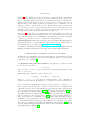
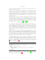
A-TINT: ALGORITHMIC TROPICAL INTERSECTION THEORY
7
Figure 1. The surface is X = max{1, x, y, z, −x, −y, −z} ⋅ R3 with
weights all equal to 1. The curve is max{3x+4, x−y−z, y+z +3}⋅X,
the weights are given by the labels.
polymake example: Computing a divisor.
This computes the divisors displayed in figure 1.
atint > $f = new MinMaxFunction(
INPUT STRING=>"max(1,x,y,z,-x,-y,-z)");
atint > $x = divisor(linear nspace(3),$f);
atint > $g = new MinMaxFunction(
INPUT STRING=>"max(3x+4,x-y-z,y+z+3)");
atint > $c = divisor($x,$g);
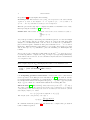
3.3. Irreducibility of tropical cycles. A property of classical varieties that one is
often interested in is irreducibility and a decomposition into irreducible components.
While one can easily define a concept of irreducible tropical cycles, there is in general
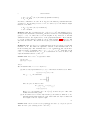
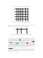
no unique decomposition (see Figure 2). We can, however, still ask whether a cycle
is irreducible and what the possible decompositions are.
Definition 3.10. We call a d-dimensional tropical cycle X irreducible if any other
d-dimensional cycle Y with ∣Y ∣ ⊆ ∣X∣ is an integer multiple of X.
Figure 2. The curve on the left is irreducible. The curve on the
right is reducible and there are several different ways to decompose
it.
To compute whether a cycle is irreducible, we have to introduce a few notations:
Definition 3.11. Let X be a tropical cycle with a fixed polyhedral structure X .
Let N be the number of maximal cells σ1 , . . . , σN of X . We identify an integer
vector ω ∈ ZN with the weight function σi ↦ ωi . We define
8
SIMON HAMPE
● ΛX ∶= {ω ∈ ZN ∶ (X , ω) is balanced} (which is a lattice).
● VX ∶= ΛX ⊗ R
Now fix a codimension one cell τ in X . Let S be the induced polyhedral structure
of StarX (τ ). For an integer vector ω ∈ Zn , we denote by ωS the induced weight
function on S. Then
● ΛτX ∶= {ω ∈ ZN ∶ (S, ωS ) is balanced}
● VXτ ∶= ΛτX ⊗ R
Remark 3.12. We obviously have ΛX = ⋂τ ∈X (dim X−1) ΛτX and similarly for VX .
Clearly, if X is irreducible, then dim VX should be 1 and vice versa (assuming that
gcd(ω1 , . . . , ωN ) = 1, where the ωi are the weights on X ). However, so far this
definition is tied to the explicit choice of the polyhedral structure. We would like
to get rid of this restriction, which we can do using Lemma 3.15. Hence we will
also write VX and ΛX . We call VX the weight space and ΛX the weight lattice of
X.
Definition 3.13. Let (X, ω) be a d-dimensional tropical cycle and X a polyhedral
structure on X. We define an equivalence relation on the maximal cells of X
in the following way: Two maximal cells σ, σ ′ are equivalent if and only if there
exists a sequence of maximal cells σ = σ0 , . . . , σr = σ ′ , σi ∈ X (d) such that for all
i = 0, . . . , r − 1, the intersection σi ∩ σi+1 is a codimension one cell of X , whose only
adjacent maximal cells are σi and σi+1 .
Lemma 3.14. Let σ and σ ′ be equivalent. Then:
(1) Vσ = Vσ′
(2) ω(σ) = ω(σ ′ )
Proof.
We can assume that σ ∩ σ ′ =∶ τ ∈ X (dim X−1) .
(1) Choose any representatives vσ/τ , vσ′ /τ of the lattice normal vectors. Then
ω(σ)vσ/τ + ω(σ ′ )vσ′ /τ ∈ Vτ
Let g1 , . . . , gr ∈ Λ∨ such that
⎛g1 ⎞
Vσ = ker ⎜ ⋮ ⎟
⎝gr ⎠
Since Vτ ⊆ Vσ , we have for all i:
0 = gi (ω(σ)vσ/τ + ω(σ ′ )vσ′ /τ ′ )
= ω(σ ′ )gi (vσ′ /τ ′ )
Hence vσ′ /τ ∈ Vσ and since Vσ′ = Vτ × ⟨vσ′ /τ ⟩, we have Vσ′ ⊆ Vσ . The other
inclusion follows analogously.
(2) X is balanced at τ if and only if StarX (τ ) is balanced, which is a onedimensional fan with exactly two rays. Such a fan can only be balanced if
the weights of the two rays are equal.
Lemma 3.15. Let X and X ′ be two polyhedral structures of a tropical cycle X.
Then VX ≅ VX ′ (and similarly for ΛX = VX ∩ ZN ).
A-TINT: ALGORITHMIC TROPICAL INTERSECTION THEORY
9
Proof. We can assume without loss of generality that X ′ is a refinement of X . Denote by N and N ′ the number of maximal cells of X and X ′ , respectively and fix
an order on the maximal cells of both structures. First of all, assume two maximal
cones of X ′ are contained in the same maximal cone of X . Since subdividing a
polyhedral cell produces equivalent cells in terms of definition 3.13, they must have
the same weight by Lemma 3.14. Thus the following map is well-defined: We partition {1, . . . , N ′ } into sets S1 , . . . , SN such that j ∈ Si ⇐⇒ σj′ ⊆ σi (where σj′ and
σi are maximal cells of X ′ and X , respectively). Pick representatives {j1 , . . . , jN }
from each partitioning set Si and let p ∶ VX ′ → RN be the projection on these coordinates jk . By the previous considerations, the map does not depend on the choice
of representatives. We claim that Im(p) ⊆ VX : Let τ be a codimension one cell of X
and τ ′ any codimension one cell of X ′ contained in τ . Then StarX (τ ) = StarX ′ (τ ′ ),
′
so if ω ∈ ZN makes X ′ balanced around τ ′ , then p(ω) makes X balanced around
τ . Bijectivity of p is obvious, so VX ≅ VX ′ .
Theorem 3.16. Let (X, ω) be a d-dimensional tropical cycle. Then X is irreducible
if and only if g ∶= gcd(ω(σ), σ ∈ X (d) ) = 1 and dim VX = 1.
Proof. Let X be irreducible. Clearly g must be 1, since otherwise a rational multiple
of X would provide a full-dimensional cycle in X not equal to k ⋅ X for an integer
k. Now assume dim VX = rank(ΛX ) > 1. Then we have an element ω ′ ∈ ZN that is
not a multiple of ω and such that (X, ω ′ ) is balanced, which is a contradiction to
our assumption that X is irreducible.
Now let g = 1 = dim VX . Assume X is not irreducible. Then we can find a polyhedral structure of X and two weight functions ω ′ , ω ′′ on this polyhedral structure
such that (X, ω ′ ), (X, ω ′′ ) are both balanced and ω ′ ≠ k ⋅ ω ′′ for any integer k. In
particular dim VX ≥ 2, which is a contradiction.
After having laid out these basics, we want to see how we can actually compute
this weight space:
Proposition 3.17. Let τ be a codimension one cell of a d-dimensional tropical
cycle X in Rn . Let u1 , . . . uk ∈ Zn be representatives of the normal vectors uσ/τ for
all σ > τ . Also, choose a lattice basis l1 , . . . , ld−1 of Λτ . We define the following
matrix:
Mτ ∶= (u1 . . . uk l1 . . . ld−1 ) ∈ Zn×(k+d−1)
Then ΛτX ≅ π(ker(Mτ ) ∩ Zk+d−1 ) × Z(N −k) , where π is the projection onto the first
k coordinates and N is again the number of maximal cells in X.
Proof. Fix an order on the maximal cells of X and let
J ∶= {j ∈ [N ] ∶ τ is not a face of σj }.
Then clearly Z(N −k) ≅ ⟨ej ; j ∈ J⟩Z ⊆ ΛτX and it is easy to see that ΛτX must be isomorphic to Z(N −k) ×ΛStarX (τ ) . Hence it suffices to show that ΛStarX (τ ) is isomorphic
to π(ker(Mτ ) ∩ Zk+d−1 ).
Let (a1 , . . . , ak , b1 , . . . , bl ) ∈ ker(Mτ ) ∩ Zk+d−1 , Then ∑ ai ui = ∑(−bi )li ∈ Λτ , so
StarX (τ ) is balanced if we assign weights ai . In particular (a1 , . . . , ak ) ∈ ΛStarX (τ ) .
Since l1 , . . . , ld−1 are a lattice basis, any choice of the ai such that StarX (τ ) is
balanced fixes the bi uniquely, so π is injective on ker(Mτ ) and surjective onto
ΛStarX (τ ) .
10
SIMON HAMPE
Algorithm 1 weightSpace(X)
1:
2:
Input: : A pure-dimensional polyhedral complex X
Output: : Its weight space VX
VX = RN
for τ a codimension one face of X do
Compute Mτ as above
VXτ = π(ker(Mτ )) + ⟨ej ∶ τ is not a face of σj ⟩
7:
VX = VX ∩ VXτ
8: end for
9: return VX
3:
4:
5:
6:
polymake example: Checking irreducibility.
This creates the six-valent curve from example 2 and computes its weight space (as
row vectors).
atint > $w = new WeightedComplex(
RAYS=>[[1,0],[1,1],[0,1],[-1,0],[-1,-1],[0,-1]],
MAXIMAL CONES=>[[0],[1],[2],[3],[4],[5]],
TROPICAL WEIGHTS=>[1,1,1,1,1,1]);
atint > print is irreducible($w);
# FALSE is displayed as an empty result
atint > print cycle weight space($w);
1 -1 1 0 0 0
0 0 1 0 0 1
1 0 0 1 0 0
0 1 0 0 1 0
This finally allows us to give an algorithm that computes VX :
Remark 3.18. One is often interested in the positive weights one can assign to a
complex X to make it balanced. This is now very easy using polymake: Simply
intersect VX with the positive orthant (R≥0 )N and you will obtain the weight cone
of X.
4. Intersection products in Rn
There are two main equivalent definitions for an intersection product in Rn , the
fan displacement rule [FS2, Theorem 3.2] and via rational functions [AR]. At first
sight, the computationally most feasible one seems to be the latter, since we can
already compute it with the means available to us so far:
Let X, Y be tropical cycles in Rn and ψi = max{xi , yi } ∶ Rn × Rn → R. Denote by
π ∶ Rn × Rn → Rn the projection onto the first n coordinates. Then we define
X ⋅ Y ∶= π∗ (ψ1 ⋅ ⋅ ⋅ ⋅ ⋅ ψn ⋅ (X × Y ))
(Here, applying π∗ just means forgetting the last n coordinates) However, computing this directly turns out to be rather inefficient. The main reason is that, since we
compute on the product X × Y , we multiply the number of their maximal cones by
each other and double the ambient dimension. As we have discussed earlier, both
are factors to which the computation of divisors reacts very sensitively.
A different definition of the intersection product is given by Jensen and Yu in [JY]:
A-TINT: ALGORITHMIC TROPICAL INTERSECTION THEORY
11
Theorem 4.1. Let X, Y be tropical cycles in Rn of dimension k and l respectively.
Let σ be a (k + l − n)-dimensional cone in the complex X ∩ Y and p any point in
rel int (σ). Then σ is a cell in X ⋅ Y if and only if the Minkowski sum
StarX (p) − StarY (p)
is complete, i.e. its support is Rn .
This definition is very close to the fan displacement rule and it is in fact not difficult
to see that they are equivalent. So, at first glance it would seem to be an unlikely
candidate for an efficient intersection algorithm. In particular, it is in general
algorithmically undecidable, whether a given fan is complete (see for example the
appendix of [N]). However, one can also show that StarX (p)−StarY (p) can be made
into a tropical fan (see [JY] for more details). Since Rn is irreducible, a tropical
fan is complete if and only if it is n-dimensional. In this case it is a multiple of Rn .
The weight of the cone σ in the above Theorem is then computed in the following
manner:
Lemma 4.2 ([JY]). Let σ be a polyhedral cell in X ⋅ Y . Let p ∈ rel int (σ). Then
ωX⋅Y (σ) =
∑
ρ1 ∈StarX (p),ρ2 ∈StarY (p)
s.t. p∈rel int (ρ1 −ρ2 )
ωX (ρ1 ) ⋅ ωY (ρ2 ) ⋅ ((Λρ1 + Λρ2 ) ∶ Λρ1 +ρ2 )
This now allows us to write down an algorithm based on these ideas:
Algorithm 2 MinkowskiIntersection
Input: Two tropical cycles X, Y in Rn of codimension k and l respectively,
such that k + l ≤ n
2: Output: Their intersection product X ⋅ Y
1:
3:
4:
5:
6:
7:
8:
9:
10:
11:
12:
13:
Compute the (n − (k + l))-skeleton Z of X ∩ Y
for σ a maximal cell in Z do
Compute an interior point p ∈ rel int σ
Compute the local fans StarX (p), StarY (p)
if for any ρ1 ∈ StarX (p), ρ2 ∈ StarY (p) the cell ρ1 − ρ2 is n-dimensional then
Compute weight ωX⋅Y of σ as described above
else
Remove σ
end if
end for
return (Z, ωX⋅Y )
polymake example: Computing an intersection product.
This computes the self-intersection of the standard tropical line in R2 .
atint > $l = tropical lnk(2,1);
atint > $i = intersect($l,$l);
atint > print $i->TROPICAL WEIGHTS;
1
12
SIMON HAMPE
5. Matroid fans
Matroid fans are an important object of study in tropical geometry, since they are
the basic building blocks of what we would consider as “smooth” varieties. There
are several different but equivalent ways of associating a tropical fan to a matroid,
see for example [AK, FR, FS1, S3, S]. One possibility, which immediately implies a
method to compute the fan, is given in [FS1, Proposition 2.5]:
Definition 5.1. Let M be a matroid on n elements. For w ∈ Rn let Mw be the
matroid whose bases are the bases σ of M of maximal w-cost ∑i∈σ wi . Then w lies
in the Bergman fan B(M ) if and only if Mw has no loops, i.e. the union of its bases
is the complete ground set.
Remark 5.2. The convex hull of the incidence vectors of the bases of a matroid is a
polytope in Rn , the so-called matroid polytope PM . So the vectors w maximizing a
certain basis are exactly the vectors in the normal cone of the vertex corresponding
to that basis. Hence the Bergman fan is a subfan of the normal fan of PM . In addition, we know that it has dimension rank(M ) (this follows immediately from other
possible definitions of B(M ), see for example [AK]). This gives us an algorithm to
compute B(M ):
Algorithm 3 bergmanFanFromNormalFan
1:
2:
Input: A matroid M on n elements, given in terms of its bases.
Output: Its Bergman fan in Rn
3:
4:
5:
Compute the normal fan F of the matroid polytope PM .
S = the rank(M )-skeleton of F .
for ξ a maximal cone in S do
Let ρ be the corresponding face of PM maximized by ξ
Let σ1 , . . . , σd be the bases corresponding to the vertices of ρ.
if ⋃ σi ⊊ [n] then
Remove ξ from S
end if
end for
return (S, ω ≡ 1)
6:
7:
8:
9:
10:
11:
12:
While this algorithm is fairly simple to implement, it is highly inefficient for two
reasons: Computing the skeleton of a fan from its maximal cones can be fairly
expensive, especially if we want to compute a low-dimensional skeleton. But mainly,
the problem is that from the potentially many cones of S we often only retain a
small fraction. Hence we compute a lot of superfluous information.
5.1. Computing matroid fans via circuits. A different definition of a matroid
fan can be given in terms of its circuits:
Definition 5.3. Let M be a matroid on n elements. Then B(M ) is the set of all
elements w ∈ Rn such that for all circuits C of M , the minimum min{wi ; i ∈ C} is
attained at least twice.
This definition actually produces the inversion in 0 of the fan in the first definition,
but that is obviously not a problem. It is used by Felipe Rincón in [R2] to compute
the Bergman fans of linear matroids, i.e. matroids associated to matrices. His algorithm requires the computation of a fundamental circuit C(e, I) for an independent
set I and some element e ∉ I such that I ∪ {e} is dependent:
C(e, I) = {e} ∪ {i ∈ I∣(I ∖ {i}) ∪ {e} is independent}
A-TINT: ALGORITHMIC TROPICAL INTERSECTION THEORY
13
It is an advantage of linear matroids that fundamental circuits can be computed
very efficiently purely in terms of linear algebra. For general matroids it can still
be computed using brute force. With this modified computation of fundamental
circuits the algorithm of Rincón can be used to compute Bergman fans of general
matroids. It turns out that this is still much faster than the normal fan algorithm
above. Table 4 in the appendix demonstrates this.
polymake example: Computing matroid fans.
This computes the Bergman fan of a matrix matroid and of the uniform matroid
U3,4 .
atint
atint
atint
atint
>
>
>
>
$m = new Matrix<Rational>([[1,-1,0,0],[0,0,1,-1]]);
$bm = Bergman fan linear($m);
$u = matroid::uniform matroid(3,4);
$bm2 = Bergman fan matroid($m);
5.2. Intersection products on matroid fans. Intersection products on matroid
fans have been studied in [S2],[FR]. Both approaches however are not suitable for
computation. While the approach in [S2] is more theoretical (except for surfaces,
where its approach might lead to a feasible algorithm), the description in [FR] might
seem applicable at first. The authors define rational functions which, applied to
B(M )×B(M ), cut out the diagonal. Hence they can define an intersection product
similar to [AR].
However, these rational functions are defined on a very fine polyhedral structure
of B(M ) induced by its chains of flats. These are very hard to compute ([KBE+ ]
gives an incremental polynomial time algorithm but [S1] states that already the
number of hyperplanes can be exponential) and the subdivision computed by the
algorithm of Rincón is in general much coarser. Also, recall that this approach to
computing an intersection product already proved to be inefficient in Rn .
It remains to be seen whether there might be a more suitable criterion for computation of matroid intersection products, maybe similar to Theorem 4.1.
6. Moduli spaces of rational curves
6.1. Basic notions. We only present the basic notations and definitions related
to tropical moduli spaces. For more detailed information, see for example [GKM].
Definition 6.1. An n-marked rational tropical curve is a metric graph with n
unbounded edges, labelled with numbers {1, . . . , n}, such that all vertices of the
graph are at least three-valent. We can associate to each such curve C its metric
n
vector (d(C)i,j )i<j ∈ R( 2 ) , where d(C)i,j is the distance between the unbounded
edges (called leaves) marked i and j determined by the metric on C.
n
Define Φn ∶ Rn → R( 2 ) , a ↦ (ai + aj )i<j . Then
n
Mn ∶= {d(C); C n-marked curve} ⊆ R( 2 ) /Φn (Rn )
is the moduli space of n-marked rational tropical curves.
Remark 6.2. It is shown (e.g. in [GKM]) that Mn is a pure (n−3)-dimensional fan
and if we assign weight 1 to each maximal cone, it is balanced (though they do not
use the standard lattice, as we will see below). Points in the interior of the same
cone correspond to curves with the same combinatorial type, i.e. forgetting their
metric, they are equal. In particular, maximal cones correspond to curves where
14
SIMON HAMPE
each vertex is exactly three-valent. We call this particular polyhedral structure on
Mn the combinatorial subdivision.
The lattice for Mn under the embedding defined above is generated by the rays
of the fan. These correspond to curves with exactly one bounded edge. Hence
each such curve defines a partition or split I∣I c on {1, . . . , n} and we denote the
resulting ray by vI (note that vI = vI c ). Given any rational n-marked curve, each
bounded edge Ei of length αi induces some split Ii , i = 1, . . . d on the leaves. In the
moduli space, this curve is then contained in the cone spanned by the vIi and can
be written as ∑ αi vIi .
While this description of Mn is very useful to understand the moduli space in terms
of combinatorics, it is not very suitable for computational purposes. By dividing
out Im(Φn ), we have to make some choice of projection, which would force us to do
a lot of tedious (and unnecessary) calculations. Also, the special choice of a lattice
would make normal vector computations difficult. However, there is a different
representation of Mn : It was proven in [AK] and [FR], that
Mn ≅ B(Kn−1 )/ ⟨(1, . . . , 1)⟩R
as a tropical variety, where Kn−1 is the matroid of the complete graph on n − 1
vertices. In paricular, matroid fans are always defined with respect to the standard
lattice. Dividing out the lineality space ⟨(1, . . . , 1)⟩ of a matroid fan can be done
without much difficulty, so we will usually want to represent Mn internally in matroid fan coordinates, while the user should still be able to access the combinatorial
information hidden within. The remaining parts of this section will be dedicated
to this purpose.
While the description of Mn as a matroid fan automatically gives us a way to
compute it, it turns out that this is rather inefficient. Furthermore, as soon as we
want to compute certain subsets of Mn , e.g. Psi-classes, the computations quickly
become infeasible due to the sheer size of the moduli spaces. Hence we would like
a method to compute Mn (or parts thereof) in some combinatorial manner. The
main instrument for this task is presented in the following subsection.
6.2. Prüfer sequences. Cayley’s Theorem states that the number of spanning
trees in the complete graph Kn on n vertices is nn−2 . One possible proof uses socalled Prüfer sequences: A Prüfer sequence of length n−2 is a sequence (a1 , . . . , an−2 )
with ai ∈ {1, . . . , n} (Repetitions allowed!). One can now give two very simple algorithms for converting a spanning tree in Kn into such a Prüfer sequence (Algorithm
4) and vice versa (Algorithm 5).
Algorithm 4 PrueferSequenceFromGraph(T)
1:
2:
3:
4:
5:
6:
7:
8:
Input: A spanning tree T in Kn
Output: A sequence P = (a1 , . . . , an−2 ), ai ∈ [n]
P ∶= ();
while No. of nodes of T > 2 do
Find the smallest node i that is a leaf and let v be the adjacent node
Remove i from T
P = (P, v)
end while
It is easy to see that this induces a bijection (see for example [AZ, Chapter 30]).
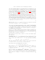
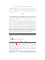
An example for this is given in Figure 3.
A-TINT: ALGORITHMIC TROPICAL INTERSECTION THEORY
15
Algorithm 5 GraphFromPrueferSequence(P)
1:
2:
3:
4:
5:
6:
7:
8:
9:
10:
11:
Input: A sequence P = (a1 , . . . , an−2 ), ai ∈ [n]
Output: A spanning tree T in Kn
T ∶= graph on n nodes with no edges
V ∶= [n]
while ∣V ∣ > 2 do
Let i ∶= min V ∖ P
Let j be the first element of P
Connect nodes i and j in T
Remove i from V and the first element from P
end while
Connect the two nodes left in V
1
2
5
3
6
(5,6,5,6)
4
Figure 3. An example for converting a spanning tree on K6 into
a Prüfer sequence and back. The tree can also be considered as
a 4-marked rational curve with additional labels at the interior
vertices.
As one can see from the picture, tropical rational n-marked curves with d bounded
edges can also be considered as graphs on n + d + 1 vertices: We convert the unbounded leaves into terminal vertices, labelled 1, . . . , n and arbitrarily attach labels
n + 1, . . . , n + d + 1 to the other vertices. This will allow us to establish a bijection between combinatorial types of rational curves and a certain kind of Prüfer
sequence:
Definition 6.3. A moduli Prüfer sequence of order n and length d is a sequence
(a1 , . . . , an+d−1 ) for some d ≥ 0, n ≥ 3 with ai ∈ {n + 1, . . . , n + d + 1} such that each
entry occurs at least twice.
We call such a sequence ordered if after removing all occurrences of an entry but
the first, the sequence is sorted ascendingly.
We denote the set of all sequences of order n and length d by Pn,d and the corre<
sponding ordered sequences by Pn,d
.
Example 6.4. The sequences (6, 7, 8, 7, 8, 6) and (6, 7, 6, 7, 8, 8) are ordered moduli
sequences of order 5 and length 2, but the sequence (6, 8, 8, 7, 7, 6) is not ordered.
Definition 6.5. For fixed n and d we call two sequences p, q ∈ Pn,d equivalent if
there exists a permutation σ ∈ S({n + 1, . . . , n + d + 1}) such that qi = σ(pi ) for all i.
<
Remark 6.6. It is easy to see that for fixed n and d the set Pn,d
forms a system of
representatives of Pn,d modulo equivalence, i.e. each sequence of order n and length
d is equivalent to a unique ordered sequence.
We will need this equivalence relation to solve the following problem: As stated
above, we want to associate Prüfer sequences to rational tropical curves by assigning
vertex labels n + 1, . . . , n + d + 1 to all interior vertices. There is no canonical way to
16
SIMON HAMPE
do this, so we can associate different sequences to the same curve. But two different
choices of labellings will then yield two equivalent sequences.
Proposition 6.7. The set of combinatorial types of n-marked rational tropical
<
curves is in bijection to ⋃n−3
d=0 Pn,d . More precisely, the set of all combinatorial
<
types of curves with d bounded edges is in bijection to Pn,d
.
Proof. The bijection is constructed as follows: Given an n-marked rational curve C
with d bounded edges, consider the unbounded leaves as vertices, labelled {1, . . . , n}.
Assign vertex labels {n + 1, . . . , n + d − 1} to the inner vertices. Then compute
the Prüfer sequence P (C) of this graph using Algorithm 4 and take the unique
equivalent ordered sequence as image of C.
First of all, we want to see that P (C) ∈ Pn,d . Since C has n+d+1 vertices if considered as above, the associated Prüfer sequence has indeed length n + d − 1. Furthermore, the n smallest vertex numbers are assigned to the leaves, so they will never
occur in the Prüfer sequence. Hence P (C) has only entries in {n + 1, . . . , n + d + 1}.
In addition, it is easy to see that each interior vertex v occurs exactly val(v) − 1
times (since we remove val(v) − 1 adjacent edges before the vertex becomes itself a
leaf), i.e. at least twice.
Injectivity follows from the fact that if two curves induce the same ordered sequence,
they can only differ by a relabelling of the interior vertices, so the combinatorial
types are in fact the same. Surjectivity is also clear, since the graph constructed
<
from any P ∈ Pn,d
is obviously a labelling of a rational n-marked curve.
We now present algorithm 6, which, given a moduli sequence, computes the corresponding combinatorial type in terms of its edge splits (it is more or less just a
slight modification of Algorithm 5):
Theorem 6.8. In the notation of Algorithm 6 the procedure generates the set of
splits I1 , . . . , Id of the combinatorial type corresponding to P . More precisely: If
v(i) is the element chosen from V in iteration i ∈ {n + 1, . . . , n + d − 1}, then In−i is
the split on the leaves {1, . . . , n} induced by the edge {v(i), pi }.
Proof. Let v(i) be the element chosen in iteration i, corresponding to vertex wi in
the curve. In particular i ∉ P . This means that i has already occurred val(wi ) − 1
times in the sequence P as P [0]. Hence the node v(i) is already (val(wi ) − 1)valent, i.e. connected to nodes qj ; j = 1, . . . , val(wi ) − 1. If qj is a leaf (i.e. ≤ n), then
qj ∈ Av(i) . Otherwise, qj must have been chosen as v(k) in a previous iteration
k < i. Hence it must already be val(wk )-valent. Inductively we see that each node
“behind” qj is either a leaf or has already full valence. In particular, no further
edges will be attached to any of these nodes.
By induction on i, the edge {v(i), qj } (assuming qj is not a leaf) corresponds to the
split Aqj . In particular, Aqj has been added to Av . Hence Av is the split induced
by the edge {v(i), pi }.
<
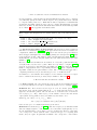
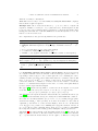
Example 6.9. Let us apply algorithm 6 to the following sequence P ∈ P8,5
(see
figure 4 for a picture of the corresponding curve):
P = (9, 9, 10, 10, 11, 11, 12, 12, 13, 13, 14, 14).
The algorithm begins by attaching the leaves {1, . . . , 8} to the appropriate vertices,
i.e. after the first for-loop we have A9 = {1, 2}, A10 = {3, 4}, A11 = {5, 6}, A12 = {7, 8}
and P = (13, 13, 14, 14), V = {9, . . . , 14}. Now the minimal element of V ∖ P is v = 9.
We set I1 = A9 = {1, 2} to be the split of the first edge. Then we connect the vertex 9
A-TINT: ALGORITHMIC TROPICAL INTERSECTION THEORY
17
Algorithm 6 combinatorialTypeFromPrueferSequence(P ,n)
1:
2:
Input: A moduli sequence P = (p1 , . . . , pN ) ∈ Pn,d
Output: The rational tropical n-marked curve associated to P in terms of the
splits I1 , . . . , Id induced by its bounded edges.
3:
4:
5:
d=N −n+1
V = {1, . . . , n + d + 1}
An+1 , . . . , An+d+1 = ∅
//First: Connect leaves
for i = 1 . . . n do
Api = Api ∪ {i}
V = V ∖ {i}
P = (pi+1 , . . . , pN )
end for
//Now create edges
for i = n + 1 . . . n + d − 1 do
v = min V ∖ P
Ii−n = Av
if length(P ) > 0 then
//We denote by P [0] the first element of the sequence P .
AP [0] = AP [0] ∪ Av
V = V ∖ {i}
P = (pi+1 , . . . , pN )
end if
end for
//Create final edge
Id = Amin V
6:
7:
8:
9:
10:
11:
12:
13:
14:
15:
16:
17:
18:
19:
20:
21:
22:
23:
24:
to the first vertex in P , which is 13. Hence A13 = A13 ∪A9 = {1, 2}. We remove 9 from
V and set P to be (13, 14, 14). Now v = min V ∖ P = 10. We obtain the second split
I2 = A10 = {3, 4}. The we connect vertex 10 to 13, so A13 = A13 ∪ A10 = {1, 2, 3, 4}.
We set V = {11, 12, 13, 14} and P = (14, 14). In the next two iterations we obtain
splits I3 = A11 = {5, 6}, I4 = A12 = {7, 8} and we connect both 11 and 12 to 14,
setting A14 = {5, 6, 7, 8}. Now P = () and V = {13, 14}, so we leave the for-loop and
set the final split to be I5 = A13 = {1, 2, 3, 4}.
3
1
2
9
4 5
6
10
11
13
14
7
12
8
Figure 4. The curve corresponding to the moduli sequence P ,
including labels for the interior vertices.
6.3. Enumerating maximal cones of Mn . We now want to apply the results of
the previous section to compute Mn . For this it is of course sufficient to compute
all maximal cones. More precisely, we will only need to compute all combinatorial
types corresponding to maximal cones, i.e. rational n-marked tropical curves whose
vertices are all three-valent. Using Algorithm 6 we can then compute its rays
vI1 , . . . , vIn−3 . These can easily be converted into matroid coordinates with the
construction given in [FR, Example 7.2].
18
SIMON HAMPE
Proposition 6.7 directly implies the following:
Corollary 6.10. The maximal cones of Mn are in bijection to all ordered Prüfer
sequences of order n and length n − 3, i.e. sequences (a1 , . . . , a2n−4 ) with ai in
{n + 1, . . . , 2n − 2} such that each entry occurs exactly twice.
This also gives us an easy way to compute the number of maximal cones of Mn ,
thus reproving the formula of [SS, Theorem 3.4]:
Lemma 6.11. The number of maximal cones in the coarse subdivision of Mn is
n−4
∏ (2(n − i) − 5)
i=0
Proof. We prove this by constructing ordered Prüfer sequences of order n and length
n − 3. The sequence has 2n − 4 entries. Since it is ordered, the first entry must
always be n + 1. This entry must occur once more, so we have 2n − 5 possibilities to
place it in the sequence. Assume we have placed all entries n + 1, . . . , n + k, each of
them twice. Then the first free entry must be n+k +1, since the sequence is ordered
and we have 2(n − k) − 5 possibilities to place the remaining one. This implies the
formula.
As one can see, the complexity of this number is in O(nn−3 ), so there is no hope
for a fast algorithm to compute all of Mn for larger n (except using symmetries).
As we will see later, however, we are sometimes only interested in certain subsets
or local parts of Mn .
polymake example: Computing Mn .
This computes tropical M0,8 and displays the number of its maximal cones.
atint > $m = tropical m0n(8);
atint > print $m->MAXIMAL CONES->rows();
10395
6.4. Computing products of Psi-classes. A factor that often occurs in intersection products on moduli spaces are Psi-classes. In [KM], the authors describe
tropical Psi-classes as (multiples of) certain divisors of rational functions, but also
in combinatorial terms. For nonnegative integers k1 , . . . , kn and I ⊆ [n], they define
K(I) ∶= ∑i∈I ki . Then one of their main results is the following Theorem
Theorem 6.12 ([KM, Theorem 4.1]). The intersection product ψ1k1 ⋅⋅ ⋅ ⋅⋅ψnkn ⋅Mn is
the subfan of Mn consisting of the closure of the cones of dimension n − 3 − K([n])
corresponding to the abstract tropical curves C such that for each vertex V of C we
have val(V ) = K(IV ) + 3, where
IV = {i ∈ [n] ∶ leaf i is adjacent to V } ⊆ [n].
The weight of the corresponding cone σ(C) is
ω(σ(C)) =
∏V ∈V (C) K(IV )!
.
n
∏i=1 ki !
In combination with Proposition 6.7, this allows us to compute these products in
terms of Prüfer sequences:
A-TINT: ALGORITHMIC TROPICAL INTERSECTION THEORY
19
Corollary 6.13. The maximal cones in ψ1k1 ⋅ ⋅ ⋅ ⋅ ⋅ ψnkn ⋅ Mn are in bijection to the
<
ordered moduli sequences P ∈ Pn,n−3−K([n])
that fulfill the following condition:
Let d = n − 3 − K([n]) and ki = 0 for i = n + 1, . . . , n + d − 1. For any a ∈
{n + 1, . . . , n + d + 1} let j1 , . . . , jl(a) ∈ {1, . . . , n + d − 1} be the indices such that
Pji = a. Then
l(a)
l(a) = 2 + ∑ kjl
l=1
Proof. Recall that any entry a corresponding to a vertex va in the curve C(P )
occurs exactly val(va ) − 1 times. By the Theorem above the valence of a vertex is
dictated by the leaves adjacent to it. Furthermore, the leaves adjacent to a vertex
va can be read off of the first n entries of the sequence: Leaf i is adjacent to va if
and only if Pi = a.
So, given a curve in the Psi-class product, vertex va must have valence 3 + K(Iva ),
so it occurs 2 + K(Iva ) = 2 + ∑i∶Pi =a ki times. Conversely, given a sequence fulfilling
the above condition, we obviously obtain a curve with the required valences.
We now want to give an algorithm that computes all of these Prüfer sequences.
As it turns out, this is easier if we require the ki to be in decreasing order, i.e.
k1 ≥ k2 ≥ ⋅ ⋅ ⋅ ≥ kn . In the general case we will then have to apply a permutation to
the ki before computation and to the result afterwards. The general idea is that we
recursively compute all possible placements of each vertex that fulfill the conditions
imposed by the ki (if we place vertex a at leaf i with ki > 0, then it has to occur
more often). Due to its length, the algorithm has been split into several parts:
iteratePlacements goes through all possible entries of the Prüfer sequence recursively. It uses placements to compute all possible valid distributions of an
entry, given a certain configuration of free spaces in the Prüfer sequence.
Algorithm 7 psiProductSequencesOrdered(k1 , . . . , kn )
1:
2:
Input: Nonnegative integers k1 ≥ k2 ≥ ⋅ ⋅ ⋅ ≥ kn
Output: All Prüfer sequences corresponding to maximal cones in ψ1k1 ⋅ ⋅ ⋅ ⋅ ⋅ ψnkn ⋅
Mn
K = ∑ ki
current vertex = n + 1
current sequence = (0, . . . , 0) ∈ Z2n−4−K
6: exponents = (k1 , . . . , kn , 0, . . . , 0) ∈ Z2n−4−K
3:
4:
5:
7:
iteratePlacements(current vertex, current sequence)
Proof. (of Algorithm 7) First of all we prove that placements computes indeed all
possible subsets J ∈ [m] such that ∣J∣ = 2 + ∑j∈J kj . So let J = {a1 , . . . , aN } be such
a set with a1 ≤ ⋅ ⋅ ⋅ ≤ aN . It is easy to see that in each iteration of the while-loop we
have ∣J∣ = i − 1. Let δ = (2 + ∑j∈J kj ) − ∣J∣.
One can see by induction on δ that, starting in any iteration of the while loop,
the algorithm will eventually reach an iteration where i is one smaller. This proves
termination of placements.
But we can only reach the iteration where i = 0 if in the previous iteration we have
tried all indices {1, . . . , m} as first element of J. In particular, there was a previous
iteration, where we chose l = a1 as first element of J. Now assume we are in the
first iteration where J = {a1 , . . . , as }, 1 ≤ s < N . Assuming δ > 0, we can again only
20
SIMON HAMPE
iteratePlacements(current vertex, current sequence)
1:
2:
3:
4:
5:
6:
7:
8:
9:
10:
11:
12:
if current vertex > 2n − 2 − K then
if current sequence contains no 0’s then
append current sequence to result
end if
else
f = {i ∶ current sequence[i] = 0}
for P ∈ placements((exp[i], i ∈ f )) do
v = current sequence
Place current vertex in v at positions indicated by P
iteratePlacements(current vertex+1,v)
end for
end if
placements(k1 , . . . , km )
1:
2:
Input: Positive integers k1 ≥ ⋅ ⋅ ⋅ ≥ km
Output: All subsets J ⊆ [m] such that ∣J∣ = 2 + ∑j∈J kj .
3:
4:
5:
Let J = ∅, i = 1
while i > 0 do
if ∣J∣ < 2 + ∑j∈J kj then
Let l ∈ [m] ∖ J be minimal such that l > max J and we haven’t used it yet
as i-th element of J.
if There is no such l then
stepDown
else
Add l to the indices we have used as i-th element of J
i=i+1
J = J ∪ {l}
end if
else
Add J to solution
stepDown
end if
end while
6:
7:
8:
9:
10:
11:
12:
13:
14:
15:
16:
17:
18:
stepDown
1: Forget all indices we used as i-th element of J.
2: J = J ∖ {max(J)}
3: i = i − 1
decrease i if we have tried all valid placements, including as+1 . So assume δ = 0.
Then {a1 , . . . , as } is a valid placement, i.e. s = 2 + ∑si=1 kai . If we subtract this from
the equation for J, we obtain
N
0 < N − s = ∑ kai
i=s+1
In particular, since the ki are ordered, we must have kas+1 ≥ 1 and hence also kaj ≥ 1
for all j ≤ s. This implies
s
s = 2 + ∑ kai ≥ 2 + s
i=1
A-TINT: ALGORITHMIC TROPICAL INTERSECTION THEORY
21
which is obviously a contradiction.
With this it is now easy to see that psiProductSequencesOrdered computes
indeed all the required sequences.
Example 6.14. We do indeed need that k1 ≥ ⋅ ⋅ ⋅ ≥ kn to be able to compute all
sequences. Assume n = 7 and (k1 . . . k7 ) = (0, 0, 0, 0, 0, 1, 1). A valid sequence would
be (7, 7, 8, 8, 9, 7, 7, 9), but this sequence would never occur in the algorithm: After
having placed the first two 7’s in placements we would already have δ = 0, so the
last two 7’s are never tried out.
For completeness we also give the algorithm for the general case:
Algorithm 8 psiProductSequences(k1 , . . . , kn )
2:
Input: A list of nonnegative integers k = k1 , . . . , kn
Output: All Prüfer sequences corresponding to maximal cones in ψ1k1 ⋅ ⋅ ⋅ ⋅ ⋅ ψnkn ⋅
Mn
3:
4:
5:
Let σ ∈ Sn such that σ(k) is ordered descendingly
l = psiProductSequencesOrdered(σ(k))
return σ −1 (l) (applied elementwise to the first n entries of each sequence)
1:
polymake example: Computing psi classes.
This computes ψ13 ⋅ ψ22 ⋅ ψ6 ⋅ M0,9 (which is a point) and displays its multiplicity.
atint > $p = psi product(9, new Vector<Int>(3,2,0,0,0,1,0,0,0));
atint > print $p->TROPICAL WEIGHTS;
60
6.5. Computing rational curves from a given metric. In previous sections
we computed rational curves as elements of the moduli space given by their corresponding bounded edges, i.e. the vI that span the cone containing the curve.
Usually, we will be given the curves either in the matroid coordinates of the moduli
n
space or as a vector in R( 2 ) , i.e. a metric on the leaves. It is relatively easy to
convert the matroid coordinates to a metric, but it is not trivial to convert the
metric to a combinatorial description of the curve, i.e. a list of the splits induced
by the bounded edges and their lengths.
The paper [B] describes an algorithm to obtain a tree from a metric d on a given
set S that fulfills the four-point-condition, i.e. for all x, y, z, t ∈ [n] we have
d(x, y) + d(z, t) ≤ max{d(x, z) + d(y, t), d(x, t) + d(y, z)}
and [BG, Theorem 2.1] shows that the metrics induced by semi-labelled trees (essentially: rational n-marked curves) are exactly those which fulfill this condition.
Note that we can always assume d(x, y) > 0 for x ≠ y by adding an appropriate
n
element from Im(Φn ). More precisely, if we have an element d ∈ R( 2 ) that is
equivalent to the metric of a curve modulo Im(Φn ), there is a k ∈ N such that
d + k ⋅ Φn (∑ ei ) is a positive vector fulfilling the four-point-condition. In fact, if
m = d + ∑ αi Φn (ei ) is the equivalent metric, then d + ∑(αi + ∣αi ∣)Φn (ei ) still fulfills
the four-point-condition, since adding positive multiples of Φn (ei ) preserves it.
Algorithm 9 gives a short sketch of the algorithm described in [B, Theorem 2]. As
input, we provide a metric d. We then obtain a metric tree with leaves L labelled
{1, . . . , n} such that the metric induced on L is equal to d. This tree corresponds
22
SIMON HAMPE
to a rational n-marked curve: Just replace the bounded edges attached to the leaf
vertices by unbounded edges. It is very easy to modify the algorithm such that it
also computes the splits of all edges.
Algorithm 9 treeFromMetric(d) [B, Theorem 2]
1:
2:
Input: A metric d on the set [n] fulfilling the four-point-condition.
Output: A metric tree T with leaf vertices L labelled {1, . . . , n} such that the
induced metric on L equals d.
Let V = {1, . . . , n}
while ∣V ∣ > 3 do
5:
Find ordered triple of distinct elements (p, q, r) from V , such that
d(p, r) + d(q, r) − d(p, q) is maximal
6:
Let t be a new vertex and define its distance to the other vertices by
1
d(t, p) = (d(p, q) − d(p, r) − d(q, r))
2
d(t, x) = d(x, p) − d(t, p) for x ≠ p
3:
4:
7:
8:
9:
10:
If d(t, x) = 0 for any x, identify t and x, otherwise add t to V .
Attach p and q to t. Then remove p and q from V
end while
Compute the tree on the remaining vertices using linear algebra.
polymake example: Converting curve descriptions.
This takes a ray from M0,6 (in its moduli coordinates) and displays it in different
representations.
atint > $m = tropical m0n(6);
atint > $r = $m->RAYS->row(0);
atint > print $r;
-1 -1 -1 0 -1 -1 0 -1 0
atint > $c = rational curve from moduli($r);
atint > print $c;
(1,2,3,4)
# This means that this ray represents v{1,2,3,4}
atint > print $c->metric vector;
0 0 0 1 1 0 0 1 1 0 1 1 1 1 0 # Read as d(1, 2), d(1, 3), . . . , d(5, 6)
6.6. Local bases of Mn . When computing divisors or intersection products on
moduli spaces Mn , a major problem is the sheer size of the fans, in the number
of cones and in the dimension of the ambient space. The number of cones can
usually be reduced to an acceptable amount, since one often knows that only a
handful of cells is actually relevant. However, the ambient dimension of Mn is
2
(n2 )−n = n −3n
∈ O(n2 ). Convex hull computations and operations in linear algebra
2
thus quickly become expensive. We will show, however, that locally at any point
0 ≠ p ∈ Mn , the span of StarMn (p) has a much lower dimension. Hence we can do
all our computations locally, where we embed parts of Mn in a lower-dimensional
space. Let us make this precise:
Definition 6.15. Let τ be a d-dimensional cone of Mn . We define
V (τ ) ∶= ⟨{σ ≥ τ ; σ ∈ Mn }⟩R = ⟨U (τ )⟩R ,
where U (τ ) = ⋃σ≥τ rel int (σ). It is easy to see that for any 0 ≠ p ∈ Mn and τ the
minimal cone containing p, the span of StarMn (p) is exactly V (τ ).
A-TINT: ALGORITHMIC TROPICAL INTERSECTION THEORY
23
We are now interested in finding a basis for this space V (τ ), preferably without
having to do any computations in linear algebra. The idea for this is the following:
Let Cτ be the combinatorial type of an abstract curve represented by an interior
point of τ . We want to find a set of rays vI , all contained in some σ ≥ τ , that
generate V (τ ). Each such ray corresponds to separating edges and leaves at a
vertex p of Cτ along a new bounded edge (whose split is of course I∣I c ). We will
see that for a fixed vertex p with valence greater than 3, all the rays separating
that vertex span a space that has the same ambient dimension as Mval(p) . In fact,
it is easy to see that they must be in bijection to the rays of that moduli space.
Hence the idea for constructing a basis is the following: In addition to the rays
of τ , we choose a basis for the “Mval(p) ” at each higher-valent vertex p. This
choice is similar to the one in [KM, Lemma 2.3]. There the authors show that
Vk ∶= {vS , ∣S∣ = 2, k ∉ S} is a generating set of the ambient space of Mn for any
k ∈ [n] and it is easy to see that by removing any element it becomes a basis.
Now fix a vertex p of Cτ such that s ∶= val(p) > 3. Denote by I1 , . . . , Is the splits
on [n] induced by the edges and leaves adjacent to p (in particular, some of the Ij
might only contain one element). We now define
Wp ∶= {vIi ∪Ij ; i, j ≠ 1, i ≠ j}
(This corresponds to the set V1 described above) and
Bp ∶= Wp ∖ {vI2 ∪I3 }.
Clearly all the following results also hold if we choose i, j ≠ k for some k > 1
or remove a different element in the definition of Bp (in particular, because the
numbering of the Ii is completely arbitrary). To make the proofs more concise, we
will however stick to this particular choice. We introduce one final notation: For
∣Ij ∣ = 1, we set vIj ∶= 0.
Lemma 6.16 (see also [KM, Lemmas 2.4 and 2.7]).
(1) Let p be a vertex of the generic curve Cτ and define I1 , . . . , Is , Wp as above.
Then
⎛
⎞
∑ v = (s − 3) ∑ vIj + vI1 ≡ 0 mod Vτ .
⎝j>1 ⎠
v∈Wp
(2) Let vI be a ray in some σ ≥ τ and assume it separates some vertex p of Cτ .
Define I1 , . . . , Is , Wp as above. Assume without restriction that I1 ⊆ I c .
Then
vI = ∑ vS − (m − 2)( ∑ vIj + vI ) ≡ ∑ vS mod Vτ .
vS ∈Wp
S⊆I
Ij ⊆I
vS ∈Wp
S⊆I
Proof.
(1) We define a = (ai ) ∈ Rn via ai = 1, if i ∈ I1 and ai = (s − 3) otherwise.
Furthermore we define b = (bi ) ∈ Rn via
⎧
0,
if i is a leaf attached to p
⎪
⎪
⎪
⎪
bi = ⎨1,
if i is not a leaf at p and lies in I1
⎪
⎪
⎪
⎪
(s
−
3),
if i is not a leaf at p and does not lie in I1 .
⎩
24
SIMON HAMPE
We now prove the following equation (to be considered as an equation in
n
R( 2 ) , where each ray is represented by its metric vector):
⎛
⎞
⎜
⎟
+ v − φn (b) + φn (a).
∑ v = (s − 3) ⎜
∑ vIj ⎟
⎜
⎟ I1
j>1
v∈Wp
⎝∣Ij ∣>1 ⎠
n
We index R( 2 ) by all sets T = {k1 , k2 }, k1 ≠ k2 . We have
⎧
0,
if k1 , k2 ∈ Ij , j = 1, . . . , s
⎪
⎪
⎪
⎛
⎞
⎪
= ⎨s − 2,
if k1 ∈ I1 , k2 ∈ Ij , j > 1
∑ v
⎪
⎝v∈Wp ⎠
⎪
⎪
T
⎪
⎩2(s − 3), if k1 ∈ Ii , k2 ∈ Ij ; i, j > 1; i ≠ j.
We now study the right hand side in four different cases:
(a) If k1 , k2 ∈ I1 , then both are not leaves at p. Hence the right hand side
yields 0 + 0 − 2 + 2 = 0.
(b) If k1 , k2 ∈ Ij , j > 1, again both are not leaves at p. The right hand side
now yields 0 + 0 − 2(s − 3) + 2(s − 3) = 0.
(c) Assume k1 ∈ Ii , k2 ∈ Ij , i, j > 1 and i ≠ j. If both are not leaves at
p, we get 2(s − 3) + 0 − 2(s − 3) + 2(s − 3). If only one is a leaf, we
get (s − 3) + 0 − (s − 3) + 2(s − 3). Finally, if both are leaves, we get
0 + 0 − 0 + 2(s − 3). So in any of these cases the right hand side agrees
with the left hand side.
(d) Assume k1 ∈ I1 , k2 ∈ Ij , j > 1. If both are not leaves, we get (s − 3) +
1 − (s − 3) − 1 + (s − 2). The other cases are similar.
(2) We know that I must be a union of some of the Ij and we assume without
restriction that I = ⋃j≥k Ij for some k > 1. Furthermore we define
m ∶= ∣{i ∶ Ii ⊆ I}∣ = s − k + 1.
n
We now prove the following formula (again in R( 2 ) . A similar formula for
the representation of a ray vI in Vk and a similar proof can be found in
[KM, Lemma 2.7]):
vI = ∑ vIi ∪Ij − (m − 2)φn (∑ el )
l∈I
i,j≥k
´¹¹ ¹ ¹ ¹ ¹ ¹ ¹ ¹ ¹ ¹ ¹ ¹ ¹ ¹ ¹ ¹ ¹ ¹ ¹ ¹ ¹ ¹ ¹ ¹ ¹ ¹ ¹ ¹ ¹ ¹ ¹ ¹ ¹ ¹ ¹ ¹ ¹ ¹ ¹ ¹ ¹ ¹ ¹ ¹ ¹ ¹ ¹ ¹ ¹ ¸¹ ¹ ¹ ¹ ¹ ¹ ¹ ¹ ¹ ¹ ¹ ¹ ¹ ¹ ¹ ¹ ¹ ¹ ¹ ¹ ¹ ¹ ¹ ¹ ¹ ¹ ¹ ¹ ¹ ¹ ¹ ¹ ¹ ¹ ¹ ¹ ¹ ¹ ¹ ¹ ¹ ¹ ¹ ¹ ¹ ¹ ¹ ¹ ¹ ¶
=∶z
n
⎛
⎞
− (m − 2) ∑ vIj + vI − φn (∑ ei )
⎝j≥k
⎠
i=1
´¹¹ ¹ ¹ ¹ ¹ ¹ ¹ ¹ ¹ ¹ ¹ ¹ ¹ ¹ ¹ ¹ ¹ ¹ ¹ ¹ ¹ ¹ ¹ ¹ ¹ ¹ ¹ ¹ ¹ ¹ ¹ ¹ ¹ ¹ ¹ ¹ ¹ ¹ ¹ ¹ ¹ ¸ ¹ ¹ ¹ ¹ ¹ ¹ ¹ ¹ ¹ ¹ ¹ ¹ ¹ ¹ ¹ ¹ ¹ ¹ ¹ ¹ ¹ ¹ ¹ ¹ ¹ ¹ ¹ ¹ ¹ ¹ ¹ ¹ ¹ ¹ ¹ ¹ ¹ ¹ ¹ ¹ ¹ ¶
=∶w
≡ ∑ vIi ∪Ij mod Vτ .
(6.1)
i,j≥k
n
To see that the equation holds, let us first compute w. We index R( 2 ) by
all sets T ∶= {k1 , k2 }, k1 ≠ k2 . Then we have
⎧
0, if {k1 , k2 } ⊆ Ii for some i ≥ k
⎪
⎪
⎪
⎪
= ⎨1, if k1 ∈ I, k2 ∉ I or vice versa
⎪
⎪
⎪
{k1 ,k2 }
⎪
⎩2, if k1 ∈ Ii , k2 ∈ Ij , i ≠ j; i, j ≥ k.
⎛
⎞
∑ vI
⎝j≥k j ⎠
A-TINT: ALGORITHMIC TROPICAL INTERSECTION THEORY
25
Hence
⎧
0,
⎪
⎪
⎪
⎪
= ⎨2,
⎪
⎪
⎪
{k1 ,k2 }
⎪
⎩2,
⎧
⎪0,
⎪
=⎨
⎪
2,
⎪
⎩
⎛
⎞
∑ vIj + vI
⎝j≥k
⎠
if {k1 , k2 } ⊆ Ii for some i ≥ k
if k1 ∈ I, k2 ∉ I or vice versa
if k1 ∈ Ii , k2 ∈ Ij , i ≠ j; i, j ≥ k
if {k1 , k2 } ⊆ Ii for some i ≥ k
otherwise.
Finally we get
⎧
⎪
⎪−2, if {k1 , k2 } ⊆ Ii for some i ≥ k
(w){k1 ,k2 } = ⎨
⎪
0, otherwise.
⎪
⎩
Thus it remains to prove that
⎧
⎪
⎪2(m − 2), if {k1 , k2 } ⊆ Ii for some i ≥ k
(vI − z){k1 ,k2 } = ⎨
⎪
0, otherwise.
⎪
⎩
For this, let k1 ≠ k2 ∈ [n]. If T ∶= {k1 , k2 } ⊆ Ii for some i ≥ k, then
(vI )T = (vIi ∪Ij )T = 0 for all i, j ≥ k and (φn (∑l∈I el ))T = 2. Thus the
formula holds. Now if k1 ∈ Ii , k2 ∈ Ij for i ≠ j and i, j ≥ k, we still have
(vI )T = 0. Furthermore, there are (m−2) choices for a ray vIi ∪Ij′ with j ′ ≠ j
and (m − 2) choices for a ray vIi′ ∪Ij with i′ ≠ i. For these rays, the T -th
entry is 1, for all other rays vIi′ ∪Ij′ it is 0. Hence
⎛
⎞
= 2(m − 2) = (m − 2) (φn (∑ el )) .
∑ vIi ∪Ij
⎝i,j≥k
⎠
l∈I
T
T
Finally, if k1 ∈ I (say k1 ∈ Ii ), k2 ∉ I, then (vI )T = 1. There are (m − 1)
choices for a ray vIi ,Ij with j ≠ i. Since (φn (∑l∈I el ))T = 1, we get
⎛
⎞
= (m − 1) = (m − 2) (φn (∑ el )) + 1.
∑ vIi ∪Ij
⎝i,j≥k
⎠
l∈I
T
T
Hence equation 6.1 holds.
Theorem 6.17. Let vE1 , . . . , vEt be the rays of τ . Then the set
Bτ ∶=
Bp ∪ {vE1 , . . . , vEt }
⋃
p∈Cτ(0)
val(p)>3
is a basis for V (τ ). In particular, the dimension of V (τ ) can be calculated as
dim V (τ ) = dim τ +
∑
p∈Cτ(0)
val(p)>3
((
val(p)
) − val(p)) .
2
Proof. By Lemma 6.16 these rays generate Vτ : We can write each vI in some σ ≥ τ
in terms of Wp and the bounded edges at the vertex associated to it. The first
part of the Lemma then yields that we can replace any occurrence of vI2 ∪I3 to get
a representation in Bp and the bounded edges.
To see that the set is linearly independent, we do an induction on n. For n = 4 the
statement is trivial. For n > 4, assume τ is the vertex of Mn . Then Bτ actually
agrees with the set Vk ∖ {vS } for some S and we are done. So let p be a vertex
of Cτ that has only one bounded edge attached and denote by i one of the leaves
26
SIMON HAMPE
attached to it. It is easy to see that applying the forgetful map fti to Bτ , we get
the set Bfti (τ ) . If p is three-valent, then the ray corresponding to the bounded edge
at p is mapped to 0 and all other elements of Bτ are mapped bijectively onto the
elements of Bfti (τ ) . Since the latter is independent by induction, so is Bτ .
If p is higher-valent, only rays from Bp might be mapped to 0 or to the same
element. Hence, if we have a linear relation on the rays in Bτ , we can assume by
induction that only the elements in Bp have non-trivial coefficients. But these are
linearly independent as well: Let q be any other vertex with only one bounded edge
and j any leaf at q. Bp is now preserved under the forgetful map ftj and hence
linearly independent by induction.
At the beginning of this section we introduced the notion that the rays resolving a
certain vertex of a combinatorial type Cτ “look like Mval(p) ”. The results above
allow us to make this notion precise:
Corollary 6.18. Let M be any polyhedral structure of Mn (and hence a refinement
of the combinatorial subdivision). Let τ ∈ M be a d-dimensional cell. Let Cτ be the
combinatorial type of a curve represented by a point in the relative interior of τ .
Denote by p1 , . . . , pk its vertices and by l the number of bounded edges of the curve.
Then
StarMn (τ ) ≅ Rl−d × Mval(p1 ) × ⋅ ⋅ ⋅ × Mval(pk )
Proof. First assume M is the combinatorial subdivision of Mn . There is an obvious
map
ψτ ∶ StarMn (τ ) → Mval(p1 ) × ⋅ ⋅ ⋅ × Mval(pk ) ,
defined in the following way: For each vertex pi of Cτ fix a numbering of the
adjacent edges and leaves, I1 , . . . , Iji . Now for each vI in some σ ≥ τ , there is
a unique i ∈ {1, . . . , k} such that vI separates pi . Let S ⊆ {1, . . . , ji } such that
I = ⋃j∈S Ij . Again, this choice is unique. Now map vI to vS in Mval(pi ) . It is easy
to see that this map must be bijective.
First let us see that the map is linear. By Theorem 6.17 we only have to check
that the map respects the relations given in Lemma 6.16. But this is clear, since
analogous equations hold in Mn (again, see [KM, Lemmas 2.4 and 2.7] for details).
For any set of rays vJ1 , . . . , vJk associated to the same vertex of Cτ it is easy to see
that they span a cone in Mn if and only if their images do. Now if σ ≥ τ is any cone,
we can partition its rays into subsets Sj , j = 1, . . . , m that are associated to the same
vertex pj . Each of these sets of rays span a cone σj which is mapped to a cone in
Mval(pj ) . Since σ = σ1 × ⋅ ⋅ ⋅ × σm , it is mapped to a cone in Mval(p1 ) × ⋅ ⋅ ⋅ × Mval(pm ) .
Hence ψτ is an isomorphism.
Finally, if M is any polyhedral structure, let τ ′ be the minimal cone of the combinatorial subdivision containing τ . Then l = dim τ ′ and we have
StarMn (τ ) ≅ Rl−d × StarMn (τ ′ )
A-TINT: ALGORITHMIC TROPICAL INTERSECTION THEORY
27
polymake example: Local computations in Mn .
This computes a local version of M0,13 around a codimension 2 curve C with a
single five-valent vertex, i.e. it computes all maximal cones containing the cone
corresponding to C. a-tint keeps track of the local aspect of this complex, so it
will actually consider it as balanced.
atint > $c = new RationalCurve(N LEAVES=>13,
INPUT STRING=>"(2,3) + (2,3,4) + (1,12) + (1,2,3,4,12) +
(9,10) + (8,9,10) + (11,13) + (8,9,10,11,13)");
atint > $m = local m0n($c);
atint > print $m->MAXIMAL CONES->rows();
15
atint > print $m->IS BALANCED;
1
7. Appendix
7.1. Open questions and further research.
7.1.1. More efficient polyhedral computations. As we already discussed in previous
sections, most polyhedral operations occurring in tropical computations can in general be arbitrarily bad in terms of performance. However, it remains to be seen
how different convex hull algorithms compare in the case of tropical varieties. So
far, a-tint only makes use of the double-description method [F]. Also, measurements indicate that many computations are much faster when all cones involved
are simplicial (see the discussion in Section 7.3.1). Since we are not bound to a
fixed polyhedral structure in tropical geometry, it would be interesting to see if
we gain anything by subdividing all complexes involved before we do any actual
computations.
7.1.2. A computable intersection product on matroid fans. A very interesting question is whether one can find another description of intersection products in matroid
fans that is suitable for computation. One should be able to compute this from
the bases of the matroid alone (since that is what is usually given). It would also
be interesting to see if there is some local, purely geometric criterion similar to
Theorem 4.1.
7.2. The polymake extension a-tint. All of what has been discussed in the
previous sections has been implemented by the author in an extension for polymake
(www.polymake.org). It can be obtained under
https://bitbucket.org/hampe/atint
Installation instructions and a user manual can be found under the “Wiki” tab.
We include here a list of most of the features of the software:
● Creating weighted polyhedral fans/complexes.
● Basic operations on weighted polyhedral complexes: Cartesian product, kskeleton, affine transformations, computing lattice normals, checking balancing condition.
● Visualization: Display varieties in R2 or R3 including (optional) weight
labels and coordinate labels.
● Compute degree and recession fan (experimental).
28
SIMON HAMPE
● Rational functions: Arbitrary rational functions (given as complexes with
function values) and tropical polynomials (min and max).
● Basic linear arithmetic on rational functions: Compute linear combinations
of functions.
● Divisor computation: Compute (k-fold) divisor of a rational function on a
tropical variety.
● Intersection products: Compute cycle intersections in Rn .
● Intersection products on matroid fans via rational functions defined by
chains of flats (this is very slow).
● Local computations: Compute divisors/intersections locally around a given
face/ a given point.
● Functions to create tropical linear spaces.
● Functions to create matroid fans (using a modified version of TropLi by
Felipe Rincón [R3]).
● Creation functions for the moduli spaces of rational n-marked curves: Globally and locally around a given combinatorial type.
● Computing with rational curves: Convert metric vectors / moduli space
elements back and forth to rational curves, do linear arithmetic on rational
curves.
● Morphisms: Arbitrary morphisms (given as complexes with values) and
linear maps
● Pull-backs: Compute the pull-back of any rational function along any morphism.
● Evaluation maps. Compute the evaluation map evi on the labelled version
of the moduli spaces Mn .
7.3. Benchmarks. All measurements were taken on a standard office PC with 8
GB RAM and 8x2.8 GHz (though no parallelization took place). Time is given in
seconds.
7.3.1. Divisor computation. Here we see how the performance of the computation
of the divisor of a tropical polynomial on a cycle changes if we change different
parameters. In Table 1 we take a random tropical polynomial f with l terms,
where l ∈ {5, 10, 15}. We compute the divisor of this polynomial on X, where X is
L × Rk−1 in Rn , L the standard tropical line, i.e. X has 3 cones. We do this ten
times and take the average.
Note that the normal fan of the Newton polytope of f usually has around 15
maximal cones, but is highly non-simplicial: It can have several hundred rays. If,
instead of f , we take a polynomial whose Newton polytope is the hypercube in Rn
(here the normal fan is simplicial), then all these computations take less then a
second. This is probably due to the fact that convex hull algorithms are very fast
on “nice” polyhedra.
7.3.2. Intersection products. We want to see how computation of an intersection
product compares to divisor computation. If we apply several rational functions
f1 , . . . , fk to Rn , we can compute f1 ⋅ ⋅ ⋅ ⋅ ⋅ fk ⋅ Rn in two ways: Either as successive
divisors f1 ⋅ (f2 ⋅ (... ⋅ Rn )) or as an intersection product (f1 ⋅ Rn ) ⋅ ⋅ ⋅ ⋅ ⋅ (fk ⋅ Rn ). Since
successive divisors of rational functions appear in many formulas and constructions,
it is interesting to see which method is faster. Table 2 compares this for k = 2.
We take f and g to be random tropical polynomials with 5 terms and average
over 50 runs. As we can see, the intersection product is significantly faster in low
A-TINT: ALGORITHMIC TROPICAL INTERSECTION THEORY
k=1
3
5
7
9
n=2
4
6
0.3 0.3 0.3
0.2 0.3 0.5
0.3 0.5 36.8
0.2 0.3
0.4 0.6
0.7 38.4
0.3
1.9
43.9
8
0.3
0.4
1242.6
0.3
0.5
1031.7
0.3
1.8
1519.7
0.4
6.1
2010.9
29
10
0.3
0.5
2327.3
0.3
0.5
1860.6
0.3
2.2
2313.5
0.4
7.2
3149.2
0.4
2.4
22931
Table 1. Divisor of a random tropical polynomial
dimensions, but its computation time grows much more quickly: For n = 8, the
intersection product takes seven times as long as the divisors.
n f ⋅ (g ⋅ Rn ) (f ⋅ Rn ) ⋅ (g ⋅ Rn )
3
0.62
0.14
4
0.68
0.24
5
1.04
0.38
6
1.42
0.84
7
1.5
2.7
8
1.6
11.66
Table 2. Comparing successive divisors to intersection products
7.3.3. Matroid fan computation. Here we compare the computation of matroid fans
with different algorithms. In Table 3 we compare computation of the moduli space
Mn , first as the Bergman fan B(Kn−1 ) of the complete graph on n − 1 vertices
using the TropLi algorithms, then combinatorially as described in Corollary 6.10.
Table 4 shows some more examples of Bergman fans. We compare the performance
of the TropLi algorithms [R2] to the normal fan Algorithm 3. First, we compute the
Bergman fan of the uniform matroid Un,k . Note that we compute it as a Bergman
fan of a matroid without making use of the matrix structure behind it (the uniform
matroid is actually realizable). Then we compute two linear matroids, i.e. we let
TropLi make use of linear algebra to compute fundamental circuits. Ci has as
column vectors the vertices of the i-dimensional unit cube.
1We did not use the original TropLi program but an implementation of the algorithms in
polymake-C++. In the case of linear matroids the original program is actually much faster. This
is probably due to the fact that the data types in polymake are larger and that the linear algebra
library used by TropLi is more efficient.
30
SIMON HAMPE
n= 6
TropLi1 0
a-tint 0
7
3
0
8
921
0
Table 3. Computation of Mn
U9,6
U10,6
U11,6
C3
C4
TropLi1 a-tint
0
3
0
19
0
87
0
1
1
29388
Table 4. Computation of several matroid fans
References
[AZ] M. Aigner and G.M. Ziegler, Proofs from THE BOOK, Springer, 1998.
[AR] L. Allermann and J. Rau, First steps in tropical intersection theory, Math. Z. 264 (2010),
no. 3, 633–670, available at arxiv:0709.3705v3.
[AK] F. Ardila and C.J. Klivans, The Bergman complex of a matroid and phylogenetic trees,
J. Comb. Theory, Ser. B 96 (2006), 38–49, available at arxiv:math/0311370v2.
[ABS] D. Avis, D. Bremner, and R. Seidel, How good are convex hull algorithms, Computational
Geometry: Theory and Applications 7 (1997), 265-302.
[AF] D. Avis and K. Fukuda, A Pivoting Algorithm for Convex Hulls and Vertex Enumeration
of Arrangements and Polyhedra, Discrete and Computational Geometry 8 (1992), 295313.
[BG] J.-P. Barthélemy and A. Guénoche, Trees and Proximity Representations, WileyInterscience, Chichester, 1991.
[BS] E. Brugallé and K. Shaw, Obstructions to approximating tropical curves in surfaces via
intersection theory (2001), available at arxiv:1110.0533v2.
[B] P. Buneman, A note on the metric properties of trees, Journal of combinatorial theory
17 (1974), 48–50.
[C] H. Cohen, A course in computational algebraic number theory, 4th ed., Springer Verlag,
Berlin, 2000.
[E] H. Edelsbrunner, Algorithms in combinatorial geometry, Springer-Verlag, 1987.
[FR] G. François and J. Rau, The diagonal of tropical matroid varieties and cycle intersections, available at arxiv:1012.3260v1.
[F] K. Fukuda, cdd,cddplus and cddlib homepage, 2002. available at http://www.ifor.math.
ethz.ch/~fukuda/cdd_home/.
[FS1] E. Feichtner and B. Sturmfels, Matroid polytopes, nested sets and Bergman fans, Port.
Math. (N.S.) 62 (2005), 437–468, available at arxiv:math/0411260.
[FS2] W. Fulton and B. Sturmfels, Intersection theory on toric varieties, Topology 36 (1997),
no. 2, available at arxiv:9403002.
[GKM] A. Gathmann, M. Kerber, and H. Markwig, Tropical fans and the moduli spaces of
tropical curves, Compos. Math. 145 (2009), no. 1, 173–195, available at arxiv:0708.2268.
[GJ] E. Gawrilow and M. Joswig, polymake: a Framework for Analyzing Convex Polytopes,
Polytopes — Combinatorics and Computation, 2000, pp. 43-74. polymake is available at
http://www.polymake.org.
[G] B. Grünbaum, Convex polytopes, 2nd ed., Springer-Verlag, 2003.
[HMM] G. Havas, B.S. Majewski, and K.R. Matthews, Extended gcd and Hermite normal form
algorithms via lattice basis reduction, Experimental Mathematics 7 (1998), 125-136.
[JY] A.N. Jensen and J. Yu, Stable intersections of tropical varieties. work in progress.
[KM] M. Kerber and H. Markwig, Intersecting Psi-classes on tropical M0,n , Int. Math. Res.
Notices 2009 (2009), no. 2, 221–240, available at arxiv:0709.3953v2.
A-TINT: ALGORITHMIC TROPICAL INTERSECTION THEORY
31
[KBE+ ] L. Khachiyan, E. Boros, K. Elbassioni, V. Gurvich, and K. Makino, On the complexity
of some enumeration problems for matroids, SIAM J. Discrete Math. 19 (2006), no. 4,
966-984.
[N] A. Nabutovsky, Einstein structures: Existence versus uniqueness, Geometric and Functional Analysis 5 (1995), no. x, 76-91.
[M] Grigory Mikhalkin, Tropical geometry and its applications, Proceedings of the ICM,
Madrid, Spain (2006), 827–852, available at arxiv:math/0601041v2.
[MRTT] T.S. Motzkin, H. Raiffa, G.L. Thompson, and R.M. Thrall, The double description
method, Contributions to theory of games, Vol. 2, 1953.
[R1] J. Rau, Intersections on tropical moduli spaces (2008), available at arxiv:0812.3678v1.
[R2] F. Rincón, Computing Tropical Linear Spaces, Journal of Symbolic Computation, to
appear, available at arxiv:1109.4130.
[R3]
, TropLi: a software tool for computing tropical linear spaces. http://math.
berkeley.edu/~felipe/tropli/.
[S1] P.D. Seymour, A note on hyperplane generation, Journal of Combinatorial Theory, Series
B 1 (1994), no. 1, 88-91.
[S2] K. Shaw, A tropical intersection product in matroidal fans (2010), available at
arxiv:1010.3967v1.
[S3] D. Speyer, Tropical linear spaces, SIAM J. Discrete Math. 22 (2008), 1527–1558, available at arxiv:math/0410455.
[SS] D. Speyer and B. Sturmfels, The Tropical Grassmannian, Advances in Geometry 4
(2004), no. 3, 389 – 411, available at math/0304218.
[S] B. Sturmfels, Solving systems of polynomial equations, CBMS Regional Conferences
Series in Mathematics, vol. 97, Published for the Conference Board of the Mathematical
Sciences, Washington, DC (2002).
[T] H.R. Tiwary, On the Hardness of Computing Intersection, Union and Minkowski Sum
of Polytopes, Discrete & Computational Geometry 40 (2008), no. 3, 469-479.
[Z] G. Ziegler, Lectures on polytopes, Springer-Verlag, 1994. Graduate Texts in Mathematics
152.
Simon Hampe, Fachbereich Mathematik, Technische Universität Kaiserslautern, Postfach 3049, 67653 Kaiserslautern, Germany
E-mail address: [email protected]