Download UNIVERSITÄT DES SAARLANDES

IS
R
T
S
SA
I
UN
Fachrichtung 6.2 — Informatik
Prof. Dr.-Ing. Holger Hermanns
RSI
AS
UNIVERSITÄT DES SAARLANDES
VE
A V EN
I
MoDeST Tutorial
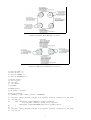
This document provides a tutorial for MoDeST, a modeling language for stochastic timed system. The syntax
and the semantics of the language will be introduced by the use of examples. There are four examples in this
document, each modeling a protocol with increasing complexity. As the complexity increases, more types of
constructs are required to model the protocols properly.
The protocols that are modeled are taken from section 3.4 of [1], Principles of Reliable Data Transfer (rdt). Figure
1 presents the service model of the rdt. The service offered by rdt to the upper layer is characterized by:
(a) No transfered data bits are corrupted,
(b) No transfered data bits are lost,
(c) All data are delivered in the order in which they are sent.
Figure 1: Reliable Data Transfer Service
Figure 1 also presents the service implementation of the rdt. Since it is not always possible to guarantee the
reliability of the layer below, the rdt must devise a protocol to ensure that the above-mentioned characteristics
are satisfied. In this tutorial we will model four of such protocols in MoDeST.
Model 1: Reliable Data Transfers Over a Perfectly Reliable Channel (rdt1.0)
The first protocol (rdt1.0 ) relies on the assumption that the lower layer satisfies all of the above-mentioned
characteristics. The service implementation of rdt1.0 is depicted in Figure 2, which shows the Finite State
Machine (FSM) diagrams of both sender and receiver.
Figure 2: Reliable Data Transfer 1.0
1
Each of sender or receiver has one state, depicted by the circles. Transitions, depicted by arrows, are triggered by
the occurrences of the events shown above the horizontal lines. Below the horizontal lines are the actions taken
when the events occur.
The model of rdt1.0 in MoDeST is as follows:
01 action rdt_send, make_pkt, udt_send,
02
rdt_rcv, extract, deliver_data;
03 int loss;
04 process sender(){
05
rdt_send; make_pkt; udt_send {= loss=1 =}
06 }
07 process receiver(){
08
rdt_rcv {= loss-=1 =}; extract; deliver_data
09 }
10 process channel(){
11
udt_send; rdt_rcv
12 }
13 par{ :: sender()
14
:: receiver()
15
:: channel()
16 }
The model consists of three processes: sender, receiver and channel. We decide not to abstract away from the channel
to allow us to model the protocols better by placing the unreliability inside the channel process. A process in MoDeST
contains statements governing the occurrences of events (actions) in the process. For instance, in process sender, three
actions occur sequentially, namely: rdt send, make pkt and udt send. Lines 01, 02 list all actions that exist in the model.
Two sequential actions are separated by ;.
In MoDeST it is possible to define constants, variables and data structures. For more information on constants, primitive
data types, data structures and operations that can be applied to them, consult [2]. Variables can be global, in which case
can be accessed by all processes, or local to a process. In our model, loss is a variable of type integer. It is defined in
line 03. The occurrences of action udt send set this variable to 1, while the occurrences of rdt rcv reduces this variable
by 1. This variable is useful to model data that are communicated among processes or to model rewards, which will be
explained further in the next section.
Lines 13-16 define a parallel composition of the three processes. All processes (actions) in a parallel compositions occur
parallelly and independent of each others. However if they share a common actions then the occurrences of these actions
are synchronized. Thus in our model, processes sender and channel synchronize on action udt send, while processes
receiver and channel synchronize on action rdt rcv.
It must be noted that we abstract away from the data aspect of the protocol (namely data and packet in Figure 2).
However, this is not a restriction. If we like, we can model the data aspect by using global variables.
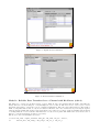
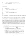
Figure 3: Creating Projects and MoDeST Models in Möbius
2
Möbius: Creating Projects and MoDeST Models
It is assumed at this point that you already have Möbius and MoTor tools installed in your systems. To create
a project and a MoDeST model follow the following steps:
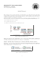
• Run the Möbius tool (MOBIUSDIR/bin/mobius &). After running it, the “Möbius Project Manager” will
be shown (Figure 3 circle 1),
• Create a new project from menu Project → New and the “Project” window will be shown (Figure 3
circle 2),
• Create a new “Atomic Model” by right-clicking the icon Atomic and choosing New in the popup menu.
The “Specify Atomic Name and Type” will be shown (Figure 3 circle 3),
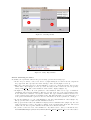
• Enter the model name and choose MoDeST Model from the list of the model types. The “Möbius Text
Editor” will be shown (Figure 4). Type your MoDeST model in the text editor.
• You can save your model from menu File → Save. Saving a model compiles it.
Figure 4: Möbius Text Editor
Model 2: Reliable Data Transfers Over a Channel with Bit Errors (rdt2.0)
The second protocol (rdt2.0 ) is built on the assumption that the lower layer satisfies all characteristics but (a), namely
the lower layer may deliver corrupted data bits. In order to tackle this problem, the receiver must posses mechanisms to
detect error and to notify the sender about its receiving status. Positive (ACK) and negative (NAK) acknowledgement
are used for the later case. The error detection is performed by incorporating checksum field in the data packet. On the
sender side, the sender must wait for either ACK or NAK of each packet that it sends and must be able to retransmit in
case of receiving NAK. For this protocol we assume that the ACK’s and NAK’s are always delivered correctly. The FSM
diagrams of both sender and receiver in rdt2.0 is depicted in Figure 5.
Figure 5: Reliable Data Transfer 2.0
The model of rdt2.0 in MoDeST is as follows:
01 action rdt_send, compute_checksum, make_pkt, udt_send_packet, rdt_rcv_NAK, rdt_rcv_ACK,
02
rdt_rcv_packet, extract, deliver_data, udt_send_NAK, udt_send_ACK;
03 const int CORRUPT = 0;
04 const int NOTCORRUPT = 1;
05 int resending;
06 int status;
3
07 process sender(){
08
rdt_send; compute_checksum; make_pkt {= resending=0 =}; udt_send_packet;
09
do{ :: rdt_rcv_NAK; udt_send_packet
10
:: rdt_rcv_ACK; break
11
}
12 }
13 process receiver(){
14
do{ ::rdt_rcv_packet;
15
alt{ :: when(status==CORRUPT) {= resending=1 =}; udt_send_NAK
16
:: when(status==NOTCORRUPT) extract; deliver_data; udt_send_ACK
17
}
18
}
19 }
20 process channel(){
21
do{ :: udt_send_packet;
22
alt{ :: {= status=CORRUPT =}; rdt_rcv_packet
23
:: {= status=NOTCORRUPT =}; rdt_rcv_packet
24
}
25
:: udt_send_NAK; rdt_rcv_NAK
26
:: udt_send_ACK; rdt_rcv_ACK
27
}
28 }
29 par{ :: sender()
30
:: receiver()
31
:: channel()
32 }
Like the previous model, the model of rdt2.0 also consists of three processes. Inspect the changes in process sender.
Firstly, this process now has an action called udt send packet instead of udt send. This is done to differenciate unreliable
data transfer for packet, ACK and NAK from each others. Secondly, a new construct, namely do{} is used. Statement do
is used to model loop. Each sequence of statements after :: is the sequence that will occur in one iteration of the loop.
The selection of the sequence to execute is performed non-deterministically. If after the :: there exists some conditions
(for instance construct when() in process receiver or synchronization with other processes) then only those sequences
whose conditions can be resolved to true will be selected. Thus in process sender after action udt send packet, sequence
rdt rcv NAK; udt send packet will occur continuously until the sequence rdt rcv ACK; break is selected, for action break
breaks the loop and the next action after the loop occurs.
In the receiver process, a similar do construct exists, with only one choice. After action rdt rcv packet occurs a new
construct, alt{} is used. This statement is used to model choices. Thus either sequence of statements after :: will be
selected. Similar to do, the sequences of statements are also guarded by conditions. In our model the corruption of data
packet by the channel is modeled by a global variable status. The process channel sets the value of this variable to
CORRUPT or NOTCORRUPT. Process receiver consults this variable and decide which choice is selected in the alt statement.
The process channel models the delivery of the data packets, ACK’s and NAK’s, which is represented by the three choices
of the do construct. In the case of delivering data packet, the channel selects to corrupt or not to corrupt the delivery
non-deterministically by setting the value of global variable status.
The three processes are put in a parallel composition in lines 29-32. Hence, processes sender and channel synchronize
on actions udt send packet, rdt rcv NAK and rdt rcv ACK, while processes receiver and channel synchronize on actions
rdt rcv packet, udt send NAK and udt send ACK.
Notice that we have a global variable resending which is set to 0 before the packet is sent and to 1 if it is received corrupt.
This variable is used to model reward and in the simulation of the model (to be explained later) can be used to measure
the average time the protocol retransmits a packet. In this model also we abstract away from modeling the data aspect of
the protocol.
Möbius: Defining Reward Variables
It is assumed that a new “Atomic Model” of rdt2.0 with the name rdt2 0 has been created. To define reward
variables for this model perform the following steps:
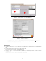
• In the “Project” window, create a new “Reward” by right-clicking the icon Reward and choosing New in
the popup menu. The “Specify Reward Name and Type” will be shown (Figure 6 circle 1),
• Enter the reward name and click OK and the “Select Reward Child” will be shown (Figure 6 circle 2).
Select the model for whom the reward is specified, namely rdt2 0, the “Reward Definition” window will
be displayed (Figure 7).
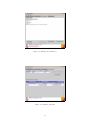
• You can add reward variables by entering their name in the textbox “Enter new variable name” and
click “Add Variable”. In Figure 7 we have added 2 variables, namely resend and n nack. The definition
of variable resend is based on state variable resending in the model, thus it is a state reward. You
4
Figure 6: Defining Reward Variables in Möbius
Figure 7: Rate Reward Variables
can see the available state variables in upper list and you can define the reward function in the textbox
below. In this case we define the variable resend to be return rdt2 0->resending->getValue(). For
each state variables in the model, its value can be obtained by getValue() function. Basically, any C
code governing some state variables of the model can be input as reward function.
• The definition of variable n nack (Figure 8) is based on the occurrence of action udt send NAK, thus it
is an impulse reward. You can select any number of actions from the upper list and then define the
impulse reward function in the textbox below. In our case the impulse reward function is return 1,
which means the occurrence of action udt send NAK will give value 1 to variable n nack. You will notice
that basically both variables resend and n nack perform the same measurement, namely the average
number of retransmission of a packet.
• Figure 9 shows the “Simulation” tab of the “Reward Definition” window. In this tab you can define the
type of the reward variable evaluations. There are four types, namely instant of time, interval of time,
time averaged interval of time and steady state. These types determine when the reward function of a
certain reward variable is evaluated when it is simulated. In this tab, it is also possible to determine
the types of estimations of certain reward variable we would like to be produced by the simulation.
There are four basic estimations available, namely mean, variance, interval and distribution. In the
“Confidence” tab, we can determine the confidence level and the confidence interval of the simulation.
For more information about these parameters, please consult [3].
5
Figure 8: Impulse Reward Variables
Figure 9: Reward Variables Simulation
Model 3: Reliable Data Transfers Over a Channel with Bit Errors (rdt2.2)
The third protocol (rdt2.2 ) is an improvement of rdt2.0. While in rdt2.0 it is assumed that the ACK’s and NAK’s are
always delivered correctly, in this protocol such assumption does not exist. To this end we need to add a sequence number
field in the data packet to enable the receiver to identify retransmissions. Since the sender always waits for either ACK or
NAK of each packet that it sends, we only need 2 values for this field. rdt2.2 also extends rdt2.0 by removing the negative
acknowledgement (NAK). The negative acknowledgement is now replaced by multiple ACK’s mechanism, namely instead
of sending NAK, the receiver sends the ACK if the last correctly received packet. The FSM of the sender and receiver of
this protocol is shown in Figure 10 and 11, respectively.
The model of rdt2.2 in MoDeST is as follows:
01 action rdt_send, compute_checksum, make_pkt, udt_send, rdt_rcv, extract,
02
deliver_data, udt_send_s, udt_send_r, rdt_rcv_s, rdt_rcv_r;
6
Figure 10: Reliable Data Transfer 2.2: Sender
Figure 11: Reliable Data Transfer 2.2: Receiver
03
04
05
06
const
const
const
const
int
int
int
int
DATA = 0;
ACK = 1;
CORRUPT = 0;
NOTCORRUPT = 1;
07 typedef struct{
08
int seq_num;
09
int type;
10
int status;
11 } PACKET;
12 PACKET packet;
13 int resend_0, resend_1;
14 process sender(){
15
PACKET p; p.type = DATA; p.status = NOTCORRUPT;
16
17
18
19
20
21
22
rdt_send; compute_checksum; make_pkt {= p.seq_num=0, packet=p, resend_0=0 =}; udt_send;
do{::rdt_rcv;
alt{::when(packet.status==CORRUPT || packet.seq_num==1)
{= p.seq_num=0, packet=p, resend_0=1 =}; udt_send
::when(packet.status==NOTCORRUPT && packet.seq_num==0) break
}
};
rdt_send; compute_checksum; make_pkt {= p.seq_num=1, packet=p, resend_1=0 =}; udt_send;
do{::rdt_rcv;
7
23
24
25
26
}
27 }
alt{::when(packet.status==CORRUPT || packet.seq_num==0)
{= p.seq_num=1, packet=p, resend_1=1 =}; udt_send
::when(packet.status==NOTCORRUPT && packet.seq_num==1) break
}
28 process receiver(){
29
PACKET p; p.type = ACK; p.status = NOTCORRUPT;
30
31
32
33
34
35
36
37
38
39
40 }
do{::rdt_rcv;
alt{::when(packet.status==CORRUPT || packet.seq_num==1) {= p.seq_num=1, packet=p =}; udt_send
::when(packet.status==NOTCORRUPT && packet.seq_num==0) extract; deliver_data; compute_checksum;
make_pkt {= p.seq_num=0, packet=p =}; udt_send; break
}
};
do{::rdt_rcv;
alt{::when(packet.status==CORRUPT || packet.seq_num==0) {= p.seq_num=0, packet=p =}; udt_send
::when(packet.status==NOTCORRUPT && packet.seq_num==1) extract; deliver_data; compute_checksum;
make_pkt {= p.seq_num=1, packet=p =}; udt_send; break
}
}
41 process channel(){
42
do{::udt_send_s;
43
palt{:98:rdt_rcv_r
44
:1:{= packet.status=CORRUPT =}; rdt_rcv_r
45
:1:{= packet.seq_num=1-packet.seq_num =}; rdt_rcv_r
46
}
47
::udt_send_r;
48
palt{:196:rdt_rcv_s
49
:2:{= packet.status=CORRUPT =}; rdt_rcv_s
50
:2:{= packet.seq_num=1-packet.seq_num =}; rdt_rcv_s
51
}
52
}
54 }
55 par{ :: relabel {udt_send, rdt_rcv} by {udt_send_s, rdt_rcv_s} hide {compute_checksum, make_pkt} sender()
56
:: relabel {udt_send, rdt_rcv} by {udt_send_r, rdt_rcv_r} hide {compute_checksum, make_pkt} receiver()
57
:: channel()
58 }
In the model of rdt2.2 above we make use of the data structure struct to define a packet. A packet in the model consists
of a sequence number, a type - a DATA or a ACK packet, and a status. Thus the data field as well as the checksum are not
modeled. The inconsistency of the data and checksum fields are modeled by the channel setting the status field of the
packet to CORRUPT.
In process sender for each value of sequence number, upon receiving a packet from the upper layer and preparing it for
delivery, the sender continuously sends the packet if the status or the sequence number of the expected ACK is not correct.
The same case is also performed in process receiver: for each value of sequence number, upon receiving a packet from the
lower layer, the receiver prepares and sends an ACK with sequence number adjusted according to the status and sequence
number of the packet it receives.
A new construct is used in process channel, namely palt. This construct models a probabilistic alternative. After the
occurrences of action udt send r or udt send s, the first choice is selected with probability 98/100 while the second and
the third choices are selected with probability 1/100 each. Thus in our model, the channel corrupts the packet and flips
the sequence number of the packet each with probability 0.01.
In the parallel composition of the three processes, we make use of statements relabel and hide. relabel renames the
listed actions in the process. For instance, actions udt send and rdt rcv of process sender are renamed as udt send s
and rdt rcv s respectively. Statement hide hides the listed actions from the environment of the process, hence hindering
them from being used in synchronization. Note that we do not wish to have processes sender and receiver to synchronize
on actions compute checksum or make packet.
We also have two global variables resend 0 and resend 1 in the model. These variables can be used to measure the
retransmission for each sequence number in the simulation.
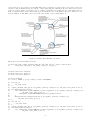
Model 4: Reliable Data Transfers Over a Lossy Channel with Bit Errors (rdt3.0)
An extension of protocol rdt2.2 to address a lossy lower layer is given by protocol rdt3.0. The sender detects a packet loss
by the absence of ACK for the packet after an interval of time has passed. Such interval of time, called timeout, is selected
8
by the sender based on a prediction of Round Trip Time and processing time of packets in the receiver. Since a packet can
experience a large transmission delay, the existence of timeout may introduce duplication. However, this is not a problem,
for the use sequence number enables the receiver to identify retransmission. Note that since the sender always waits for
ACK of each packet that it sends, characteristic (c) is also satisfied by rdt3.0. The FSM of the sender of this protocol is
depicted in Figure 12. The FSM of the receiver is the same as that of rdt2.2, namely Figure 11.
Figure 12: Reliable Data Transfer 3.0: Sender
The model of rdt3.0 in MoDeST is as follows:
01 action rdt_send, compute_checksum, make_pkt, udt_send, rdt_rcv, extract, deliver_data,
02
start_timer, udt_send_s, udt_send_r, rdt_rcv_s, rdt_rcv_r;
..
14 extern const float timeout=2;
15 extern const float lprop=0.5;
16 extern const float uprop=1.1;
17 process sender(){
18
clock x; PACKET p; p.type = DATA; p.status = NOTCORRUPT;
19
20
21
22
23
24
25
26
27
28
29
30
31
32
33
34
do{::rdt_rcv
::rdt_send; break
};
compute_checksum; make_pkt {= p.seq_num=0, packet=p, resend_0=0 =}; udt_send; start_timer {= x=0 =};
do{::when(x<timeout) rdt_rcv;
alt{::when(packet.status==CORRUPT || packet.seq_num==1) {= p.seq_num=0, packet=p, resend_0=1 =};
udt_send; start_timer {= x=0 =}
::when(packet.status==NOTCORRUPT && packet.seq_num==0) break
}
::when(x>=timeout) urgent(x>=timeout) {= p.seq_num=0, packet=p, resend_0=1 =};
udt_send; start_timer {= x=0 =}
};
do{::rdt_rcv
:: rdt_send; break
};
compute_checksum; make_pkt {= p.seq_num=1, packet=p, resend_1=0 =}; udt_send; start_timer {= x=0 =};
do{::when(x<timeout) rdt_rcv;
alt{::when(packet.status==CORRUPT || packet.seq_num==0) {= p.seq_num=1, packet=p, resend_1=1 =};
udt_send; start_timer {= x=0 =}
9
35
36
37
::when(packet.status==NOTCORRUPT && packet.seq_num==1) break
}
::when(x>=timeout) urgent(x>=timeout) {= p.seq_num=1, packet=p, resend_1=1 =};
udt_send; start_timer {= x=0 =}
38
}
39 }
..
51 process channel(){
52
clock x; float prop;
53
do{::udt_send_s {= x=0, prop=Uniform(lprop,uprop) =}; when(x>=lprop) urgent(x>=prop)
54
palt{:97:rdt_rcv_r
55
:1:{= packet.status=CORRUPT =}; rdt_rcv_r
56
:1:{= packet.seq_num=1-packet.seq_num =}; rdt_rcv_r
57
:1:tau
58
}
59
::udt_send_r {= x=0, prop=Uniform(lprop,uprop) =}; when(x>=lprop) urgent(x>=prop)
60
palt{:97:rdt_rcv_s
61
:1:{= packet.status=CORRUPT =}; rdt_rcv_s
62
:1:{= packet.seq_num=1-packet.seq_num =}; rdt_rcv_s
63
:1:tau
64
}
65
}
66 }
67 par{::relabel {udt_send, rdt_rcv} by {udt_send_s, rdt_rcv_s} hide {compute_checksum, make_pkt} sender()
68
::relabel {udt_send, rdt_rcv} by {udt_send_r, rdt_rcv_r} hide {compute_checksum, make_pkt} receiver()
69
::channel()
70 }
To model the timeout in rdt3.0 we use the variable of type clock in MoDeST. A clock is variable whose value is increasing
continuously modeling the advances of time. In process sender, for each sequence number, right after a packet is sent, a
clock x is reset. There are two choices in the do construct right now. The first can be selected as long as the value of
clock x is less than timeout, which is done by using statement when(). Notice that a new construct urgent() is being
used. This construct forces the occurrence of the next action once the value of its condition resolves to true. Thus, for
instance in process channel, constructs when(x>=lprop) urgent(x>=prop) indicate that the next action must occur when
the value of clock x is within interval [lprop,prop]. In process sender retransmission occurs when the received ACK is
corrupted or has an incorrect sequence number or the timeout has expired.
Note that we model the propagation and processing delays in the channel by using clock x. The value of variable prop,
representing the upper bound of the interval of these delays, is taken from the Uniform distribution. A value of a float
variables can also be taken from other distributions. For more information about the distributions that can be used,
consult [2]. The statement :1:tau in the palt construct represents a packet loss.
In this model we define three variables timeout, lprop and uprop to be external. The value of these variables are supplied
by the environment. This is useful when we wish to experiment with several studies (to be explained below) in the
simulation of the model in Möbius. In the declaration of this variables in lines 14-16, they are also initialized. These
initial values are their default values.
The model of process receiver is omitted from the code, for it is the same as that of rdt2.2.
Möbius: Creating Studies
It is assumed that a new “Atomic Model” of rdt3.0 with the name rdt3 0 has been created. Two state rewards
have also been defined in the reward model with the name reward rdt3 0. To create studies for this model
perform the following steps:
• In the “Project” window, create a new “Study” by right-clicking the icon Study and choosing New in the
popup menu. The “Specify Study Name and Type” will be shown (Figure 13 circle 1).
• Enter the study name and select “Set Study” as the type. Click OK and the “Select Study Child”
will be shown (Figure 13 circle 2). Select the reward model for whom the study is specified, namely
reward rdt3 0. The “Study Definition” window will be displayed (Figure 14).
• In Figure 14, you can see all of external variables defined in the model listed. For all these variables,
you can define some sets of experiments by assigning them values for each experiment. We have defined
two experiments. You can add more experiments by clicking the “Add” button. You can also activate
and deactivate certain experiments by clicking “Experiment Activator” button. Defining our studies this
way, we will have two experiments in the simulation with different parameters.
• The study type we have selected is the ‘Set Study”. Möbius also provides “Range Study” type. With this
type, it is possible to assign values to each variable in different ways, namely incrementally, functionally,
manually and randomly. For more information on “Range Study” type, consult [3].
10
Figure 13: Creating Studies
Figure 14: Study: Experiments
Möbius: Simulating the Model
To simulate the experiments defined in the previous study, perform the following steps:
• In the “Project” window, create a new “Solver” by right-clicking the icon Solver and choosing New in
the popup menu. The “Specify Solver Name and Type” will be shown (Figure 15 circle 1).
• Enter the solver name and select “Mobius Simulator” as the type. Click OK and the “Select Solver
Child” will be shown (Figure 15 circle 2). Select the study model for whom the solver is specified,
namely study rdt3 0. The “Solver Definition” window will be displayed (Figure 16).
• In Figure 16, you can see all of the parameters of the simulation. There are two type of simulation:
terminating and steady-state simulation. This type depends on the type of the reward variables in the
model, which can be transient or steady-state rewards. Two types of Random Number Generator are
provided, namely Lagged Fibonacci and Tauseworthe. The Random Number seed determines the seed
of the pseudo-random number generators. For more information about these parameters, consult [3].
• To run the simulation, go to tab “Run Simulation” and click “Start Simulation” button (Figure 17).
The project files will be compiled and the simulation is started.
• The progress and the result of the simulation is displayed in tab “Simulation Info” (Figure 18). For each
defined experiment you can see the result by clicking on the experiment name in the list. The reward
variables are also listed, together with their mean values and confidence intervals.
• If you have set the trace level of the simulation to any values but zero, then you can find the trace
file in MOBIUSPROJECT/projname/Solver/simname/Results expname compname trace.txt. The result of
11
Figure 15: Creating Simulators for MoDeST Models
Figure 16: Simulation Parameters
the simulation is also saved in file MOBIUSPROJECT/projname/Solver/simname/Results results.txt.
Inverst some time to inspect the trace files.
References
[1]
J. F. Kurose and K. W. Ross. Computer Networking: A Top-Down Approach Featuring the Internet. Addison-Wesley,
2001.
[2]
R. Klaren. MoDeST Language Manual. Universiteit Twente, 2005.
http://fmt.cs.utwente.nl/tools/motor/manual/manual.ps.gz
[3]
Anonymous. Möbius: User Manual. Performability Engineering Research Group, University of Illinois at UrbanaChampaign, 2005.
http://www.perform.csl.uiuc.edu/mobius/manual/MobiusManual.pdf
12
Figure 17: Running the Simulation
Figure 18: Simulation Results
13