1
ISSN 0280-5316
ISRN LUTFD2/TFRT--5736--SE
Modeling and Control of the
Ball and Beam Process
Marta Virseda
Department of Automatic Control
Lund Institute of Technology
March 2004
Department of Automatic Control
Lund Institute of Technology
Box 118
SE-221 00 Lund Sweden
Document name
MASTER THESIS
Date of issue
March 2004
Document Number
ISRNLUTFD2/TFRT--5736--SE
Author(s)
Supervisor
Marta Virseda
Rolf Johansson and Anders Robertsson at LTH in Lund.
Enrique Baeyens at Univ. de Valladolid in Spain
Sponsoring organization
Title and subtitle
Modeling and Control of the Ball and Beam Process (Modellering, simulering och reglering av kula på bom processen).
Abstract
One of the most difficult problems that an engineer who works with modeling deals
with, is the question about how to translate a physical phenomenon into a set of
equations. It is usually difficult to capture all dynamics and phenomena, so one
usually strives for a set of equations that describes the physical system
approximately and adequately with the accuracy for the purpose. In our case, we
model the dynamics relevant for control design.
The topic of this thesis was to do an in-depth study of the Ball and Beam
process. Two different experimental implementation of the Ball and Beam process
have been considered, both available at the course lab at the Department of
Automatic Control, Lund. The first step consisted of deriving the equations of
motion, that is, to do the mathematical modeling of the process.
In order to implement this model Modelica has been used. Modelica, which is a
powerful language for modeling of physical systems, uses the tool Dymola. Another
model was designed also with Modelica but with the help of the extension of the
multi body library, which uses a methodology based on object orientation and
symbolic manipulation of equations. With this last model it was possible to
visualize an animation in real time 3D.
The following step of the project was to do control design for the different
models. The obtained simulations were shown in Dymola and Simulink.
Finally experiments on the real process were developed, based on vision feedback.
Keywords
Modeling, control, object-oriented modeling
Classification system and/or index terms (if any)
Supplementary bibliographical information
ISSN and key title
ISBN
0280-5316
Language
Number of pages
English
47
Recipient’s notes
Security classification
The report may be ordered from the Department of Automatic Control or borrowed through:University Library, Box 3, SE-221 00 Lund, Sweden Fax +46 46
222 42 43
Acknowledgments
This work has been accomplished at the Department of Automatic Control at Lund
Institute of Technology in Sweden, between October 2003 and March 2004.
Initially, I would like to express my gratitude to Dr. Rolf Johansson for giving the
possibility to work in this department under his supervision.
I wish to express my sincere gratitude to Anders Robertsson, who guided this thesis and
helped whenever I was in need. He helped me with my doubts and questions.
I wish to thank all my Spanish friends for their inspirational and moral support and
especially to my friends Raul and Tania who helped me in my earlier days when I arrived to
Sweden.
Last but certainly not least, I would like to show my gratitude to my parents, my sister and
my grandparents who have been generous with their encouragement.
This thesis is dedicated to them.
TABLE OF CONTENTS
Introduction................................................................................................................................... 1
Dymola and Modelica ................................................................................................................... 2
2.1
Dymola ........................................................................................................................... 2
2.1.1
Dymola features ...................................................................................................... 3
2.1.2
The modeling environment ..................................................................................... 4
2.2
Modelica......................................................................................................................... 4
2.2.1
Modelica features.................................................................................................... 5
2.3
How to learn Dymola and Modelica........................................................................... 8
Ball and Beam ............................................................................................................................... 9
3.1
Process Description....................................................................................................... 9
Mathematical modeling .............................................................................................................. 12
4.1
Ball and Beam Model.................................................................................................. 12
4.1.1
Newton’s second law ............................................................................................ 12
4.1.2
Lagrangian methods.............................................................................................. 14
Modeling in Modelica ................................................................................................................. 19
5.1
Models with Modelica language ................................................................................ 19
5.1.1
Modelica model: Newton’s second law................................................................ 20
5.1.2
Modelica model: Lagrangian method ................................................................... 21
5.2
Model with Modelica’s libraries ................................................................................ 23
Control Design and Simulations ................................................................................................ 26
6.1
Control design ............................................................................................................. 26
6.1.1
Control design: linear observer-based control ...................................................... 26
6.1.2
Control Design: nonlinear system......................................................................... 28
6.2
Simulations .................................................................................................................. 31
6.2.1
Simulations in Simulink........................................................................................ 31
Experiments................................................................................................................................. 33
7.1
7.2
Experimental Setup .................................................................................................... 33
How to do the experiments......................................................................................... 34
Conclusions.................................................................................................................................. 42
8.1
Conclusions.................................................................................................................. 42
Chapter 1
Introduction
This thesis concentrates on the study of the Ball and Beam process. The modeling has been
done with Modelica and Dymola.
Dymola is an integrated environment for developing models in the Modelica language and
a simulation environment for performing experiments.
To do the control design there are many possibilities; this project presents an observerbased control design development in Matlab based on pole-placement. The simulations are made
in Simulink and Dymola. The experiments with the real Ball and Beam process are done with the
controller implemented in a real-time extension to Simulink and viasual feedback from a camera
system.
A short description of the thesis chapter is outlined below:
Chapter 2 presents an explanation of different tools used for the modeling.
Chapter 3 describes the study of the Ball and Beam process.
Chapter 4 presents the mathematical modeling of the physical system.
Chapter 5 gives the modeling in Modelica of the beam and ball process.
Chapter 6 contains control design of the obtained models and the corresponding
simulations.
Chapter 7 contains the experiments done.
Chapter 8 presents the summarized conclusions of this thesis.
1
Chapter 2
Dymola and Modelica
This chapter gives a short introduction to the different tools used for the modeling in the
thesis.
2.1 Dymola
The company Dynasim's mission is to develop the software tools that industry needs for
solving demanding modeling, simulation and design problems. The emphasis is on handling
large, multi-engineering systems efficiently. Dymola pioneered the object-oriented physical
modeling methodology and the accompanying simulation technology.
In 1996, Dynasim took the initiative to design a new unified object-oriented language for
physical systems modeling, called Modelica. Founded in 1992, Dynasim is the leading developer
and implement of object-oriented multi-engineering modeling technology and the Modelica
language [2].
Dymola - Dynamic Modeling Laboratory - is a tool for multi-domain modeling and
simulation. Dynasim developed it. Dymola supports the modeling language Modelica for which,
there are a number of free and commercial model libraries that include models of mechanical,
thermal, hydraulic, and thermodynamic and control systems. [4]
Dymola uses a new modeling methodology based on object orientation and symbolic
manipulation of equations. The usual need for the manual conversion of equations to a block
diagram is removed by the use of automatic formula manipulation.
2
Chapter 2. Dymola and Modelica
2.1.1 Dymola features:
¾ Model Translator
Automatic causality analysis
Symbolic solution of equations and index reduction
Solution of algebraic loops
Automatic handling of time and state events
Generate C-code
¾ Handles large, complex multi-domain models
¾ Faster modeling by graphical model composition
Graphical model editor and browser
Drag submodels from libraries
Parameter forms
Connect graphically
Build icons - polygons, circles, text, color etc…
Text editor for declarations and equations
Automatic HTML model documentation
¾ No manual equation manipulation needed
¾ Faster simulation - symbolic pre-processing
¾ Open for user defined model components
¾ Open interface to other programs
¾ Animation
Real time 3D animation
Boxes, spheres, cylinders, etc - predefined visual classes
Import of DXF and STL files
Hidden surface removal, shading
Plotting
¾ Simulator
Handles ODE and DAE models
State or the art numerical integration
Flexible initialization
Interface to external C-functions
Matlab/Simulink, xPC an d SPACE interfaces
DDE interface
Real time simulation [1]
3
Chapter 2. Dymola and Modelica
2.1.2 The modeling environment
Dymola is an integrated environment for developing models in the Modelica language and
a simulation environment for performing experiments.
The Dymola modeling environment is divided in two main parts:
¾ At the modeling mode called, Model Editor, where the models are composed from
library components (from the Modelica standard library, other libraries, and
commercial and proprietary libraries) as well as models developed by the user. Models
are either composed of other, more primitive, components, or described by equations at
the lowest level.
This mode allows:
Model composition
Default parameter settings
Definition of equations
¾ At the simulation mode, Dymola transforms a declarative, equation based, model
description into efficient code. In this level it is possible show the results as animations
or using plot windows for visualization of simulation results.
Dymola provides a complete simulation environment, but can also export code for
simulation in Simulink. In addition to the usual offline simulation, Dymola can generate code for
specialized hardware-in-loop systems, such as, dSPACE, xPC and others [5].
Dymola uses Modelica, which is an object orientated modeling language, which supports
hierarchical structuring, reuse and evolution of large and complex models independent from the
application. It uses acausal modeling based on differential and algebraic equations.
2.2 Modelica
Modelica [3] is a powerful language for modeling of physical systems designed to support
effective library development and model exchange. It is a modern language built on acausal
modeling with mathematical equations and object-oriented constructs to facilitate reuse of
modeling knowledge.
The work with Modelica started in September 1996 with a group of about fifteen persons
with knowledge about modeling languages and models with differential algebraic equations
(DAE).
The first version of the Modelica language definition was finished in September 1997. In
January 2002 a new version was released.
4
Chapter 2. Dymola and Modelica
2.2.1
Modelica features
The four most important features of Modelica are:
¾ Is based on equations instead of assignment statements. This permits acausal
modeling that gives better reuse of classes since equations do not specify a certain
data flow direction. Thus a Modelica class can adapt to more than one data flow
context.
¾ Has multi-domain capability, meaning that model components corresponding to
physical objects from several different domains such as e.g. electrical, mechanical,
thermodynamic, hydraulic, biological and control applications can be described and
connected.
¾ Is an object-oriented language with a general class concept that unifies classes,
generics, and general subtyping into a single language construct. This facilitates reuse
of components and evolution of models.
¾ Has a strong software component model, with constructs for creating and connecting
components. Thus the language is ideally suited as an architectural description
language for complex physical systems, and to some extend for software systems.
Models and sub-models are declared as classes with connection interfaces called
connectors. This connection capability allows the use of model libraries to compose complex
models with the drag and drop and connection drawing facilities of modern graphical editors.
The goal of the Modelica design effort is to design physical systems modeling language
that makes life for the model builders considerably easier and more productive.
Following are described the general features of Modelica.
Hierarchical modeling
Modelica supports both high levels modeling by composition and detailed library
component modeling by equations. Models of standard components are typically available in
model libraries. Using a graphical model editor, a model can be defined by drawing a
composition diagram by positioning icons that represent the models of the components, drawing
connections and giving parameter values in dialogue boxes. Constructs for including graphical
annotations in Modelica make icons and composition diagrams portable between different tools
[2].
5
Chapter 2. Dymola and Modelica
An example of the textual representation of a simple motor drive system is:
model MotorDrive
PID
controller:
Motor
motor;
Gearbox gear (n=100);
Inertia
inertia
(J=10);
equation
connect(controller.outPort, motor.inPort);
connect(controller.inPort2, motor.outPort);
connect(gear.flange_a
, motor.flange_b);
connect(gear.flange_b , inertia.flange_a);
end MotorDrive;
The composition diagram of the model class Motor is shown below:
Figure 2.1: Motor drive with Modelica libraries
6
Chapter 2. Dymola and Modelica
Structure model libraries
A powerful package concept is available to structure large model libraries and to find a
component in a file system giving its hierarchical Modelica class name.
Hybrid modeling
A unique feature of Modelica is the handling of discontinuous and variable structure
components such as relays, switches, bearing friction, clutches, brakes, impact, sampled data
systems, automatic gearboxes etc. Modelica has introduced special language constructs allowing
a simulator to introduce efficient handling of events needed in such cases.
Array
Modelica supports arrays, utilizing a Matlab like syntax. The elements of arrays may be
of the basic data types (Real, Integer, Boolean, String) or component models. This allows
convenient discretization of simple partial differential equations.
Class parameters
Besides ordinary numeric parameters, Modelica allows model class parameters. As an
example assume that an auto-tuning controller should replace a PI controller. It is of course
possible to just replace the controller in a graphical user environment, i.e., to create a new model.
The problem with this solution is that two models must be maintained. Modelica has the
capability to instead substitute a model component so only one version of the rest of the model is
needed.
Equations
Models in Modelica are mathematically described by differential, algebraic and discrete
equations. No particular variable needs to be solved manually. A Modelica tool will have enough
information to decide it automatically. Modelica is designed such that available, specialized
algorithms can be utilized to enable efficient handling of large models having more than hundred
thousand equations. Modelica is suited and used for hardware-in-the-loop simulations and for
embedded control systems.
7
Chapter 2. Dymola and Modelica
2.3
How to learn Dymola and Modelica
The first task of this thesis was learning Dymola and the Modelica language. In my
computer version (5.1) of Dymola was installed, available as free source code. Most of the
existing tutorials are based on examples, besides I used several tutorials and books, some of them
were:
¾ The guide “Getting Started with Dymola” [1] included in Dymola user’s manual which
provides some examples in order to guide you through Dymola. For detailed
information about the program, you can consult the on-line documentation available in
the Help menu, after selecting Documentation.
¾ The book “Introduction to Physical Modeling with Modelica” [6], which introduces to
the Modelica modeling language and shows the use the powerful features of the
Modelica language.
¾ A tutorial package called “Beginner tutorial” [7], which contains exercises. These
exercises are good to learn to write simple models, the use the Modelica standard
library etc…
¾ Modelica tutorial document and Modelica specification document, both define the
Modelica language [8].
¾ Advanced Tutorial is a continuation of Beginner tutorial [9].
8
Chapter 3
Ball and Beam
This chapter gives an introduction to the process of the ball rolling on the beam.
3.1 Process Description
The ball and beam system is one of the most enduringly popular and important laboratory
models for teaching control systems engineering. The ball and beam is widely used because it is
very simple to understand as a system, and yet the control techniques that can be studied it cover
many important classical and modern design methods. It has a very important property; it is open
loop unstable.
Figure 3.1: Diagram of Ball and Beam
9
Chapter 3. Ball and Beam
The system is very simple, a steel ball rolling on the top of a long beam. The beam is
mounted on the output shaft of an electrical motor and so the beam can be tilted about its center
axis by applying an electrical control signal to the motor amplifier.
The control job is to automatically regulate the position of the ball on the beam by
changing the angle of the beam. This is a difficult control task because the ball does not stay in
one place on the beam but moves with acceleration that is approximately proportional to the tilt
of the beam. In control terminology the system is open loop unstable because the system output
(the ball position) increases without limit for a fixed input (beam angle). Feedback control must
be used to stabilize the system and to keep the ball in a desired position on the beam.
Two different implementations of the Ball and Beam process have been considered, both
available at the course lab of the Department of Automatic Control, see figure 3.2 and 3.3.
Figure 3.2: Ball and Beam connected via gearbox
The beam is connected to a velocity controlled DC-motor via a gearbox. This makes it
much easier to control the process and there is very little influence of the cross-couplings from
the ball to the beam.
10
Chapter 3. Ball and Beam
Figure 3.3: Ball and Beam directly connected to the axis of a DC-motor
Direct driven beam: The beam is directly connected to the axis of a DC-motor.
The beam angle is measured but not the angular velocity. The ball position needs also to be
measured and in the standard configuration of the process at the Department of Automatic
Control the metal ball closes an electrical circuit along the rail of the beam.
In our experimental setup, see chapter 7, we have used a vision system for determining the
ball position. The speed of the ball needs to be estimated.
11
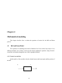
Chapter 4
Mathematical modeling
This chapter describes how to obtain the equations of motion for the Ball and Beam
process.
4.1
Ball and Beam Model
The equations for obtaining the model in Modelica have been realized by means of two
different methods. One of them is derived with simple mathematic equations using Newton’s
second law and another through the use of the Lagrangian Method.
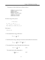
4.1.1 Newton’s second law
In this model we first consider only the relation between the beam angle and the position of
the ball.
α
x
12
Chapter 4: Mathematical modeling
The parameters of the ball and beam are defined as follows:
α
L
m
R
J
G
x
Î Beam angle coordinate
Î Beam Length
Î Mass of the ball
Î Radius of the ball
Î Ball’s moment of inertia
Î Gravitational acceleration
Î Position of the ball
Neglecting frictional forces, the two forces influencing the motion of the ball are:
-
Ftx Force due to translational motion
Frx Force due to ball rotation
Translational:
&x& =
d 2x
dt 2
Ftx = m ⋅ &x&
(4.1)
Torque due to the ball rotation is:
⎛v ⎞
⎛ x⎞
d⎜ b ⎟
d 2⎜ ⎟
dw
J
R
R
Tr = Frx ⋅ R = J ⋅ b = J ⋅ ⎝ ⎠ = J ⋅ ⎝ 2 ⎠ = ⋅ &x&
dt
R
dt
dt
Frx =
(4.2)
J
⋅ &x&
R2
13
Chapter 4: Mathematical modeling
The moment inertia of the ball is (sphere):
J=
(4.3)
2
⋅ m ⋅ R2
5
Substituting the equation (4.3) into the equation (4.2), we get:
Frx =
2
⋅ m ⋅ &x&
5
Newton’s second law along the inclination:
(4.4)
Frx + Ftx = m ⋅ g ⋅ sin α
Substituting in the equation (4.4):
2
⋅ m ⋅ &x& + m ⋅ &x& = m ⋅ g ⋅ sin α
5
In conclusion, we have:
&x& =
5
⋅ g ⋅ sin α
7
In this derivation we have taken into consideration how the ball position affects the angle
α.
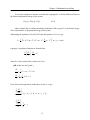
4.1.2 Lagrangian methods
The control objective is to control the torque τ applied at the pivot of the beam, such that
the ball can roll on the beam and track a desired trajectory. The torque causes thus a change of
the beam angle and a movement in the position of the ball.
τ
θb
rb
14
Chapter 4: Mathematical modeling
The parameters of the ball and beam are defined as follows:
Ib Î Beam’s moment of inertia
θb Î Beam angle
ms Î Mass of the ball
Is Î Ball’s moment of inertia
rs Î Radius of the sphere
rb Î Position of the ball
The kinetic energy of the system is:
T = Tbeam + Tsphere
Tbeam = (Tbeam ) frame + (Tbeam ) beam _ body _ center
Tsphere = (Tsphere ) frame + (Tsphere ) beam _ body _ center
Each energy is:
(Tbeam ) frame = 0
¾ The rotational kinetic energy of the beam is:
1
Tbeam ,center = ⋅ I b ⋅θ&b2
2
¾ The ball has kinetic energy with respect to the frame in both radial and circular motion:
Tsphere, frame =
(
)
1
1
⋅ ms ⋅ rb2 ⋅θ&b2 + ⋅ ms ⋅ r&b2
2
2
¾ The rotational kinetic energy of the sphere about its body center,
1
Tsphere,center = ⋅ I s ⋅θ&s2
2
(4.5)
The rotational inertia of the rolling sphere is
(4.)
2
I s = ⋅ (ms ⋅ rs2 )
5
15
(4.6)
Chapter 4: Mathematical modeling
and applying a rolling without slipping:
(4.)
r&b = rs ⋅θ&s
(4.7 )
Substituting the equations (4.6) and (4.7) into the equation (4.5), we get:
Tsphere,center =
(
1 ⎡2
⋅ ⋅ ms ⋅ rb2
2 ⎢⎣ 5
)⎤⎥ ⋅ ⎡⎢ r1 ⋅ r&
⎦ ⎣
2
s
2
b
⎤ 1 ⎡2
2⎤
⎥ = ⎢ ⋅ ms ⋅ r&b ⎥
⎦
⎦ 2 ⎣5
(4.)
The kinetic energy of the system is:
(4.6)
T=
(
)
1 ⎡
2
⎤
⋅ ⎢ I b ⋅θ&b2 + ms ⋅ rb2 ⋅θ&b2 + ms ⋅ r&b2 + ⋅ ms ⋅ r&b2 ⎥
2 ⎣
5
⎦
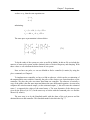
Simplifying the equation (4.8), we have:
T=
(
)
1 ⎡
7
⎤
⋅ ⎢ I b + ms ⋅ rb2 ⋅θ&b2 + ⋅ ms ⋅ r&b2 ⎥
2 ⎣
5
⎦
The rolling ball alone exhibits the potential energy of the system:
V = ms ⋅ g ⋅ rb ⋅ sin θ b
To sum up:
¾ KINETIC ENERGY
T=
(
)
1 ⎡
7
⎤
⋅ ⎢ I b + ms ⋅ rb2 ⋅θ&b2 + ⋅ ms ⋅ r&b2 ⎥
2 ⎣
5
⎦
(4.)
(4.9)
¾ POTENTIAL ENERGY
(4.)
(4.10)
V = ms ⋅ g ⋅ rb ⋅ sin θ b
16
(4.8)
(4.)
Chapter 4: Mathematical modeling
To write the equations of motion, we define the Lagrangian L, to be the difference between
the kinetic and potential energy of the system.
L(q, q& ) = T (q, q& ) − V (q )
(4.11)
where q denote the so-called generalized coordinates of the system, T is the kinetic energy
of the system and V is the potential energy of the system.
Substituting the equations (4.9) and (4.10) into the equation (4.11), we get:
L=
(
)
1 ⎡
2
⎤
⋅ ⎢ I b ⋅θ&b2 + ms ⋅ rb2 ⋅θ&b2 + ms ⋅ r&b2 + ⋅ ms ⋅ r&b2 ⎥ − ms ⋅ g ⋅ rb ⋅ sin θ b
2 ⎣
5
⎦
Lagrange’s equations of motion are formed from:
d ⎡ ∂L ⎤ ∂L
= Fqi
⎢
⎥−
dt ⎣ ∂q& i ⎦ ∂qi
where Fqi is the external force, in this case Fqi is τ.
qiÎ in this case are θb and r&b
∂L 1
= ⋅ ( I b + ms ⋅ rb2 ) ⋅ 2 ⋅θ&b
&
∂θ b 2
∂L 1 7
= ⋅ ( ⋅ 2 ⋅ ms ⋅ rb )
∂r&b 2 5
If we derive both expressions with respect to time t, we get:
⎡ ∂L ⎤
d⎢
& ⎥
⎣ ∂θ b ⎦ = ( I + m ⋅ r 2 ) ⋅θ&& + 2 ⋅ m ⋅ r ⋅ r& ⋅θ&
b
s
b
b
s
b
b
b
dt
⎡ ∂L ⎤
d⎢ ⎥
⎣ ∂r&b ⎦ = 7 m ⋅ &r&
s
b
dt
5
17
Chapter 4: Mathematical modeling
The others equations, which we need are:
∂L
= −ms ⋅ g ⋅ rb ⋅ cosθ b
∂θ b
[
]
∂L 1
= ⋅ 2 ⋅ ms ⋅ rb ⋅θ&b2 − ms ⋅ g ⋅ sin θ b
∂rb 2
EQUATIONS OF MOTION:
( I b + ms ⋅ rb2 ) ⋅θ&&b + 2 ⋅ ms ⋅ rb ⋅ r&b ⋅θ&b + ms ⋅ g ⋅ rb ⋅ cosθ b = τ
5
&r&b + ⋅ ( g ⋅ sin θ b − rb ⋅θ&b2 ) = 0
7
where τ is the torque applied to the beam.
18
Chapter 5
Modeling in Modelica
In this chapter the two models are written in the Modelica language through equations and
another model is created with the Modelica’s libraries. We also present simulation results using
Dymola for the different models.
5.1 Models with the Modelica language
Modelica is unlike most general-purpose languages not primarily based on algorithms, but
uses equations instead, that is one does not need to reformulate the differential equation into the
standard form (explicit)
dx
= f ( x, u , t )
dt
but can have general equations where the time derivatives appear implicitly. For every model the
programmer can define a number of equations describing the properties of the model. The
equations define the relation between the different quantities in the simulation.
The main reason why Modelica uses equation is that every simulation problem in fact is a
mathematical problem. It also give the language a high abstraction level, because an equation is
often more intuitive than an algorithm.
Dymola provides a complete simulation environment. Dymola transforms a declarative,
equation based, model description into efficient code. After a model has been translated into
simulation code, the simulation run is set up. Parameters and initial conditions are be defined, as
well as the duration of the simulation.
19
Chapter 5. Model in Modelica
Dymola is used to visualize dynamic behavior. Plots of the time-response of variables are
often hard to interpret and a more realistic graphical view is needed. Dymola supports a 3dimensional animated model view in addition to dynamic modeling with a library of graphical
objects. When a model is described in Dymola with equations and submodels, it is also possible
to define its visual appearance. This is done including predefined graphical objects of various
shapes.
The two obtained models in the previous chapter can be written in Modelica through their
equations of motion. These two programs are shown below with the respective simulations done
with Dymola.
5.1.1
Modelica model: Newton’s second law
model ball_beam_1
import Modelica.SIunits;
// Constants
constant Real g=Modelica.Constants.g_n "Gravitational Acceleration";
// Parameters
parameter Real k=1.0 "Motor constant";
// Variables
Real alpha "Beam angle";
Real v "Velocity of the ball";
Real a "Acceleration of the ball";
Real x "Position of the ball";
Real u "Control signal";
equation
v = der(x);
a = der(v);
// Mathematical modeling
a = (5/7)*g*Modelica.Math.sin(alpha);
der(alpha) = k*u;
// Control signal
u = 0;
end ball_beam_1;
20
Chapter 5. Model in Modelica
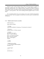
Figure 5.1: Dymola simulation: Response of beam angle, position of the ball and velocity openloop response for model base on Newton’s second law
This model fits well the beam, which is driven via a gearbox, that is the ball position, and
the torque the ball causes, does not affect the angle of the beam.
5.1.2 Modelica model: Lagrangian method
model ball_beam_2
import Modelica.SIunits;
// Parameters
parameter SIunits.Mass m=0.1 "Mass of ball";
parameter SIunits.Length L=1.0 "Beam length";
parameter SIunits.Radius r=0.015 "Radius of the ball";
parameter SIunits.MomentOfInertia J=(2/5)*m*r^2 "Sphere's moment of Inertia";
parameter SIunits.MomentOfInertia I=1e7 "Beam Inertia, value";
// Constants
constant Real g=Modelica.Constants.g_n "Gravitational Acceleration";
// Variables
Real theta "Beam Angle";
Real w "Angular Velocity";
Real alpha "Angular Acceleration";
Real x(start=0.0) "Position the ball in the beam";
Real v "Velocity of the ball";
Real a "Acceleration of the ball";
Real tau(start=0.0) "Torque";
equation
21
Chapter 5. Model in Modelica
v = der(x);
a = der(v);
w = der(theta);
alpha = der(w);
// Lagrangian method
(I + m*x^2)*alpha + 2*m*x*v*w + m*g*x*Modelica.Math.cos(theta) = tau;
a + (5/7)*(g*Modelica.Math.sin(theta) - x*w^2) = 0;
// Control law
tau = 0;
end ball_beam_2;
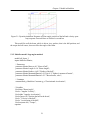
Figure 5.2: Dymola simulation: Response of beam angle, position of the ball and velocity Openloop response for the Lagrangian model
This model is appropriate for a beam, which is direct-driven from the motor (no gearbox)
and easy to move by hand. Therefore the ball position and the corresponding torque due to
gravity will affect the beam angle much more.
Both models can be exported to Simulink for either simulation or control design, which is
later to be used for the control of the beam and ball process through feedback from a vision
system. With this program, running on another computer, we can determine the ball position,
which are then sent to the controller via a network connection.
The export of a linearized model to Simulink can be realized from mode Simulation of
Dymola. In order to do it, you can use the command Linearize, included in the Simulation Menu.
This command calculates a linearized model at some determined initial values. The linearized
model is stored in Matlab format and can be loaded into Matlab with the m-file tloadlin.
Another way to do the exportation from Dymola to Simulink can be found in the
22
Chapter 5. Model in Modelica
Master Thesis Project by Xavier Callier [9] or Francesco Calugi [10].
5.2 Model with Modelica’s libraries
This section explains another alternative to model rolling on a surface.
The free MultiBody library contains 3-dimensional mechanical components to model rigid
multi-body systems, such as robots, satellites or vehicles.
The library provides basic model classes for rigid bodies, joints, forces, measurement and
animation elements. Revolute, prismatic and other ideal joints connect bodies. Kinematic loops
can be handled by using cut-joints to break the loops.
For a user it is easy to introduce new components or copy and modify existing ones.
A unique feature of the library is the property that joints can have a variable structure. That
is, every degree of freedom of a joint can be locked and unlocked during movement without
degenerating efficiency.
This library offers an alternative to the ModelicaAdditions.MultiBody library.
The obtained model with Modelica libraries is shown below:
model TestSphere
parameter SI.Acceleration g=9.81;
inner parameter SI.Acceleration[3] Gravity={0,-g,0};
// Ellipsoid semi-diameters
inner parameter SI.Length a1=1;
inner parameter SI.Length b1=1;
inner parameter SI.Length c1=1;
inner parameter SI.Angle delta=Modelica.Constants.pi/10;
Base Base1 annotation (extent=[-60, 0; -40, 20]);
RollingBody RollingBody1(
q(start={1,0,0,0}),
r(start={0,1,0}),
I=[1, 0, 0; 0, 1, 0; 0, 0, 1],
v(start={0.05,0,0}),
omega(start={-1,-1,-0.05})) annotation (extent=[20, 0; 40, 20]);
Ellipsoid_on_Plane Ellipsoid_on_Plane1 annotation (extent=[-20, 0; 0, 20]);
equation
connect(Base1.InPortRoll, Ellipsoid_on_Plane1.OutPortA)
annotation (points=[-50, 19; -50, 30; -13, 30; -13, 19]);
connect(Base1.OutPort, Ellipsoid_on_Plane1.InPortA)
23
Chapter 5. Model in Modelica
annotation (points=[-50, 1; -50, -10; -13, -10; -13, 1]);
connect(Ellipsoid_on_Plane1.InPortB, RollingBody1.OutPort)
annotation (points=[-7, 1; -7, -10; 30, -10; 30, 1]);
connect(Ellipsoid_on_Plane1.OutPortB, RollingBody1.InPortRoll)
annotation (points=[-7, 19; -7, 30; 30, 30; 30, 19]);
end TestSphere;
For more details please refer to the web page:
http://www.modelica.org/Conference2003/papers.shtml [12]
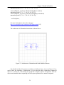
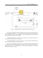
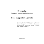
The architecture of information interactions is shown below:
Figure 5.3: Architecture of obtained model with Modelica libraries
One should consider all connectors used above as bidirected ones. Arrows in Figure 5.3 are
used to show the semantics of interactions. It’s clear that the whole construction considered
above is a virtual one. Constructing the model the compiler extracts all equations from the
objects and assembles them composing the DAE system optimized for a numeric integrator.
24
Chapter 5. Model in Modelica
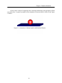
A basic feature is that all components have animation information with appropriate default
sizes and colors. A typical screenshot of the animation of beam and ball is shown in the Figure
5.4 below.
Figure 5.4: Animation of obtained model with Modelica libraries
25
Chapter 6
Control Design and Simulations
This chapter details the control design of the two obtained models with the Modelica
language. With the Newton’s second law model, we do the study through an observer design and
with the Lagrangian model we work with a linearized model and an observer to do the study. In
this chapter are also shown the obtained simulations in Simulink.
6.1
Control design
6.1.1
Control design through observer
All states are not available for feedback in many cases and one needs to estimate
unavailable state variables. Estimation of unmeasurable state variables is commonly called
observation. A device (or a computer program) that estimates or observes the state is called a
state-observer or simply an observer. If the state-observer observes all state variables of the
system regardless of whether some state variables are available for direct measurement, it is
called a full-order state observer.
An observer that estimates less than the dimension of the state-vector is called a reduced-order
state-observer or simply a reduced-order observer.
The reason for introducing the observer is that pole placement with full state feedback, is
not very practical. First, for an n-dimensional system, it requires n measurements, which, in turn,
means n transducers. Such a controller would be both expensive and bulky. Further, to be
implementable all the states would have to be measurable. Even if such a state model
formulation could be obtained, it might not be a preferred formulation.
26
Chapter 6: Control Design and Simulations
Basically, there are two forms of the implementation of an estimator as open loop and
closed-loop. The difference between these two is a correction term, involving the estimation
error, used to adjust the response of the estimator. A closed-loop estimator is referred to as an
observer.
Because of our Ball and Beam model is open loop unstable, is necessary to have some kind
of measurement of the ball velocity. The classical proportional PD-controller gets a velocity
measure by differentiating the ball position. The classical phase lead compensator does
something very similar. Another way of doing this is to use an observer based upon a model of
the ball and beam to estimate the systems states, and use the state estimates (of ball position and
velocity) in a state feedback controller.
We design a full-order state observer to estimate those states that are not measurable. We
want to do our observer as fast as it is possible, without amplifying too much high frequency
disturbances. Therefore we place the poles of the observer in the range of two to five times larger
in magnitude than the controller poles.
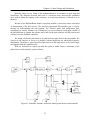
With our controller we want to get that the system is stable. Below a schematic of our
plant-observer and controller system is shown.
Figure 6.1: Simulink: Newton's second law model; plant-observer and controller
27
Chapter 6: Control Design and Simulations
6.1.2
Control Design: nonlinear system
Considering the obtained equations of motion in section 4.1.2, we do a study of control
design through a linearized state model of the system around a equilibrium position. We also
obtain a stabilizing controller for the linear model, when the angular position is measured.
The equations of motion were:
( I b + ms ⋅ rb2 ) ⋅θ&&b + 2 ⋅ ms ⋅ rb ⋅ r&b ⋅θ&b + ms ⋅ g ⋅ rb ⋅ cosθ b = τ
5
&r&b + ⋅ ( g ⋅ sin θ b − rb ⋅θ&b2 ) = 0
7
The nonlinear states are: θb, θ&b , r and r&
and the state equations become:
⎧ dθ &
⎪ dt = θ = f1
⎪
⎛ ms ⋅ g ⋅ rb ⋅ cosθ b ⎞ ⎛
⎞
1
⎪ dθ& && ⎛ 2 ⋅ ms ⋅ rb ⎞ &
⎪⎪ dt = θ = −⎜⎜ I + m ⋅ r 2 ⎟⎟ ⋅θ ⋅ r&b − ⎜⎜ I + m ⋅ r 2 ⎟⎟ + ⎜⎜ I + m ⋅ r 2 ⎟⎟ ⋅τ = f 2
s
b ⎠
b
s
b
s
b ⎠
⎝ b
⎝
⎠ ⎝ b
⎨
⎪ dr &
⎪ dt = r = f 3
⎪
⎪ dr& = &r& = 5 ⋅ r ⋅θ& 2 − 5 ⋅ g ⋅ sin θ = f
b
b
b
4
7
7
⎩⎪ dt
To have a desired equilibrium in:
θe = 0
θ&e = 0
re = 1
r&e = 0
we thus define the states a,
x1 = θ − θ e = θ
x2 = θ& − θ&e = θ&
x3 = r − re = r − 1
x4 = r& − r&e = r&
28
Chapter 6: Control Design and Simulations
and the control input,
u = τ −τ e
By substituting values in f2, we obtain:
τ e = ms ⋅ g ⋅ re
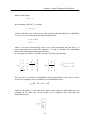
working with these new values in the state equations and considering the equilibrium,
x1=x2=x3=x4=u=0, we thus have the linearized state model:
x& = A ⋅ x + B ⋅ u
y =C⋅x
where x is a vector representing the state, u is a scalar representing the input and y is a
scalar representing the output. The matrices A, B and C determine the relationships
between the state and input and output variables.
In our system the matrices A, B and C have the following representation:
1
⎡ 0
⎢
0
⎢ 0
A=⎢
0
⎢ 0
−
5
⎢ ⋅g 0
⎣⎢ 7
0
− ms ⋅ g
I b + ms
0
0
0⎤
⎥
0⎥
⎥
1⎥
0⎥
⎦⎥
⎡
⎢
⎢
B = ⎢ Ib
⎢
⎢⎣
0 ⎤
1 ⎥
+ ms ⎥
⎥
0 ⎥
0 ⎥⎦
⎡1 0 0 0 ⎤
C=⎢
⎥
⎣0 0 1 0⎦
The next step is to check the controllability and the observability of the system. For the
system to be completely state controllable, the controllability matrix
[
Qc = B
AB
A2 B
A3 B
]
must have the rank of 4. The rank of the matrix is the number of independent rows (or
columns). In the same way, for the system to be completely state observable, the
observability matrix
⎡ C ⎤
⎢ CA ⎥
Qo = ⎢ 2 ⎥
⎢CA ⎥
⎢ 3⎥
⎣CA ⎦
29
Chapter 6: Control Design and Simulations
must also have rank of 4.
To obtain a stabilizing controller for the linearized model, we need to have a stable
characteristic polynomial for the closed loop system (roots strictly in the left half-plane). In
this example we determine a state-feedback gain (k) such that the closed-loop poles are at
s=-1 (order 4). The characteristic polynomial is:
αc(s)=(s+1)4=s4+4s3+6s2+4s+1
αc(A)=A4+4A3+6A2+4A+I
Thus, by Ackermann´s formula,
k = [0 0 0 1] ⋅ Qc−1 ⋅ α c ( A)
where, Qc is the controllability matrix previously defined.
We place the poles of the observer in s=-5, that is five time bigger than our controller
poles, with it we get that our system is faster. Thus, we have:
αo(s)=(s+5)4=s4+20s3+150s2+500s+625
αo(A)=A4+20A3+150A2+5004A+625I
Thus, by Ackermann´s formula,
⎡0 ⎤
⎢ ⎥
−1 ⎢0⎥
L = α o ( A) ⋅ Qo ⋅
⎢0 ⎥
⎢ ⎥
⎣1 ⎦
where, Qo is the observability matrix defined before.
Thus, we have the observer feedback controller,
dxˆ
= ( A − B ⋅ k − L ⋅ C ) ⋅ xˆ + L ⋅ y
dt
u = − k ⋅ xˆ
30
Chapter 6: Control Design and Simulations
The following Simulink model can be used to simulate the system.
Figure 6.2: Controller of linearized Lagrangian model in Simulink
6.2 Simulations
6.2.1 Simulations in Simulink
Simulink is an interactive environment integrated in Matlab for modeling, simulation and
analyzing dynamic systems. Simulink provides a graphical user interface for constructing block
diagram models via drag and drop operations. Models can be grouped into hierarchies to create a
simplified view of components or subsystems. Therefore a model built up in Simulink consists of
blocks that correspond to subsystems of the model. In each block there are mathematical
relationships that describe the physical behavior of the system. If the subsystems affect each
other, information between the blocks has to be exchanged in order to evaluate the relationships.
The benefit with Simulink is the easy to use design and since the software is integrated
with Matlab it makes it very powerful with a lot of useful analysis and design applications.
31
Chapter 6: Control Design and Simulations
Another benefit is the easy way to create plots of signals. Further, the ability to easily and
quickly simulate a model built in Simulink is another benefit with this modeling program.
However it lacks the benefits of Modelica to define implicit equations and relationships.
¾ Control design through observer
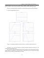
Figure 6.3: Simulations obtained with the Newton’s second law model and observer
In Figure 6.3 we can see the behavior with the calculated controller and observer. The
closed loop system behaves well.
We can observer how the position and the position estimate of the ball are almost the same.
Both responses are stabilized at 1 like the reference, and besides we can see that the beam angle
and the velocity estimate are stabilized in few seconds.
32
Chapter 7
Experiments
This chapter describes the experimental setup for the Ball and Beam experiments. Initial
experiments are performed to identify process parameters and finally the control experiments are
performed. An alternative implementation to the one described in Chapter 6 is presented.
7.1 Experimental Setup
We use the ball and beam process shown in Figure 7.2. The beam is controlled by a DCmotor and the beam angle can be measured. The ball position is estimated from a vision system
written by Tomas Olsson, PhD student at the Department of Automatic Control and uses a Fire-i
camera connected to a PC running a “ball detection” program. The ball coordinates are sent via a
network connection to a Linux PC running the control implementation in a real-time extension of
Matlab/Simulink developed by A.Blomdell. A sketch of the connections can be visualized in
Figure 7.1.
33
Chapter 7. Experiments
Vision @Windows PC
Fire-i
matcomm
Simulink ctrl@Linux PC
Figure 7.1: Sketch of the connections between used ball and beam, vision system and PC’s
7.2 How to do the experiments
The first task in this work consists of determining which is the correct model of the real
process of the ball and beam, including finding appropriate parameters. To find this correct
model, we do some experiments with the real process. The “ball and beam”-process is shown
below and the controller is implemented in Matlab/Simulink with a real-time extension, where a
Simulink block represents the connection to analog inputs and analog outputs, see Figs. 7.2 and
7.3.
Figure 7.2: Ball and Beam used
34
Chapter 7. Experiments
Figure 7.3: Controller of the Ball and Beam process
Beam-angle dynamics
The beam is directly connected to a DC-motor without any gearbox according to Fig. 7.4.
Here we can note that there is a distance, d, between the motor axis and the beam. This will make
the beam oscillate like a pendulum if no control signal, u, to the motor, is applied, and thus we
can expect an oscillatory behavior. We will first do a simple experiment to find out the
eigenfrequency and possible damping of this motion. The next step is to find the gain from
commanded control signal in the Simulink model to the motor torque and to the process output
(beam angle).
Figure 7.4: Ball and beam with distance d
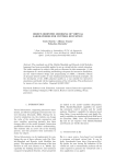
We first start with applying an impulse disturbance to the uncontrolled beam for an initial
angle=0. The input signal proportional to the beam angle is shown in Fig.7.5.
Figure 7.5: Response of the beam with applied impulse
35
Chapter 7. Experiments
The period time of the oscillation is approximately 3 seconds, therefore the frequency
w ≈ 2rad/s. Now that we have our frequency, we can find which are our damping and our
overshoot.
With these values and using tools of Matlab we can observer the impulse response of the
system being this shown in the Fig 7.6:
Figure 7.6: Impulse Response of the Ball and Beam process
We can observer from the response, that there is an additional damping and an oscillatory
behavior, in comparison what we have discussed previously.
From Figure 7.6, we can estimate the impulse response correspond to a system, which
transfer function has a gain ≈ 22. This gain has been calculated through of the Figure 7.5.
G=
22
s + 0.6 ⋅ s + 4
2
Through this transfer function, we can represent the system in state-space form, doing it
the following way:
u
y
22
s 2 + 0 .6 ⋅ s + 4
s 2 ⋅ y + 0.6 ⋅ s ⋅ y + 4 ⋅ y = 22 ⋅ u
36
Chapter 7. Experiments
we have x1=y, then the state equations are:
x&1 = x2
x& 2 = &y&
substituting:
x& 2 = &y& = −0.6 ⋅ y& − 4 ⋅ y + 22 ⋅ u
x& 2 = −0.6 ⋅ x 2 − 4 ⋅ x1 + 22 ⋅ u
The state-space representation is shown below:
⎧⎡ x&1 ⎤ ⎡ 0
1 ⎤ ⎡ x1 ⎤ ⎡0 ⎤
⎪⎢ ⎥ = ⎢
⎥ ⋅ ⎢ x ⎥ + ⎢22⎥ ⋅ u
&
4
0
.
6
−
−
x
⎣
⎦ ⎣ 2⎦ ⎣ ⎦
⎪⎣ 2 ⎦
⎨
⎪ y = [1 0]⋅ ⎡ x1 ⎤
⎢x ⎥
⎪
⎣ 2⎦
⎩
(7.1)
To do the study of the system we write an m-file in Matlab. In this m-file we include the
matrices of state-space system and the obtained values of desired frequency and damping. With
these values we can calculate the desired roots of our system.
Now we have our poles, we can use Matlab to find a controller (k matrix) by using the
place command, see Chapter 6.
To implement our controller we have to find an observer, which can do an estimation of
the unmeasurable state variables. Normally the poles of the observer are faster than those of the
controller. We place the poles two times faster than our controller. The observer is basically a
copy of the plant; it has the same input and almost the same differential equation. An extra term
compares the actual measured output y to the estimated output ŷ ; this will cause the estimated
states x̂ to approach the values of the actual states x. The error dynamics of the observer are
given by the poles of (A-L*C). In the same way as before with the command place we find the
observer (L matrix).
The next step is to do the Simulink model with the plant of the real process and the
obtained observer and controller. This Simulink model is shown in the Fig 7.7.
37
Chapter 7. Experiments
Figure 7.7: Simulink model of observer based control of beam angle
We can now simulate the closed-loop response and we can check if the found model is
correct. Changing the values the w we can observer if the system is faster or slower and we can
see if its behavior is right. We can also change the values of the inputs the check if the response
of the real process is correct in every moment.
A design problem does not necessarily have a unique answer. Using this method (or any
other) may result in many different compensators.
For the implementation to control the real process we use a discrete-time feedback from an
observer based on a sampled version of the system 7.1.
We have used the Matlab command c2d to convert between continuous and discrete time.
The sampling time for the Simulink controller was set to 10ms. The poles of the discrete-time
design (used in place) was transformed from continuous-time specifications according to
disc_pole=exp(cont_pole.* tsamp).
38
Chapter 7. Experiments
Ball controller
For the real-time implementation of the ball controller we have chosen to do a cascadedesign, re-using the beam-controller from the previous subsection for the inner loop, instead of
the controlled presented in Chapter 6.
The coordinates of the ball from the vision systems are updated with 30Hz. However the
camera pictures may be delayed ≥ 30ms in the controller and the camera is not synchronized
with the rest of the controller. To handle this uncertainty we have chosen to run a faster inner
loop and an outer-loop with a slower sampling rate.
From Chapter 4, we have an approximate model of a double integrator from beam angle to
ball position, and we start to do a simple experiment to find out the gain with respect to the
position provided by the vision system. We can visualize it in the figure 7.8.
Figure 7.8: Graphic to find out the gain with respect to the position provided by the vision system
A video sequence of the experiment can be found at [13].
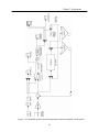
39
Chapter 7. Experiments
Figure 7.9: Simulink model to do the beam control
40
Chapter 7. Experiments
Figure 7.10: Simulink model to do the ball position controls trough the vision system
41
Chapter 8
Conclusions
In this chapter the conclusions of this work are presented followed by suggestions on how
to continue the development.
8.1 Conclusions
The main goal of this thesis was to do the modeling and control of the Ball and Beam
process. This objective has been fulfilled by the presentation of several kinds of control, which
have been done through Modelica and Matlab and finally by experiment on the real process.
Over this thesis we can visualize how control theory relates to real systems. Computer
simulations can help, but simulations alone are limited by how well the system in question has
been modeled. It is more enlightening if the results obtained theoretically are actually applied to
a physical system. Applying the theoretically calculated results to a real system helps us not only
visualize, but to evaluate how well the model was able to predict the system performance.
The best way to learn about control systems is to design a controller, apply it to the system
and then watch the system in operation. A system is modeled on a computer, and, with the help
graphics, the system can be seen in action. However, the system being observed in the simulation
is in reality just a model of the true system. The model must always be a simplified
representation of the system, and cannot reproduce all aspects of system behavior. Such effects
are difficult to simulate, and are best understood from hands-on experience with the physical
system.
42
List of Figures
Chapter 2
Figure 2.1: Motor drive with Modelica libraries .................................................................... 6
Chapter 3
Figure 3.1: Diagram of Ball and Beam ................................................................................... 9
Figure 3.2: Ball and Beam connected via gearbox .............................................................. 10
Figure 3.3: Ball and Beam directly connected to the axis of a DC-motor............................. 11
Chapter 5
Figure 5.1: Dymola simulation: Response of beam angle, position of the ball and
velocity open-loop response for model base on Newton’s second law ................................ 21
Figure 5.2: Dymola simulation: Response of beam angle, position of the ball and
velocity Open loop response for the Lagrangian model ....................................................... 22
Figure 5.3: Architecture of obtained model with Modelica libraries .................................... 24
Figure 5.4: Animation of obtained model with Modelica libraries ...................................... 25
Chapter 6
Figure 6.1: Simulink: Newton's second law model; plant-observer and controller............... 27
Figure 6.2: Controller of linear Lagrangian model in Simulink ............................................ 31
Figure 6.3: Simulations obtained with the Newton’s second law model and observer ......... 32
Chapter 7
Figure 7.1: Sketch of the connections between used ball and beam, vision system and
PC’s........................................................................................................................................ 34
Figure 7.2: Ball and Beam used ............................................................................................ 34
Figure 7.3: Controller of the Ball and Beam process ............................................................ 35
Figure 7.4: Ball and beam with distanced ............................................................................. 35
Figure 7.5: Response of the beam with applied impulse ...................................................... 35
Figure 7.6: Impulse Response of the Ball and Beam process ............................................... 36
Figure 7.7: Simulink model of observer based control of beam angle ................................. 38
Figure 7.8: Graphic to find out the gain with respect to the position provided by the
vision system ......................................................................................................................... 39
Figure 7.9: Simulink model to do the beam control ............................................................. 40
Figure 7.10: Simulink model to do the ball position controls trough the vision system ...... 41
Bibliography
[1]
Hilding Elmqvist, Dag Brück, Sven Erik Mattsson, Hans Olsson and Martin Otter,
Dymola Dynamic Modelling Laboratory User's Manual, version 5, Sep2002
[2] Dynasim AB
Research Park Ideon
http://www.Dynasim.se
SE-22370 Lund SWEDEN
[3] Modelica Homepage:
http://www.modelica.org
[4] Dymola Homepage:
http://www.dymola.com
[5] Modelica Association (2002):
"Modelica - A Unified Object-Orientec Language for Physical Systems
Modeling", Language Specification, Version 2.0, 30 January 2002.
[6] Michael Tiller, Introduction Physical Modeling with Modelica, 2001
Kluwer Academic Publishers, Boston ISBN 0-7923-7367-7
[7] Beginner tutorial:
http://www.modelica.org/Conference2002/BeginnersTutorial.zip
[8] Modelica documents:
http://www.modelica.org/documents.shtml
[9] Advanced tutorial:
http://www.modelica.org/Conference2002/AdvancedTutorial.zip
[10]
Master Thesis Project:
Xavier Callier. Department of Automatic Control. Lund Institute of Technology.
August 2002 – January 2003
[11]
Master Thesis Project:
Francesco Calugi. Department of Automatic Control. Lund Institute of
Technology. October 2001 – April 2002
[12]
http://www.modelica.org/Conference2003/papers.shtml
Session 8A
Mechatronic Systems - II
297
Ivan I. Kossenko and Maia S. Stavrovskaia Moscow State University of the
Service, Russia: How One Can Simulate Dynamics of Rolling Bodies via Dymola:
Approach to Model Multibody System Dynamics Using Modelica
[13]
http://www.control.lth.se/education/masterthesis/BaB_video.npg