1
Yeast Colony Counter User Manual
Jan Schier, Bohumil Kovář
[email protected], +420-2-6605 2470
Department of Image Processing
http://zoi.utia.cz
Contents
1 Introduction
1.1 Image characteristics
. . . . . . . . . . . . . . . . . . . . . . . . . . . . . . . . . . . . . . .
1
1
2 Installation of the tool
1
3 Launching the tool
2
4 Home screen
4.1 First start of the tool . . . . . . . . . . . . . . . . . . . . . . . . . . . . . . . . . . . . . . . .
4.2 Subsequent run of the tool . . . . . . . . . . . . . . . . . . . . . . . . . . . . . . . . . . . . .
4.3 Selection of the result file . . . . . . . . . . . . . . . . . . . . . . . . . . . . . . . . . . . . .
2
3
3
3
5 Processing the dishes in the supervised mode
3
6 Result file – filename and format
5
7 Processing flow
5
8 Image checking
6
9 A note on the tool performance
7
10 Acknowledgements
7
© 2010, 2011 ÚTIA AV ČR, v.v.i.
All disclosure and/or reproduction rights reserved.
Revize
Revize
0
1
Datum
1.10.2010
23.02.2011
Autor
J.S.
J.S.
Popis změn v dokumentu
Vytvořenı́ dokumentu
Aktualizace pro SW verzi 22.02.2011
2/8
1
Introduction
This document describes the use of the yeast colony counter developed in UTIA AV CR, Prague. It can
be used to process series of images of Petri dishes containing yeast colonies. It is aimed for a research
laboratory using standard imaging equipment (darkroom, general purpose camera on a stand) and hand
manipulation of the dishes rather than specialized single-purpose camera system. It is assumed that dark
background is used in the images.
The tool evaluates two figures for the images: the relative coverage of the dish, and the number of
colonies in the dish. It provides two modes of operation: automatic or semi-automatic. In the automatic
mode, it processes the batch of images without any user intervention. In the semi-automatic mode, it first
performs automated thresholding, dish localization, and a counting attempt, then it provides the user with
an editor, where he can interactively correct the result of counting.
Two image formats are accepted at this moment: j̇pg and ṫiff. Other formats may be added on request.
Note: The tool is citeware. If you find the application useful for your purpose, we will be very thankful
if you can cite our paper Schier, J., Kovář, B.: Automated counting of yeast colonies using the Fast Radial Transform algorithm, BIOSTEC 2011 4th International Joint Conference on Biomedical Engineering
Systems and Technologie, Rome, Italy, 2011, see also http://www.utia.cz/node/631/0355696.
1.1
Image characteristics
The images under consideration are characterized by the following properties:
+ typical resolution of an image is 1024×768 pixels,
+ dark background is used to increase image contrast,
+ illumination by two linear lights along the short edges,
+ colonies are roughly round-shaped,
– variations of dish position,
– varying diameter of the dish in image,
– varying intensity of the dish background.
– colonies often form clusters.
2
Installation of the tool
The tool comes in the form of a self-extracting archive, which contains the tool self (ColonyCounter.exe),
and the Matlab Compiler Runtime Installer (MCRInstaller.exe), which is necessary to run the tool. When
running the ColonyCounter pkg archive, the files are extracted into the directory of archive and the
MCRInstaller is automatically launched. It asks to choose the setup language (choose the default – “English”) and for permission to install the VCREDIST X86 (Visual C++ Redistributable) (choose “Install”).
The installation continues automatically until the MCR InstallShield Wizard asks for several installation
options: fill in the User information or just click on “Next”; select installation directory and then launch
the installation. The InstallShield may ask about installation of the .NET Framework - just click “OK” to
continue.
When the installation process is finished, the ColonyCounter.exe program is unpacked to the directory.
This is the tool self — other files can be safely removed.
1/8
3
Launching the tool
To launch the tool, simply run the ColonyCounter executable, e.g. with Start→Run→ColonyCounter. The
start of the program takes some 15 s on our system.
4
Home screen
After launching the tool, the home screen appears, as shown in Figure 1. It is used to select the following:
Figure 1: Home screen of the tool
• Image directory: directory with the images to process (directory tree is possible as well)
• Result directory: location and file name for the file containing the results of processing
• Mode: either Supervised — with graphical editor for correction of the colony detection results, or
Batch — fully automatic.
• Start processing: is used to start the processing, after making the necessary selections.
2/8
4.1
First start of the tool
On the first start of the tool, the Result directory and Start processing items are disabled. The user is
forced to make the selection of the image directory, after which the Result directory item will be enabled.
Finally, after having selected the result file, the Start processing item will also get enabled.
Note: the values of the image directory and result file selections are stored in the ColCounterConfig.txt
file between the runs of the tool.
4.2
Subsequent run of the tool
On the subsequent runs of the tool, the values of the image directory and result file from the last run
are re-loaded. The Start processing item is now enabled on the tool launch. If the image directory is
changes, warning about the change is issued, reminding the user to check the location of the result file
(see Figure 2), and the Start processing button gets disabled.
Figure 2: Warning message after directory change
4.3
Selection of the result file
The default mode, which is used if the user does not make any selection on a subsequent run of the
tool (neither image directory nor result file), is to continue the processing of the given image directory
and to append to the result file. The tool goes through the result file, checks the results against the files
in the directory tree, deletes the data for the images that are not present any more, and continues with
processing at the point where is has been interrupted on the last run.
If the user decides to open the Result file selection window, and selects the same file, he gets a series
of warning dialogues:
• First warning about overwriting the file comes from MSWindows and could not be eliminated. Nevertheless, the user will have chance to choose to append or overwrite the results file in the following
dialogue windows, so it is safe to choose to overwrite at this point.
• The warning that is issued next, is shown in Figure 3. Here, user is offered the possibility either to
Append (default) or to Overwrite the result file.
• If he selects to overwrite the file, he is warned once more, as shown in Figure 4, with the default
selection set to No (that is, do not overwrite the results). Selecting Yes in this dialogue will result in
overwriting the results.
5
Processing the dishes in the supervised mode
In the supervised mode, the results of processing (the detected colonies) are presented in an editor
window, as shown in Figure 5. This window has several function and information areas:
3/8
Figure 3: Warning dialogue: existing result file
Figure 4: Overwrite conformation dialogue
Figure 5: Dish editor window
• Window title: path and filename of the image
• Top area: results: relative area and number of colonies
• Central area: image of the dish with colonies, with marks on detected colonies
• Bottom part: Buttons Delete marks, Add marks and Zoom, used to correct the counting result and
4/8
the button Next dish.
The meaning of Delete and Add is obvious. Zoom button switches to zoom mode, which can be
used to zoom-in an area-of-interest in the dish. Both click-hold-drag and scroll-wheel can be used.
Next dish is used to finish processing of the given dish and to proceed to the next one.
• Right column: Stop button can be used to interrupt processing. Save image can be used to save
image of the dish with detection signs for archival purposes.
Note: the filename of the saved images is, by default, given an appendix saved. The user can
choose any filename and location; however, the images with this suffix, if present in the image
directory, are ignored by the tool when it seeks for the images to process (obviously, processing
screenshots would give little sense).
6
Result file – filename and format
The file with results is stored in the CSV (Comma-Separated Values) format, which can be loaded into
MS Excel, OpenOffice Calc, and probably other spreadsheet programs as well. The values are separated
by semicolon.
The default name of this file, as suggested by the tool, is the name of the root directory of the image
tree with the results suffix, e.g. images results.csv. However, any filename can be selected by user.
A line in the file has the following structure:
1. path to the image from the root of the image directory tree (e.g. images/dense/1.jpg). Note: this
is the same value as displayed in the title-bar of the image editor (Section 5).
2. relative coverage of the dish in percents
3. number of colonies in the dish
The result file is updated immediately after processing each dish, so it is save to interrupt the processing.
7
Processing flow
Processing flow of the tool is outlined in Figure 6.
First step of the processing includes thresholding of the image and localization of the dish — let us
recall that the dishes are hand manipulated (Sec. 1), hence, the position if the dish in each image is
slightly different. In this step, the image is also checked for correctness.
The thresholding is used to separate the dish from the background and to perform image segmentation, that is, to extract the (clusters of) blobs. To determine the threshold for separation of the dish from
the background, samples of background from the image corners are used. To determine threshold for the
blobs extraction, Otsu method is used.
Next step is resolution of the clustered blobs: the Fast Radial Transform [Loy and Zelinsky, 2003]
is used to construct symmetry map of the objects in the image. Then, the nonmaxsuppts function
[Kovesi, 2005] is used to find local maxima of this map, which represent the centers of the colonies.
Finally, the position of the centers if checked to filter out cases which would be obviously wrong (e.g.
colony center falling in the background).
5/8
Input:
Set of images
Preprocessing:
Thresholding
Dish locating
Image segmentation
Resolution of
clustered colonies:
Blob center
location map
Blob center
determination
Figure 6: Processing flow of the colony counter
8
Image checking
In the first step, image is also checked for correctness, to ensure sufficient robustness of the processing.
This check involves mainly the position and size of the dish: it should be roughly centered and the
inner part (that is, the part with the grow medium) must be completely present in the image, so that the
coverage is evaluated correctly.
The image of the dish must be also sufficiently large, to provide reasonable accuracy of detection.
Currently, the setting is that the dish must occupy at least 50% of the image height.
The background distortions, such as that shown in Figure 7, are eliminated in the process of dish
location and background masking, as long as the distortion does not overlap with the dish in vertical
projection.
Figure 7: Example of background error
6/8
9
A note on the tool performance
The performance of the tool has been tested using 245 images of Petri dishes, containing mostly less
than 60 colonies per dish. The performance is summarized in Table 1. More details are given in
] colonies
0 – 17
18 – 20
21 – 23
24 – 26
27 – 29
30 – 40
41 – 49
50 – 60
> 60
samples
21
19
25
29
27
35
30
29
30
missed [%]
1.47
2.99
3.31
4.00
3.28
4.17
4.00
3.87
5.36
false [%]
0
0
0
0
0
0
0
2.00
3.22
Table 1: Dependence of the counting errors on the number of colonies in the dish. The system average
counting error is under 4%
[Schier and Kovář, 2011a] and [Schier and Kovář, 2011b].
10
Acknowledgements
The images included in the package have been prepared in the Department of Genetics and Microbiology,
Faculty of Natural Sciences, Charles University. The software has been developed in cooperation with
this laboratory.
The development of the tool has been supported from the Ministry of Education, Youth and Sports
project 1M0567 and from the project TA01010931 of the Technology Agency of the Czech Republic.
7/8
References
[Kovesi, 2005] Kovesi, P. D. (2005). MATLAB and Octave functions for computer vision and image processing. School of Computer Science & Software Engineering, The University of Western Australia.
Available from: http://www.csse.uwa.edu.au/∼pk/research/ matlabfns/.
[Loy and Zelinsky, 2003] Loy, G. and Zelinsky, A. (2003). Fast radial symmetry for detecting points of
interest. IEEE Transactions on Pattern Analysis and Machine Intelligence, 8(25):959–973.
[Schier and Kovář, 2011a] Schier, J. and Kovář, B. (2011a). Automated counting of yeast colonies using
the fast radial transform algorithm. In Pellegrini, M., Fred, A., Filipe, J., and Gamboa, H., editors, BIOINFORMATICS 2011, Proceedings of the International Conference on Bioinformatics Models, Methods
and Algorithms, pages 22–27, Rome, Italy. INSTICC, SciTePress.
[Schier and Kovář, 2011b] Schier, J. and Kovář, B. (2011b). A semi-automatic software tool for batch
processing of yeast colony images. In Zhang, J. J., editor, Proceedings of the IASTED International
Conference Signal Processing, Pattern Recognition, and Applications (SPPRA 2011), volume 721SPPRA, pages 206–212, Innsbruck, Austria. IASTED, ACTA Press.
8/8