Download Physical characterization of the frozen fragments of the Tagish Lake

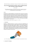
Physical characterization of the frozen fragments of
the Tagish Lake meteorite
by
Maxim Ralchenko
A thesis submitted to the Faculty of Science in partial fulfillment of the requirements
for the degree of Bachelor of Science
Department of Earth Sciences
Carleton University
Ottawa, Ontario
August 2013
The undersigned recommend to the Faculty of Science acceptance of this thesis
Physical characterization of the frozen fragments of
the Tagish Lake meteorite
submitted by Maxim Ralchenko in partial fulfillment of the requirements of the
degree of Bachelor of Science.
______________________________
Dr. Claire Samson, Thesis Supervisor
Professor
Department of Earth Sciences
Carleton University
______________________________
Dr. Richard Herd, Thesis Supervisor
Natural Resources Canada
Adjunct Professor
Department of Earth Sciences
Carleton University
______________________________
Dr. Sharon Carr
Chair, Department of Earth Sciences
Carleton University
iii
Abstract
The Tagish Lake meteorite is a C2 ungrouped carbonaceous chondrite with
unique physical and chemical properties. There are two groups of fragments: pristine,
which are those recovered within days of the 18 January 2000 fall, and degraded,
recovered a few months later in the spring.
The objective of this study was to non-destructively characterize the physical
properties of Tagish Lake, specifically by measuring bulk density and porosity for a
suite of pristine fragments. The bulk density was measured via laser imaging and
porosity was measured via helium pycnometry. Laser imaging has been previously
successfully used to characterize a variety of stony and iron meteorites. However, due
to the uniqueness and fragility of this meteorite—both chemically and physically—it
is kept permanently in a freezer at temperatures never exceeding -10°C.
The laser camera used in this study, the Konica Minolta Vivid-9i, is not
designed to be used at -10°C. To protect it against the cold, a method of wrapping it
with thermal blankets was devised. These measures allowed the camera to be
operated for at least two hours in the cold consecutively, after which it had to be taken
outside the cold room to be warmed up. Through this work, it was shown that the
laser camera could be adapted for use in an extreme environment, which will allow it
to be used in the future to characterize other frozen artifacts or geological materials.
The bulk density of the 13 measured Tagish Lake fragments mostly clustered
around 1.80 g/cm³, with some near 1.90 g/cm³, possibly because of differences in
lithology. The measured porosity for 11 fragments was generally near 30%, with
some deviation accounted for by lithology or contamination. Compared to previously
published literature values, which are mostly for degraded fragments, the measured
bulk density was higher, and the porosity was lower. As fragment degradation
involves the loss of volatiles, this result is not surprising. However, Tagish Lake is
quite hydrophilic, which may complicate the comparison between different suites of
data.
This study was part of a systematic analysis of the meteorite, and this bulk
density and porosity data will be integrated with other studies in the future.
iv
Acknowledgements
I first thank my co-supervisors, Dr. Claire Samson and Dr. Richard Herd, for all of
their guidance and advice during this project.
Dr. Dan Britt of the University of Central Florida provided financial support, traveled
with, and operated his helium pycnometer in Edmonton, and gave insight into the
interpretation of the data.
Dr. Christopher Herd of the University of Alberta welcomed me and Dr. Britt into his
lab to access samples and was an immense source of knowledge about the meteorite.
Dr. Jason Mah laid the groundwork for the thermal protection of the camera.
Po Kong Lai lent his laptop, capable of receiving data from the laser camera, for use
during the tests in Ottawa and for the trip to Edmonton.
Penka Matanska and Mike Antunes of the Department of Physics lent thermocouples
and multimeters for use with the laser camera and gave excellent advice which
greatly improved the design of the thermal protection.
Dr. Tim Patterson and his lab members gave me access to their cold room so that I
could test the camera in the cold prior to going to Edmonton. Their patience with me
over several weeks, as I occupied a considerable portion of their lab space, and sat in
the cold room containing over half a million dollars worth of geological samples, is
very much appreciated.
Beth Halfkenny lent me a suite of coal samples to use as analogues to Tagish Lake
while I was experimenting in Ottawa.
Dr. Phil McCausland at Western University provided valuable insight into the nature
of the Tagish Lake meteorite.
Last but not least, Chris Fry has shared his invaluable expertise with laser imaging
and modeling since last year.
v
Table of contents
Title page
ii
Faculty approval page
iii
Abstract
iv
Acknowledgements
v
Table of contents
vi
List of tables
viii
List of figures
ix
1. Introduction
1
Research objectives
1
Importance of bulk density and porosity
2
Tagish Lake meteorite background
2
2. Methods
10
Definitions of bulk density and porosity
10
Measurement of density
11
Measurement of porosity
16
3. Thermal stability
19
Background
19
Dewpoint
19
Camera
23
Design of protection against the cold
24
Test results
28
Conclusion and addendum
34
4. Results
37
Error analysis
40
5. Discussion
45
6. Conclusions and future work
55
7. References
58
Appendix A: Test plans
61
Part A – Camera tests at Carleton
62
vi
7
Preamble
Equipment list
62
66
Test 1: Unplugged cooling and warming test
67
Test 2: Plugged-in cooling and warming test
69
Test 3: Covered cooling and warming test
71
Test 4: PCA tests
75
Test 5: Analogue tests
77
Part B: Scanning of meteorite samples at Edmonton
79
Preamble
79
Description
79
Appendix I
81
Appendix II
82
Appendix III
85
Appendix B: Raw data outputs
86
Appendix C: Raw scan and model data
87
List of tables
Table 1: Density and porosity values for Tagish Lake from previous studies
Table 2: Bulk density and porosity of 13 pristine Tagish Lake fragments
viii
8
38
List of figures
Figure 1: Photograph of manual turntable used to orient meteorite samples
12
Figure 2: Photograph of cold room set-up for laser imaging
15
Figure 3: Photograph of pycnometry set-up
18
Figure 4: Psychometric chart used to calculate dewpoint
22
Figure 5: Annotated diagram of laser camera
26
Figure 6: Photograph of preparation of camera for the cold room
27
Figure 7: Photograph of the working design for thermal protection of the camera
30
Figure 8: Graph of camera temperature with time during a cold room test
31
Figure 9: Graph of test results for optical stability with time
33
Figure 10: Graph of porosity and bulk density for Tagish Lake fragments
39
Figure 11: Graph of test results for optical stability at Edmonton
41
Figure 12: Graph of model standard deviation as a function of bulk volume
43
Figure 13: Graph comparing literature and measured values
47
Figure 14: Model of fragment P-10a with broken surface centred
48
Figure 15: Photograph of P-10a with similar orientation to that in Figure 14
49
Figure 16: Model of fragment P-10a with fusion crust centred
50
Figure 17: Photograph of P-10a with similar orientation to that in Figure 16
51
Figure 18: Model of fragment P-4 with unusual surface visible
52
ix
1. Introduction
Research objectives
The main objective of my research was to enrich the database of values for
bulk density and porosity for pristine samples of the Tagish Lake meteorite held in the
Meteorite Collection of the University of Alberta. These physical parameters were to
be analyzed in detail as they yield clues to the character of the processes that have
formed and evolved the meteorite and its parent body. Some fragments of the Tagish
Lake meteorite are termed pristine because they are frozen. Specifically, it means that
they were recovered within days after the fall (18 January 2000) and kept at a cold
temperature since then; between the fall and their arrival at the University of Alberta,
they were not allowed to warm up above -7°C. The key characteristic that qualifies a
sample as pristine or not is the presence of certain volatile organic compounds (e.g
naphthalene): if they are present, the sample is pristine, otherwise it has thawed (Herd
R.K., 2013). A helium pycnometer was used to determine porosity; the instrument
was brought to Edmonton by Dr. Dan Britt of the University of Central Florida. Bulk
density was determined by 3D laser imaging, and the Konica Minolta Vivid 9i 3D
digitizer1 used in that step was transported by me. These 3D models are now excellent
archives of the pristine fragments. Destructive sampling is eventually unavoidable for
a portion of the fragments due to the unique organic chemistry of the meteorite.
Finally, a major part of the project became to design a way by which the laser camera
could operate in the cold room in which the meteorite is studied. The electronics are
of commercial grade and are not reliable below +10°C, whereas the cold room in
which the work took place was at -10°C.
1
Also referred to as simply “digitizer”, “laser camera”, or “camera”.
2
Importance of bulk density and porosity
Bulk density and porosity are intrinsic physical properties that provide insight
into the processes that have formed and evolved a meteorite and its parent body (Britt
and Consolmagno, 2003; Consolmagno and Britt, 1998; Consolmagno et al., 2008).
Bulk density can be used to help classify meteorites, and is required in the
determination of porosity. Questions that are posed in regards to porosity often centre
around its cause. What causes some meteorites to lithify and compact more than
others? Carbonaceous chondrites—the category into which the Tagish Lake meteorite
is classified—have a characteristically high porosity of over 20%. This observation
suggests that this category of meteorites formed under physical processes that are
much different than for other meteorites. Tagish Lake, being very friable and fragile,
is an extreme case. Density and porosity must be considered at all possible scales,
from micrometeorites to the parent body. It is also a useful exercise to relate these
physical properties of meteorites to their parent body asteroids; however, meteorites
may not necessarily be representative samples, as they are either strong material (that
has survived passage through Earth's atmosphere) or weak material (that was weak
enough to have been ejected from its parent) (Consolmagno et al., 2008). Finally, as
will be most applicable during this study, trends in bulk density and porosity for a
meteorite with several fragments—this is the case with Tagish Lake—are considered
as well. On a first-order basis, the trends tell us if the meteorite is homogeneous or
heterogeneous.
Tagish Lake meteorite background
The Tagish Lake meteorite is an ungrouped type 2 carbonaceous chondrite
with unique physical and chemical properties. The meteorite, which fell on Tagish
3
Lake in northern British Columbia near the border with the Yukon on January 18,
2000, has not yet been extensively characterized with regards to its physical
properties.
The circumstances regarding this fall are particularly fortuitous. The Tagish
Lake meteorite, hereafter to referred to as “Tagish Lake”, is very friable and overall
mechanically weak. The meteorite is one of a kind; as stated by Brown et al. (2002),
“Tagish Lake does not seem to fit into our existing meteorite taxonomy, having
characteristics that set it apart from any other meteorite.” This uniqueness of the
meteorite is at least partially an artifact of it being unstable at the Earth's surface.
The meteorite was recovered in two expeditions. The first fragments,
recovered within several days after the fall, are termed pristine, as they not have been
thawed (Hildebrand et al., 2006). There was originally under 900 g of pristine
material available prior to destructive sampling. When the material was acquired by
the University of Alberta-led consortium, approximately 200 g was given to the
Royal Ontario Museum, and approximately 650 g to the University of Alberta
Meteorite Collection. Prior to the acquisition, over 40 g of material was consumed
for, e.g., organic studies on the 10.39 g fragment 8a, chipping off parts of fragments 1
and 2, and the creation of thin sections (Herd R.K., 2013). Approximately 26 g of
material has been consumed in organic studies after the acquisition (Herd C.D.K.,
2013b; Herd et al., 2011a). Overall, about 620 g of pristine material remains at the
University of Alberta. These pristine samples were collected by local resident Jim
Brook, who took care to avoid touching the fragments with his bare hands.
Shortly after the fall of Tagish Lake, a large snowstorm interrupted further
4
recovery efforts, and a second expedition was mounted a few months later in the
spring (late April to early May) to recover more fragments. These samples are termed
degraded, as they have either been warmed up or in contact with water. The instability
of the meteorite is evident: it turns into mud when in contact with water and emits a
sulfurous smell. The dust cloud which formed when the meteorite broke up in the
atmosphere also had an odor associated with it, described variously as “foul, metallic,
sulfurous, or chemical” (Hildebrand et al., 2006). The original mass was in excess of
60 metric tonnes and it entered the atmosphere at a low entry angle and velocity
(entry angle of 14.5±1.6° at azimuth 330.7±2.4° traveling at 15.8±0.6 km/s); the
combination of these circumstances allowed for some fragments to survive
(Hildebrand et al., 2006). The question of whether the recovered material is
representative of the whole mass, or only the stronger fragments of a heterogeneous
body was brought up by Hildebrand et al. (2006). The conclusion that was made by
the authors is that because a range of grain densities were measured (2.56–2.91
g/cm3), the fragments constitute representative sampling of the whole body
(Hildebrand et al., 2006). The fragility and chemical instability of the meteorite
requires that it be stored in a freezer (usually set to -20°C), which incidentally makes
it a prime example of cold curation as could be needed for samples returned from
future Solar System missions (Herd et al., 2011b; Hilts et al., 2012). Mechanically,
Tagish Lake is extremely weak; while there is a range of weaker and aqueously
altered (or “dusty”) to stronger lithologies and fragments, the mere act of handling the
meteorite during imaging left dust to sand-sized bits of material on the turntable
surface. There are trends within the suite in organic matter and isotope abundances
that describe the degree of aqueous alteration (Herd et al., 2011a). These trends can
5
be extrapolated to characterize interstellar, nebular, and parent body processes (Herd
C.D.K., 2013a).
Carbonaceous chondrites are the most chemically unfractionated group of
meteorites, and are particularly rare, as they constitute around 5% of the meteorites
known. Traditionally, carbonaceous chondrites are a group of meteorites having
peculiar characteristics such high friability, generally low density, and little to no free
nickel iron (Mason, 1962). The modern definition given by the Meteoritical Society is
based on their chemistry; the oxygen isotope compositions plot below the terrestrial
fractionation line, and most of the carbonaceous chondrites have Mg/Si ratios near the
solar value. They are then further classified by petrologic type and group.
Tagish Lake was described by Hildebrand et al. (2006) as one the most
primitive meteorites known. It is ungrouped, but it has affinities to both the CI and
CM groups (Consolmagno et al., 2008); in their report documenting the fall of the
meteorite, Brown et al. (2000) described it as an intermediate specimen between the
CM and CI groups. The main affinities to the CM group are the presence of
chondrules, altered calcium-aluminium inclusions (CAIs), and the presence of
individual olivine grains. It is also has affinity to the CI group based on the bulk
chemistry, abundant magnetite, high carbon content, and extreme friability. However,
the composition of the carbonate minerals in Tagish Lake were distinct from what had
been previously observed in either the CI or CM groups (Norton, 2002). As Tagish
Lake is sufficiently distinguishable from other meteorite groups, it has been classified
as ungrouped.
Zolensky et al. (2002) classified Tagish Lake as a type II carbonaceous
6
chondrite and suggested a possible affinity to the CR group based on the texture and
abundance of two of its constituent minerals, siderite and magnetite. According to the
Meteoritical Society, the diagnostic features of a type II carbonaceous chondrite
include the presence of abundant fine-grained matrix and hydrated minerals. The
sulfides contain nickel. Finally, chondrules are still present, unlike in type I
chondrites.
The parent body of Tagish Lake was most likely a D-type asteroid, based on
orbital parameters and spectral data (Hildebrand et al., 2006; Hiroi et al., 2001). Its
parent body has also been described as an Apollo-type asteroid based on its orbital
characteristics (Brown et al., 2000), and as an intermediate between an asteroid and a
comet (Hildebrand et al., 2006). As one of the most primitive objects known, it is
hoped that Tagish Lake could yield information on provenance and the nature of presolar materials (Herd and Herd, 2007).
Tagish Lake is chemically distinct from CM or CI carbonaceous chondrites as
it has experienced little to no metamorphism (Brown et al., 2002), although it has
undergone extensive, yet incomplete, aqueous alteration based on the excellent
evidence of secondary mineralization (Zolensky et al., 2002). The texture of the
minerals is such that the relative timing of alteration may be determined. The
mineralogy of Tagish Lake is dominated by abundant phyllosilicates, especially
saponite and serpentine group minerals. It is a breccia at all scales (Zolensky et al.,
2002); succinctly, it is a breccia composed of breccia. The matrix is opaque, and
consists of phyllosilicates, sulfides, and magnetite. Tagish Lake has has up to 5-6 wt
% carbon (Hildebrand et al., 2006), making it one of the richest carbonaceous
7
chondrites in carbon (Herd C.D.K,, 2013a), although its dark colouration is the result
of abundant magnetite and sulfides (Herd R.K., 2013). Within the matrix are
extensively altered chondrules, calcium-aluminium inclusions (CAIs), ironmagnesium-calcium-manganese carbonate minerals, olivine, pyroxene, more
phyllosilicates (e.g. saponite), iron-nickel sulfides, and minor native iron-nickel alloy
(Izawa et al., 2010a; Izawa et al., 2010b; Zolensky et al., 2002). The meteorite was
initially subdivided into carbonate-rich and carbonate-poor zones, with carbonate-rich
zones having much more calcite, less magnetite, and little to no CAIs (Zolensky et al.,
2002). However, it was later understood to be much more heterogeneous that
previously thought, later workers have expanded upon the two zones, suggesting a
CAI-poor magnetite-sulfide lithology and a carbonate-rich lithology dominated by
siderite (Izawa et al., 2010b).
There is an overall paucity of data on the bulk density and porosity of Tagish
Lake. Four previous studies have yielded directly measured values (see Table 1), but
the distinction between pristine and degraded samples was not always clear (Zolensky
et al., 2002; Hildebrand et al., 2006; Beech and Coulson, 2010; and McCausland et
al., 2011). Little work has been done with the pristine fragments as they are kept in
cold storage; hence, access to them is rigidly controlled. In addition to the direct
measurements, two studies have estimated the bulk density and porosity of Tagish
Lake based on its flight and breakup characteristics (Brown et al., 2000; Brown et al.,
2002).
8
Table 1: Density and porosity values for Tagish Lake from previous studies
Fragment
Bulk density
[g/cm³]
Error
[g/cm³]
Porosity
[*]
Error
[*]
Source
Notes
PM05a
1.86
0.03
—
—
McCausland et al., 2011
Degraded. Measured via laser imaging.
PM05
1.73
0.06
—
—
McCausland et al., 2011
Degraded. Measured via laser imaging. A large crack was present in
the sample; macroporosity may have decreased bulk density.
PM05c
1.91
0.02
—
—
McCausland et al., 2011
Degraded. Measured via laser imaging.
Literature
1.66
0.06
—
McCausland et al., 2011
After Hildebrand et al. (2006) and
TL P10-a
1.64
0.10
—
—
Hildebrand et al., 2006
Pristine. Bulk volume measured by Archimedean bead method; grain
volume density measured with commercial helium pycnometer.
TL P11-a
1.61
0.05
—
—
Hildebrand et al., 2006
Pristine. Methods ibid.
TL 425 (RB)
1.68
0.04
39
2
Hildebrand et al., 2006
Presumed degraded. Methods ibid.
TL 5 (ET-01)
1.67
0.05
—
—
Hildebrand et al., 2006
Presumed degraded. Methods ibid.
TL 15 (ET-06)
1.61
0.10
37
6
Hildebrand et al., 2006
Presumed degraded. Methods ibid.
TL P2
1.78
0.05
35
4
Hildebrand et al., 2006
Pristine. Methods ibid. Vein present.
TL 26 (PM-03)
1.69
0.07
42
3
Hildebrand et al., 2006
Presumed degraded. Methods ibid.
Zolensky et al. (2002).
9
Fragment
Bulk density
[g/cm³]
Error
[g/cm³]
Porosity
[*]
Error
[*]
Source
Notes
TL 381 (PB-11) 1.58
0.05
43
2
Hildebrand et al., 2006
Presumed degraded. Methods ibid.
TL 410 (HP-23) 1.71
0.06
38
2
Hildebrand et al., 2006
Presumed degraded. Methods ibid.
TL 137 (RC-07
1.59
0.05
41
2
Hildebrand et al., 2006
Presumed degraded. Methods ibid.
Hildebrand
average
1.64
0.02
40
1
Hildebrand et al., 2006
Weighted mean of previous samples excluding P2 as it had a vein.
Zolensky
sample
1.66
0.08
—
—
Zolensky et al., 2002
Porosity was not measured because of friability. Density measured via
the Archimedean beads method. Error determined by comparing the
density of a reference piece of quartz .
Entry model
estimate
—
—
37-58
—
Brown et al., 2002
Based on orbital parameters, a porosity for the entire body (prebreakup) was calculated. The lower part of the range was described as
the more probable porosity.
Initial estimate
1.50
—
—
—
Brown et al., 2000
Rough estimate from collected samples.
Beech and
Coulson
—
—
4.5-15.4
—
Beech and Coulson, 2010 Microporosity measured from SEM images; results may suffer from
the coastline paradox, as porosity increased with magnification.
10
2. Methods
Definitions of bulk density and porosity
The two physical parameters of the Tagish Lake meteorite that were measured
in this study were bulk density and porosity. A Konica Minolta Vivid 9i laser scanner
was used to image fragments to create a representative three-dimensional virtual
model whose bulk volume was computed. From the definition of bulk density ( ρb) as
ratio of mass (M) to volume (V) including all of the object's internal void space
caused by pores or fractures, the final result was simply (Consolmagno and Britt,
1998; McCausland et al., 2011):
ρb=
M
V
(1)
The mass can be easily determined by weighing the sample on a three-beam or
electronic balance; however, the volume is by far more difficult to accurately
determine in a truly non-destructive way. Working with the bulk density (ρb), porosity
(η) may be determined by knowing the grain density (ρg). Porosity—typically
expressed as a percentage—is defined as follows (Brit and Consolmagno, 2008):
η=1−
ρb
ρg
(2)
A two-chamber helium pycnometer is used to determine grain density; knowing the
volume of chamber A (VA) and chamber B (VB), along with the initial (Pi) and final
pressures (Pf), the grain volume (Vg) is calculated as follows:
V g =V a −
Pf
×V b
P i −P f
(3)
11
Grain density is defined as the density of an object excluding all pore spaces;
following from equation 1, the grain density is simply the total mass divided by
grain volume:
ρg =
M
Vg
(4)
Measurement of density
The bulk density of the Tagish Lake fragments was determined via 3D laser imaging,
following the technique described by Fry et al. (2012; 2013abc), McCausland et al.
(2011), and Smith et al. (2006). The camera model used for this project is the Konica
Minolta Vivid 9i. It acquires scans of a resolution of 640 by 480 voxels (a voxel is the
3D analogue of a 2D pixel). A meteorite fragment is placed on a turntable. Typically,
the Vivid 9i is used with a mechanical turntable that is also connected to the Polygon
Editing Tool, the program that receives the scans. However, to minimize the amount
of electronics that was placed into the cold room, a manual swivel base with a scale
graduated in increments of 20°, 30°, and 40° taped to it, was used instead; see
Figure 1. Usually, samples are rotated in increments of 20°, for three different
orientations, for a minimum of 54 scans. Often, extra scans were added to cover any
areas with a particularly difficult geometry such as occlusions and narrow
depressions. These scans provide a comprehensive library that cover the entirety of
the meteorite surface. Usually, a meteorite's model can be assembled in less than 15
scans; easy geometry or surface texture reduces the amount of scans necessary. As
Tagish Lake must be imaged in a cold room under time constraints, performing as
many as 60 scans was not always a feasible option. The number of scans taken for
each sample is noted in Appendix B. Finally, when the scanning is complete, a three-
12
Figure 1: A swivel base with a diameter of 10 inches was used to construct a manual
turntable for use in the cold room to minimize the need to transport and use electronic
equipment. Markings denoting 20°, 30°, and 40° increments were added, and a foam
piece was taped to the bottom for reference. In this illustration, a piece of coal that
was used to simulate the Tagish Lake meteorite has been placed on the turntable.
13
dimensional model is assembled using InnovMetric's PolyWorks software. The
program allows the operator to align the scans into a watertight 3D model. Once the
model is created, PolyWorks has a function that calculates the bulk volume of the
model. As the model is a high-fidelity representation of the actual object, its bulk
volume is determined, from which the bulk density can be calculated.
The main complication with this method is that watertight 3D models cannot
be built if there are holes that cannot be filled. As such, it was necessary to be diligent
and acquire a full 54-scan library per sample. Nevertheless, because of time
constraints, less scans were acquired on a few occasions, but the preliminary models
were assembled promptly after imaging to ensure that there were no gaps in the data.
Another complication from this method is the thermal stability of the laser camera,
which is discussed in detail in following sections.
There are several other methods of measuring the bulk volume of meteorites.
The Archimedean glass bead method was introduced by Britt and Consolmagno
(1998). Using Archimedes' principle to calculate the bulk volume of an object
involves submerging it in water; the volume of water displaced by the object is
proportional to its volume. This method was used until the early 20th century and
before on meteorites; however, it is potentially destructive, because the water can
either react with the meteorite, or infiltrate its pore spaces. In the method introduced
by Britt and Consolmagno (1998), glass beads with a diameter of 40 to 100 μm act as
the Archimedean fluid. They are chemically inert and do not infiltrate pore spaces.
This method is fast and reliable, but it cannot be used for samples smaller than 5 cm 3,
as the experimental uncertainty becomes too great, nor can be it used for very fragile
14
or friable samples. In addition, because the beads are observably compressible—true
Archimedean fluids are not—the method is fraught with systematic error
(McCausland et al., 2011). Given the friable nature of Tagish Lake and the small size
of several important fragments, using the beads method was not an option,
Furthermore, Tagish Lake is very porous, and there was a risk of irreversible
contamination even by the beads.
There are other techniques to measure volume in addition to the Archimedean
method. The meteorite can be cut into a simple shape, such as a cube. Alternatively,
the sample can be packed into a known volume of clay and molded into a simple
shape. The volume of the meteorite becomes the difference between the total volume
and the volume of the clay. The clay method risks contamination of the sample and
introduces inconsistencies in molding the clay around the sample. Both of these
methods are destructive (Britt and Consolmagno, 2003).
As a result, laser imaging—which only requires contacting the meteorite to
change its position—was the only truly non-destructive method available measuring
the density of the Tagish Lake meteorite. There are nonetheless disadvantages to this
method. It takes several hours to obtain a density result for a single fragment: over an
hour is needed just to build a library of scans, and then a few hours to process and
assemble the model. The apparatus is not easily portable, as the laser camera is
expensive, heavy, and fragile. Assembly of the models requires significant operator
judgment, and there is some inter-operator variability when measuring a fragment.
The model assembly process is the principal source of uncertainty in the final result.
A photograph of the experimental set-up used is in Figure 2.
15
1
2
3
4
5
6
7
8
Figure 2: Set-up in cold room for laser imaging. 1-Laser camera; 2-Pycnometer; 3Balance; 4-Flat calibration object; 5-Tagish Lake fragment; 6-Manual turntable; 7Receiving laptop; 8-Thermocouple wire and multimeter.
16
Measurement of porosity
Porosity is measured using a helium pycnometer, as described by
Consolmagno and Britt (1998), Britt and Consolmagno (2003), Wilkinson et al.
(2003), Consolmagno et al. (2008), and Macke et al. (2011). A two-chambered
pycnometer was used. The two chambers—one for the sample and one for reference
—are connected with a valve. A sample is placed inside one chamber. The valve is
closed off, and helium is introduced into the sample chamber. Helium is used because
of its tiny atomic radius, which allows it to quickly penetrate fractures in the samples.
Nevertheless, a sample may be not fully permeable to helium, which will give a
greater grain volume. Furthermore, helium is chemically inert. The pressure in the
sample chamber is raised, usually to approximately 1.5 times the pressure outside the
instrument. When the sample chamber equilibrates, the valve is opened, which
equalizes the pressure. The initial and final pressures are measured.
It is assumed that the helium behaves as an ideal gas. Furthermore, it is
assumed that temperature and the amount of gas in the system is constant; if these
assumptions are not met, the results will be affected. As such, the ideal gas law,
PV =nRT
(5)
where P is pressure, V is volume, n is the number of moles of gas, R is the ideal gas
constant, and T is temperature, is reduced to Boyle's law:
PV =k
(6)
where k is a constant, or alternatively:
P 1 V 1 =P 2 V 2
The volume of gas introduced into the apparatus before the valve is opened is the
(7)
17
difference between the volume of the sample chamber (V a) and the grain volume of
the sample (Vg); assuming the reference chamber is evacuated, the volume of gas
after the valve has been opened is the difference between the sum of the volumes of
the two chambers (Va+Vb) and the grain volume of the sample. Substituting into
equation 7, for an initial pressure Pi and the final pressure Pf, the following is
obtained:
P i (V a−V g )= P f (V a +V b−V g )
(8)
Rearranging equation 8, equation 3 is obtained as a solution for the grain volume of
the sample:
V g =V a −
Pf
×V b
P i −P f
(3)
The instrument in question, the Ultapyc 1200e, does 15 runs in total. It must
first thermally equilibrate before any runs are done, as it applies the ideal gas law. The
first few results are typically invalid as the instrument is still adjusting. The final
result—delivered as grain volume—is the average of the five last runs. The set-up of
this apparatus is shown in Figure 3. Before the instrument is used for any
measurements of a meteorite, it must be calibrated with a reference object of known
volume. This technique does not require as much involvement from the operator as
laser imaging. A sample has simply to be put into its holder, which is then placed into
the sample chamber in the pycnometer. It is then set to do its runs, and the operator
can wait outside the cold room for them to complete. Unlike the laser camera, the
pycnometer equilibrated without problem to -10°C. The pycnometer is not a “black
box” instrument like the camera, as it can be disassembled and inspected. Finally, the
type of measurements made by the pycnometer were such that there was less risk of
instrument problems due to the cold temperature compared to the laser camera.
18
1
5
2
3
6
4
Figure 3: Setup of pycnometry apparatus. 1-Helium gas tank; 2-Ultrapyc 1200e pycnometer; 3-Calibration object; 4Balance; 5-Sample chamber; 6-Reference chamber.
19
3. Thermal stability
Background
The instrument used for the determination of the bulk density of the samples
was the Konica Minolta Vivid 9i laser scanner. It has an operating range of 10–40°C
(Konica Minolta manual), but the meteorites are frozen and cannot be warmed above
-10°C. As such, precautions needed to be taken as to not damage this expensive instrument. Both direct and indirect effects of the cold needed to be considered. Directly, the cold may cause internal components to malfunction. For example, moving
parts may get damaged if the lubricant freezes or otherwise loses its ability to reduce
friction. Alternatively, various parts calibrated at room temperature may lose their accuracy in the cold. Indirectly, the cooling of the air can cause condensation, which is
most detrimental to the integrity of the instrument if it occurs inside the enclosure.
Dewpoint
To avoid damaging the instrument, the interior of the instrument has to be kept
above the dewpoint and within the operating range. The dewpoint, for an initial temperature and humidity, is defined as the temperature at which a body of air becomes
supersaturated with respect to water vapour; simply, it is the temperature at which
condensation starts to occur. The intended operating conditions for the Vivid 9i camera are indoors; the manufacturer gives specification based on a calibration temperature of about 20°C with a relative humidity under 65%. The dewpoint at typical indoor conditions is approximately 10°C, which conveniently is at the bottom of the instrument's operating range.
The dewpoint can be predicted by solving the Clausius-Clapeyron equation,
20
which describes phase transitions in pressure-temperature space. An approximate
closed solution for dewpoint as a function of initial temperature and relative humidity
can be derived by combining the definitions of relative humidity and dewpoint
(Lawrence, 2005). Alternatively, the aforementioned closed solution may be shown
graphically, as a psychrometric chart.
Relative humidity (RH) is defined as the ratio of the initial partial vapour pressure e to the saturated partial vapour pressure e s for a constant temperature:
RH =100 %×
e
es
(9)
The distinction between saturated and unsaturated vapour pressure is a key factor to
consider when designing the protection for the camera. An air mass of a constant temperature is limited to how much vapour it can hold; if this temperature decreases, the
amount decreases as well.
The definition of dewpoint can be expressed in terms of partial vapour pressures that are functions of temperature. For an initial temperature T corresponding to
the initial vapour pressure e, and the final dewpoint temperature T d,
e s (T d )=e (T )
(10)
The Clausius-Clapeyron equation is a first-order differential equation,
de s
L es
=
dT Rw T 2
(11)
where L is the enthalpy of vaporization (2.501×106 J kg-1 at T=273.15 K) and Rw is
the gas constant for water vapour (461.5 J K-1kg-1). It is assumed that the enthalpy of
vaporization is effectively constant for the range between the initial temperature and
the dewpoint. A more accurate solution of the equation may be found by factoring in
21
the change in the enthalpy of vaporization with temperature. Equation 11 is rearranged and integrated to give a result for e s,
(12)
e s =C e
where C is a constant of integration. Equations 9, 10, and 12 are combined to give an
−L/ R w
T
expression for dewpoint temperature Td:
(
T d =T 1−
RH
)
100
L/ Rw
T ln(
)
−1
(13)
The psychrometric chart is a plot of dewpoint (T d) versus initial temperature (T) for a
various relative humidities; Figure 4 gives the chart for relative humidities from 10%
to 100% in increments of 10%; the principal advantage of the chart is that it avoids
the long and arduous calculations required to calculate dewpoint directly from the
closed approximate solution.
22
Figure 4: A psychometric chart was used to determine the dewpoint after
measuring the room temperature and humidity.
23
Camera
The camera generates heat during operation and it is equipped with a fan that
cools it when it operates in warm conditions. The fan works vigorously even in the
typical lab setting, where temperatures are seldom higher than 25°C. As the temperature-sensitive parts of the camera are within its enclosure, as long as the interior of the
camera is kept within the operating range and above the dewpoint, there should be no
problems with regards to the operation of the instrument. A major goal of this project
became to design a way to maximize the time that camera could spend in the cold
room. The cooling-down of the camera cannot be delayed indefinitely given the resources available, so the best option was to use it in increments of a few hours. When
the camera cooled to a critical temperature—defined as the maximum of either the
dewpoint or the bottom of the operating range—it had to be taken outside the cold
room to warm up.
Risk to the camera is present at two times: when the camera enters the cold
room and starts to cool down, and when it leaves the cold room to warm up. If warm
air within the camera does not circulate out, then it cools and its absolute water content remains constant. When this air body within the camera reaches its dewpoint—
which is equal to that outside the cold room—condensation occurs. As circulation becomes restricted in the camera so it does not cool quickly, the implication is that the
camera cannot be allowed to reach the dewpoint of the room in which the camera was
prepared.
When the camera is removed from the cold room, the risk of warm air condensing on a cold surface arises. If there is some condensation on the material with
24
which the camera is wrapped, it is not necessarily problematic, as long as this condensation occurs on the external surface of the cover. However, by necessity, the laser
and receiver lenses must be exposed, thereby forcing them to equilibrate to cold
room's temperature of around -10°C. The simple way to avoid condensation on exiting the cold room is to isolate the lens area entirely from the warm air.
Design of protection against the cold
The camera can be roughly subdivided into two groups of components: optics
and electronics (Figure 5).The electronics are more sensitive: a combination of condensation and extreme cold may damage them. In contrast, the mostly glass-based optics do not react strongly to cold. This assumption was verified during testing.
The basic plan for the design involves wrapping thermal blankets around the
camera. These blankets, typically made of a synthetic material and coated with metal,
resemble a very light and thin version of aluminium foil. Also known as “space blankets”, they are used by runners after long-distance races to prevent a dangerous decline in body temperature. The blankets work by reflecting radiating heat back to the
wearer. In the case of the camera, the blankets will keep the heat of the camera within
in the wrapping. Foam pads were placed on the camera and used for two purposes;
first, to prevent obstruction by the blankets of the laser-emitting window and the
light-receiving lens, and secondly, to make it so that the blankets do not touch the
camera, as to create air pockets for insulation. Holes were cut through the blanket for
the laser-emitting window and light-receiving lens, and were secured with elastic
bands.
Finally, type K chromel-alumel thermocouples (accuracy of ±2.2°C) were
25
used to monitor the temperature on either side of the camera as per Figure 6. While
their accuracy is not great, it was sufficient for the intended purposes. Furthermore,
the type K thermocouples are well within their measuring range below 0°C, which
was useful when checking the temperature of the cold room to compare with the cold
room thermometer readings.
26
27
Figure 6: The laser camera is prepared for the cold room. This photograph shows the
last step before it is wrapped with thermal blankets. Foam pads (1-8) are placed on
the corners to create an insulating layer of air. Pads 9 and 10 are placed over the
laser-emitting windows and light-receiving lens, respectively, so they are not
obstructed. Finally, a probe thermocouple (type K) is secured to the side of the
camera to monitor its temperature while it is in the cold room. A full description of
the procedure given in Appendix I.
28
Test results
A formal test plan was written for the tests at Carleton and for the data acquisition at Edmonton; it is included as Appendix A. Five tests were planned for the camera. The first two involved placing the camera in the cold room without any protection for a very short period of time. The third test was used to determine the best way
to protect the camera against the cold. The fourth test checked if the camera's optics
were affected by the cold. Finally, the last test involved scanning an analogue sample
to see if the camera would scan well under the cold conditions.
In the first test, the camera was placed unplugged into the cold room without
any thermal protection. The camera cooled very quickly, and the test was stopped in a
matter of seconds. The second test was to be a repeat of the first, but with the camera
turned on. It was not performed on the basis of the previous result.
The goal of the third test was to optimize the design of the protection to maximize the time that the camera could spend inside the cold room. Ideally, the camera
should be able to spend up to two consecutive hours in the cold room at a time.
Based on one scan taking approximately 90 seconds, a typical 60-scan library could
be made in approximately 90 minutes. The two hour limit is not only for the camera,
but also for the operator: sitting in a cold room below -10°C for an extended time is
dangerous. The final design, which allowed the camera to last for over two hours at
-15°C without cooling below +10°C, involved wrapping the camera with five protective layers. First, foam pads were placed on the camera's edges and over the lenses.
Then, two layers of thermal blankets with holes cut for the two lenses were draped
over the camera. A lab coat was placed on the two thermal blankets, and two more
layers of thermal blankets with holes cut for the two lenses were draped over the lab
29
coat. Finally, the blankets and coat were wrapped up and held with elastic bands and
clothespins to make the enclosure of the camera reasonably airtight. An example of a
configuration is given in Figure 7.The time-temperature data for the third test, which
involved five layers of protection, is shown graphically in Figure 8. The last step in
keeping the camera safe takes place when it is removed from the cold room. By necessity, the lenses must be exposed. To avoid condensation, the two exposed areas
were covered with a plastic bag which was secured with an elastic band; this way, the
warm air cannot contact the lens and cause condensation.
30
1
2
3
4
Figure 7: The camera has been wrapped in five layers (four thermal blankets and a
lab coat) and mounted on the tripod [1]. A sample of the Allende meteorite, used as
an analogue, is on the turntable [3]. The camera is connected to a receiving computer
[2] and the thermocouple-multimeter setup [4]. In Edmonton, a five-layer
configuration was used at first. Later, two more thermal blankets were added because
of concerns that the first four blankets lost quality through use.
31
Figure 8: Camera temperature versus time for the third-test (five-layer setup) for a cold room
temperature of -15°C. This experimental data measured by thermocouples on the sides of the
camera has been fitted with a negative exponential curve.
32
Other designs tested during the third test included: a single thermal blanket;
two thermal blankets and a lab coat; two thermal blankets, a lab coat, and a thermal
blanket draped over the set-up; and, heating pads under a single thermal blanket. The
heating pads are paper bags filled with several reagents whose strongly exothermic
reaction is triggered by exposure to air. Unfortunately, the heating pads were too
weak and unpredictable to be used a primary method of protection. Nevertheless,
some were taken to Edmonton as they can be useful as secondary protection in, for
example, leaky areas.
The fourth test verified that the optical performance of the camera did not
change with temperature. It involved scanning a flat calibration object. As the resulting 3D point cloud must correspond to a two-dimensional plane, Principal Component Analysis (PCA) can be used to fit a plane to it (Mah et al., 2013). If the camera's
optics remain stable as the temperature changes, there should be no correlation between the temperature and the standard deviation of the fitted plane from the 3D point
cloud. The results of this test are shown graphically in Figure 9. By inspection, it is
clear that there is no relationship between temperature and the standard deviation.
In the fifth test, some analogue samples were scanned. The purpose was to determine if the overall quality of the scans would be similar to the ones made at room
temperature. Analysis of the scans and assembly of the models showed that there was
no obvious change in quality between scans taken in the cold room and scans taken at
room temperature. The analogue samples used in the cold room were low-grade lignite and bituminous coals. They were chosen because they most resemble the usual
description of the Tagish Lake meteorite as a charcoal briquette. The drawback to using coal was its very complicated geometry caused by intersecting fracture planes and
33
Figure 9: Standard deviation of a 3D point cloud from a plane fitted by PCA versus time. A
flat calibration object was scanned, and the data was exported as an ASCII file for analysis
with MATLAB.
34
a lack of fusion crust. While the surface texture per se is representative of the Tagish
Lake meteorite, the geometry most certainly is not, and makes these analogue scans
not very representative. Nevertheless, it was possible to assemble a model from the
scans taken, although its quality was poor due to the difficult geometry.
A defining feature of the pristine Tagish Lake samples—and common to many
meteorites—is the presence of a smooth fusion crust. To this end, two samples of the
Allende CV3 carbonaceous chondrite were borrowed from the National Meteorite
Collection of Canada for imaging; however, the loan was conditional upon not freezing the samples, because of the possibility of damaging the internal structure of samples during the freeze-thaw cycle. Both samples were scanned at room temperature;
one was imaged while the camera was not wrapped (0122-11), whereas the other one
was imaged with the camera wrapped up (0112-6). The purpose of this test was to
demonstrate that the camera could be used to yield good results while under the extra
gear. Density measurements for the samples were statistically identical
(2.93±0.03 g/cm3 in both cases). The assembly of these two models was simple in
comparison to the models of the coals.
Conclusion and addendum
The cold room tests at Carleton showed that it is possible to insulate the camera in such a way that it could last approximately two hours in a cold room below
-10°C without reaching a critical temperature. It was demonstrated that the camera's
optics do not show any ill effects due to the cold over the time period it is placed in
the cold room. Finally, it was shown that it should be feasible to image the Tagish
Lake meteorite in the cold room at the University of Alberta in Edmonton. In turn, the
35
3D models assembled from the scans could be used to determine a meteorite fragment's bulk volume, from which bulk density and porosity may be determined.
In Edmonton, the design protected the camera body from the cold, and 13 meteorites were successfully imaged over a period of four days (2 July – 5 July). However, a new limitation was conclusively identified by day 3. Occasional horizontal
lines with no data present going through an otherwise good scan were noticed to occur well into a scanning session (no earlier than 60-75 minutes from the start). They
were not noticed in Ottawa, because there were not enough scans made with material
results. Furthermore, scanning sessions did not run as long in Ottawa as in Edmonton;
first, no such necessity existed, and secondly, the temperature of -15°C in Ottawa as
compared to -10°C in Edmonton made a difference as to how long a scanning session
could last. The maximum session in Ottawa was approximately two hours (it could be
exceeded by 10-15 minutes on occasion); in Edmonton, the longest session was
2.5 hours before the scans quality became too unreliable. It is important to note that
two new blankets were added on day 3in Edmonton because the integrity of the older
ones was in doubt; however, in this new configuration, it seemed that the instrument
would approach thermal equilibrium. The cooling rate approached approximately 1°C
per 45 minutes after an hour in the freezer, which is insignificant when compared to
the limitation imposed by the dataless lines.
The cause of these dataless lines stems from the limitations on the charge-coupled device (CCD) in the instrument, which converts laser reflections into a digital
format. The CCD—probably located behind the light-receiving lens—began to function unpredictably because of the cold. As it was too cold, rows in the data matrix
36
were not being sent to the receiving laptop. This problem manifested itself the most
when there was a break taken for scanning (e.g. to allow access to the pycnometer).
This erratic behavior cannot be completely prevented because parts of the camera
must be exposed for it to capture images. The timing of this behavior is not entirely
understood, as it was identified very late in the process of using the camera, and not
enough time was available to properly diagnose and resolve the problem.
Two hours of scanning is feasible, but there is some risk of data corruption towards the end. The risk can be mitigated by operating the camera's electronics continuously as much as possible, but two hours of exposure starts to become as much a
risk to the integrity of the camera as it does to the safety of the operator.
37
4. Results
In total, thirteen meteorites were imaged with the laser camera, and eleven of
these were measured with the pycnometer. The two that were not measured with the
pycnometer were too large to fit into it.
The results for bulk density and porosity for 13 pristine Tagish Lake fragments
are given in Table 2; a graph of porosity as a function of bulk density is presented in
Figure 10 for the eleven samples for which both measurements are available. The raw
results, which include the raw bulk volume and standard deviation output from Polyworks and raw pycnometry data, are in Appendix B.
38
Table 2: Bulk density and porosity of 13 pristine Tagish Lake fragments
Fragment
Mass
[g]
Bulk density
[g/cm³]
Bulk density error
[g/cm³]
Porosity
[*]
Porosity error
[*]
P-1
157.760
1.72
0.02
—
—
P-10a
110.860
1.79
0.03
—
—
P-4
59.957
1.81
0.04
38%
2%
P-7
44.910
1.81
0.03
33%
1%
P-6
33.548
1.81
0.02
28%
1%
P-10b
24.889
1.79
0.02
30%
1%
P-9b
20.778
1.80
0.02
28%
1%
P-9a
18.314
1.87
0.02
28%
1%
P-11b
12.520
1.75
0.03
28%
1%
P-3a
11.471
1.89
0.02
28%
1%
P-5a
9.450
1.87
0.03
24%
1%
P-11r
8.892
1.75
0.03
30%
1%
P-11c
8.340
1.823
0.021
29%
1%
39
Figure 10: Porosity as a function of bulk density for a suite of 11 Tagish Lake samples
40
Error analysis
The uncertainty in the measurements was summed by quadrature (also known
as propagation by partial derivatives). For bulk density, the uncertainty on mass and
bulk volume needed to be considered, per equation 1. The mass of the meteorites was
measured to three decimal places with an electronic balance; the uncertainty on this
measurement is ±0.002g. Quantifying uncertainty on the bulk volume is a more difficult question, because of the model-assembly process.
The process of fitting a plane to a 3D point cloud of a flat calibration object
gives some measure of accuracy; the standard deviation for 99.7% of the point population from the fitted plane should be ideally near the accuracy of the instrument as
quoted by the manufacturer (0.05 mm). As long as the standard deviation is low, the
model can be considered representative of the scanned object. The results of the PCA
tests are in figure 11.
The reproducibility (or precision) of the bulk volumes of the model has been
thoroughly investigated in previous studies (e.g. McCausland et al. (2011); Fry (2013
thesis)). On average, the inter-operator variability is 1%; as such, the uncertainty of
the bulk volume measurements is considered to be at least 1% of the result. Based on
using these errors, the resultant uncertainty on the bulk density measurements ranged
from ±0.017 to 0.019 g/cm³.
Alternatively, the difficulty in assembling a model can be considered. When
two scans are meshed together, they have a certain goodness-of-fit. Some scans align
better together, which depends on the geometry of the target object.
41
Figure 11: Standard deviation during the sessions in Edmonton. PCA analysis was done
regularly to ensure that camera was functioning well. The number in brackets next to the
date indicate the session number. PCA tests were not done for the first session on July 2,
and to close out the first run on July 5.
42
Favourable geometry involves many salient features and and edges that are not
toosharp but not too smooth, which makes it easier for the software to align the individual scans and for the human operator to guide the process. The better the fit between two scans, the lower standard deviation between them. When the entire model
is assembled, the Polyworks software calculates the overall standard deviation for the
model. Specifically, the standard deviation represents the alignment error in mm between all of the points. Per Figure 12, standard deviation does not show a trend with
bulk volume. A model with a lower standard deviation is easier to assemble and more
reproducible; hence, the bulk volume measurement derived from it should be considered more precise. Based on previous studies, the best-case standard deviation is approximately 0.050 mm. For this standard deviation, the uncertainty was liberally set
at 1%, and it would change proportionally from this value. For example, the uncertainty at a standard deviation of 0.10 mm is twice that of at 0.050 mm, thus 2%.
The uncertainty in the value for porosity was also propagated by quadrature. It
depends on the uncertainty in bulk volume and grain volume. The equation for
porosity is reworked from equation 2. Substituting the definitions of density into the
equation,
η=1−
M /V b
M /V g
The mass of the meteorite is eliminated to give:
V
η=1− g
Vb
(14)
(15)
The uncertainty on bulk volume was discussed previously at length. For the
grain volume, the standard deviation of the five last measurements made by the
pycnometer is used.
43
Figure 12: Standard deviation as a function of bulk volume
44
While the uncertainties on the final result hinge on a few assumptions not
directly related to the performance of the instruments used to make measurements,
they are nonetheless reasonable and practical estimates. The errors on the bulk
volume are lower than would be the case with other methods, but that is not
unreasonable, as laser imaging has been previously demonstrated to be an excellent
method by which to determine bulk density (e.g. Fry et al., 2013abc; McCausland et
al., 2011). Furthermore, the other important non-destructive method in use for
meteorites, the Archimedean bead method, is sensitive to more uncontrollable factors
than 3D laser imaging. For example, the bead behaviour suffers from changes in
humidity, and the result depends on how consistently the beads are poured. In
contrast, 3D laser imaging depends on a good choice of scans and properly guiding
the software in the model-assembly step. There is more room for consistency—and
hence, reproducibility of results—in 3D laser imaging than in the beads.
45
5. Discussion
It is apparent from Table 2 and Figure 10 that the porosity of the fragments has
clustered between 25 and 35%. Within this range, most of the densities cluster between 1.75 and 1.85 g/cm³ with the exception of the large P-1 which had a low density, and three samples with bulk densities near 1.90 g/cm³ (P-3a, P-5a, P-9a), of
which two (P-3a, P-5a) have been described as having a “darker interior”.
The results are substantially different in bulk density and porosity from all of
the literature values (see Table 1), except for the three degraded fragments (PM05,
PM05a, PM05c) measured by McCausland et al. (2011). The results for which both
porosity and bulk density are available are given in Figure 13. Compared to the measured values, the literature gives higher porosity and lower bulk density. The difference can be interpreted as due to a loss of volatiles—especially water ice—in the degraded samples as compared to the pristine ones. Furthermore, contact with water
could have caused it to dissolve or dislodge microscopic particles within the meteorite; if the meteorite is very permeable, then water would have removed these particles from within, leaving behind more pore space. Chemically, the water would have
induced terrestrial reactions with the mineral species which did not conserve internal
mass through loss to the environment. In that case, the bulk volume would remain
constant, but bulk density would decrease. Or, the volume of the constituent phases
decreased as a result of the reaction, which would increase the grain density, and thus
the porosity. Chemical degradation, which likely involves both a loss of mass and
volume, can explain the difference between the literature and the observations.
Differences in technique may also explain the difference. The degraded frag-
46
ments measured by McCausland et al. (2011) were done by laser imaging, and those
bulk densities are similar to what was obtained in this study. In contrast, the literature
values shown in Figure 13 were all done by the Archimedean bead method with large
1 mm beads, except the data point of 1.50 g/cm³, 37-58%, which was estimated from
an orbital model for the parent body of the Tagish Lake meteorite. Using such large
beads risks obtaining low bulk density and high porosity because of systematic error.
The laser camera was shown to be an excellent tool for imaging and documenting very fragile and unique material. The samples are so mechanically weak that
even using the Archimedean beads method would have likely caused significant damage, especially to the more “dusty” lithologies.
47
Figure 13: Comparison of the measured and literature values for bulk density and porosity.
48
Figure 14: Model of fragment P-10a with broken surface facing and fusion crust on the right. The cube has an edge length of 1 cm.
49
Figure 15: Photograph of P-10a with similar orientation to that in Figure 14. The cube has an edge length of 1 cm. The larger
white surfaces are pieces of foil stuck to the fragment.
50
Figure 16: Direct view of fusion crust in fragment P-10a. Some of the crust in the lower right corner has broken off. This view is
rotated approximately 90° clockwise facing down from Figure 14. The cube has an edge length of 1 cm.
51
Figure 17: Photograph of P-10a with similar orientation to that in Figure 16. The cube has an edge length of 1 cm. The larger
white surfaces are pieces of foil stuck to the fragment.
52
Figure 18: Model of fragment P-4. While it is almost entirely fusion-crusted, it displays an unusual bumpy and pitted texture. The
cube has an edge length of 1 cm.
53
Results from the scans and the photographic comparisons are shown in Figures 14 to 18. The camera was successfully used to create high-fidelity 3D models of
the 13 meteorite fragments. The low albedo of the fragments did not pose a challenge
when making the scans, nor did the variety of fusion-crusted and broken surfaces.
Figure 14 shows fragment P-10a where there is a transition between the broken surface and fusion crust; the validity of the representation is confirmed by Figure 15. A
majority of the fragments imaged had a mostly complete fusion crust. Figures 16 and
17 show another view of fragment P-10a, with the fusion crust now facing. The
model is representative of the fragment; the transition from fusion crust to broken surface is clearly visible, and the sub-millimetre-scale surface roughness in the fusion
crust is seen.
The fragment that was by far the most challenging to scan and assemble was
P-4; a model is shown in Figure 18. An oriented individual with a nearly complete fusion crust, it is characterized by a very bumpy and pitted surface. Furthermore, it is
very rounded and uniform in its texture. The combination of these features made it
difficult for the program to align the scans together, and for the operator to guide it,
due to a lack of salient features. It is also the only fragment for which extra scans
were required. The complexity of the geometry is reflected in the high standard deviation result obtained for the final model of 0.12 mm. For comparison, the average standard deviation among the 13 fragments was 0.072±0.018 mm (one standard deviation), and the closest standard deviation to that of P-4 was for P-10a, which had a
value of 0.091 mm (see also Appendix B).
The density result obtained for P-4, 1.81±0.04 g/cm³, is reasonable. In con-
54
trast, the porosity was the highest out of any of the 11 measured fragments at 38±2%.
Per Table 1 and Figure 13, the porosity of P-4 is comparable to that of the degraded
samples. This discrepancy in porosity can be explained by the unusual fusion crust
texture, but more study of this specific sample is needed to give a definitive conclusion. Zolensky et al. (2002) note that fragment P-4 was “contaminated by RCMP dog
nasal fluids”, a story that was confirmed by C.D.K. Herd; however, the contamination
does not explain the unusual porosity.
A final complication in the determination of bulk density is the very hydrophilic nature of the meteorite, which has implications in comparing pristine and
degraded samples. The variation in mass caused by the absorption of water has been
noted to be in the range of 0.1–1 g for the 50-gram thawed pristine fragment P-2 located at the Royal Ontario Museum (McCausland, 2013). The adsorption of water increases bulk density and decreases porosity. The thirteen fragments measured in this
study were all reweighed and their mass was stable at three decimal places. The samples were all handled in the very dry environment of the cold room. Therefore, the hydrophilic nature of the meteorite should not affect the comparisons within the suite of
new measurements made during this study, but it must be considered when comparing
with other datasets.
55
6. Conclusions and future work
Tagish Lake is a unique object, possibly representing material with properties
in between those of a comet and an asteroid. Due to its very fragile nature, it was imperative to characterize it in a non-destructive fashion. During this study, two physical
parameters—bulk density and porosity—were measured for a suite of 13 fragments.
The bulk volume of the fragments was measured with a laser camera. Scanning the meteorites and assembling their models was not a challenge during this
project per se. A similar metrology system was used by McCausland et al. (2011) for
three degraded Tagish Lake specimens, and laser scanning has been used for a variety
of stony meteorites previously, such as a detailed study of the H4 Buzzard Coulee
(Fry et al., 2013b). The greater challenge during this project was to successfully operate the apparatus in a cold room. This very expensive instrument does not have electronics that are designed for the cold environment in which Tagish Lake is kept, so it
was critical to design a method of protecting the camera. The final design was based
on insulation provided by thermal blankets, which work by radiating heat back to its
source. Foam pads were placed on the camera to create air pockets and to prevent the
blankets from obstructing the lens areas. The blankets were wrapped in several layers
around the camera. This protection allowed two hours of work in a cold room at
-10°C. While the design was eventually improved to allow for the camera body to be
sufficiently warm past two hours, the exposure of the lens areas became the limiting
factor for the cold room session length, as some hardware in that area of the camera,
likely a charge-coupled device, began to malfunction.
The grain volume, which is combined with bulk volume to yield porosity, was
56
measured with a helium pycnometer. This instrument did not need to be protected
against the cold because of its different specifications and function.
During this study, thirteen measurements of bulk density and eleven measurements of porosity were made. The discrepancy in the amount of measurements is a results of the two largest fragments not fitting into the pycnometer. Most of fragments
measured had a bulk density near 1.80 g/cm³ and a porosity of 30%. Three fragments
clustered away from the main group at a bulk density closer to 1.90 g/cm³, which may
represent a different lithology. The largest fragment had a bulk density of 1.72 g/cm³,
which is significantly lower than the rest. Finally, another sample also stood out from
the main group with a higher-than-average porosity of 38%; this different porosity
has been tentatively accounted for by contamination.
Based on previous studies that have employed this laser camera, an attempt
was made to propagate the uncertainty for single measurements. The challenge is to
determine the error on the bulk volume. A minimum uncertainty in bulk volume was
chosen based on previous inter-operator variability studies and the contribution of the
geometry of a fragment. The net result was an uncertainty of 0.02–0.04 g/cm³ for bulk
density, and 1–2% for porosity.
Future work should continue the non-destructive characterization of this
unique meteorite. For example, an x-ray micro-computed tomography scanner will reveal the internal features of the fragments as opposed to the surficial model created
with the laser camera; however, the challenge would again be to use the scanner in
the cold. The creation of reference polished thin sections of the various lithologies
found in this meteorite would help to link the geological properties with the physical
57
properties. Finally, it will be useful to investigate how the hydrophilic nature of the
meteorite—regardless of whether it is pristine or degraded—affects the physical measurements. Presently, this property of Tagish Lake limits comparisons between different suites of data.
58
7. References
Beech M., and Coulson I.M. 2010. The Tagish Lake meteorite: microstructural
porosity variations and implications for parent body identification
(abstract #708). GeoCanada 2010.
Britt, D.T., and Consolmagno, G.J. 2003. Stony meteorite porosities and densities: A
review of the data through 2001. Meteoritics and Planetary
Science 38:1161–1180.
Brown, P.G., Hildebrand, A.R., and Zolensky, M.E. 2002. Tagish Lake. Meteoritics
and Planetary Science 37:619–621.
Brown, P.G., Hildebrand, A.R., Zolensky, M.E., Grady, M., Clayton, R.N., Mayeda,
T.K., Tagliaferri, E., Spalding, R., MacRae, N.D., Hoffman, E.L., Mittlefehldt,
D.W., Wacker, J.F., Bird, J.A., Campbell, M.D., Carpenter, R., Gingerich,
H., Glatiotis, M., Greiner, E., Mazur, M. J., McCausland, P.J.A., Plotkin, H.,
and Mazur, T.R. 2000. The fall, recovery, orbit, and composition of the Tagish
Lake meteorite: a new type of carbonaceous chondrite. Science 290:320–325.
Consolmagno, G.J., and Britt, D.T. 1998. The density and porosity of meteorites from
the Vatican collection. Meteoritics and Planetary Science 33:1231–1241.
Consolmagno, G.J., Britt, D.T., and Macke, R.J. 2008. The significance of meteorite
density and porosity. Chemie der Erde 68:1–29.
Fry, C., Samson, C., McCausland, P.J.A., and Herd, R.K. 2012. 3D laser imaging of
iron meteorites (abstract #2703). Lunar and Planetary Science
Conference XLIII.
Fry, C., Melanson, D., Samson, C., McCausland, P.J.A., Herd, R.K., Ernst, R.K.,
Umoh, J., and Holdworth, D.W. 2013a. Physical characterization of a suite of
Buzzard Coulee H4 chondrite fragments . Meteoritics and Planetary Science
48:1060–1073.
Fry, C., Ralchenko, M., McLeod, T., Samson, C., McCausland, P.J.A., and Herd, R.K.
2013b. Non-destructive density measurements of five iron meteorite suites
(abstract #5356). 76th annual Meteoritical Society meeting.
Fry, C., Samson, C., Butler, S., McCausland, P.J.A., and Herd, R.K. 2013c. 3D laser
imaging of tektites (abstract #2597). Lunar and Planetary Science
Conference XLIV.
Fry, C. 2013. 3D laser imaging and modeling of iron meteorites and tektites. M.Sc.
thesis, Carleton University, Ottawa, Canada.
Herd, C.D.K., Blinova, A., Simkus, D.N., Huang, Y., Tarozo, R., Alexander,
C.M.O'D., Gyngard, F., Nittler, L.R., Cody, G.D., Fogel, M.K., Kebukawa, Y.,
Kilcoyne, A.L.D., Hilts, R.W., Slater, G.F., Glavin, D.P., Dworkin, J.P.,
Callahan, M.P., Elsila, J.E., de Gregorio, B.T., Stroud, R.M. 2011a. Origin and
evolution of prebiotic organic matter as inferred from the Tagish Lake
meteorite. Science 332:1304–1307.
Herd C.D.K., Hilts R.W., Simkus D.N., and Slater G.F. 2011b. Cold curation and
59
handling of the Tagish Lake meteorite: implications for sample return
(abstract #5029). The Importance of Solar System Sample Return Missions to
the Future of Planetary Science.
Herd, C.D.K. 2013a. The Tagish Lake Meteorite: A Touchstone for Understanding
Interstellar, Nebular, and Parent Body Processes (abstract #5313). 76th annual
Meteoritical Society meeting.
Herd, C.D.K. 2013b. Personal communication.
Herd R.K., and Herd, C.D.K. 2007. Towards systematic study of the Tagish Lake
meteorite (abstract #2347). Lunar and Planetary Science
Conference XXXVIII.
Herd, R.K. 2013. Personal communication.
Hildebrand, A.R., McCausland, P.J.A., Brown, P.G., Longstaffe, F.J., Russell, S.D.J.,
Tagliaferri, E., Wacker, J.F., and Mazur, M.J. 2006. The fall and recovery of
the Tagish Lake meteorite. Meteoritics and Planetary Science 41:407–431.
Hilts, R.W., Shelkhorne, A.W., Herd, C.D.K. 2012. Creation of a Cryogenic, Inert
Atmosphere Sample Curation Facility: Establishing Baselines for Sample
Return Missions. (abstract #5352). 75th annual Meteoritical Society meeting.
Hiroi, T., Zolensky, M.E., and Pieters, C.M. 2001. The Tagish Lake meteorite: A
possible sample from a D–type asteroid. Science 293:2234–2236.
Izawa, M.R.M., Flemming, R.L., King, P.L., Peterson, R.C., and McCausland, P.J.A.
2010. Mineralogical and spectroscopic investigation of the Tagish Lake
carbonaceous chondrite by x–ray diffraction and infrared reflectance
spectroscopy. Meteoritics and Planetary Science 45:675–698.
Izawa, M.R.M., Flemming, R.L., McCausland, P.J.A., Southam, G., Moser, D.E., and
Barker, I.R. 2010. Multi–technique investigation reveals new mineral,
chemical, and textural heterogeneity in the Tagish Lake C2 chondrite.
Planetary and Space Science 58:1347–1364.
Konica Minolta. 2007. Vivid 9i documentation.
Lawrence, M.G. 2005. The Relationship between Relative Humidity and the
Dewpoint Temperature in Moist Air: A Simple Conversion and Applications.
Bulletin of the American. Meteorological Society 86:225–233.
Macke, R.J., Britt, D.T., and Consolmagno, G.J. 2011. Density, porosity, and
magnetic susceptibility of carbonaceous chondrites. Meteoritics and Planetary
Science 46:1842–1862.
Mah, J., Samson, C., McKinnon, S.D., and Thibodeau, D. 2013. 3D laser imaging for
surface roughness analysis. International Journal of Rock Mechanics and
Mining Sciences 58:111–117.
Mason B. 1962. Meteorites, New York: John Wiley and Sons, Inc. 274p.
McCausland, P.J.A., Samson, C., and McLeod, T. 2011. Determination of bulk
density for small meteorite fragments via visible light 3–D laser imaging.
Meteoritics and Planetary Science 46:1097–1109.
60
McCausland, P.J.A. 2013. Personal communication.
Norton R.O. 2002. The Cambridge encyclopedia of meteorites, Cambridge, U.K.:
Cambridge University Press. 354p.
Smith D.L. 2005. Non–destructive characterization of stony meteorites. M.Sc. thesis,
Carleton University, Ottawa, Canada.
Smith, D.L., Samson, C., Herd, R.K., Deslauriers, A., Sink, J.-E., Christie, I., and
Ernst, R. E. 2006. Measuring the bulk density of meteorites nondestructively
using three–dimensional laser imaging. Journal of Geophysical
Research 111:E10002.
Wilkison, S.L., McCoy, T.J., McCamant, J.E., Robinson, M.S., and Britt, D.T. (2003)
Porosity and density of ordinary chondrites: Clues to the formation of friable
and porous ordinary chondrites. Meteoritics and Planetary
Science 38:1533–1536.
Zolensky, M.E., Nakamura, K., Gounelle, M., Mikouchi, T., Kasama, T., Tachikawa,
O., and Tonui, E. 2002. Mineralogy of Tagish Lake: An ungrouped type 2
carbonaceous chondrite. Meteoritics and Planetary Science 37:737–761.
61
Appendix A: Test plans
Physical characterization of the frozen fragments of the Tagish Lake meteorite
Part A: Camera tests at Carleton
Part B: Scanning of meteorite samples at Edmonton
Appendix I: Psychrometric chart
Appendix II: Set-up of thermal protection
Appendix III: Time-temperature recording sheet
This appendix is a copy of the formal test plans that were written for the testing
sessions at Carleton and the imaging of Tagish Lake at Edmonton.
62
Part A – Camera tests at Carleton
Preamble
Before leaving with the camera to image meteorites in the cold room at Edmonton,
several tests will be done in Ottawa to verify that the camera will be thermally stable,
i.e. be able to operate in the cold conditions. The temperature of the cold rooms in
Ottawa and Edmonton will be -10°C.
The camera can be subdivided into two parts: optical components in the front, and the
electrical components in the back. The optical components are mostly glass; hence,
they are of a lower risk than the electrical components, which are typically the
limiting factor for thermal range for most commercial instruments and appliances.
The main concern with the optics is that by necessity, they have to be exposed to the
cold. Thus, when the camera is removed from the cold room, it is important to make
sure that the lenses do not fog up. A common technique—used in ordinary
photography—is to put the camera in a plastic resealable bag. Any condensation that
does happen occurs on the bag instead of the lens. A variant of this technique will be
used when the camera is removed.
According to the documentation provided with the camera, the safe operating range
for the Vivid 9i is 10–40°C, whereas the storage range is extended to 0–40°C. The
main goal of all the tests is to determine how long can the camera survive in the cold
room, based on a standard starting temperature. The survival of the camera is
specifically regulated by one of two temperatures – either the bottom end of its
operating range (i.e. 10°C), or the dewpoint—whichever one is reached first. If the
camera's electronics are cooled to 10°C, then they are prone to malfunctioning.
Otherwise, if the camera is cooled to its dewpoint, condensation may form, which
would also damage the electronics.
The dewpoint must be considered from two points during the tests: when the
instrument has cooled down, and when it warms up. If the air within the instrument
circulates poorly, then the warm air within it will cool and lose its ability to maintain
its vapour content, hence causing condensation. If circulation within the instrument is
good, condensation when cooling is not a likely problem, but at the same, if cold air
is circulated within the instrument, it will reach the 10°C barrier more quickly. When
the instrument warms up, the warm air that surrounds it may get cooled below its
dewpoint, or it will cool when it passes through the camera; in both of these
scenarios, the cooling may be sufficient to cause condensation, and thus damage to
the camera.
The testing of the camera will involve designing a a method of insulating the camera
against the cold as to prolong the time it can spend inside the cold room; three groups
of tests will be devoted to this goal. One test will show the quality of the scans, and
the last test will be an attempt to scan an object similar to the Tagish Lake meteorite.
63
Figure 1: Diagram of Vivid 9i from the user manual. The camera is
separated into the optics in the front, and electronics in the back; the
side shown is the “cable side”.
64
Objective:
To determine the thermal response of the Konica Minolta Vivid-9i
laser camera for operation in a cold room.
The camera will be subjected to five kinds of tests to demonstrate its
fitness as an instrument that can be used to make precise
measurements in a cold room.
Location:
The tests will be conducted at Carleton University. A walk-in cold
room will be used for all tests that need to be conducted at low
temperatures. For the warm-up component of a test that follows a
period of time spent in the cold room, the camera will be located in
the room that contains the walk-in cold room. The cold room is
located at the Steacie Building, in Dr. Tim Patterson's lab.
Any test that does not require time spent in the cold room can be
conducted in the usual lab (Herzberg Building).
Date:
The tests will start upon approval of the plan. arrival of all necessary
equipment and final confirmation of space availability. It is hoped
that testing will start on the week starting on 10 June.
It is intended that week starting 24 June is left as spare time, as the
departure date to Edmonton is on 29 June.
Equipment:
A list of required equipment is given on the following page.
List of tests:
1. Unplugged cooling and warming test
2. Scanning cooling and warming test
3. Covered cooling and warming test
4. PCA test
5. Analogue test
These tests will be done in the order above.
Definitions:
Critical temperature – the highest temperature out of the dewpoint
temperature or the thermal range of the camera.
Thermal range – The operating range of the Vivid-9i is 10°-40°C
with atmospheric water content corresponding to or less than a
relative humidity of 65% at 20°C with no condensation. The storage
range is 0°-40°C with atmospheric water content corresponding to or
less than a relative humidity of 85% at 35°C with no condensation.
Common:
For all tests, there are some steps that need to be done every time
• Determination of dewpoint temperature outside the cold
room by reading the temperature and relative humidity, and
converting those to dewpoint using the psychrometric chart
65
•
•
•
(Appendix I)
Thermocouples must be taped such that there is no metal-onmetal contact which can cause noise in the readings.
At any hint of condensation on any part of the camera, the
test should be stopped and steps must be taken to ensure that
it occurs on surfaces other than the camera (e.g. the plastic
bags).
The exact set-up in terms of the laptop, camera, turn-table,
and target will have to be improvised because the the
availability of spaces and its configuration changes daily
within the cold room
66
Equipment list
Laser camera
USB extension
USB-SCSI cable
Power cord
Extension cord
Tripod
Masking tape
Wrenches/screwdriver
Thermocouple (3)
Multimeter (2)
Weather-station
Mouse and pad
Measuring tape
Sandpaper
Thermal blankets (4+7)
Laptop R for receving
Power cord for laptop (R)
Laptop A for analysis
Power cord for laptop (A)
HASP key (2)
Binder clips or clothespins
Photocamera, charger, adapter
Turntable
Elastic bands
Calibration chart
Lab coat
Warm clothes
Test plans
Notebook
Clipboard
Scrap paper
Watch or timer
USB key for data transfer
Ziploc bags (3+)
Paper towels
Foam: pads (1-12); spares
Heat packs
DVD: blank, lives
67
Test 1: Unplugged cooling and warming test
Objective:
To determine the thermal response of the camera without any
sources of heat or insulation. This test will show the worst-case
scenario for the camera. Ideally, any further steps will have a smaller
change in temperature for the same interval of time compared to this
base line.
Methodology: The camera is placed unplugged and uncovered into the cold room.
Depending on the amount of room that is available, it is either
mounted on the tripod or the field calibration rig. The two
thermocouples are taped to the sides of the camera.
The camera is allowed to cool to a few degrees above the critical
temperature. While it is cooling, the temperature at regular time
intervals is noted. The interval will be initially 30s but will change if
the thermal response of the camera is longer or shorter.
The test will start with an initial temperature outside the cold room.
The camera will be placed into the cold room, and temperature-time
data will be recorded. When the critical temperature is reached, the
camera is removed from the cold room, and the temperature-time
data is still recorded until the camera re-equilibrates.
Set-up:
No specialized set-up, other than placing the camera into the cold
room with attached thermocouples, is required.
Data analysis: Temperature-time data will be recorded manually. The data will be
then entered into a spreadsheet and graphed.
Risks:
As this test is first, the worst-case thermal response of the camera is
not fully established. The first iteration of this will involve cooling to
5°C above the critical temperature. As the camera is unplugged, the
requisite thermal range is the larger storage range of the camera.
Notes:
No scans are taken.
The expected temperature change and contrast will be larger than the
optimal conditions of test 3; care has be taken to inspect visually to
check for condensation.
68
Critical steps
Description
Note:
Outside temperature: ____°C
Outside humidity: ____%
Inside temperature: ____°C
Calculate:
Dewpoint:
____°C
Attach thermocouples to camera
Set-up timer
Photograph test set-up
Record temperature-time data
Do not go below ____°C; remove from cold room
Record temperature-time data until equilibration
Initials and date
69
Test 2: Plugged-in cooling and warming test
Objective:
To determine the thermal response of the camera as its electronics
are running and generating heat. Ideally, the camera will be able to
last slightly longer than during test 1. The test will show how its
electronics contribute to its overall temperature
Methodology: The camera is placed uncovered into the cold room and plugged in.
Depending on the amount of room that is available, it is either
mounted on the tripod or the field calibration rig. The two
thermocouples are taped to the sides of the camera. The camera is
attached to the receiver laptop.
The camera is turned on, and a normal continuous scanning rhythm
is run manually. The camera is allowed to cool to a few degrees
above the critical temperature. While it is cooling, the temperature at
regular time intervals is noted. The time interval chosen will based
on the results of test 1.
The test will start with an initial temperature outside the cold room.
The camera will be placed into the cold room, and temperature-time
data will be recorded. When the critical temperature is reached, the
camera is removed from the cold room, and the temperature-time
data is still recorded until the camera re-equilibrates. When the
camera is removed from the cold room, it will be unplugged because
there is no need to run scans.
Set-up:
The laptop is placed first in the cold room and readied for scanning.
The laptop will be wrapped in a thermal blanket to keep it warm,
although the risk is not major because it is unlikely that test will run
for a long time.
The camera is placed into the cold room with the attached
thermocouples. It is plugged in, turned on, and connected to the
laptop. At this point, the usual scanning rhythm will begin.
Data analysis: Temperature-time data will be recorded manually. The data will be
then entered into a spreadsheet and graphed.
Risks:
As the camera is now operating, the critical temperature is
depending on the operating range, which is further limited. Because
the thermal response of the camera is known beforehand, it will be
possible to predict the approximate time needed to cool down the
critical temperature.
Notes:
The gathered scans for this test are immaterial.
The expected temperature change and contrast will be larger than the
optimal conditions of test 3; care has be taken to watch for
condensation.
70
Critical steps
Description
Note:
Outside temperature: ____°C
Outside humidity: ____%
Inside temperature: ____°C
Calculate:
Dewpoint:
____°C
Attach thermocouples to camera
Set-up timer
Set-up laptop in cold room
Wrap laptop in spare thermal blanket
Plug-in camera and connect to laptop
Run standard scanning rhythm
Photograph test set-up
Record temperature-time data
Do not go below ____°C; remove from cold room
Record temperature-time data until equilibration
Initials and date
71
Test 3: Covered cooling and warming test
Objective:
To maximize the amount of time that can be spent by the camera in
the cold room at one time by optimizing the insulation design.
Methodology: The camera is wrapped up before it is placed in the cold room. A
temperature reading is taken. Depending on the amount of room that
is available, it is either mounted on the tripod or the field calibration
rig. The two thermocouples are taped to the sides of the camera.
The camera is turned on, and a normal continuous scanning rhythm
is run. The camera is allowed to cool to a few degrees above the
critical temperature. While it is cooling, the temperature at regular
time intervals is noted. The time interval chosen will be based on the
results of tests 1 and 2.
The test will start with an initial temperature outside the cold room.
The camera will be placed into the cold room, and temperature-time
data will be recorded. When the critical temperature is reached, the
camera is removed from the cold room, and the temperature-time
data is still recorded until the camera re-equilibrates. When the
camera is removed for the cold room, it will be unplugged because
there is no need to run scans.
Set-up:
The laptop is placed first in the cold room and readied for scanning.
The laptop will be wrapped in a thermal blanket to keep it warm,
although the risk is not major because it is unlikely that test will run
for a long time.
The camera is wrapped up and placed into the cold room with the
attached thermocouples. It is plugged in, turned on, and connected to
the laptop. At this point, the usual scanning rhythm will begin.
Wrapping set- Unlike in the two previous tests, the camera will be wrapped, and
thus there must be an extra procedure for wrapping it. Photographs
up:
will be present in Appendix II when the thermal procedure is
finalized.
The camera must be removed from the tripod before wrapping it.
Foam pads (1–10) have been previously made; parts 1–8 go on the
camera corners; parts 9–10 are for the lenses. The parts are designed
to fit in specific areas on the camera. Parts 1–4 go on top; parts 5–8
go on the bottom; evens are on the non-cable side; odds are on the
cable side; parts 1 and 2 are the only interchangeable parts. Part 9
goes on the laser lens; part 10 goes on the receiver lens.
Foam pads (1–8) are secured in place with the tape (where
necessary) and a long elastic band or string (one on top, one on the
bottom). Part 9 can be optionally secured with tape; part 10 needs no
tape or string.
All necessary cables and thermocouples are attached.
The thermal blanket is placed over the pads so that the holes for the
72
lens are properly aligned. The pads create some spacing between the
blanket and the camera; the layer of air helps insulate it. The blanket
is sealed around parts 9 and 10 with elastic bands. The blanket is
wrapped over the camera; the ends of the blanket will converge at
the bottom where the camera is attached to the tripod. The blanket
can be attached to the support with an elastic band or this can be
done by attaching it to the tripod with the blanket in between. Any
gaps in the blanket are wrapped up and secured with clothespins.
The camera is placed on the appropriate mount (i.e. tripod or field
calibration unit), plugged in, and turned on. The camera can be
turned on when wrapped in the blanket.
If one blanket is insufficient to properly insulate the camera, more
layers can be add (e.g. lab coat, winter coat, extra thermal blanket,
etc.). There will likely be changes to how exactly the camera is
wrapped up as the goal of the test is to optimize the design. The final
result will be added to Appendix II to be used during Part A tests 4–5
and Part B all tests.
Data analysis: Temperature-time data will be recorded manually. The data will be
then entered into a spreadsheet and graphed. The ability to predict
the thermal behavior of the camera is important, and the optimal
data-set may be used to predict how long it will take to reach various
critical temperatures (the dewpoint is not constant).
Risks:
The worst-case scenarios are now known—if the camera is turned on
or off. Ideally, any tests within those time limits should be safe. A
new concern now arises for the camera; by necessity, the lenses must
be exposed to the cold air, whereas the rest of the camera should stay
relatively warm if the design is proper. Hence, the lenses will spend
enough time in the cold room to possibly equilibrate to the cold.
This will present a challenge when exiting the cold room, as
condensation will occur on them. The solution to this problem is to
place a plastic bag over the lens when the scanning is done. The
condensation that would otherwise occur on the lens is because the
lens cools the surrounding warm, humid air to its dewpoint. If the
lens is isolated from the warm air, the cold air around it and within
the plastic bag will warm up. However, because it was dry when it
was cold, it cannot be wet when it warms up. Furthermore, any
condensation from the warm air will be on the exterior surface,
which is the plastic bag.
For this reason, the camera should not be cooled below its dewpoint
as there could be complications upon exiting; it is not as practical to
wrap it in a big plastic bag. When the camera is removed from the
cold room, the insulating material will be kept on it to avoid
condensation on the camera, and so that it can warm up gradually
73
after the time in the cold room.
Notes:
The gathered scans for this test are immaterial.
There will likely be several iterations of this test.
74
Critical steps
Description
Note:
Test run number:
____
Outside temperature: ____°C
Outside humidity: ____%
Inside temperature: ____°C
Calculate:
Dewpoint:
____°C
Attach foam pads to camera
Attach thermocouples to camera
Wrap with thermal blanket
Add extra layers (optional)
Set-up timer
Set-up laptop in cold room
Wrap laptop in spare thermal blanket
Plug-in camera and connect to laptop
Photograph test set-up
Run standard scanning rhythm
Record temperature-time data
Do not go below ____°C
Isolate lenses from air with plastic bag
Remove from cold room; let re-equilibrate
Initials and date
75
Test 4: PCA tests
Objective:
To determine how the optics of the camera behave with time spent in
the cold room and as the temperature of the camera changes.
Methodology: The camera will be protected using the optimal design per test 3 and
appendix II. A flat calibration chart will be scanned at regular time
intervals. The scans will then be analyzed a posteriori. The time and
corresponding temperature will be recorded during the test.
Set-up:
The camera is wrapped as per test 3 and appendix II. It is placed in
the cold room, plugged in, and attached to the laptop. After the
scanning is complete, is it removed from the cold room per the
procedures in test 3 and appendix II.
Data analysis: The gathered scans will be processed in MATLAB. The scans will be
cropped to only show the rectangular surface. They will imported
into the MATLAB, where a script will perform Principal Component
Analysis (PCA) on the point cloud. A plane will be fitted through the
three-dimensional point cloud. The script will compute the deviation
of the point cloud from the fitted plane; a scan is judged to be of
higher quality if the deviation is smaller.
Ideally, there will be no correlation between the deviation and time
and/or temperature.
Risks:
Same as test 3.
Notes:
The temperature gathered will be for the camera and not the lenses.
The gathered scans for this tests should be saved for data analysis. A
consistent filename format will be helpful
(PCA_test4_<date>(_<iteration #>)_<scan #>.asc).
76
Critical steps
Description
Note:
Outside temperature: ____°C
Outside humidity: ____%
Inside temperature: ____°C
Calculate:
Dewpoint:
____°C
Attach foam pads to camera
Attach thermocouples to camera
Wrap with thermal blanket
Add extra layers (optional)
Set-up timer
Set-up calibration chart
Set-up laptop in cold room
Wrap laptop in spare thermal blanket
Plug-in camera and connect to laptop
Photograph set-up
Scan calibration chart (repeated at a time interval
proportional to how long camera can stay in the
cold room)
Save scans as PCA_test4_<date>(_<iteration
#>)_<scan #>.asc
Record temperature-time data
Do not go below ____°C
Isolate lenses from air with plastic bag
Remove from cold room; let re-equilibrate
Initials and date
77
Test 5: Analogue tests
Objective:
To attempt to image, in a cold room, a sample analogous to the
Tagish Lake carbonaceous chondrite
Methodology: The camera will be protected using the optimal design per test 3 and
appendix II. The analogue sample will be scanned as it usually
scanned in the downstairs lab. If it one continuous scanning session
is not possible, several will have to be completed, or the angular
increment will be increased.
Set-up:
The camera is wrapped as per test 3 and appendix II. It is placed in
the cold room, plugged in, and attached to the laptop. After the
scanning is complete, is it removed from the cold room per the
procedures in test 3 and appendix II.
Data analysis: The gathered scans will be saved as .vvd and .asc files. The .asc
point clouds will be assembled in PolyWorks as would be done
under standard conditions.
Risks:
Same as test 3.
Notes:
Temperature/time data will not recorded; only temperature will
observed as to not remain in cold room too long.
The gathered scans for this test should be saved for data analysis. A
consistent filename format will be helpful (<sample
name>_<date>_test5_<scan #>.{vvd|asc}).
78
Critical steps
Description
Note:
Outside temperature: ____°C
Outside humidity: ____%
Inside temperature: ____°C
Calculate:
Dewpoint:
____°C
Attach foam pads to camera
Attach thermocouples to camera
Wrap with thermal blanket
Add extra layers (optional)
Set-up timer
Set-up analogue sample
Set-up laptop in cold room
Wrap laptop in spare thermal blanket
Plug-in camera and connect to laptop
Photograph set-up
Scan analogue sample
Angular interval: ____°
Save scans as <sample
name>_<date>_test5_<scan #>.{vvd|asc}
Do not go below ____°C
Isolate lenses from air with plastic bag
Remove from cold room; let re-equilibrate
Initials and date
79
Part B: Scanning of meteorite samples at Edmonton
Preamble
This procedure combines parts of test 3, 4, and 5 from Part A.
The procedure describes the usual steps taken to scan a meteorite sample with
modifications to account for the cold room conditions.
Description
Objective:
To image samples of the frozen Tagish Lake meteorite
Methodology: The camera will be protected using the optimal design as described
in appendix II. The typical scanning set-up of three orientations plus
extras to cover any difficult areas. The rotation increment will
depend on the size and geometry of the target. The flat-chart will be
scanned to test the camera's optics [at the beginning and end of each
sample?]. The temperature of the instrument will be monitored
throughout the scan.
Set-up:
The camera is wrapped as per appendix II. It is placed in the cold
room, plugged in, and attached to the laptop outside. After the
scanning is complete, is it removed from the cold room per the
procedures in appendix II.
Data analysis: The gathered data will be saved as .cdk files. These will opened at a
convenient time to export as .asc files. The .asc point clouds will be
assembled in PolyWorks as would be done under standard
conditions. The flat-chart scans will analyzed in Matlab.
Risks:
Same as part A, test 3. Specifically: condensation in camera if it is
overcooled; condensation on lenses if they are not protected; other
damage to electronic components as a consequence of the cold.
Notes:
Temperature/time data will not recorded; only temperature will
observed as to not remain in cold room too long.
80
Critical steps
Description
Initials and date
Note:
Sample:
___________________
Outside temperature: ____°C
Outside humidity:
____%
Inside temperature: ____°C
Calculate:
Dewpoint:
____°C
Critical temperature: ____°C
Prepare camera for cold room (cf. Appendix II)
Set-up timer
Prepare laptop and connection outside cold room
Set-up observe meteorite sample and note geometry
Determine:
Angular increment:
Orientaiton A:
Orientation B:
Orientation C:
Extras:
____°
Set-up laptop in cold room
Wrap laptop in spare thermal blanket
Plug-in camera and connect to laptop
Photograph set-up (as necessary)
Do PCA scans (as necessary)
Test-scan meteorite
Verify position, focus, intensity settings for the orientation
Complete meteorite scan for the orientation
Save scans as a one .cdk per orientation
Repeat above for different orientations
Isolate lenses and thermocouple contacts from air with
plastic bag
Remove from cold room; let re-equilibrate
81
Appendix I
82
Appendix II
Set-up of thermal procedure (for tests A 3–5, all tests B).
1.
2.
3.
4.
Remove camera from box and verify that the switch is [ON].
Add lower foam pads (5-8) and secure with elastic band
Add upper foam pads (1-4) and secure with elastic band
Attach the thermocouple probes to camera; yellow wire is on cable-side,
brown wire is on non-cable-side
5. Attach lens pads
6. Secure lower pad with masking tape
7. Optional: place heating pads in areas that leak heat
8. Plug in SCSI-cable and power cable
9. Bring the four wires near each other
10. Place two cut thermal blankets over the camera and push the loose ends under
the camera
11. Place labcoat over camera; tie its arms between the lens; pass wires through
the hole in its side; push the loose ends under the camera
12. Place two cut thermal blankets over the camera and push the loose ends under
the camera
13. Secure as many of the loose ends as possible to the tripod connector at the
bottom with an elastic band
14. Ensure that the blankets and coat are tightly wrapped around the cables; use
an elastic band to secure the area if necessary
15. Wrap the rest of the thermal blanket up and secure with clothespins or binder
clips to make sure that the set-up is reasonably air-tight
16. Bring the camera in the cold room and attach to tripod
17. Ensure that nothing has shifted from the initial set-up
18. When camera reaches critical temperature (+safety margin), isolate lenses and
thermocouple contacts with plastic bag and remove from cold room and allow
to re-equilibrate
83
Photo 1: Up to step 3: corner pads
attached and secured
Photo 3: Up to step 10: two cut thermal
blankets wrapped
Photo 2: Up to step 6: thermocouples
and lens pads attached and secured
Photo 4: Up to step 11: lab coat placed
over two cut thermal blankets wrapped
84
Photo 5: Up to step 15: camera fully
wrapped and secured with clothespins
Photo 6: Up to step 18: camera
removed from tripod, lenses isolated
Photo 7: Up to step 16: camera set up (L) with multimeters taking
readings from thermocouples (C) and a sample on the turntable (R)
85
Appendix III
Time-temperature recording sheet
Time (min)
Temperature (°C)
Time (min)
Temperature (°C)
86
Appendix B: Raw data outputs
Fragment
Bulk volume
[cm³]
Grain volume
[cm³]
Standard deviation
[mm]
Scans
made
Scans
used
P-1
91.915990636
—
0.071
54
12
P-10a
61.787840183
—
0.091
54
12
P-4
33.201370222
21.091
0.12
57
20
P-7
24.821445238
16.9005
0.07
54
9
P-6
18.531633266
13.1951
0.056
41
15
P-10b
13.918117098
9.75508
0.061
36
12
P-9b
11.545186063
8.30674
0.053
54
16
P-9a
9.803724927
7.20048
0.065
42
16
P-11b
7.159154791
5.14552
0.079
27
12
P-3a
6.075417573
4.35906
0.058
42
13
P-5a
5.042105227
3.7557
0.077
53
11
P-11r
5.071518165
3.64868
0.081
54
13
P-11c
4.574523923
3.30912
0.057
51
14
This table lists the raw output given by the respective instruments and programs; the
digits given are by no means all valid.
The bulk volume measurement is accurate to approximately 1% of the value. The
grain volume measurement is accurate to at least 0.6% of the value. The standard deviation is accurate to two significant figures.
87
Appendix C: Raw scan and model data
Appendix C is an included disk containing raw scan, model data, and a PDF file of
this thesis.
There are three groups of files: Polyworks files, STL models, and raw scans.
The Polyworks files are the models assembled from the raw scan data. Each fragment
has a dedicated Polyworks workspace. Within this workspace are two groups of files:
Preliminary and Final. The Final files have been cleaned up for various defects in the
Preliminary versions. There are four subclasses of files: the original alignment project
(under "IMAlign"); the original alignment with interscan overlap reduced (under
"IMAlign" and with a suffix "OR"); the initial meshes (under "Polygon Models" and
with a prefix "Mesh of"); and the final models (under "IMEdit" and with a suffix
"_model").
The STL models are the final models expressed as .stl files (corresponding to the
"Final_model" under "IMEdit" in Polyworks). STL (STereoLithography) is a more
universal 3D file format than the native Polyworks files, and can be opened by most
CAD and 3D visualization software.
The raw scans are present as a .zip file. It contains all of the raw ascii data as obtained
by the laser camera. Several .cdk files are contained, which can be imported into the
Polygon Editing Tool used to control the laser camera and acquire the raw scans.