Download VERDI 1.4.1

Visualization Environment for Rich Data Interpretation
(VERDI 1.4.1): User’s Manual
U.S. EPA Contract No. EP-W-09-023, “Operation of the Center for
Community Air Quality Modeling and Analysis (CMAS)”
Prepared for:
William Benjey and Donna Schwede
U.S. EPA, ORD/NERL/AMD/APMB
E243-04
USEPA Mailroom
Research Triangle Park, NC 27711
Prepared by:
Liz Adams and Darin Del Vecchio
Institute for the Environment
The University of North Carolina at Chapel Hill
137 E. Franklin St., CB 6116
Chapel Hill, NC 27599-6116
Date:
April 30, 2013
User’s Manual for VERDI 1.4.1
Contents
1
Introduction ..............................................................................................................................1
1.1 Background .......................................................................................................................1
1.2 Where to Obtain VERDI ...................................................................................................2
1.3 Where to Obtain VERDI Documentation .........................................................................6
1.4 Help Desk Support for VERDI .........................................................................................8
1.5 Future VERDI Development ............................................................................................8
2
Requirements for Using VERDI .............................................................................................9
2.1 Java Runtime Environment ...............................................................................................9
2.2 Memory and CPU Requirements ......................................................................................9
2.3 Requirements to Run VERDI Remotely .........................................................................10
2.4 Graphics Requirements ...................................................................................................10
2.5 Display Properties ...........................................................................................................10
3
VERDI Installation Instructions ..........................................................................................10
3.1 VERDI Installation .........................................................................................................10
3.2 Installation Instructions for Linux and Other Non-Windows JRE™ 6 Supported
System Configurations ....................................................................................................11
3.3 Installation Instructions for computer that that requires a JRETM 6 other than what
was provided in the distribution:.....................................................................................11
3.4 Installation Instructions for Windows .............................................................................12
3.5 Setting VERDI Preferences ............................................................................................16
4
Starting VERDI and Getting Your Data into VERDI ........................................................18
4.1 Starting VERDI ...............................................................................................................18
4.1.1 Windows .............................................................................................................18
4.1.2 Linux and Other Non-Windows JRETM 6 Supported System
Configurations ....................................................................................................18
4.2 Main Window .................................................................................................................19
4.3 Floating the Dataset and Formula Panes .........................................................................20
5
Navigating VERDI’s Main Menu Options ..........................................................................20
5.1 File Menu Options ..........................................................................................................21
5.1.1 Open Project........................................................................................................21
UNC–Chapel Hill
ii
Institute for the Environment
User’s Manual for VERDI 1.4.1
5.1.2 Save Project ........................................................................................................21
5.1.3 View Script Editor ..............................................................................................21
5.2 Plots Menu Options.........................................................................................................22
5.2.1 Undock All Plots .................................................................................................22
5.2.2 Animate Tile Plots ..............................................................................................22
5.3 Window Menu Options ...................................................................................................23
5.3.1 Datasets and Formulas ........................................................................................23
5.3.2 List of Plots .........................................................................................................23
5.4 Help Menu Options .........................................................................................................24
6
Working with Gridded Datasets ...........................................................................................24
6.1 Gridded Input File Formats .............................................................................................24
6.1.1 Model Formats ....................................................................................................24
6.1.2 Observational Data Formats ...............................................................................24
6.2 Example Datasets ............................................................................................................25
6.3 Adding and Removing a Dataset from a Local File System ...........................................26
6.4 Adding and Removing a Dataset from a Remote File System .......................................28
6.4.1 Remote File Browser ..........................................................................................28
6.4.2 Adding Additional Remote Hosts .......................................................................31
6.5 Variables List ..................................................................................................................32
6.6 Time Steps, Layers Panels ..............................................................................................33
6.7 Domain Panel ..................................................................................................................33
6.8 Saving Projects................................................................................................................34
7
Working with Formulas ........................................................................................................34
7.1 Adding and Removing a Formula ...................................................................................34
7.2 Example Formulas ..........................................................................................................37
7.3 Selecting a Formula for Plotting .....................................................................................37
7.4 Saving Formulas .............................................................................................................37
7.5 Time Step Range, Layer Range, and Edit Domain .........................................................37
8
Working with Area Files .......................................................................................................38
8.1 Area File Formats ...........................................................................................................38
8.2 Example Area File ..........................................................................................................38
8.3 Adding and Removing an Area File ...............................................................................38
8.4 Areas List ........................................................................................................................39
8.5 Areal Interpolation ..........................................................................................................39
9
Spatial and Temporal Data Subsetting ................................................................................43
UNC–Chapel Hill
iii
Institute for the Environment
User’s Manual for VERDI 1.4.1
9.1
9.2
9.3
9.4
Specify Time Step Range................................................................................................44
Specify Layer Range .......................................................................................................44
Specify Domain Range ...................................................................................................45
Rules of Precedence for Subsetting Data ........................................................................47
10 Creating Plots .........................................................................................................................48
10.1 Fast Tile Plot ...................................................................................................................49
10.1.1 Time Selection and Animation Controls.............................................................49
10.1.2 Layer Selection ...................................................................................................50
10.1.3 Grid Cell Time Aggregate Statistics ...................................................................50
10.2 Areal Interpolation Plot...................................................................................................51
10.2.1 Option Pull-down Menu Item .............................................................................51
10.2.2 Areal Values for Polygon Segment.....................................................................55
10.2.3 View and Export Areal Plot Data in Spreadsheet Format ..................................56
10.2.4 Export Areal Plot Data to Shapefiles ..................................................................57
10.3 Vertical Cross Section Plot .............................................................................................58
10.4 Time Series Plot ..............................................................................................................60
10.5 Time Series Bar Plot .......................................................................................................60
10.6 Scatter Plot ......................................................................................................................61
10.7 Vector Plot ......................................................................................................................63
10.8 Contour Plot ....................................................................................................................65
11 Plot Menu Bar ........................................................................................................................65
11.1 File Menu Options ..........................................................................................................67
11.2 Configure Menu Option ..................................................................................................67
11.2.1 Configuring Plots ................................................................................................67
11.2.2 Loading and Saving Configuration .....................................................................70
11.3 Controls Menu Options ...................................................................................................71
11.3.1 Zoom Using the Left Mouse Button ...................................................................71
11.3.2 Zoom Using the Right Mouse Button .................................................................71
11.3.2.1 Vector Plot..................................................................................................... 71
11.3.2.2 Fast Tile Plot and Areal Plot ......................................................................... 72
11.3.3 Probing Values at Specific Points .......................................................................73
11.3.4 Probing a Domain Region of Data ......................................................................74
11.3.5 Set Data Ranges ..................................................................................................75
11.3.6 Showing Latitude and Longitude ........................................................................77
11.4 Plot Menu Options ..........................................................................................................78
11.4.1 Time Series Plots ................................................................................................79
UNC–Chapel Hill
iv
Institute for the Environment
User’s Manual for VERDI 1.4.1
11.4.2 Animate Plots ......................................................................................................79
11.4.3 Add Overlays ......................................................................................................80
11.4.3.1 Observational Data Overlays ........................................................................ 80
11.4.3.2 Vector Overlays............................................................................................. 82
11.5 GIS Layer Options (Fast Tile Plot) .................................................................................84
11.5.1 Add Map Layers .................................................................................................84
11.5.2 Configure GIS Layers (Fast Tile Plot) ................................................................87
11.5.3 Set Current Maps as Default Location ................................................................89
12 Supported Grid and Coordinate Systems (Map Projections) ...........................................89
12.1 I/O API-formatted Data ..................................................................................................89
12.2 CAMx Gridded Data .......................................................................................................93
13 I/O API Utilities, Data Conversion Programs, and Libraries ..........................................96
14 Contributing to VERDI Development .................................................................................96
15 Known Bugs............................................................................................................................97
16 Mathematical Functions ........................................................................................................97
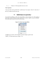
17 VERDI Batch Script Editor ................................................................................................100
17.1 Specify hour/time step formula in batch script mode ...................................................106
17.2 Mathematical function capability in batch script mode ................................................108
17.2.1 Batch Script Example: Maximum Ozone – layer 1 (Figure 17-11) ..................108
17.2.2 Batch Script Example : Minimum Ozone – layer 1 (Figure 17-12) .................109
17.2.3 Batch Script Example : Mean of Ozone – layer 1 (Figure 17-13) ....................110
17.2.4 Batch Script Example : Sum of Ozone – layer 1 (Figure 17-14) ......................111
18 Command Line Scripting ....................................................................................................112
18.1 Example Command Line Script for Linux Users .........................................................112
18.2 Example Command Line Script for Windows Users ....................................................113
19 Areal Interpolation Calculations ........................................................................................118
20 Licenses for JAVA Libraries used by VERDI ..................................................................119
Acknowledgments ......................................................................................................................120
Data Contributions .................................................................................................................120
Data Reader Contributions .....................................................................................................120
I/O Service Provider (IOSP) Interface for CAMx: .......................................................120
Incorporating the IOSP into netCDF netcdf-java v4.1 Library: ...................................120
UNC–Chapel Hill
v
Institute for the Environment
User’s Manual for VERDI 1.4.1
UNC–Chapel Hill
vi
Institute for the Environment
User’s Manual for VERDI 1.4.1
Figures
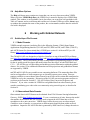
Figure 1-1. Top of Main VERDI Web Site Page .............................................................................3
Figure 1-2. Downloading VERDI from the CMAS Web Site, Step 1 .............................................4
Figure 1-3. Downloading VERDI from the CMAS Web Site, Step 2 .............................................5
Figure 1-4. Downloading VERDI from the CMAS Web Site, Step 3 .............................................6
Figure 1-5. Getting Documentation on VERDI from the CMAS Web Site ....................................7
Figure 1-6. VERDI Documentation on the CMAS Web Site ..........................................................8
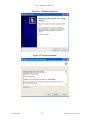
Figure 3-1. VERDI Setup Wizard..................................................................................................13
Figure 3-2. License Agreement......................................................................................................13
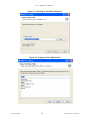
Figure 3-3. Selecting an Installation Directory ..............................................................................14
Figure 3-4. Setting the Start Menu Folder .....................................................................................14
Figure 3-5. File Extraction .............................................................................................................15
Figure 3-6. Installation Complete ..................................................................................................16
Figure 4-1. Starting VERDI in Windows ......................................................................................18
Figure 4-2. VERDI Main Window ................................................................................................20
Figure 5-1. VERDI Main Menu Options .......................................................................................21
Figure 5-2. Animate Plots Dialog and Fast Tile Plots ...................................................................23
Figure 6-1. Observational File ASCII Format ...............................................................................25
Figure 6-2. Open Dataset File Browser .........................................................................................26
Figure 6-3. Datasets Pane Displaying Information about a Dataset ..............................................27
Figure 6-4. Available Hosts in the Remote File Access Browser ..................................................28
Figure 6-5. Select one or more variables from Remote Dataset ....................................................29
Figure 6-6. Remote Dataset Labeled with Number at End of the Filename ..................................31
Figure 6-7. Edit configure.properties file to add a remote host .....................................................32
Figure 6-8. Right Click on Variable in Dataset Pane.....................................................................33
Figure 6-9. Dataset Metadata Information .....................................................................................34
Figure 7-1. Adding Multiple Variables to Formula Editor ............................................................36
Figure 8-1. Areas Pane ...................................................................................................................39
Figure 8-2. Open Area File Browser..............................................................................................40
Figure 8-3. Open Area File: Select Name Field ............................................................................40
Figure 8-4. Coordinate System ......................................................................................................41
Figure 8-5. Projection Information ................................................................................................41
UNC–Chapel Hill
vii
Institute for the Environment
User’s Manual for VERDI 1.4.1
Figure 8-6. Additional Data Fields appear depending on projection selected. ..............................41
Figure 8-7. Area Name Fields available for Shapefile ..................................................................43
Figure 9-1. Specify Time Step Range ............................................................................................44
Figure 9-2. Edit Layer Range in Formula Pane .............................................................................45
Figure 9-3. Using the Slider to View the Domain Panel ...............................................................46
Figure 9-4. Edit Domain Dialog Box .............................................................................................46
Figure 9-5. Error obtained when incompatible subset domains are created using the
Dataset pane ...........................................................................................................................48
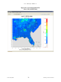
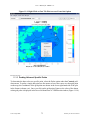
Figure 10-1. Fast Tile Plot .............................................................................................................49
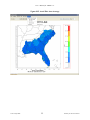
Figure 10-2. Areal Plot: Area Average ..........................................................................................52
Figure 10-3. Areal Plot: Area Totals..............................................................................................53
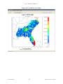
Figure 10-4. Areal Interpolation Plot: Show Grid (Gridded Data) ...............................................54
Figure 10-5. Areal Interpolation Plot: Show Selected Areas .........................................................55
Figure 10-6. Areal Values for Polygon Segments .........................................................................56
Figure 10-7. Right Click on Area Plot ...........................................................................................57
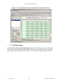
Figure 10-8. Area Information Spreadsheet ...................................................................................57
Figure 10-9. Export Spreadsheet....................................................................................................57
Figure 10-10. Name and save spreadsheet .....................................................................................57
Figure 10-11. Export Shapefile ......................................................................................................58
Figure 10-12. Name and save shapefile .........................................................................................58
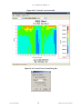
Figure 10-13. Vertical Cross Section Plot .....................................................................................59
Figure 10-14. Vertical Cross Section Dialog Box .........................................................................59
Figure 10-15. Time Series Plot ......................................................................................................60
Figure 10-16. Time Series Bar Plot ...............................................................................................61
Figure 10-17. Scatter Plot ..............................................................................................................62
Figure 10-18. Scatter Plot Dialog Box ...........................................................................................62
Figure 10-19. Scatter Plot Export Data into a CSV file .................................................................63
Figure 10-20. Vector Plot ..............................................................................................................64
Figure 10-21. Vector Plot Dialog Box ...........................................................................................64
Figure 10-22. Contour Plot ............................................................................................................65
Figure 10-23. Contour Plot Menu Options ....................................................................................65
Figure 11-1. Fast Tile and Areal Plot Pull-down Menu Options ...................................................66
Figure 11-2. Vector Plot Pull-down Menu Options .......................................................................66
Figure 11-3. Configure Plot, Titles Tab .........................................................................................69
Figure 11-4. Configure Plot, Color Map Tab ................................................................................69
Figure 11-5. Configure Plot, Labels Tab .......................................................................................69
UNC–Chapel Hill
viii
Institute for the Environment
User’s Manual for VERDI 1.4.1
Figure 11-6. Configure Plot, Other Tab .........................................................................................69
Figure 11-7. Example Plot with Tick Marks reduced for the Legend and Range Axis .................70
Figure 11-8. Right Click on Tile Plot to Zoom Out .......................................................................72
Figure 11-9. Right Click on Fast Tile Plot to access Zoom Out Option ........................................73
Figure 11-10. Click on Plot to Probe: Data Value Shown in Lower Left of VERDI, Grid
Values Shown in Lower Right ...............................................................................................74
Figure 11-11. Spreadsheet Showing Probed Values for Region of Interest ..................................75
Figure 11-12. Select Set Row and Column Ranges .......................................................................76
Figure 11-13. Enter Row and Column Values ...............................................................................77
Figure 11-14. Lat/Lon Values Shown in Lower Right of VERDI.................................................78
Figure 11-15. Plot Menu Options ..................................................................................................79
Figure 11-16. Animate Plot Dialog Box ........................................................................................80
Figure 11-17. Fast Tile Plot Observation Dialog ...........................................................................81
Figure 11-18. Fast Tile Plot with Multiple Observational Data Overlays with Grid Lines...........82
Figure 11-19. Vector Overlay Dialog Box ....................................................................................83
Figure 11-20. Wind Vector Overlay on an Ozone Fast Tile Plot ..................................................84
Figure 11-21. Plot Menu Options ..................................................................................................84
Figure 11-22. Add Map Layers ......................................................................................................85
Figure 11-23. shape2bin command usage ......................................................................................86
Figure 11-24. Manage Layers Dialog Box ....................................................................................87
Figure 11-25. Add Layer Pop-up Window ....................................................................................88
Figure 11-26. Edit Layer Pop-up Window ....................................................................................89
Figure 12-1. Lambert Conformal Conic Map Projection Example Plot ........................................90
Figure 12-2. Polar Stereographic Map Projection Example Plot ...................................................91
Figure 12-3. Mercator Map Projection Example Plot ....................................................................92
Figure 12-4. UTM Map Projection Example Plot .........................................................................93
Figure 12-5. Example CAMx diagnostic text file..........................................................................94
Figure 12-6. Models-3 I/O API Map Projection Parameters for Lambert .....................................94
Figure 12-7. Sample Projection File: camxproj.txt........................................................................95
Figure 12-8. CAMx Example Plot .................................................................................................95
Figure 17-1. File: View Script Editor ..........................................................................................100
Figure 17-2. Open Pop-up Window .............................................................................................101
Figure 17-3. Top of Sample Script File – VERDI_1.4.1/data/scripts/file_patterns.txt ...............102
Figure 17-4. Bottom of Sample Script File – VERDI_1.4.1/data/scripts/tile_patterns.txt ..........102
Figure 17-5. Close Dataset(s) Warning Message ........................................................................103
Figure 17-6. Highlight Text to Select Task and Click Run .........................................................104
UNC–Chapel Hill
ix
Institute for the Environment
User’s Manual for VERDI 1.4.1
Figure 17-7 Successful Batch Script Run Message .....................................................................105
Figure 17-8. Unsuccessful Batch Script Run Message: File not found .......................................105
Figure 17-9. Plot Image Generated by Task Block......................................................................106
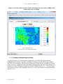
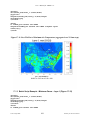
Figure 17-10. Fast Tile Plot of Ozone at Time step 17, Layer 1 .................................................108
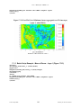
Figure 17-11. Fast Tile Plot of Maximum Air Temperature (aggregated over 25 time steps) ....109
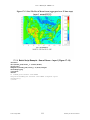
Figure 17-12. Fast Tile Plot of Minimum Ozone (aggregated over 25 time steps) .....................110
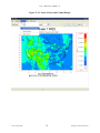
Figure 17-13. Fast Tile Plot of Mean Ozone (aggregated over 25 time steps) ............................111
Figure 17-14. Fast Tile Plot of the Sum of Ozone (aggregated over 25 time steps) ...................112
Figure 18-1. Location of run.bat script in Windows ....................................................................114
Figure 18-2. Submit run.bat script from Run command ..............................................................115
UNC–Chapel Hill
x
Institute for the Environment
User’s Manual for VERDI 1.4.1
1
Introduction
1.1 Background
This manual describes how to use the Visualization Environment for Rich Data Interpretation
(VERDI). VERDI is a flexible and modular Java-based visualization software tool that allows
users to visualize multivariate gridded environmental datasets created by environmental
modeling systems such as the Community Multiscale Air Quality (CMAQ) modeling system and
the Weather Research and Forecasting (WRF) modeling system. These systems produce files of
gridded concentration and deposition fields that users need to visualize and compare with
observational data both spatially and temporally. VERDI can facilitate these types of analyses.
Initial development of VERDI was done by the Argonne National Laboratory for the U.S.
Environmental Protection Agency (EPA) and its user community. Argonne National
Laboratory's work was supported by the EPA though U.S. Department of Energy contract DEAC02-06CH11357. Further development has been performed by the University of North
Carolina Institute for the Environment under U.S. EPA Contract No. EP-W-05-045 and EP-W09-023, by Lockheed Corporation under U.S. EPA contract No. 68-W-04-005, and Argonne
National Laboratory. VERDI is licensed under the Gnu Public License (GPL) version 3, and the
source code is available through verdi.sourceforge.net. Instructions for developers within the
community are included in the Developer User Guide (see Section 1.3). VERDI is supported by
the Community Modeling and Analysis System (CMAS) Center under U.S. EPA Contract No.
EP-W-09-023. The batch script and VERDI Script Editor were developed and documented under
U.S. EPA Contract No. EP-D-07-102, through an Office of Air Quality Planning and Standards
project managed by Kirk Baker. The CMAS Center is located within the Institute for the
Environment at the University of North Carolina at Chapel Hill.
This guide describes VERDI version 1.4.1 released in April 2013.
The following are useful web links for obtaining VERDI downloads and support:
1. VERDI Visualization Tool web site:
http://www.verdi-tool.org
2. CMAS download page for users of VERDI:
http://www.cmascenter.org/download/software.cfm
3. CMAS SourceForge.net website for developers of VERDI:
http://sourceforge.net/projects/verdi/
4. VERDI Frequently Asked Questions (FAQs):
http://www.verdi-tool.org/VERDI.faq.html
UNC–Chapel Hill
1
Institute for the Environment
User’s Manual for VERDI 1.4.1
5. To query M3USER listserv for VERDI related technical support questions and answers:
http://lists.unc.edu/read/?forum=m3user
6. To query bugs and submit bug reports, questions, and/or requests:
http://bugz.unc.edu/enter_bug.cgi?product=VERDI
(If you do not already have a login and password, click the “Home” link for instructions
on how to obtain them.)
1.2
Where to Obtain VERDI
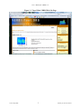
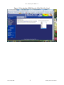
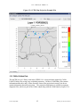
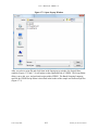
You can download the latest version of VERDI from http://www.verdi-tool.org/ (see Figure 1-1).
When you click on the link to download VERDI, you will be sent to the CMAS Model
Download Center. To download and install VERDI, follow the instructions below, skipping
step 2. Alternatively, you may also begin at the CMAS web site http://www.cmascenter.org, and
follow the instructions below:
1. Log in using an existing CMAS account, or create a new CMAS account.
2. Hover the cursor over the Download Center link on the left-hand side of the web site and
choose MODELS from the menu that appears.
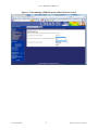
3. Select a model family to download, as shown in Figure 1-2. Use the pull-down list to
select VERDI, and then click Submit.
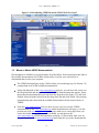
4. Select the product you wish to download, as shown in Figure 1-3. Also specify the type
of computer you are planning to run VERDI on (such as Linux PC, Windows, or Other)
from the items in the scroll list. Note that the compilers question is not relevant for
VERDI so it can be skipped. Finally, click Submit.
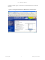
5. In the table that appears, follow the links to the Linux or Windows installation
instructions, the release notes file, the user’s manual, the test documentation, and either a
zip archive for Windows or a gzipped tar archive for Linux (see Figure 1-4).
UNC–Chapel Hill
2
Institute for the Environment
User’s Manual for VERDI 1.4.1
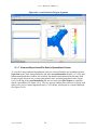
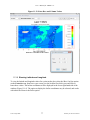
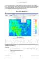
Figure 1-1. Top of Main VERDI Web Site Page
UNC–Chapel Hill
3
Institute for the Environment
User’s Manual for VERDI 1.4.1
Figure 1-2. Downloading VERDI from the CMAS Web Site, Step 1
UNC–Chapel Hill
4
Institute for the Environment
User’s Manual for VERDI 1.4.1
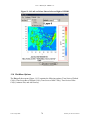
Figure 1-3. Downloading VERDI from the CMAS Web Site, Step 2
UNC–Chapel Hill
5
Institute for the Environment
User’s Manual for VERDI 1.4.1
Figure 1-4. Downloading VERDI from the CMAS Web Site, Step 3
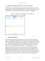
1.3 Where to Obtain VERDI Documentation
Documentation is available in several locations, described below. Each location provides links to
the available documentation for VERDI, which can be viewed in your web browser or
downloaded and saved to your computer.
The VERDI download page on the CMAS website (accessed using step 4 in Section 1.2)
contains links to all of the available documentation.
On the left-hand side of the www.cmascenter.org web site, you can hover the cursor over
the Help Desk link and choose DOCUMENTATION from the menu that appears. Select
the product documentation that you want from the drop-down list (Figure 1-5) and click
Submit. Select the model release from the drop-down list and click Search. The resulting
documentation pane shows that the available documentation for the chosen release of
VERDI.
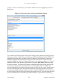
From the www.verdi-tool.org web site, there are two ways to access the VERDI
documentation on the www.cmascenter.org model documentation web page: (1) A link
near the top of the www.verdi-tool.org home page sends you to a new page where you
choose the model version. When you click submit, you are taken to the
www.cmascenter.org VERDI documentation web page. (2) Direct links from a box on
the right-hand side of the www.verdi-tool.org home page take you to the documentation
UNC–Chapel Hill
6
Institute for the Environment
User’s Manual for VERDI 1.4.1
available for VERDI. Figure 1-6 shows the list of documentation that is available for
download.
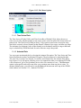
Figure 1-5. Getting Documentation on VERDI from the CMAS Web Site
UNC–Chapel Hill
7
Institute for the Environment
User’s Manual for VERDI 1.4.1
Figure 1-6. VERDI Documentation on the CMAS Web Site
1.4 Help Desk Support for VERDI
You are encouraged to check the VERDI FAQs, search archived support requests using the webbased Bugzilla system, search the M3USER listserv for VERDI-related technical support
questions, and report errors and/or requests for enhancement to the m3user forum. The m3user
forum is supported by the community and also by CMAS to help users resolve issues and
identify and fix bugs found in supported software products.
1.5 Future VERDI Development
As stated in Schwede et al. (2007),1 “VERDI is intended to be a community based visualization
tool with strong user involvement.” The VERDI source code is available to the public under a
GPL license at http://sourceforge.net/projects/verdi/. This allows users who wish to make
improvements to VERDI to download the software, and to develop enhancements and
improvements that they feel may be useful to the modeling community. Examples could include
user-developed readers for additional file formats and modules for additional plot types. Users
may wish to contribute data analysis routines, such as adding the ability to do bilinear
1
Schwede, D., N. Collier, J. Dolph, M.A. Bitz Widing, T. Howe, 2007: A New Tool for Analyzing CMAQ
Modeling Results: Visualization Environment for Rich Data Interpretation (VERDI). Proceedings, CMAS 2007
Conference.
UNC–Chapel Hill
8
Institute for the Environment
User’s Manual for VERDI 1.4.1
interpolation (smoothing), or to contribute other enhancements to the existing plot types. The
direction of future development will depend on the resources and the needs of the modeling
community. If you are interested in contributing code to VERDI, please review the information
in Chapter 14, “Contributing to VERDI Development.”
2
Requirements for Using VERDI
2.1 Java Runtime Environment
VERDI requires version 6 of the Java Standard Edition Runtime Environment (JRE). The JRETM
6 is provided as part of the VERDI release for Linux 32 bit and Windows. Instructions for how
to download JRETM 6 and the additional third-party libraries for Linux 64 bit are provided in
section 3.2. On Windows 32 bit machines, the contour plot requires DirectX SDK. Download
and install this software if you obtain the following error when running the contour plot.
http://www.microsoft.com/en-us/download/details.aspx?id=6812
2.2 Memory and CPU Requirements
VERDI’s memory and CPU requirements largely depend on the size of the datasets to be
visualized. Small datasets can be visualized and manipulated using less than 1024 megabytes of
RAM, while larger datasets may need considerably more. If you are using datasets that require
either more or less than 1024 MB of memory, you can change the default maximum memory
setting used by VERDI:
On Windows, edit the Verdi.ini file to specify a different heap size from the
default 1024M.
On Linux or another Unix platform, you can edit verdi.sh and replace the
1024 in –Xmx1024M with a different value; for example, -Xmx2048M will
allow VERDI to access up to 2048MB (or 2GB) of RAM.
Note that even slower CPUs can quickly view and animate smaller datasets, whereas larger
datasets can take longer. Initially, VERDI’s performance was slow when it was used across the
UNC–Chapel Hill
9
Institute for the Environment
User’s Manual for VERDI 1.4.1
network via ssh. This problem was addressed in version 1.1 with the addition of the Fast Tile
Plot. Beginning with version VERDI 1.4, memory was more effectively managed. As a user
opens new Fast Tile plots or other plot types, the memory requirements increase. As the user
then closes the plots, the memory is correctly released by VERDI.
2.3 Requirements to Run VERDI Remotely
VERDI may be used to run on a remote compute server and have the graphics display locally on
your desktop machine (Unix workstation, Mac, or PC) using the Fast Tile Plot. Your computer
needs to be configured to run X-Windows. Typically, you will connect to the remote compute
server using secure shell (SSH). If you are using an X-Server and wish to generate 3-D plots
using Open GL, you need to turn on Open GL support within the X-Server.
2.4 Graphics Requirements
Three-dimensional contour plots require a graphics card with OpenGL or DirectX capability. By
default VERDI uses OpenGL for 3D rendering. If you would like to use DirectX instead, add the
line: j3d=-Dj3d.rend=d3d to the verdi.ini file.
2.5 Display Properties
VERDI works best on screen displays that have been set to a high or perhaps the highest screen
resolution (1280 1024 pixels for Windows XP machines or 1440 900 for Mac or Windows
Vista). To adjust your screen resolution for a Windows XP machine, right click on your desktop
and then click on the Settings tab in the pop-up window. Use the slider under the screen
resolution section to set the resolution to 1280 1024 pixels. You may need to reboot your
computer for this modified screen setting to take effect. For Windows Vista, right click on your
desktop and click on Graphics Properties. In the pop-up window, click on Display Settings. To
adjust the screen resolution on a Mac, go to Applications and double click on System
Preferences, then under Hardware select Displays. Select 1440 900.
3
VERDI Installation Instructions
3.1 VERDI Installation
Installing VERDI on a Windows operating system is accomplished by running a standard
installer program. For Linux and other non-Windows platforms, VERDI is distributed as a
gzipped tar file that contains the executable application and the third-party libraries needed for
VERDI. Currently, the VERDI distributions provide a platform-specific Java Runtime
Environment 6.0 (see Section 3.3) for Windows and Linux. Note that the version of Java
provided with VERDI includes the JAVA 3D and JAI packages to support the three-dimensional
plots used by VERDI’s contour plot. For more information on supporting the contour plot on
your non-windows platform of interest, see the Java3D discussion section 3.2 that follows.
UNC–Chapel Hill
10
Institute for the Environment
User’s Manual for VERDI 1.4.1
Instructions on how to download JRETM 6 for other system configurations that run it are also
provided.
3.2 Installation Instructions for Linux and Other Non-Windows JRE™ 6
Supported System Configurations
Follow these instructions to install VERDI:
1. tar -xvf verdi_1.4.1.tar into a location where you would like to install VERDI.
2. Edit verdi_1.4.1/verdi.sh: Change the path for the VERDI_HOME variable to reflect the
location where VERDI was installed (e.g., VERDI_HOME=/usr/local/verdi)
3. VERDI should now run if you execute the verdi.sh executable script (e.g., ./verdi.sh).
3.3 Installation Instructions for computer that that requires a JRETM 6 other than
what was provided in the distribution:
1. Download Java 6 for your platform from http://www.java.com/en/download/manual.jsp.
2. Download Java3D
a. For all platforms, go to http://java.sun.com/javase/technologies/desktop/java3d/
b. Go to download section, click on Download Java 3D 1.5.1 Software, select your
platform, agree to license agreement, and continue.
c. mv java3d-1_5_1-linux-i586.bin to the jre1.6.0_06 directory
d. chmod a+x java3d-1_5_1-linux-i586.bin
e. ./java3d-1_5_1-linux-i586.bin (this will place the lib/ext and lib/i386 files where
they are needed)
3. Download JAI 1.1.3
a. For all platforms, go to
http://download.java.net/media/jai/builds/release/1_1_3/ Select JRE Install
(Note JRE is the Java Runtime Environment and needed for running VERDI,
JDK is the Java Development Kit, and the JDK is only needed by those who
are developing code for VERDI)
b. Download the .tar.gz package and untar. This will create a directory "jai1_1_3".
c. Copy the following files:
i. cp jai-1_1_3/lib/libmlib_jai.so /path-to-/verdi_1.4.1/jre1.6.0_13/lib/i386
UNC–Chapel Hill
11
Institute for the Environment
User’s Manual for VERDI 1.4.1
ii. cp jai-1_1_3/lib/*.jar /path-to-/verdi_1.4.1/jre1.6.0_13/lib/ext
4. Download JAI ImageIO
a. Download jai_imageio-1_1-lib-{yourplatform}.exe by clicking on it and saying
save as. Run the executable by double clicking on it to start the InstallShield
Wizard. Specify the Destination Folder as the location where the JRE was
installed.
If JRETM 6 is already installed on your Linux platform, and you would like to use the already
installed version, you will need to add Java 3D support. Copy the following files from the
version of Java provided in the VERDI release into the JRE_HOME/bin directory used by your
version of Java:
j3dcore-d3d.dll
j3dcore-ogl.dll
j3dcore-ogl-cg.dll
j3dcore-ogl-chk.dll
j3dutils.dll
3.4 Installation Instructions for Windows
To install VERDI for Windows, run the installation program VERDI_1.4.1_Installer.exe on your
Windows machine. Follow the instructions on the installation windows that appear, as shown in
Figures 3-1 through 3-6. If you are unable to install VERDI on your computer, please check to
see whether your user account is authorized to install software. You may need to request that a
user with a computer administrator account install VERDI, or provide you with an account that
has permission to install software. For more information about user account types, click Start
and select Control Panel and then click on the User Account icon.
UNC–Chapel Hill
12
Institute for the Environment
User’s Manual for VERDI 1.4.1
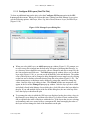
Figure 3-1. VERDI Setup Wizard
Figure 3-2. License Agreement
UNC–Chapel Hill
13
Institute for the Environment
User’s Manual for VERDI 1.4.1
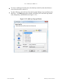
Figure 3-3. Selecting an Installation Directory
Figure 3-4. Setting the Start Menu Folder
UNC–Chapel Hill
14
Institute for the Environment
User’s Manual for VERDI 1.4.1
Figure 3-5. File Extraction
UNC–Chapel Hill
15
Institute for the Environment
User’s Manual for VERDI 1.4.1
Figure 3-6. Installation Complete
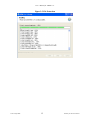
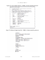
3.5 Setting VERDI Preferences
The VERDI installation package contains a file called config.properties.TEMPLATE. On
Windows, this file is copied into the VERDI subdirectory of your USERPROFILE directory
(e.g., “C:\Documents and Settings\yourusername\verdi”) and renamed to config.properties. On
Linux, this file is copied into the ~username/verdi/ subdirectory and renamed to
config.properties. Users are encouraged to edit this file to specify default directories for saving
files, for placing the location of configuration files, and for saving project files. Contents of
config.properties.TEMPLATE:
# This file should be put in $USER_HOME/verdi/ subdirectory
# Please use double backslash for windows platform or slash for UNIX like platforms as file
# Please uncomment the following lines and modify them to suit your local settings
# Windows example settings format
UNC–Chapel Hill
16
Institute for the Environment
User’s Manual for VERDI 1.4.1
# verdi.project.home=C:\\Program Files\\VERDI_1.4.1\\project
# verdi.config.home=C:\\Program Files\\VERDI_1.4.1\\config
# Linux example settings format
verdi.project.home=../../data/project
verdi.config.home=../../data/configs
verdi.user.home=../../data/model
verdi.dataset.home=../../data/model
verdi.script.home=../../data/scripts
# WDT default area file folder
verdi.hucData=../../data/hucRegion/
# For VERDI to access remote big netCDF data files
verdi.remote.hosts=terrae.nesc.epa.gov,vortex.rtpnc.epa.gov,garnet01.rtpnc.epa.gov,tulip.rtpnc.e
pa.gov
remote.file.util=/usr/local/bin/RemoteFileUtility
verdi.remote.ssh=/usr/bin/ssh
#on local machine where VERDI is running. Used to hold temporary data file downloaded from
a remote machine
verdi.temporary.dir=C:\\temp
The items in the config.properties.TEMPLATE file that is installed with VERDI are commented
out, and will need to be uncommented by removing the starting ‘#’ sign if you do not want to
specify the directories each time a file is loaded or saved. Example settings that are provided in
the default file show how to specify the paths to these locations, depending on whether the
installation is for a Windows or Linux platform. The verdi.project.home setting specifies the
default location from which to load and save projects. The verdi.config.home setting specifies
UNC–Chapel Hill
17
Institute for the Environment
User’s Manual for VERDI 1.4.1
the default location from which to load and save plot configurations. The verdi.dataset.home
setting specifies the default location from which to load datasets. The verdi.script.home setting
specifies the default location from which to load and save batch scripts. Note that VERDI stores
the most recently used directory for each of these functions and will go to that directory when
you repeat the load or save. The verdi.hucData setting specifies the default locations where area
shapefiles are located. VERDI will navigate to this directory when the user selects to add a
dataset in the Area pane. The verdi.remote.hosts setting contains a list of machines that the user
can select to browse from when adding a remote dataset using VERDI’s Remote File Access
capability. The verdi.remote.util setting specifies the location of the RemoteFileUtility script for
Linux and Mac installations of VERDI. Starting in VERDI version 1.4, the ui.properties file was
removed, and the user configurable settings such as the default directory location that were
previously specified in the ui.properties file were moved to the config.properties file.
4
Starting VERDI and Getting Your Data into VERDI
4.1 Starting VERDI
4.1.1 Windows
To start VERDI, open the Start menu, then highlight the Programs directory, followed by the
VERDI directory, and then select the VERDI icon, as shown in Figure 4-1.
Figure 4-1. Starting VERDI in Windows
4.1.2 Linux and Other Non-Windows JRETM 6 Supported System Configurations
To start VERDI from Linux and other non-Windows JRETM 6 Supported System Configurations,
find the directory where VERDI was installed, then run the verdi.sh script. On a Mac go to the
/Applications/verdi_1.4.1 directory and run the verdi.command script.
UNC–Chapel Hill
18
Institute for the Environment
User’s Manual for VERDI 1.4.1
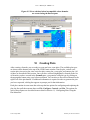
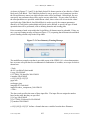
4.2 Main Window
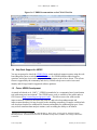
After starting VERDI, the main window will come up on the screen (Figure 4-2). At the top of
the main window, there is a menu bar with the main window options (File, Plots, Window, and
Help). Below the menu bar there are three icons that are shortcuts to some of the options
available in the Main Window Menu Bar; the first is an Open Project icon, the second is a Save
Project icon, the third is an icon that allows you to Undock All Plots. These shortcuts and the
options available in the Main Window Menu Bar are discussed further in Section 5, “Navigating
VERDI’s Main Menu Options.” Next to these three shortcut icons are buttons that list all of the
available plot types. To the right of all the plot buttons the Selected Formula is listed. The
Selected Formula refers to the formula that has been selected in the Formula pane (discussed
briefly below and in detail in Section 7), and that will be used to create plots. Below the icons
and plot buttons, the window is divided into two main areas: a parameters area on the left side
and a plots area on the right side. The parameters area contains three tabbed panes:
The Datasets pane is used to load in the dataset files that you want to work with in this
session (this is discussed in Section 6). Once the datasets are loaded, VERDI
automatically displays the lists of variables that are in the datasets. To see the variables in
a dataset, click on the dataset, and the variables will be displayed in the Variables panel
underneath the list of datasets. In Version 1.05 and later, if you double click on the name
of a variable listed on the variables panel, the variable will automatically be added as a
formula on the Formula pane and will be the default formula for new plots that are
created.
The Formula pane is used to create a formula that refers to the variable and the dataset
that you are interested in plotting (see Section 7 for more information). All plots in
VERDI are generated from formulas. A formula can be as simple as a single variable
from one dataset or it can be an equation that uses variable(s) from one or more datasets.
The Areas pane is used to load area files that are used to create areal interpolation plots
(see Section 8 for more information). Area files are defined as shapefiles that contain
area features such as watersheds and counties, or any other shapefile that consists of a set
of closed polygons.
Any plots that are created are shown in the plots area on the right-hand side of the main window.
These plots can be placed into their own movable windows using Plots>Undock all Plots on
VERDI’s main menu, as discussed in Section 5.2.1. The fast tile plot option was added in
VERDI version 1.1. As of VERDI 1.4, the tile plot option was removed, since the functionality
has been replaced by the fast tile plot; however, there are derivative plots, such as the vector plot,
that still use the tile plot code. In a future release, these derivative plots will be migrated to use
the Fast Tile Plot as their base. The Fast Tile Plot has an option (Plot>Add Overlay> Vectors) to
create a Fast Tile Plot of a variable with a vector overlay of wind vectors or other vector types.
The Fast Tile Plot with vector overlay should be used as the preferred alternative to the Vector
Plot until the Vector Plot is updated in a future release. The functions that are currently enabled
for fast tile plots are described in Section 10, “Creating Plots.”
UNC–Chapel Hill
19
Institute for the Environment
User’s Manual for VERDI 1.4.1
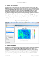
Figure 4-2. VERDI Main Window
4.3 Floating the Dataset and Formula Panes
The Formula, Dataset, and Areas panes can each be configured to float, to allow you to
position them alongside one another. To allow a pane to float, click the icon at the top of the
pane that looks like a rectangle with an angle bracket above the upper right corner. You can then
click on the pane and move it independently of the VERDI main window. This is useful when
you are entering a formula in the Formula pane, if you have difficulty remembering the
variables that are in a loaded dataset. Once a pane is unconnected from the frame, the icon
changes to be a box with an arrow pointing inward, with the hover over text tip: “Connects this
panel to the frame”. Click on the box with the inward arrow to reconnect the panel with the
frame. This will return the floating pane back to where it usually lives within the main window.
5
Navigating VERDI’s Main Menu Options
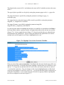
Figure 5-1 shows a graphic of the main menu options that are available on the top menu bar in
VERDI’s main window (Figure 4-2 above). These options are discussed in detail below.
UNC–Chapel Hill
20
Institute for the Environment
User’s Manual for VERDI 1.4.1
Figure 5-1. VERDI Main Menu Options
VERDI
About
VERDI
Preferences
Services
File
Open Project
Save Project
Save Project As
View Script Editor
Exit
Plots
Undock All Plots
Animate Tile
Plots
Window
Areas
Datasets
Formulas
Help
VERDI Help
Docs
About
Quit VERDI
5.1 File Menu Options
5.1.1 Open Project
Open Project retrieves projects that were saved during a previous session (using the two Save
Project options described next). Note that when you use a saved project, it is very important to
load that project into VERDI before you load any additional datasets or create any additional
variables/formulas. If you load a dataset that is not part of the previously saved project and then
try to open a previously saved project, you will get a message that says “All currently loaded
datasets will be unloaded”, and will be asked if you want to continue.
5.1.2 Save Project
The Save Project and Save Project As options save dataset lists and associated formulas as a
“project” for later re-use.
Note that plots are not saved with a project; only datasets and formulas are saved. If you wish to
save a plot configuration for later use, see Section 11.2.2, “Loading and Saving configuration.”
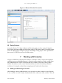
5.1.3 View Script Editor
The View Script Editor allows users to modify and run batch scripts within VERDI. Three
sample script files are provided with the VERDI distribution under the
$VERDI_HOME/data/scripts directory. On a Windows machine the $VERDI_HOME is
typically C://Program Files//VERDI_1.4.1. Use the Open pop-up window to specify eps.txt, one
of the sample script files. The contents of the eps.txt will be displayed in the Script Editor in the
right side of the VERDI window. Modify it to specify the local directory path name for the
sample data files, the formulas, the type of plots, and the image format. The plots are not
rendered within VERDI, but may be viewed using an image viewer. The batch scripting
language is described in the sample script files, and will be described in more detail in Section
17: VERDI Script Editor.
UNC–Chapel Hill
21
Institute for the Environment
User’s Manual for VERDI 1.4.1
5.2 Plots Menu Options
VERDI opens a single window for plots, to the right of the Dataset, Formula, and Area panes.
As plots are created (each in its own sub-window), the most recent plot is displayed on top of
previously created plots. Each plot has a tab beneath it listing the type of plot and the formula
used to create it. If you want to view a previously created plot, select the tab associated with its
sub-window underneath the current plot, and the desired plot will be brought to the front.
5.2.1 Undock All Plots
As with the Dataset, Formula, and Area panes (Section 4.3), plot sub-windows can be
undocked or externalized so that you can move them into separate, floating windows. This
allows side by side comparisons of plots. Note that undocking is performed only on previously
created plots; any newly created plots are created within the VERDI main window.
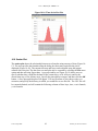
5.2.2 Animate Tile Plots
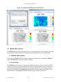
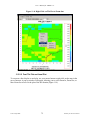
This option opens an Animate Plots dialog box (Figure 5-2) that allows you to select one or
more plots, select a subset of the time range, and create an animated GIF file. There is also a
separate way to create a Quicktime movie instead of a GIF, if desired.
Within the Animate Plots dialog box, you can select plot(s) to animate by clicking the check
box beside each plot name.
You can choose to animate a single plot, or animate multiple plots synchronously. To view
multiple animated plots synchronously, undock the plots (see Section 5.2.1) and move them so
that they are located side by side for visual comparison during the animation.
Once a plot has been selected, you can select the time range by specifying both the starting
time step and ending time step of the animation.
To create an animated GIF, check the Make Animated GIF(s) option in the Animate Plots
dialog box. In the Save dialog box that appears, select the directory in which to store the file and
the name to use for the animated GIF, then click the save button. When saving as an animated
GIF, when multiple plots are selected, each animated plot will be saved to a separate animated
GIF file. For example, if three plots were selected, the animated plots would be saved as
<filename>-1.gif, <filename>-2.gif, <filename>-3.gif. You can view the animated GIF by
opening the file in a web browser.
Creating a Quicktime movie is also an option, but this is not done through the Plots>Animate
Tile Plots main menu option. Instead, use the Plot menu option found at the top of each
individual plot to make a Quicktime movie.
UNC–Chapel Hill
22
Institute for the Environment
User’s Manual for VERDI 1.4.1
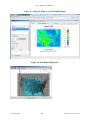
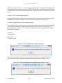
Figure 5-2. Animate Plots Dialog and Fast Tile Plots
5.3 Window Menu Options
The Window menu provides an alternate way to select windows/panes to be brought to the front,
and provides the same function as clicking on the tabs at the bottom of the windows/panes.
5.3.1 Datasets and Formulas
Select from the Window pull-down menu to bring to the front either the Areas pane, Datasets
pane or Formulas pane when those panes are docked.
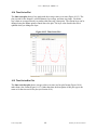
5.3.2 List of Plots
The Window pull-down menu is automatically updated each time a plot is created in a VERDI
session; each entry in the plot list indicates the type of plot and the formula used. Clicking on a
given plot entry brings that plot to the front for viewing. Alternatively, you can bring a plot to
the front by selecting the desired plot tab underneath the plots area of the main window. As in
the menu entries, each plot tab is labeled with the plot type and the formula used.
UNC–Chapel Hill
23
Institute for the Environment
User’s Manual for VERDI 1.4.1
5.4 Help Menu Options
The Help pull-down menu contains two items that you can use to learn more about VERDI.
When you select VERDI Help Docs, the VERDI user’s manual is displayed in a VERDI Help
window. This window is not searchable, but it does allow you to navigate via hyperlinks in the
Table of Contents, and to scroll down and read the user’s manual. When you select About a popup window that contains the name of the product, the version number, and the date the software
was built is displayed.
6
Working with Gridded Datasets
6.1 Gridded Input File Formats
6.1.1 Model Formats
VERDI currently supports visualizing files in the following formats: CMAQ Input/Output
Applications Programming Interface (I/O API) netCDF, WRF netCDF, and CAMx (UAM-IV),
and ASCII format (for observational data). VERDI uses version 4.1 of the netCDF java I/O
library (http://www.unidata.ucar.edu/software/netcdf-java).
The CMAQ I/O API was designed as a high-level interface on top of the netCDF Java library.
(see http://www.baronams.com/products/ioapi and http://www.unidata.ucar.edu/software/netcdf/
for further info). The I/O API library provides a comprehensive programming interface to files
for the air quality model developer and model-related tool developer, in both FORTRAN and
C/C++. I/O API files are self-describing and include projection information within the gridded
dataset. See section 12 for additional information on what projections and gridded data formats
are supported by VERDI.
netCDF and I/O API files are portable across computing platforms. This means that these files
can be read regardless of what computer type or operating system you are using. There are
routines available to convert data to these formats or new code can be written and contributed to
VERDI for use by the community. Discussion of the I/O API conversion programs and how to
use them can be found in Section 13, “I/O API Utilities, Data Conversion Programs, and
Libraries.” If you write a routine for VERDI to read gridded data from other formats, please
consider contributing your code to the user community using sourceforge.net, as described in
Section 14.
6.1.2 Observational Data Formats
Observational data in ASCII format can be obtained from EPA’s Remote Sensing Information
Gateway - RSIG (http://badger.epa.gov/rsig). To use a consistent set of units, between the model
data and the observational data, the user may need to import the ASCII data into an Excel
spreadsheet to do a unit conversion. VERDI doesn’t allow the user to use an observational
variable to create a formula, so conversions to different units should be done within an Excel
spreadsheet. Import the file ASCII file that is generated by RSIG into Excel, change the units to
UNC–Chapel Hill
24
Institute for the Environment
User’s Manual for VERDI 1.4.1
match the units found in the gridded model data file and then save using a tab delimited ASCII
file format.
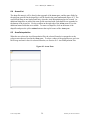
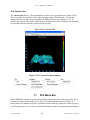
The observational data ASCII format recognized by VERDI is an ASCII file with tab-separated
columns where the first four columns are provided in the order shown in Figure 6-1 and one or
more additional columns are arbitrary but must have the header format 'name(units)' as shown in
Figure 6-1. Spreadsheet programs can be used to edit and write the files by choosing ASCII
output and tab as the delimiting character (instead of comma). Data within a column must be
complete, as empty fields within a column will cause VERDI to be unable to read the
observational data. VERDI 1.4.1 allows the user to specify an alphanumeric value (either
numbers and/or letters) for the fourth column (Station ID).
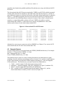
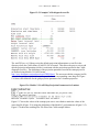
Figure 6-1. Observational File ASCII Format
Timestamp(UTC)
LONGITUDE(deg)
LATITUDE(deg)
2005-08-26T00:00:00-0000
-121.7842
37.6875
2005-08-26T00:00:00-0000
-122.3991
37.7660
2005-08-26T00:00:00-0000
-122.2034
37.4829
2005-08-26T00:00:00-0000
-121.8950
37.3485
2005-08-26T01:00:00-0000
-121.7842
37.6875
2005-08-26T01:00:00-0000
-122.3991
37.7660
2005-08-26T01:00:00-0000
-122.2034
37.4829
2005-08-26T01:00:00-0000
-121.8950
37.3485
2005-08-26T02:00:00-0000
-121.7842
37.6875
STATION(-)
060010007
060750005
060811001
060850005
060010007
060750005
060811001
060850005
060010007
pm25(ug/m3)
11.0000
12.0000
21.0000
16.0000
21.0000
22.0000
19.0000
20.0000
28.0000
Alternatively, users may use a converter such as AIRS2M3 (see Chapter 13) to convert ASCII
observational data into I/O API "observational-data" files.
6.2 Example Datasets
Several example datasets are provided under the $VERDI_HOME/data directory. For example:
Windows: C:\\Program Files\\VERDI 1.4.1\\data
Mac: /Applications/verdi_1.4.1/data/
Linux: $VERDI_HOME/verdi_1.4.1/data
These datasets may be used to re-create example plots that are provided in this user guide,
including a tile plot with observational data overlay in Section 11.4.3, and the example datasets
for the various dataset projections that VERDI supports including LCC, polar stereographic,
UTM and Mercator. The data directory currently contains four subdirectories:
1. CAMx – contains sample CAMx dataset and camxproj.txt file
2. hucRegion – contains Hydrologic Unit (HUC) shapefiles for region 3 (southeast US)
3. Model – contains sample WRF and CMAQ I/O API datasets
4. Obs – contains an ASCII formatted observational dataset (Chapter 6-1), and an
observational dataset created by airs2m3 converter (Chapter 13).
UNC–Chapel Hill
25
Institute for the Environment
User’s Manual for VERDI 1.4.1
6.3 Adding and Removing a Dataset from a Local File System
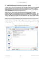
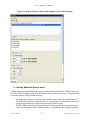
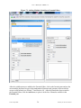
To load a data set from a local file system, press the yellow plus button at the top of the Datasets
pane. A file browser (Figure 6-2) allows you to select a dataset for use in VERDI. Support for
loading data from a remote file system has been added beginning in version 1.4. The use of the
yellow plus remote button will be discussed in Section 6.4.
After you select a dataset, VERDI will load header information and display the available
variables, time steps, layers, and domain used by the file in the Datasets pane (Figure 6-3). (The
actual model data are not loaded until later, when plots are created.) To view the variables for a
particular dataset that has been loaded, click on the dataset name in the list to highlight it, and the
variables will be listed in the panel below.
Datasets can be removed by highlighting the name of the dataset in the dataset list and pressing
the yellow minus button. Note that although the dataset will be removed, the number that was
assigned to that dataset will not be reused by VERDI during the current session (unless there had
been only one dataset loaded, and it was removed; in that case the next dataset that is loaded will
be labeled number 1).
Figure 6-2. Open Dataset File Browser
UNC–Chapel Hill
26
Institute for the Environment
User’s Manual for VERDI 1.4.1
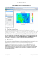
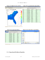
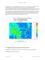
Figure 6-3. Datasets Pane Displaying Information about a Dataset
UNC–Chapel Hill
27
Institute for the Environment
User’s Manual for VERDI 1.4.1
6.4 Adding and Removing a Dataset from a Remote File System
VERDI provides users with the ability to select and add variables from datasets on remote file
systems. To do this, press the yellow plus remote (plus with a diagonal arrow) button at the top
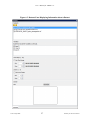
of the Datasets pane. In the Remote File Access Browser (Figure 6-4) that appears, enter your
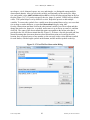
user name, choose a host from the list, and enter your password, then click Connect.
Figure 6-4. Available Hosts in the Remote File Access Browser
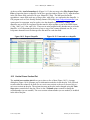
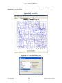
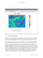
6.4.1 Remote File Browser
The top panel displays a listing of the home directory on the remote file system, as shown in
Figure 6-5. The current path is displayed in the text box and users can edit this information to
change to another directory. An alternate way to navigate between directories is using the middle
panel. In the middle panel, double click on a directory name to go into that directory, or click on
the “../” at the top of the middle panel to navigate up a directory. As you enter a directory, the
contents of the directory will be displayed as a list in the middle panel. Directory names are
followed by a “/” symbol, while filenames do not have a “/” symbol after them. View the
variables within each file of interest by double clicking on the netCDF filename listed in the
middle panel. Note: if the selected file has a format that is not supported by VERDI then the
following message will be displayed in the bottom panel: “Not a valid NetCDF file”. For
supported netCDF files, VERDI will provide a list of variables that are available within the file
in the bottom panel labeled “Select one or more variables”. To select variables from the list, use
your mouse to click on a single variable, or use either the Shift key with the mouse to select a
contiguous list of variables, or the Control key with the mouse to select a set of individual
UNC–Chapel Hill
28
Institute for the Environment
User’s Manual for VERDI 1.4.1
variables. Once the variables that you would like VERDI to read are highlighted, click on the
Read button.
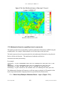
Figure 6-5. Select one or more variables from Remote Dataset
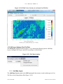
The variables read from the remote dataset will be displayed in the dataset and variable browser
in the same way that variables from a local dataset are added and displayed within VERDI. The
subsetted local dataset names are identical to the file names on the remote host, except for an
additional extension that enumerates how many times the remote files were read and saved
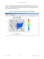
locally by VERDI (i.e., filename1, filename2, filename3, etc.), as shown in Figure 6-6. To add
additional variables from the same remote dataset, click on the plus remote button, and repeat
the above procedure. The Remote File Browser retains the login session and the directory that
was last accessed by the user, to facilitate ease of accessing remote datasets. VERDI will
increment the numerical extension to the dataset name, to allow the user to know that this subset
file was created using the same remote dataset, but that the subset file with the new numerical
extension may contain a different subset of variables. Note that VERDI does not check to see if
the same variable from the same remote dataset has already been read. Also note that subset files
read in by VERDI will be saved either to your home directory on your local file system (e.g.,
UNC–Chapel Hill
29
Institute for the Environment
User’s Manual for VERDI 1.4.1
C:\Documents and Settings\username on a Windows XP machine), or to the location that is
specified in the config.properties file using the verdi.temporary.dir setting. Refer to Section 6.4.2
on how to edit and save the config.properties file. The files are saved on your local machine to
facilitate project management. To be able to save and then load a project for future use, the files
need to be saved on the local machine. To avoid filling up your local file system, regularly
inspect the file list in the home or verdi.temporary.dir directory and manually delete unneeded
subset files.
Remote datasets can be removed from the dataset list in VERDI using the same procedure as for
removing local datasets: highlight the name of the dataset in the dataset list and press the yellow
minus button. Note that although the dataset will be removed from the dataset list, the number
that was assigned to that dataset will not be reused by VERDI during the current session.
UNC–Chapel Hill
30
Institute for the Environment
User’s Manual for VERDI 1.4.1
Figure 6-6. Remote Dataset Labeled with Number at End of the Filename
6.4.2 Adding Additional Remote Hosts
VERDI contains the RemoteFileUtility and ncvariable programs that enable VERDI to add your
I/O API netCDF or WRF netCDF formatted dataset from a remote file system. A gzipped tar file
is available in the $VERDI_HOME directory.
1. The RemoteFileUtility c-shell script and ncvariable binary need to be installed either in
/usr/local/bin by the System Administrator, or you can place it in a different location, and
specify that location in the configure.properties file located in your
$USER_HOME/verdi/ directory (see section 3.4 for the specific directory location that is
used for each platform [Linux, Windows, Mac]). A template for the configure.properties
UNC–Chapel Hill
31
Institute for the Environment
User’s Manual for VERDI 1.4.1
file called configure.properties.TEMPLATE is provided in the distribution under the
$VERDI_HOME directory (see section 3.4 for information on how to edit the settings).
2. A README file provided with the software contains instructions on how to compile the
source code if the binaries provided do not match your operating system.
3. Copy the file configure.properties.TEMPLATE to configure.properties. Edit the
configure.properties file in the $USER_HOME/verdi directory. Add the name or IP
address of the Linux server, preceded by a comma, at the end of the list of machines
defined as remote hosts in the configure.properties file, as shown in Figure 6-7. You will
need to restart VERDI in order for it to recognize a newly added remote host name.
Figure 6-7. Edit configure.properties file to add a remote host
6.5 Variables List
The variables list shows all of the variables contained in a loaded dataset (see the example in
Figure 6-7). To display a variables list, select the name of the dataset of interest in the Datasets
pane. Each of the variables in the list can be used to create a formula in the Formula pane that
can then be used to create plots. VERDI allows the user to automatically add a formula by
double clicking on the name of a variable. Double clicking on a variable will automatically
create a formula that contains the variable for the loaded dataset and it will become the default
formula for making plots. In addition, you may right click on the name of the variable to show a
popup menu as shown in Figure 6-8. From this menu you can either add the variable as a
formula, or you can to add it into the formula editor so that it can be used to compose more
complex formulas. Formulas are described in more detail in Section 7.
UNC–Chapel Hill
32
Institute for the Environment
User’s Manual for VERDI 1.4.1
Figure 6-8. Right Click on Variable in Dataset Pane
6.6 Time Steps, Layers Panels
The range that is available for the dataset is listed in the Time Steps or Layers Panel in
parenthesis next to the label for the panel, e.g. for a dataset that has 5 time steps, the range would
be displayed as: Time Steps (1-5). The user can select to use a subset of the full time step range
by clicking on the Use Time Range checkbox, and then using the Min and Max spinner controls
to set a new minimum or maximum values, for example choosing time step 2 as the minimum
time step, and time step 4 as the maximum. When a tile plot is created, it will only display time
steps 2-4. Detailed instructions for using the Time Steps, Layers, and Domain panels that you
see in Figure 6-7 are discussed in Section 9, “Spatial and Temporal Data Subsetting.”
6.7 Domain Panel
The domain panel contains an Edit button and a Metadata button. Detailed instructions for using
the Edit button are provided in Section 9, “Spatial and Temporal Data Subsetting”.
To display the metadata information about a dataset, click on the Metadata button in the
Domain panel. A window containing the metadata will appear (Figure 6-9). Each dataset
includes metadata information that is part of the file header. The metadata provided include the
map projection information, the number of time steps in the file, the number of columns and
rows, and other information.
UNC–Chapel Hill
33
Institute for the Environment
User’s Manual for VERDI 1.4.1
Figure 6-9. Dataset Metadata Information
6.8 Saving Projects
As noted in Section 5.1.2, lists of datasets and formulas can be saved as “projects” using the
Save Project option in the File pull-down menu on the VERDI main window. Refer back to that
section for discussion on saving new projects and loading existing projects. Note again that the
plots created in VERDI are not saved with the project.
7
Working with Formulas
All plots in VERDI are generated from formulas. A formula is used to compare or manipulate
variables in one or more gridded datasets. A formula can be as simple as a single variable from
one gridded dataset or it can be an equation that uses variable(s) from one or more gridded
datasets. Formulas are used to create visualizations that can assist with model performance
evaluations, for example, or that help in comparing model results with observations.
7.1 Adding and Removing a Formula
After loading the desired gridded datasets, you can use the variables in them to create formulas.
To use a variable to create a simple formula, double click on the name of the variable. This will
UNC–Chapel Hill
34
Institute for the Environment
User’s Manual for VERDI 1.4.1
add the formula <Variable Name>[<Dataset Number>] to the formula list in the Formulas
pane—for example, O3[1]. To add a variable to the formula editor window, highlight the
variable, right click on the variable name in the Datasets pane, and select Add Variable(s) to
Formula Editor. To add all or a subset of variables from the Dataset pane to the formula editor
window, click on the first variable to highlight it, hold the Shift key down and click at the last
variable that you want to include, then right click and select Add Variables(s). The formulas
that are highlighted using this method will be added to the formula editor (Figure 7-1).
UNC–Chapel Hill
35
Institute for the Environment
User’s Manual for VERDI 1.4.1
Figure 7-1. Adding Multiple Variables to Formula Editor
After the variable names are added to the Formula Editor, click on the formula pane and use the
cursor and the keyboard to type in the mathematical functions and operators where needed to
create a valid formula (see Section 7.2 and Section 16). After the formula has been created in
the Formula Editor, click the Add button, to place it in the list of formulas available in the
Formula pane.
UNC–Chapel Hill
36
Institute for the Environment
User’s Manual for VERDI 1.4.1
To remove a formula from the formulas list, highlight the name in the list and press the yellow
minus button. Note that removing a formula from the formula list does not remove plots that
were created prior to the deletion of the formula.
7.2 Example Formulas
To examine the values of ozone in dataset 1, the formula would be “O3[1]”.
To examine the difference in ozone between datasets 1 and 2, the formula would be “O3[1]O3[2]”.
To calculate the percent difference in ozone between datasets 1 and 2, the formula would be
“(O3[1]-O3[2])*100/(O3[2])”.To identify all cells where the ozone concentration exceeds a
certain value, you can use the Boolean operators to “screen out” ranges of your data that are of
particular interest. A Boolean expression will evaluate to either True = 1 or False = 0. For
example, to plot the cells in which the ozone values in dataset 1 exceed 0.080 ppm, you could
use the formula “(O3[1]>0.080)*O3[1]”. In the resulting plot, each cell where O3[1] exceeds
0.080 will show the value of O3[1] for that cell; for all other cells the value shown will be zero.
The notations that can be used in formulas to represent various mathematical functions, and the
order of precedence of these functions, are listed in Section 16, “Mathematical Functions.”
7.3 Selecting a Formula for Plotting
Before creating a plot, a formula must be selected. Check to see which formula is highlighted in
the Formula pane, or look to the right of the plot buttons above the plots area of the main
window to see the selected formula. By default, VERDI designates the most recently added
formula as the selected formula. To change the selected formula to a different one in the list,
click on a formula in the list on the Formula pane, and you will then see it displayed as the
selected formula above the plots area.
7.4 Saving Formulas
Both formulas and datasets can be saved using the Save Project item in the File pull-down menu
on the VERDI main window. Saving new projects and loading existing projects was discussed in
Section 5.1.
7.5 Time Step Range, Layer Range, and Edit Domain
Instructions for using the Time Steps, Layers, and Domain panels that you see in Figure 7-1 are
discussed in the next section, “Spatial and Temporal Data Subsetting.”
UNC–Chapel Hill
37
Institute for the Environment
User’s Manual for VERDI 1.4.1
8
Working with Area Files
8.1 Area File Formats
Area files are defined as shapefiles that contain area features such as watersheds and counties, or
any other shapefile that consists of a set of closed polygons.
The shapefile format (ESRI, 1998) consists of four files.
1.
2.
3.
4.
The *.shp file contains the actual shape vertices.
The *.shx file contains the index data pointing to the structures in the .shp file.
The *.dbf file contains the attributes (e.g., gridded concentrations).
The *.prj file contains the map projection information used for the gridded
concentrations.
8.2 Example Area File
Shapefiles that contain closed polygons are used by VERDI to interpolate gridded data to
geographic boundary regions to create Areal Interpolation Plots. Shapefiles containing state,
county, or census block, for example, or any other shapefile containing polygon areas may be
used in VERDI to calculate and map formulas to the user-selected geographic regions. An
example shapefile containing the 8-digit HUC watershed boundary map for the Southeast
(Region 3) is provided in the VERDI release under the $VERDI_HOME/data/HucRegion
directory.
Example on-line data archives for these shapefiles include:
http://datagateway.nrcs.usda.gov
http://www2.census.gov/cgi-bin/shapefiles/national-files
8.3 Adding and Removing an Area File
To load a shapefile, press the yellow plus button at the top left corner of the Areas pane (Figure
8-1). A file browser (Figure 8-2) allows you to change directories and select a shapefile file for
use in VERDI. Click on the shapefile name and click Next. The Open Area pop-up window
will be displayed next which allows you to select the name of the field to read from the file and
supply projection information if needed. Use the pull-down menu and click on the Name Field
(Figure 8-3) to be used. If a *.prj file is not provided with the dataset, the user is required to
specify the projection information. A pull-down menu will prompt the user to select the
coordinate system used in the file: either the Geographic (lat/lon) coordinate system or a
Projected (x/y) coordinate system (Figure 8-4). If the user selects Projected, an additional pulldown menu asks what type of projection, and a text box allows users to provide the required
information to do the projection (Figures 8-5 and 8-6). After the Name Field and the Coordinate
System have been specified, select Finish. The resulting plot will be in the same projection as
the gridded information used in the plot.
UNC–Chapel Hill
38
Institute for the Environment
User’s Manual for VERDI 1.4.1
8.4 Areas List
The shapefile name(s) will be listed in the top panel of the Areas pane, and the name fields for
the polygons provided in the shapefile(s) will be listed in the panel underneath (Figure 8-7). The
actual model data are not loaded until later, when the Areal Interpolation plots are created. As
additional shapefiles are added, the name fields associated with each shapefile are appended to
the bottom of the Areas list. Use the scrollbar on the right side of the Areas pane to view the
additional name fields that are available. To remove a shapefile, click on the name of the
shapefile and press the yellow minus button at the top left corner of the Areas pane.
8.5 Areal Interpolation
When the user selects the Areal Interpolation Plot, the selected formula is remapped over the
polygon areas that are listed in the Areas pane. To select a subset of the polygon areas, and view
the average and total values for selected formulas, see Section 10.3: Areal Interpolation Plot.
Figure 8-1. Areas Pane
UNC–Chapel Hill
39
Institute for the Environment
User’s Manual for VERDI 1.4.1
Figure 8-2. Open Area File Browser
Figure 8-3. Open Area File: Select Name Field
UNC–Chapel Hill
40
Institute for the Environment
User’s Manual for VERDI 1.4.1
Figure 8-4. Coordinate System
Figure 8-5. Projection Information
Figure 8-6. Additional Data Fields appear depending on projection selected.
UNC–Chapel Hill
41
Institute for the Environment
User’s Manual for VERDI 1.4.1
UNC–Chapel Hill
42
Institute for the Environment
User’s Manual for VERDI 1.4.1
Figure 8-7. Area Name Fields available for Shapefile
9
Spatial and Temporal Data Subsetting
Both the Dataset pane and the Formula pane include the three panels discussed in Sections 9.1
through 9.3: Time Steps, Layers, and Domain. Section 9.4 then discusses the precedence rules
for subsetting data that determine which pane’s subsettings (Dataset or Formula) take priority.
UNC–Chapel Hill
43
Institute for the Environment
User’s Manual for VERDI 1.4.1
9.1 Specify Time Step Range
Information about the range of time-step values included in a dataset is displayed in the Time
Steps panel (Figure 9-1). The maximum time-step range that can be used for a dataset or formula
is specified in the Min and Max spinner controls. You can use these controls to select a subset of
the available time-step range for plotting. Check the Use Time Range box above the spinner
controls to tell VERDI to use the time-step range values you have specified when it creates a
plot. By default, a plot will initially display data for the minimum time step that was specified in
the Time Steps panel. The range of the time steps available in the Time Step spinner control at
the top of the plot will reflect the subset of time steps specified when the Use Time Range box is
checked. The date and time of that time step are shown below the plot. Subsetting (also called
cropping) a dataset’s or formula’s time-step range will affect any plots made; see Section 9.4 to
learn the precedence rules.
Figure 9-1. Specify Time Step Range
9.2 Specify Layer Range
Information on the range of vertical model layers included in a dataset is displayed in the Layers
panel (Figure 9-2). You can use the Min and Max spinner controls to select a subset of the
available layer data for plotting. Check the Use Layer Range box above the spinner controls to
tell VERDI to use the layers you have specified. By default, a plot will initially display data for
the minimum layer chosen in the Layers panel. The range of the layers available in the Layer
spinner control at the top of the plot will reflect the subset of layers specified when the Use
UNC–Chapel Hill
44
Institute for the Environment
User’s Manual for VERDI 1.4.1
Layer Range box is checked. Subsetting a dataset’s or formula’s layer range will affect any
plots made; see Section 9.4 to learn the precedence rules.
Figure 9-2. Edit Layer Range in Formula Pane
9.3 Specify Domain Range
Datasets contain data for cells over a particular geographic area. In the VERDI program this area
is referred to as a “domain.” By default, the entire domain contained in a dataset is used in
creating plots. The Edit Domain dialog box can be used to select a subset of this domain for
plotting. To access the Edit Domain dialog box, first use the vertical slide bar to bring the
Domain panel (located below the Layers panel) into view if it is not already visible (Figure 9-3).
To select a subset of the domain, press the Edit button. The Edit Domain dialog box will appear
(Figure 9-4). If the area of interest is large, background data such as state and county outlines
will be shown on the map. The magnifying glass buttons above the map can be used to zoom in
and out on the map. Use the pan icon to drag the map to a position where the desired area is
displayed. To select the desired cells, first press the Select Region button. You can then drag a
box around the area of interest; selected cells will appear in blue. To clear out the selected area,
use the Clear Region button. When you are satisfied with the domain subset you have chosen,
click the OK button. Subsetting a dataset’s or formula’s domain range will affect any plots
made; see Section 8.4 to learn the precedence rules.
UNC–Chapel Hill
45
Institute for the Environment
User’s Manual for VERDI 1.4.1
Figure 9-3. Using the Slider to View the Domain Panel
Figure 9-4. Edit Domain Dialog Box
UNC–Chapel Hill
46
Institute for the Environment
User’s Manual for VERDI 1.4.1
9.4 Rules of Precedence for Subsetting Data
The subsetting feature allows the user to combine variables from two or more datasets that may
have originally contained differing layer, time step or domain ranges, when a sub-portion of the
datasets contains an identical set of layers, time steps and domain range. The user may select a
subset of the data available in the dataset so that the range selected is for an identical time step,
layer and domain range so that they may be used to create a formula and be displayed in a plot.
Because both the Dataset pane and the Formula pane have the Time Steps, Layers, and
Domain panels described above, precedence rules were established that determine which pane’s
subsettings take priority. It is important to understand these rules.
A subset of data specified in the Dataset pane takes precedence over any
subset specified in the Formula pane. At the time of this release, the range
displayed in the Formula pane does not get updated when a subset range is
selected on the Datasets pane. For example, if a dataset has a full time-step
range of 0-48, and a time-step range of 2-40 is selected on the Dataset pane,
then the 0-48 time-step range that is listed for the formula in the Formula
pane is not applicable. When a plot is then created, the time-step range subset
you chose in the Dataset pane (2-40) is displayed.
If no subsetting has been done for a particular data type (time steps, layers, or domain) in the
Dataset pane, then any subsetting done for that parameter in the Formula pane will take effect.
When a subset of data is requested in the Dataset pane, this deactivates the
ability to further subset the data for this range in the Formula pane. For
example, if the data are subset in the Dataset pane to a layer range of 2-7, and
then in the Formula pane you attempt to further subset the layer range to 4-5,
the further subsetting will be ignored and the plot will be created with a layer
range of 2-7.
When the user wants to create formulas using variables from multiple
datasets, it is important to use the Formula pane to subset the domain range
(if such subsetting is needed). The user should not try to create matching
subset domain ranges for multiple datasets using the Dataset pane for each
dataset, because if all of the subsetted domains do not match exactly, an error
will occur when the user attempts to create a formula using variables from
those datasets (Figure 9-5). Using the Formula pane instead to do the domain
subsetting allows the user to select a subset of the domain to be applied for all
dataset variables used in the selected formula.
UNC–Chapel Hill
47
Institute for the Environment
User’s Manual for VERDI 1.4.1
Figure 9-5. Error obtained when incompatible subset domains
are created using the Dataset pane
10
Creating Plots
After creating a formula, you are ready to create and view some plots. The available plot types
are shown on the buttons at the top of the VERDI main window: fast tile plot, vertical cross
section plot, time series plot, time series bar plot, scatter plot, vector plot, and contour plot. All
of these are described in this section. Once you have selected (highlighted) a formula in the list
of formulas you have created in the Formula pane, you generate each plot type by clicking on
the appropriate button using your left mouse button. You can also see the selected formula to the
right of all of the plot buttons. If additional information is required in order to generate the plot
you have requested, a dialog box appears to prompt you for that information.
Each plot contains its own menu bar at the top that has options for configuring and exploring the
plot; the four pull-down menus there are File, Configure, Controls, and Plot. The options for
each of these menus are described in more detail in Section 11, “Configuring Plots Using the
Plot Menu Bar.”
UNC–Chapel Hill
48
Institute for the Environment
User’s Manual for VERDI 1.4.1
10.1 Fast Tile Plot
The Fast Tile Plot allows the user to display the time steps and vertical layers contained in a
gridded dataset and to display grid cell time aggregate statistics. An example of the Fast Tile
Plot window is shown in Figure 10-1.
Figure 10-1. Fast Tile Plot
10.1.1 Time Selection and Animation Controls
At the top left of the fast tile plot, the spin control can be used to incrementally change the time
step by clicking on the up or down arrow. The top right corner of the plot contains buttons that
allow the user to use play, reverse, forward, and pause options to control the animation of the
plot. A text box labeled Slow allows the user to add a delay between frames by entering a
number (delay is in milliseconds); the default delay is 0 milliseconds. (If the text box is not
visible, expand the width by clicking with the left mouse button on the edge of the window and
dragging to the right.) Enter a number for the delay in the box and then hit Enter. A larger plot
with multiple map layers would not require the user to add a delay between frames, but a small
zoomed-in plot with few map layers will require the user to add at least a 200-millisecond delay
between frames, to comfortably view the data. Putting in a larger number will further slow the
animation.
UNC–Chapel Hill
49
Institute for the Environment
User’s Manual for VERDI 1.4.1
10.1.2 Layer Selection
The Layer displayed for the plot can be controlled by clicking on the up or down arrow for the
Layer spin control in the top center of the plot.
10.1.3 Grid Cell Time Aggregate Statistics
The pull down menu option labeled Stats provides the user the option to display grid cell timeaggregate statistics (e.g., per-cell minimum, maximum, mean, geometric mean, median, first
quartile, third quartile, variance, standard deviation, coefficient of variance, range, interquartile
range, sum, time step of minimum, time step of maximum, maximum 8-hour average, and hours
of noncompliance).
VERDI calculates the grid cell time aggregate statistics as follows: For each cell (i,j,k) in the
currently selected domain (independent of neighboring cells), the aggregated statistical value is
calculated over the currently selected time steps. In other words, the aggregated statistical value
is calculated for a variable for cells (i,j,k,tmin...tmax), with the number of time steps n, where
n=(tmax-tmin+1).
MINIMUM: min (var(i,j,k,tmin), var(i,j,k,tmin+1), ..., var(i,j,k,tmax))
MAXIMUM: max (var(i,j,k,tmin), var(i,j,k,tmin+1), ..., var(i,j,k,tmax))
MEAN: SUM / n
GEOMETRIC_MEAN: ((var(i,j,k,tmin), var(i,j,k,tmin+1), ..., var(i,j,k,tmax)))(1/n)
MEDIAN: middle_value_of (sorted {var(i,j,k,tmin), var(i,j,k,tmin+1), ...,
var(i,j,k,tmax)})
FIRST_QUARTILE: value_in_first_quarter_of( sorted (var(i,j,k,tmin), var(i,j,k,tmin+1),
..., var(i,j,k,tmax)))
THIRD_QUARTILE: value_in_third_quarter_of( sorted (var(i,j,k,tmin),
var(i,j,k,tmin+1), ..., var(i,j,k,tmax)))
VARIANCE: ((var(i,j,k,tmin)-MEAN)2 + (var(i,j,k,tmin+1)-MEAN)2 + ... +
(var(i,j,k,tmax)-MEAN)2) / (n - 1)
STANDARD_DEVIATION: VARIANCE0.5
COEFFICIENT_OF_VARIANCE: STANDARD_DEVIATION / |MEAN|
RANGE: MAXIMUM - MINIMUM
INTERQUARTILE_RANGE: THIRD_QUARTILE - FIRST_QUARTILE
SUM: var(i,j,k,tmin) + var(i,j,k,tmin+1) + ... + var(i,j,k,tmax)
UNC–Chapel Hill
50
Institute for the Environment
User’s Manual for VERDI 1.4.1
TIMESTEP_OF_MINIMUM: 0-based time step when cell contains its minimum value
TIMESTEP_OF_MAXIMUM: 0-based time step when cell contains its maximum value
HOURS_OF_NON_COMPLIANCE: number of time steps that the cell value exceeds a
given threshold
|{Var(I,j,k,t(i))>threshold}|
MAXIMUM_8HOUR_MEAN: Max (M1, M2, ..., Mn-8) where Mi = mean(var(i,j,k,t(i)),
var(i,j,k,t(i)+1), var(i,j,k,t(i+2)), ...,var(i,j,k,t(i+8)), for i = 1..n-8
10.2 Areal Interpolation Plot
The areal interpolation plot displays the interpolated value of the selected formula for each
polygon in the selected area file. By comparing the colors of the polygons to those shown in the
legend, users can see the relative values of the formula for each polygon area. The Areal
Interpolation Plot includes several capabilities that are not available for other plot types, so these
are described below, rather than in Section 11: Plot Menu Bar.
10.2.1 Option Pull-down Menu Item
The Areal Interpolation Plot Menu contains an Options pull-down menu to allow the user to
change the map to display either the Area Averages (Figure 10-2), the Area Totals (Figure 10-3),
or the value of the formula contained in the Gridded Dataset (uninterpolated) (Figure 10-4). The
Options pull-down menu may also be used to display All area segments that are loaded in the
area list, or to display only the area segments that are selected by highlighting the name field
from the area list (Figure 10-5).
UNC–Chapel Hill
51
Institute for the Environment
User’s Manual for VERDI 1.4.1
Figure 10-2. Areal Plot: Area Average
UNC–Chapel Hill
52
Institute for the Environment
User’s Manual for VERDI 1.4.1
Figure 10-3. Areal Plot: Area Totals
UNC–Chapel Hill
53
Institute for the Environment
User’s Manual for VERDI 1.4.1
Figure 10-4. Areal Interpolation Plot:
Show Grid (Gridded Data)
UNC–Chapel Hill
54
Institute for the Environment
User’s Manual for VERDI 1.4.1
Figure 10-5. Areal Interpolation Plot:
Show Selected Areas
10.2.2 Areal Values for Polygon Segment
To view the area, total value, and average value for a selected polygon segment use the mouse
cursor to hover over a polygon on the map. The values are shown at the bottom left of the
information panel (Figure 10-6).
UNC–Chapel Hill
55
Institute for the Environment
User’s Manual for VERDI 1.4.1
Figure 10-6. Areal Values for Polygon Segments
10.2.3 View and Export Areal Plot Data in Spreadsheet Format
To view the average and total interpolation values for selected formulas in a spreadsheet format,
right click on the Areal Interpolation Plot and select Area Information (Figure 10-7). The Area
Information Spreadsheet contains four columns: the identification number from the name field
for the polygon, the total area, average interpolated value, and total interpolated value (Figure
10-8). At the top of the Area Information tab, the user may select File>Export to export the
data to a spreadsheet file (Figure 10-9). The save pop-up window allows the user to specify with
either a text (.txt) or comma-separated-values (*.csv) format, also known as a comma-delimited
file (Figure 10-10).
UNC–Chapel Hill
56
Institute for the Environment
User’s Manual for VERDI 1.4.1
Figure 10-7. Right Click on Area Plot
Figure 10-9. Export Spreadsheet
Figure 10-8. Area Information Spreadsheet
Figure 10-10. Name and save spreadsheet
10.2.4 Export Areal Plot Data to Shapefiles
UNC–Chapel Hill
57
Institute for the Environment
User’s Manual for VERDI 1.4.1
At the top of the Area Information tab (Figure 10-11), the user may select File>Export Shape
Files to export the data to a shapefile. In the Save pop-up window (Figure 10-12), input the name
in the File Name field, and select file type: Shapefile (*.shp). The data provided in the
spreadsheet—name field, total area, average value, total value—are exported to the shapefile. A
GIS program such as User-friendly Desktop Internet GIS (uDig; http://udig.refractions.net/), an
open-source Java program, may be used to view the shapefiles generated by VERDI. The
shapefiles are saved as five separate files that must be kept together as part of the ESRI format
(*.shp, *.dbf, *.prj, *.shx, and *.fix). There are no units assigned to the data that are saved in the
shapefile, so it is important for the user to keep a copy of the comma-delimited text file, or to
keep some alternative text file that specifies the units for each data field.
Figure 10-11. Export Shapefile
Figure 10-12. Name and save shapefile
10.3 Vertical Cross Section Plot
The vertical cross section plot allows you to show a slice of data (Figure 10-13). A popup
dialog box (Figure 10-14) prompts you for information needed to create the plot. You will need
to enter either the column to be used (for an x-axis cross section) or the row to be used (for a yaxis cross section) in the plot. The current time step on the plot can be changed using the Time
Step spinner control above the plot. There is also a Column spinner control to change the
column number (or row number). The cross-section column number (or row number) is included
in the title of the plot.
UNC–Chapel Hill
58
Institute for the Environment
User’s Manual for VERDI 1.4.1
Figure 10-13. Vertical Cross Section Plot
Figure 10-14. Vertical Cross Section Dialog Box
UNC–Chapel Hill
59
Institute for the Environment
User’s Manual for VERDI 1.4.1
10.4 Time Series Plot
The time series plot shows a line graph with the average values over time (Figure 10-15). The
plot is made for the formula’s selected domain, layer range, and time-step range. Each time
step’s data are averaged linearly to produce that time step’s data point. The current layer can be
changed using the Layer spinner control above the plot. The layer value listed in the title is
updated when you change the layer.
Figure 10-15. Time Series Plot
10.5 Time Series Bar Plot
The time series bar plot shows average values over time in a bar plot format (Figure 10-16)
rather than a line format (Figure 10-15). Other than that, the description of this plot type is the
same as for the time series line plot (see Section 10.4).
UNC–Chapel Hill
60
Institute for the Environment
User’s Manual for VERDI 1.4.1
Figure 10-16. Time Series Bar Plot
10.6 Scatter Plot
The scatter plot shows the relationship between two formulas using an array of dots (Figure 1017). The user specifies the formulas using the dialog box that comes up before the plot is
displayed (Figure 10-18). The current time step and layer can be adjusted using the spinner
controls above the plot. The data from a scatter plot may be exported by selecting the File menu
option and then selecting Export data. A pop-up window (see Figure 10-19) allows users to
specify whether they would like the data for the current layer, or for all layers, and for the
current time step, or for all time steps. Specify the time and layer ranges, and then click the OK
button. A Save pop-up dialog box will appear. Fill in a file name of your choice with a .csv
extension, and specify the directory in which you would like to save this file. The CSV file will
be comma delimited, and will contain the following columns of data: layer, time, x-axis formula,
y-axis formula.
UNC–Chapel Hill
61
Institute for the Environment
User’s Manual for VERDI 1.4.1
Figure 10-17. Scatter Plot
Figure 10-18. Scatter Plot Dialog Box
UNC–Chapel Hill
62
Institute for the Environment
User’s Manual for VERDI 1.4.1
Figure 10-19. Scatter Plot Export Data into a CSV file
10.7 Vector Plot
The vector plot shows vector lines representing the vector formed by using two formulas (one
for each component of the vector) across a geographic area; one formula represents the
horizontal component, the other represents the vertical component (Figure 10-20). The formulas
selected as components of the vector must match in domain, layer range, and time-step range.
You specify the components of the vector using the dialog box that comes up before the plot is
displayed (Figure 10-21). After the plot is displayed, the current time step and layer can be
adjusted using the controls above the plot. Note: the Vector Plot currently uses the old Tile Plot
option. In a future release, this plot will be updated to use the Fast Tile Plot.
It is also possible to overlay vectors (e.g., wind vectors) on a tile plot. This can be done either
from within the vector plot option (discussed here) or from within the tile plot option (discussed
in Section 10.4.4). To do this overlay from within the vector plot option, you select a formula for
the Tile option in the vector plot dialog box (Figure 10-21) in addition to specifying the formulas
UNC–Chapel Hill
63
Institute for the Environment
User’s Manual for VERDI 1.4.1
to be used for the horizontal and vertical vector components. See Section 11.4.4 for more
information on vector overlays.
Figure 10-20. Vector Plot
Figure 10-21. Vector Plot Dialog Box
UNC–Chapel Hill
64
Institute for the Environment
User’s Manual for VERDI 1.4.1
10.8 Contour Plot
The contour plot shows a 3-D representation of values over a geographic area (Figure 10-22).
The current time step and layer can be adjusted using controls above the plot. You can also
animate the plot over time using an option in the Plot pull-down menu (Figure 10-23). In
addition, the contour plots can be rotated in three dimensions to achieve different viewing angles
by using the left mouse button to grab and rotate the plot.
Figure 10-22. Contour Plot
Figure 10-23. Contour Plot Menu Options
11
Plot Menu Bar
Each VERDI plot contains its own menu bar that has options specific to that type of plot. As an
example, the menu options at the top of a Fast Tile plot include those shown in Figure 11-1.
Most options are common to all plots, and function in the same way (unless the option is grayed
out) for all plot types, so it is easier to describe the function of these configuration menu options
UNC–Chapel Hill
65
Institute for the Environment
User’s Manual for VERDI 1.4.1
once, rather than repeat the same information for each type of plot. Only options that are
applicable to a particular plot type are enabled; others are grayed out and cannot be selected.
Menu options were rearranged and/or added in VERDI 1.3, which resulted in the Plot Menu Bar
being significantly different for the Vector Plot and the Fast Tile Plot. Currently, the Vector Plot
is based on the original Tile Plot (which was removed in VERDI 1.4). The Areal Plot is based on
the Fast Tile Plot. In a future release the vector plot will also be based on the Fast Tile Plot. The
Plot menu bars options will be discussed separately.
The items listed in red font in Figure 11-1 are new options supported in the Fast Tile Plot and
Areal Plot; the items listed in blue font are features of Vector Plot that, for the Fast Tile and
Areal Plots, were moved to a new column labeled GIS Layers.
Plot configuration options that are available in VERDI are discussed in this section.
Figure 11-1. Fast Tile and Areal Plot Pull-down Menu Options
File
Configure
Controls
Plot
GIS Layers
Zoom
Probe
Time Series of Probed Cell(s)
Time Series Bar of Probed
Cell(s)
Time Series of Min. Cell(s)
Time Series of Max. Cell(s)
Add Map
Layers
Print
Configure Plot
Export as Load Configuration
Image/GIS Save Configuration
Set Row and
Column Ranges
Show Grid
Lines
Animate Plot
Show Lat/Lon
Add Overlay
Configure GIS
Layers
Set Current
Maps as Plot
Default
The Plot Menu Bar for the Vector Plot is shown in Figure 11.2. Configure GIS Layers is
supported in the Vector Plot as an option of Configure>Maps>Configure GIS Layers. The
map option is highlighted in blue font. When the user selects the map menu option, a pull-down
menu allows the user to select map layers, configure GIS layers and set current maps as plot
default.
Figure 11-2. Vector Plot Pull-down Menu Options
File
Configure
Print
Configure Plot
Export as Load Configuration
Image
Save Configuration
Maps
Controls
Plot
Zoom
Probe
Time Series of Probed Cell(s)
Time Series Bar of Probed Cell(s)
Time Series of Min. Cell(s)
Time Series of Max. Cell(s)
Show Lat/Lon
Animate Plot
Add Overlay
UNC–Chapel Hill
66
Institute for the Environment
User’s Manual for VERDI 1.4.1
11.1 File Menu Options
Options in the File menu include printing a plot and exporting a plot as an image. Plots can be
saved as PNG, JPEG, BMP, EPS, or TIFF image file formats; SHP, SHX, DBF Shapefile
formats (the shapefiles are saved as five separate files that must be kept together (*.shp, *.dbf,
*.prj, *.shx, and *.fix); and ASCII grid (*.asc) formats.
11.2 Configure Menu Option
The Configure pull-down menu contains the following options: Configure Plot, Load
Configuration, Save Configuration, and Maps.
11.2.1 Configuring Plots
Figures 11-3 through 11-6 show the dialog boxes that appear when you select Configure Plot.
The Configure Plot dialog box contains four tabbed options: Titles, Color Map, Labels, and
Other.
The Titles tab (Figure 11-3) allows you to edit title text and select the font type, size,
and color for the title and two subtitles of the plot. Titles may be turned on or off by
selecting or deselecting the check box for each title. If a check box is unselected, the
title text box, font type and size box, and color box are grayed out.
The Color Map tab (Figure 11-4) allows you to select the number of tiles, the palette
type to be used, the color interval, the number format, and the option to have a linear
or logarithmic scale. As you vary the number of tiles, the palette types that are
available to choose from are automatically updated. The palette type options include
sequential (similar to what users typically use for PAVE plots), qualitative, and
diverging. The Interval pull-down menu is set to Automatic by default. The color
intervals are automatically calculated based on the Min and Max values of the dataset
and the number of tiles. To change the Min or Max value, type a new value into the
text box, and then click Rebuild. To specify the number format used in the map
legend, enter the format in the entry box using the C language's printf() routine's
format syntax, and then click Rebuild (e.g., for %1.2E, a zero in the legend would be
printed with the format “0.00E0”; for %1.2F the format would be 0.00). To choose a
logarithmic scale, select the pull-down menu option and select Logarithmic. The
start values for each legend bin will be automatically adjusted when the user changes
the scale. Click Apply to review changes made to the map while the Configure Plot
dialog is open. Use the Apply button as needed to make additional adjustments to the
color map, legend range, and/or number of tiles in the range. To use an irregular
spacing or to change the spacing between the color tiles, select Custom from the
Interval pull-down menu and change the interval start values in the list at the bottom
of the dialog box. Specify the interval start values for each color in the legend and
then click Apply. If you try to enter a value for an interval that does not fall between
the interval start values that are above and below the value that you are changing,
UNC–Chapel Hill
67
Institute for the Environment
User’s Manual for VERDI 1.4.1
then the value will not be accepted and the number will revert back to the previous
value. When you have chosen to create custom intervals, the Min and Max text boxes
and the Rebuild button are disabled and grayed out, because you are choosing to
override automatic calculation of the color interval spacing and instead define the
min, max, and number of tiles manually. Note: values above the maximum specified
will be colored the same as the color for the maximum range, and similarly, values
less than the minimum specified will be colored the same as the color for the
minimum range. Once the settings are finalized, click OK and the Configure Plot
dialog will close.
The Labels tab (Figure 11-5) contains options to edit the labels of the Domain Axis
(x-axis), the Range Axis (y-axis), Legend, and Footer. VERDI allows the user to
select the number of discreet numerical labels shown on plots. For example, it can be
difficult to read the numbers when there are more than 13 different colors on a scale.
The legend can be improved by reducing the number of tick marks that are labeled
(see Figure 11-5). From the Plot menu option, select Configure> Configure Plot.
When the Configure Plot window appears, select the Labels Tab, as shown in Figure
11-5. At the top of the Labels Tab are four additional tabs that can be selected:
Domain Axis, Range Axis, Legend, and Footer. To edit the number of tick marks
that are labeled on the Legend of the plot, select the Legend tab, and there will be a
check box labeled Show Tick Labels, and a text box where you can change the
number of tick labels that are placed on the plot. After you change the number of tick
labels and click on the Apply button, the density of the labels on the plot is increased
or decreased accordingly. Once you are satisfied with the number of Tick Labels on
the Legend of your plot, then click Apply. If you would like to change the number of
tick marks on the Domain Axis, click on the Domain Axis Tab, and you will see the
check box labeled Show Tick Labels, and a text box. Change the number in the text
box, then Click OK, and repeat this for the Range Axis Tab. Once you are finished
customizing the number of Tick Labels for the three different regions of the Plot,
click OK, and the Configure Plot Window will close. Figure 11-7 shows an example
plot where the number of Tick Labels has been reduced in both the Range Axis and
the Legend, but the number of tick labels has not been reduced in the Domain Axis.
The Other tab (Figure 11-6) allows you to enable or disable showing the grid lines,
and to edit the vector arrow color and the series color. The edit series color allows
the user to specify the colors used to shade the bars for the time series bar plot, or the
colors of the lines on the Time Series Plot.
UNC–Chapel Hill
68
Institute for the Environment
User’s Manual for VERDI 1.4.1
Figure 11-3. Configure Plot, Titles Tab
Figure 11-4. Configure Plot, Color Map Tab
Figure 11-5. Configure Plot, Labels Tab
Figure 11-6. Configure Plot, Other Tab
UNC–Chapel Hill
69
Institute for the Environment
User’s Manual for VERDI 1.4.1
Figure 11-7. Example Plot with Tick Marks reduced for the Legend and Range Axis
11.2.2 Loading and Saving Configuration
If you have made changes to the configuration of a plot, and would like to save the configuration
for future use on other plots, use the Save Configuration option from the Configure pull-down
menu on the plot. It is important to create a file name that indicates the formula name, the
dataset, and the type of plot, along with the .cfg extension that indicates that it is a configuration
file, so that you will know which plot the configuration file was saved for. An example file name
is <FormulaName>_<DatasetFilename>_<PlotType>.cfg, or “O3_CCTM_base_tile.cfg”. This
is only an example name; you may use your own naming convention. What is important is not
how you name the files, or how you organize the files into directories, but that you remember the
datasets and variables to which a specific configuration may be applied. Saved configuration
files may also be invoked in batch or command line scripts by setting the parameter configFile;
i.e., configFile=C:\\Program Files\\VERDI_1.4.1\\data\configs\o3_10bin.cfg.
To load a previously saved plot configuration, first create a plot that is of the same type, and uses
the same formula that is used within the configuration file. Then select the Load Configuration
option from the Configure pull-down menu on the plot. An Open File Dialog window will
allow you to look for the directory in which you saved the configuration file, and to open that
file. The plot title, color map, and other plot configuration features will be applied to the plot.
Note that it is possible to load a saved configuration file that does not apply to the selected plot,
UNC–Chapel Hill
70
Institute for the Environment
User’s Manual for VERDI 1.4.1
so before loading a saved plot configuration check carefully to be sure the plot type and formula
of the configuration file match those of the plot.
11.3 Controls Menu Options
The Controls pull-down menu contains the following options: Zoom, Probe, Set Row and
Column Ranges, and Show Lat/Lon.
11.3.1 Zoom Using the Left Mouse Button
To zoom in and enlarge a subdomain of the data, select the Zoom option. Then hold down the
left mouse button and use the mouse to click on a region of the map and then draw a rectangle
around the region of interest. To zoom out click on the map in the right bottom corner using the
left mouse button, and while holding down the left mouse button, move the mouse to the upper
left corner and then release the left mouse button.
11.3.2 Zoom Using the Right Mouse Button
11.3.2.1 Vector Plot
On a vector plot, right click on the map to see a pop-up window that will allow you to select
Zoom In or Zoom Out on either Both Axes, the Domain Axis, or the Range Axis. Select Auto
Range>Both Axes to recover the plot of the full domain, or select Auto Range> Domain Axis or
Range Axis to zoom out fully along only the domain axis or only the range axis (Figure 11-8).
UNC–Chapel Hill
71
Institute for the Environment
User’s Manual for VERDI 1.4.1
Figure 11-8. Right Click on Tile Plot to Zoom Out
11.3.2.2 Fast Tile Plot and Areal Plot
To zoom on a fast tile plot or areal plot, use your mouse button to right click on the map in the
area of interest. A pop-up window will appear, allowing you to select Zoom In, Zoom Out, or
Max Zoom Out to recover the plot of the full domain (Figure 11-9).
UNC–Chapel Hill
72
Institute for the Environment
User’s Manual for VERDI 1.4.1
Figure 11-9. Right Click on Fast Tile Plot to access Zoom Out Option
11.3.3 Probing Values at Specific Points
To determine the data value at a specific point, select the Probe option under the Controls pulldown menu. To probe a single data point, use the mouse to hover the cursor over that grid point
on the map; the coordinates of the grid points are shown in the lower right-hand side of the plot
in the format (column, row). Once you click on the grid point of interest, the value of the datum
at that grid point is displayed in the lower left-hand area of VERDI main window (Figure 11-10).
UNC–Chapel Hill
73
Institute for the Environment
User’s Manual for VERDI 1.4.1
Figure 11-10. Click on Plot to Probe: Data Value Shown in Lower Left of VERDI, Grid
Values Shown in Lower Right
11.3.4 Probing a Domain Region of Data
To probe the values of a selected region of grid points, select the Probe option under the
Controls pull-down menu, then draw a rectangle by clicking on a point on the map, holding
down the left mouse button, and then releasing the mouse button once the rectangle encloses the
region of interest. VERDI will create a spreadsheet displaying the grid values and will place it in
the plot area of the VERDI main window as a tabbed window (Figure 11-11). The File>Export
menu option at the top of the spreadsheet allows you to save probed data as a comma-delimited
text file (*.csv).
UNC–Chapel Hill
74
Institute for the Environment
User’s Manual for VERDI 1.4.1
Figure 11-11. Spreadsheet Showing Probed Values for Region of Interest
11.3.5 Set Data Ranges
The Controls>Set Row and Column Ranges menu item will bring up a pop-up window that
allows the user to configure the minimum and maximum values used in the row (x-axis range)
and column (y-axis range) (Figure 11-12 and 11-13). Specify the values and then click OK.
UNC–Chapel Hill
75
Institute for the Environment
User’s Manual for VERDI 1.4.1
Figure 11-12. Select Set Row and Column Ranges
UNC–Chapel Hill
76
Institute for the Environment
User’s Manual for VERDI 1.4.1
Figure 11-13. Enter Row and Column Values
11.3.6 Showing Latitude and Longitude
To view the latitude and longitude values for a point on the plot, select the Show Lat/Lon option
on the Controls menu, then hover your cursor over the location for which you would like to
know those values. The lat/lon coordinates will be displayed in the lower right-hand side of the
window (Figure 11-14). The option to display the lat/lon coordinates may be selected, and works
with either the Zoom or the Probe option.
UNC–Chapel Hill
77
Institute for the Environment
User’s Manual for VERDI 1.4.1
Figure 11-14. Lat/Lon Values Shown in Lower Right of VERDI
11.4 Plot Menu Options
The Plot pull-down menu (Figure 11-15) contains the following options: Time Series of Probed
Cell(s), Time Series Bar of Probed Cell(s), Time Series of Min. Cell(s), Time Series of Max
Cell(s), Animate Plot, and Add Overlay.
UNC–Chapel Hill
78
Institute for the Environment
User’s Manual for VERDI 1.4.1
Figure 11-15. Plot Menu Options
11.4.1 Time Series Plots
The Time Series of Probed Cell(s) and Time Series Bar of Probed Cell(s) allows the user to
select a set of cells, and then produce a time series or time series bar plot of the chosen subset of
probed cells. The Time Series of Min.[or Max.] Cell(s) option creates a time series plot using
data for the currently selected formula at that formula’s domain, layer range, and time step range.
The minimum [or maximum] value of that formula over the domain and layer range at that time
step is calculated by VERDI and used for each of the time step’s data points.
11.4.2 Animate Plots
You can create an animated plot by selecting the Animate Plot option. The Time Series and Time
Series Bar Plots do not have an Animate Plot option. The plots that may be animated include:
Tile, Fast Tile, Vertical Cross Section, Vector Plot, and Contour Plot. An Animate Plot dialog
box (Figure 11-16) will appear, allowing you to save animations either as an animated GIF with
a file extension of .gif or as a Quicktime movie with a file extension of .mov. This Plot menu
option is plot-specific and so does not allow you to animate more than one plot at a time. To
animate multiple plots, you will need to use the Plots pull-down menu at the top of the VERDI
main window; see Section 5.2.2, “Animate Tile Plots.”
UNC–Chapel Hill
79
Institute for the Environment
User’s Manual for VERDI 1.4.1
Figure 11-16. Animate Plot Dialog Box
11.4.3 Add Overlays
11.4.3.1 Observational Data Overlays
It is useful to visually compare the results contained in model output datasets with the data points
in observational datasets. You can do this by creating a fast tile plot of the model output and then
overlaying observational data points on the plot. The observational dataset needs to be in an I/O
API observational data format (see Chapter 13 for more information about how to convert AIRS
observational data into this format) or CSV-or tab delimited format observational data.
Sample observational data are provided under the directory $VERDI_HOME/data/obs to allow
the user to create a sample Observational Data Overlay Plot. To begin, load both a model output
dataset and an observational dataset. Note that when the observational dataset is loaded in the
Dataset pane an (obs) label appears to the right of the dataset name in the Dataset pane. When
the user double clicks on a variable available from an observational dataset and adds it to the
Variable pane, an (obs) label appears to the right of the dataset name in the Variable pane. Next,
create a formula in the Formula pane using a variable from the model output dataset. Use this
formula to create a fast tile plot. (Note: If you create a formula referencing a variable from an
observational dataset, this formula will appear in the formula list but it cannot be used to create a
plot. If you try to use a formula that contains a variable from an observational dataset, the
following error will occur: “Error while evaluating formula: Selected dataset is observational.”)
To view observational data as an overlay on a fast tile plot, select Add Overlay>Observations
from the fast tile plot’s Plot pull-down menu (Figure 11-15). An Observation dialog box
(Figure 11-17) will appear containing the variables that are available in the observational dataset.
Multiple observational dataset variables can be overlaid on a fast tile plot. Select the
observational variable or variables that you would like to overlay on the fast tile plot from the
Observation Details list. You then have the option to control the appearance of the symbols that
represent the observational data. The stroke size controls the thickness of the line used to draw
the symbols, while the shape size controls their diameter. You can use up to six different open-
UNC–Chapel Hill
80
Institute for the Environment
User’s Manual for VERDI 1.4.1
area shapes—circle, diamond, square, star, sun, and triangle—to distinguish among multiple
observational datasets. After you select the variable, and optionally set the stroke size, shape
size, and symbol, select Add Variable and then OK to overlay the observational data on the fast
tile plot (Figure 11-17). If you do not specify the size, shape, or symbol, VERDI will use default
values. The symbol shape is set by default to a circle. Repeat the process to add multiple
variables. To remove the symbols for a variable on an observational data overlay, or to reset their
size or shape or stroke thickness, re-open the Observation dialog by using Add
Overlay>Observations and then click on the observational variable you wish to adjust and then
change the stroke size, shape size, or symbol, and/or move it up or down, or remove it, and then
click OK. The center of the observational data point corresponds to the lat/lon value that is
provided in the I/O API observational data file. Figure 11-18 shows a fast tile plot with grid lines
drawn illustrating that when more than one observational data point are located at the same
location, they are placed on top of one another, so the user may wish to select different symbols
for each dataset, with the largest symbol on the bottom, and the smallest symbol on the top.
Figure 11-17. Fast Tile Plot Observation Dialog
UNC–Chapel Hill
81
Institute for the Environment
User’s Manual for VERDI 1.4.1
Figure 11-18. Fast Tile Plot with Multiple Observational Data Overlays with Grid Lines
11.4.3.2 Vector Overlays
Users have two options to display vectors (e.g., wind vectors) on a plot. One option is to select
the vector plot type, using the procedure described in Section 9.7 to display the vectors on a map.
The other option is to display the vectors as an overlay on a fast tile plot, as described below.
To add a vector overlay to a fast tile plot, select the Add Overlay>Vectors option from the fast
tile plot’s Plot pull-down menu (Figure 11-14). The Vector Overlay dialog box (Figure 11-19)
asks you to select the formula for the horizontal component and the formula for the vertical
component. The formulas listed in the Vector Overlay dialog box are obtained from the formula
list in the Formula pane. If the formula you would like to use is not listed in the Vector Overlay
dialog box, check to be sure that you have loaded the dataset that contains the variable of interest
(for example, UWIND), and that you have created a formula UWIND[x], where x is the dataset
number associated with the dataset that contains UWIND. Once you have selected the two
components, click OK, and the vector overlays will be displayed on the plot. Currently, vectors
are plotted in the center of the grid cell. UWIND and VWIND are typically obtained from
UNC–Chapel Hill
82
Institute for the Environment
User’s Manual for VERDI 1.4.1
METCRO3D , which are defined at dot points or cell corners. Plotting the wind vector at their
calculated locations and adjusting the length of the wind vector based on the magnitude of the
wind speed will be added to the Fast Tile Plot in a future release.
Figure 11-19. Vector Overlay Dialog Box
An example of an ozone concentration fast tile plot with wind vector overlays is shown in Figure
11-20. By default, the vectors are all given the same length. The thickness of the line width used
to draw the vector indicates the magnitude of the vector; a larger-magnitude vector is drawn with
a thick line, a smaller-magnitude vector with a thinner line. At this time there is no user control
over how the vectors are displayed, and there is no option to remove the vectors from a tile plot.
UNC–Chapel Hill
83
Institute for the Environment
User’s Manual for VERDI 1.4.1
Figure 11-20. Wind Vector Overlay on an Ozone Fast Tile Plot
11.5 GIS Layer Options (Fast Tile Plot)
The GIS Layers pull-down menu (Figure 11-21) contains the following options: Add Map
Layers, Configure GIS Layers, and Set Current Maps As Plot Default.
Figure 11-21. Plot Menu Options
11.5.1 Add Map Layers
The Add Maps Layers option in the GIS Layers pull-down menu is used to add maps to a Fast
Tile Plot or Areal Interpolation Plot (Figure 11-22).
UNC–Chapel Hill
84
Institute for the Environment
User’s Manual for VERDI 1.4.1
A selection of default maps—including World, North America. USA States, USA Counties,
HUCs, Rivers, and Roads—can be selected or deselected by clicking with the left mouse button
on one of these map names. This will cause a check button to appear or disappear next to the
chosen map name, and the selected map to appear on the plot.
Figure 11-22. Add Map Layers
The fast tile and areal interpolation plots use a new format for all maps and GIS layers, called the
bin format, to improve the speed of displaying the map layers. A shape2bin program that runs
on Linux and Windows platforms has been provided with the VERDI distribution to allow users
to convert new map shapefiles to the bin format for the fast tile plot. The shape2bin tool requires
an unprojected shapefile as input. For example, an error will occur if the user tries to convert a
lambert projected shapefile.
Linux/Mac:
o extract the shape2bin.zip that is located under $VERDI_HOME/VERDI_1.4.1/
directory using: unzip shape2bin.zip
o cd shape2bin
UNC–Chapel Hill
85
Institute for the Environment
User’s Manual for VERDI 1.4.1
o Several Linux binary executables are provided in with the code under the bin
directory. A makeit script is provided that documents the compiler flags and
options used to build the executables.
o Edit the runit script to specify DATA_DIR as the directory where your shapefiles
are located. Run the script using the syntax: ./runit The bin files will be written
to the same directory as where the shapefiles are located. After the script has run,
copy the new bin file from the DATA_DIR directory to the bin map directory:
$VERDI_HOME/Verdi_1.4.1/plugins/bootstrap/data, as this is where VERDI
looks for the bin format files. Several shapefiles and their converted bin files are
provided under the bin map directory.
Windows
o Extract the win_shape2bin.zip file provided under the
$VERDI_HOME/verdi_1.4.1 directory by double clicking on the file.
o Copy the two files cygwin1.dll and shape2bin.exe to the bin map directory:
C:\Program Files\VERDI_1.4.1\plugins\bootstrap\data
o Place the shapefile(s) that you would like to convert into the bin map directory
o Start a command line prompt by using Run and type in cmd
o cd C:\Program Files\VERDI_1.4.1\plugins\bootstrap\data
o type the command shape2bin, and it will provide the format that the user should
use to convert a shape file to a bin file (see Figure 11-23)
Figure 11-23. shape2bin command usage
UNC–Chapel Hill
86
Institute for the Environment
User’s Manual for VERDI 1.4.1
11.5.2 Configure GIS Layers (Fast Tile Plot)
To show an additional map on the plot, select the Configure GIS Layers option in the GIS
Layers pull-down menu. When you click on this item, a dialog box titled Manage Layers gives
you the following options: Add Layer, Move Up, Move Down, Remove Layer, and Edit Layer
(Figure 11-24).
Figure 11-24. Manage Layers Dialog Box
When you select Add Layer, an Add Layer pop-up window (Figure 11-25) prompts you
to select a map file to import into the base map. Navigate to bootstrap/data directory, or
to a directory where shape2bin was used to convert a shapefile and select a map file with
the .bin extension and click next. The Edit Layer pop-up window allows you to edit the
layer style (Figure 11-26), or you can use the default line color and thickness. The outline
color of the map layer can be changed to help distinguish between map layers by clicking
on the box next to outline color and selecting from the color palette (Figure 11-26). The
outline transparency or thickness can be changed by using spin controls to change the
values. Once the layer style editing is done, Click Finish, and the new map name will
appear in the list on the Manage Layer pop-up window. After the layer you have added
and edited is listed in the Manage Layers dialog box, click OK to have the layer added to
the plot. If you add multiple layers to the list in this dialog box, the one at the top of the
list is the top layer shown on the plot.
To rearrange the order in which the GIS layers are displayed on the plot, select a layer in
the Manage Layers dialog box, and then select Move Up or Move Down, and then click
OK to reposition the order of that layer within the list. If the layers that you are selecting
are boundaries and were created to have a transparent fill, then rearranging the order of
the layers will not change the look of the boundaries on the plot.
UNC–Chapel Hill
87
Institute for the Environment
User’s Manual for VERDI 1.4.1
To remove a GIS layer from the plot, select that layer in the list, then select Remove
Layer, then click OK to remove it.
To edit a GIS layer, select the layer from the list under Manage Layers and then select
Edit Layer. The Edit Layer pop-up window will allow you to select the map outline
color, transparency, and thickness (see Figure 11-26).
Figure 11-25. Add Layer Pop-up Window
UNC–Chapel Hill
88
Institute for the Environment
User’s Manual for VERDI 1.4.1
Figure 11-26. Edit Layer Pop-up Window
11.5.3 Set Current Maps as Default Location
This option is currently grayed out. It will be supported in a future release to allow a user to
specify and save the maps loaded by default to a configuration file.
12
Supported Grid and Coordinate Systems
(Map Projections)
VERDI makes calls to the netCDF Java library to obtain the grid and coordinate system
information about the data directly from the model data input files when the input data files are
self-describing (CMAQ, SMOKE, WRF netCDF format files).
12.1 I/O API-formatted Data
For I/O API files, support for Lambert conformal conic (LCC) map projection, Universal
Transverse Mercator (UTM) map projection, and polar stereographic map projection was added
in VERDI 1.1., and Mercator projection in VERDI 1.2. The grid projections listed on the
following website are supported, although not all have been tested:
http://www.baronams.com/products/ioapi/GRIDS.html
UNC–Chapel Hill
89
Institute for the Environment
User’s Manual for VERDI 1.4.1
Users are encouraged to provide small input datasets as attachments to emails to the m3user
listserv, or via ftp, for testing and to facilitate future development efforts. Figures 12-1 through
12-4 shows example plots generated for a dataset with an LCC, polar stereographic, Mercator,
and UTM map projections, respectively.
Figure 12-1. Lambert Conformal Conic Map Projection Example Plot
UNC–Chapel Hill
90
Institute for the Environment
User’s Manual for VERDI 1.4.1
Figure 12-2. Polar Stereographic Map Projection Example Plot
UNC–Chapel Hill
91
Institute for the Environment
User’s Manual for VERDI 1.4.1
Figure 12-3. Mercator Map Projection Example Plot
UNC–Chapel Hill
92
Institute for the Environment
User’s Manual for VERDI 1.4.1
Figure 12-4. UTM Map Projection Example Plot
12.2 CAMx Gridded Data
The netCDF-java v4.1 library used in the VERDI 1.4.1 release includes support for CAMx
UAM-IV binary files, using a pre-set default projection. CAMx or UAM binary files contain
information about the x and y offsets from the center of the projection in meters, but do not
contain information about the projection. The projection information is available in separate
diagnostic files, which are part of the CAMx output along with the UAM binaries (Figure 12-5)
UNC–Chapel Hill
93
Institute for the Environment
User’s Manual for VERDI 1.4.1
Figure 12-5. Example CAMx diagnostic text file
The netCDF-java v4.1 library writes the default projection information to a text file in the
directory where the CAMx binary (UAM-IV) file is located. This allows the user to review and
edit the projection information to make it consistent with the projection specified in the CAMx
diagnostic text files. The definitions of the projection parameters used in the camxproj.txt file
are defined using Models-3 I/O API format,
http://www.baronams.com/products/ioapi/GRIDS.html. The user must edit the camxproj.txt file
to match the grid description information provided in the corresponding camx.diag file. Figure
12-6 shows the definition for the grid projection parameters for a Lambert projection.
Figure 12-6. Models-3 I/O API Map Projection Parameters for Lambert
Figure 12-7 shows the values of the camxproj.txt once it was edited to match the values of the
camx.diag file (Figure 12-4) using the definitions of the Models-3 grid parameters (Figure 12-5).
Figure 12-8 shows the resulting Fast Tile Plot of the CAMx sample dataset.
UNC–Chapel Hill
94
Institute for the Environment
User’s Manual for VERDI 1.4.1
Figure 12-7. Sample Projection File: camxproj.txt
Figure 12-8. CAMx Example Plot
UNC–Chapel Hill
95
Institute for the Environment
User’s Manual for VERDI 1.4.1
13
I/O API Utilities, Data Conversion Programs,
and Libraries
As discussed in Section 6.1, there are routines available to convert gridded input data to I/O API
format or new code can be written and contributed to VERDI for use by the community. The I/O
API routines that have been written to convert data into this format are discussed in this section.
If you are unable to use the available routines to convert your data and have a gridded dataset
that VERDI is unable to read, please submit a bugzilla bug or enhancement request with a
description of the dataset, and attach a small example dataset for use in development and testing.
The I/O API Interface contains an extensive set of utility routines. There are example conversion
programs to convert data from different data formats into the I/O API format. The I/O API
Utilities are command line programs that are easy to script for automating analysis and post
processing. An example of an I/O API Utility that may be useful to VERDI users is m3merge.
This utility merges selected variables from a set of input files for a specified time period, and
writes them to a single output file, with optional variable-renaming in the process. Another
utility that you may find useful is m3xtract. This program allows you to extract a few species
from a large file and save them to a smaller file on your local computer so you can explore them
using VERDI. The I/O API Related Programs and Examples can be found at the following web
site: http://www.baronams.com/products/ioapi/AA.html#tools.
Airs2m3 is an example of a data conversion program that converts the standard AIRS AMP350
observational data format to the I/O API format. The airs2m3 program requires the following
inputs:
The input AIRS AMP350 print format file name.
The time zone conversion file (provided with the obs2api program - tzt.dat).
Additional hour shift variable. The AIRS data are hourly averaged, and a 00 time flag
represents the hour 00-01. You may wish to represent that data segment by the ending
hour. In that case, a 1 should be entered here.
Starting year, month, day, hour (GMT) (e.g., 1997 07 10 12).
Ending year, month, day, hour (GMT) (e.g., 1997 07 16 12).
Name of output variable (8 characters max) (e.g., O3_OBS).
14
Contributing to VERDI Development
If you have made an improvement to the development of VERDI source code or documentation,
please consider contributing it back to the community.
Instructions on how to set up the Eclipse Development Environment on Windows, and for
running and building VERDI within Eclipse are available on www.verdi-tool.org. If you are
doing a substantial amount of software development on VERDI, you should become a member
of the VERDI project on SourceForge and submit your code updates through the VERDI
subversion repository. You may submit a request to become a member of the VERDI project by
UNC–Chapel Hill
96
Institute for the Environment
User’s Manual for VERDI 1.4.1
submitting a Bugzilla request (see below). The SourceForge web site for VERDI is
http://sourceforge.net/projects/verdi/.
Once your code has been reviewed by the existing team of developers for VERDI, you will be
added to the developer list. Contributions to the code will be tested by the VERDI developers
and will be included along with the documentation about these contributions in future VERDI
releases. Note that anything you contribute must have the same license as the rest of VERDI, i.e.
GPL.
The m3user listserv can be used to query known errors, bugs, suggested enhancements, or
submitted code contributions using the following website:
http://lists.unc.edu/read/search/?forum=m3user. First, check to see if your issue is already listed
as a bug or request for enhancement. If you do not see an entry that matches, please submit a
new request to join the m3user listserv using the following website:
http://www.cmascenter.org/help/listserves.cfm#m3user and sending an email to the listserv. Use
the m3user listserv to notify the VERDI community about improvements to VERDI that you
would like to contribute.
15
Known Bugs
As discussed in Section 1.4, you are encouraged to use the VERDI FAQ
http://www.cmascenter.org/help/faq.cfm and m3user listserv
http://lists.unc.edu/read/?forum=m3user for searching questions and answers, bug reports, and
suggestions. Users are also encouraged to search the CMAS bug-tracking website using:
http://bugz.unc.edu/query.cgi?product=VERDI. After a bug is verified by CMAS staff, then they
will enter information about the bug or feature enhancement request to Bugzilla
http://bugz.unc.edu.
16
Mathematical Functions
All VERDI visualizations are the result of a formula evaluation. Formulas operate on the
variables provided by the datasets. The simplest valid formula consists of a single variable; for
example, “O3[1].” Using infix notation, more complicated formulas can be constructed using the
following mathematical operators and functions. (Note that the documentation below derives
from the equivalent documentation for the Package for Analysis and Visualization of
Environmental data [PAVE], which is available at
http://www.ie.unc.edu/cempd/EDSS/pave_doc/EntirePaveManual.html.) N
Note that the Batch Script method does not support all of the mathematical functions that are
supported within the VERDI GUI and/or the command line script options.
Listed in order of precedence, the functions and operators are:
UNC–Chapel Hill
97
Institute for the Environment
User’s Manual for VERDI 1.4.1
1.
2.
3.
4.
5.
6.
7.
8.
abs, sqr, sqrt, exp, log, ln, sin, cos, tan, sind, cosd, tand, mean, sum, min, max
** (power)
/, *
+, <, <=, >, >=
==, !=
&&
||
VERDI also supports the following constants:
1.
2.
3.
4.
5.
E .....................2.7182818284590452354
PI ....................3.14159265358979323846
NROWS .........Number of rows in the formula’s currently selected domain
NCOLS ..........Number of columns in the formula’s currently selected domain
NLEVELS ......Number of levels in the formula’s currently selected domain
Unary Functions
Unary functions are passed a single argument. Depending on the argument and the function type,
the function will return a single value or a matrix of data by performing the function on each cell
of the arguments array. For example:
The function sqrt(4) will return 2.0.
The function sqrt(O3[1]) will return a matrix containing the square root of each value in
the O3[1] variable’s array.
The following functions will return a matrix when passed a dataset variable:
1.
2.
3.
4.
5.
6.
7.
8.
9.
10.
11.
12.
abs ..........Returns the absolute value of the argument
sqrt.........Returns the square root of the argument.
sqr ..........Returns the square of the argument.
log ..........Returns the base 10 logarithm of the argument.
exp..........Returns Euler’s number raised the power of the argument.
ln ............Returns the natural logarithm of the argument.
sin...........Returns the sine of the argument. The argument is in radians.
cos ..........Returns the cosine of the argument. The argument is in radians.
tan ..........Returns the tangent of the argument. The argument is in radians.
sind ........Returns the sine of the argument. The argument is in degrees.
cosd ........Returns the cosine of the argument. The argument is in degrees.
tand ........Returns the tangent of the argument. The argument is in degrees.
UNC–Chapel Hill
98
Institute for the Environment
User’s Manual for VERDI 1.4.1
The following functions will return a single number in all cases when passed a dataset variable:
1. mean ...... Average cell value for all cells in currently selected domain.
2. sum ........ Sum of all cell values in currently selected domain.
3. min ......... For each cell (i,j,k) in the currently selected domain, this calculates the
minimum value for that cell over the currently selected time steps. In other
words, the minimum value in cells (i,j,k,tmin..tmax).
4. max ........ For each cell (i,j,k) in the currently selected domain, this calculates
the maximum value for that cell over the currently selected time steps. In
other words, the maximum value in cells (i,j,k,tmin..tmax).
Binary Operators
Binary operators are not passed a value but operate on the operands to their left and right.
Typically, they will return a matrix of data by performing the operation on each cell of the
operand’s arrays. If both of the operands are single numbers then these binary operators will
return a single number. For example:
O3[1] * 2 multiplies each item in the O3[1] array by 2 and returns the result.
O3[1] * O3[3] multiplies each item in the O3[1] array by the corresponding item in the
O3[3] array and returns the result. (Note that this assumes that the arrays are of equivalent
shape.)
3 * 2 simply multiplies 3 by 2.
The binary operators:
1.
2.
3.
4.
5.
+ ............Returns the sum of the operands
- .............Returns the difference of the operands
* .............Returns the product of the operands
/ .............Returns the ratio of the operands
** ...........Returns the left operand raised to the power of the right operand.
Boolean binary operators return either 1 or 0 in each cell of the resulting matrix. If the operands
are single numbers, then a single 1 or 0 is returned. The Boolean binary operators:
1.
2.
3.
4.
5.
6.
7.
< ............Returns 1 if the left operand is less than the right operand, else 0.
<= ..........Returns 1 if the left operand is less than or equal to the right operand, else 0.
> ............Returns 1 if the left operand is greater than the right operand, else 0.
>= ..........Returns 1 if the left operand is greater than or equal to the right operand, else 0.
!= ...........Returns 1 if the left operand is not equal to the right operand, else 0.
== ..........Returns 1 if the left operand is equal to the right operand, else 0.
&& ........Returns 1 if both operands are non-zero, else 0.
UNC–Chapel Hill
99
Institute for the Environment
User’s Manual for VERDI 1.4.1
8. || .............Returns 1 if either operand is non-zero, else 0.
Time Step Index
A time step index can be specified after a variable name. For example, “O3[1]:0” is the value of
the O3[1] variable at the first time step.
17
VERDI Batch Script Editor
To open the Script Editor, use File>View Script Editor, as shown in Figure 17-1 Prior running a
batch script, remove all datasets from the dataset list. To remove a dataset, click on each dataset
in the dataset panel and press the yellow minus button.
Figure 17-1. File: View Script Editor
An Open pop-up window will be displayed, click on a sample script file in the
VERDI_1.4.1/data/scripts directory (Figure 17-2).
UNC–Chapel Hill
100
Institute for the Environment
User’s Manual for VERDI 1.4.1
Figure 17-2. Open Pop-up Window
After you select a script file and click Open in the Open pop-up window, the Script Editor
window (Figures 17-3 and 17-4) will appear in the right hand side of VERDI. The Script Editor
allows you to edit, save, and run batch scripts within VERDI. The Batch Scripting Language
used for the VERDI Script Editor is described in the header of the sample text format script files
(Figure 17-3).
UNC–Chapel Hill
101
Institute for the Environment
User’s Manual for VERDI 1.4.1
Figure 17-3. Top of Sample Script File – VERDI_1.4.1/data/scripts/file_patterns.txt
Figure 17-4. Bottom of Sample Script File – VERDI_1.4.1/data/scripts/tile_patterns.txt
UNC–Chapel Hill
102
Institute for the Environment
User’s Manual for VERDI 1.4.1
As shown in Figures 17-3 and17-4, the Batch Script File format consists of two blocks, a Global
block and a Task Block. The Global block allows a user to specify a set of parameters (such as
the file and directory names) on which all other tasks will be performed. In this block, the user
can specify any parameters that will be used to run any other tasks. If in any other Task block,
the same parameters are specified with different values, these values will over-write the values
specified in the Global block. One Global Block is used to specify the common parameters
shared by all Task blocks, and multiple task blocks can be defined, to specify the type of batch
operations that will be performed, such as defining formulas and creating plots
Prior to running a batch script within the Script Editor, all datasets must be unloaded. If they are
not, a pop-up warning message will appear (Figure 17-5) requesting that all datasets be unloaded
prior to running a batch script in the script editor.
Figure 17-5. Close Dataset(s) Warning Message
The multifiles.txt sample script that is provided as part of the VERDI 1.4.1 release demonstrates
how to create a tile plot that uses a mathematical combination of variables, an excerpt of which is
shown here:
<Task>
dir=D:\\verdi-dist2\\data\\model
f=copy.36k.O3MAX
f=CCTM46_P16.baseO2a.36k.O3MAX
f=another.36k.O3MAX
s=O3[1]-O3[2]+O3[3]*2
gtype=tile
saveImage=jpeg
imageDir=D:\\verdi-dist2
imageFile=three_components_36k.O3MAX
</Task>
The above task specifies the name of three input files. The input files are assigned a number
based on the order that they are specified.
[1]=Copy.36k.O3MAX
[2]=CCTM46_P16.baseO2a.36k.O3MAX
[3]=another.36k.O3MAX
s=O3[1]-O3[2]+O3[3]*2’ defines a formula that uses variables from the three filenames
UNC–Chapel Hill
103
Institute for the Environment
User’s Manual for VERDI 1.4.1
This formula takes ozone in file 1 and subtracts the ozone in file 2 and adds two times the ozone
in file 3.
The type of plot is specified as a tile plot by setting the parameter gtype to tile; i.e., gtype=tile.
The image file format is specified by setting the parameter saveImage to jpeg; i.e.,
saveImage=jpeg.
The output directory where the images will be stored is specified by setting the parameter
imageDir; i.e., imageDir=D:\\verdi-dis2.
The image file name is specified by setting the parameter imageFile;
imageFile=three_components_36k.O3MAX.
Use the left mouse button to highlight the task that you would like to run and then click Run in
the Script Editor window, a pop-up window will appear that indicates the task ran successfully
(Figure 17-6). In the example shown in Figure 17-6, the title and sub-title were obtained from
the definition in the global block. Aspects of the plot defined in the global block are used for
multiple tasks and are applied even if only a highlighted task is run.
Figure 17-6. Highlight Text to Select Task and Click Run
If the user selects Run without highlighting a Text Block, then the entire batch script will be run,
and the plots generated. To edit the batch script, highlight a segment that you would like to copy
and use ^C to copy the text and then click in an area where you want to paste the text and use
^V to insert the copied text. Test your changes to the script by highlighting the text block and
click run, but remember to click Save or Save As… to save the edits that you have made prior to
exiting the Script Editor. A successful script run will result in a pop-up window reporting that
the run was completed, as shown in Figure 17-7.
UNC–Chapel Hill
104
Institute for the Environment
User’s Manual for VERDI 1.4.1
After saving the script file (ex. C:\verdi-script\myscript.txt), one can run the batch script directly
from command lines without invoking the VERDI GUI windows. On Windows system, bring up
a command line window and run this command after changing directory to where the run.bat file
locates:
>run.bat –batch C:\verdi-script\myscript.txt
On Linux/Mac platforms, change directory to where the Verdi.sh locates and run this command
(assuming your script file myscript.txt is saved in /home/user/verdi-script directory):
$./verdi.sh –batch /home/user/verdi-script/myscript.txt
(Note: the full path to the batch script must be specified, neglecting to provide the full path along
with the batch script name, will generate the following error: No such file or directory). The
batch script usage (see Figure 17-3) will also be displayed from the command line after typing
the following command:
(Windows)
>run.bat –batch
(Linux/Mac)
$./verdi.sh –batch
Figure 17-7 Successful Batch Script Run Message
If the user has specified an incorrect path, or incorrect filename for the input dataset, then a
series of error messages will appear, starting with the message shown in Figure 17-8.
Figure 17-8. Unsuccessful Batch Script Run Message: File not found
UNC–Chapel Hill
105
Institute for the Environment
User’s Manual for VERDI 1.4.1
In VERDI version 1.4 the VERDI Batch Editor checks to see if the path specified by the user as
the imageDir exists, and if the directory does not exist, will give the error message
“java.io.FileNotFoundException: with the path and filename listed” followed by a message “(No
such file or directory).” This allows you to verify that the path and filename that you used were
correct. The directory specified as the image directory must exist or be created by the user prior
to running the batch command. Double click on the file in the imageDir directory to load and
view the image file in your default visualization software. Figure 17-9 illustrates the tile plot
image that was generated by running the highlighted text block.
Figure 17-9. Plot Image Generated by Task Block
17.1 Specify hour/time step formula in batch script mode
In VERDI 1.4 the Script Editor allows the user to specify the timestep using the format:
VARIABLE[dataset number]:timestep.
UNC–Chapel Hill
106
Institute for the Environment
User’s Manual for VERDI 1.4.1
The following example shows the batch script notation used to specify an hour/time step
formula, such as reading O3[1]:17 for hour 17 from a given file in scripting mode (see Figure 1710).
The batch script can be used to generate plots of a specific hour or time step using the formula
s=Variable[dataset#]:hour
for example:
s=O3[1]:17 to plot the Temperature in first dataset for hour 17
Batch Script Example:
<Global>
dir=$LOCAL_DIR/verdi_1.4/data/model/
imageDir=$LOCAL_DIR/verdi_1.4/data/images
saveImage=jpeg
</Global>
<Task>
gtype=tile
f= CCTM46_P16.baseO2a.36k.O3MAX
imageFile= CCTM46_P16.baseO2a.36k.O3MAX.tstep.17
s=O3[1]:17
</Task>
UNC–Chapel Hill
107
Institute for the Environment
User’s Manual for VERDI 1.4.1
Figure 17-10. Fast Tile Plot of Ozone at Time step 17, Layer 1
17.2 Mathematical function capability in batch script mode
This update provides the user the ability to perform mathematical functions in VERDI using the
scripting mode. For example, Find maximum over all time steps at each grid cells.
The batch script can be used to generate plots for each mathematical function by using the task
block to define each function. The notation used within the task block is:
s=Formula(Variable[dataset#])
For example:
s=max(O3[1]) to plot the Maximum value over all timesteps for each grid cell in the
domain.
s=min(O3[1]) to plot the Minimum value over all timesteps for each grid cell
s=mean(O3[1]) to plot the Mean value over all timesteps for each grid cell
s=sum(O3[1]) to plot the Sum of the variable over all timesteps for each grid cell
The Mathematical functions will operate over all time steps at each grid cell. Examples for the
batch script notation and the images produced are provided in the sections below.
17.2.1 Batch Script Example: Maximum Ozone – layer 1 (Figure 17-11)
UNC–Chapel Hill
108
Institute for the Environment
User’s Manual for VERDI 1.4.1
<Global>
dir=$LOCAL_DIR/verdi_1.4/data/model/
gtype=tile
imageDir=$LOCAL_DIR/verdi_1.4/data/images
saveImage=jpeg
</Global>
<Task>
f= CCTM46_P16.baseO2a.36k.O3MAX
imageFile=CCTM46_P16.baseO2a.36k.O3MAX.tstepmax.layer1
s=max(O3[1])
</Task>
Figure 17-11. Fast Tile Plot of Maximum Air Temperature (aggregated over 25 time steps)
17.2.2 Batch Script Example : Minimum Ozone – layer 1 (Figure 17-12)
<Global>
dir=$LOCAL_DIR/verdi_1.4/data/model/
gtype=tile
imageDir=$LOCAL_DIR/verdi_1.4/data/images
saveImage=jpeg
</Global>
<Task>
f= CCTM46_P16.baseO2a.36k.O3MAX
UNC–Chapel Hill
109
Institute for the Environment
User’s Manual for VERDI 1.4.1
imageFile=CCTM46_P16.baseO2a.36k.O3MAX.tstepmin.layer1
s=min(O3[1])
</Task>
Figure 17-12. Fast Tile Plot of Minimum Ozone (aggregated over 25 time steps)
17.2.3 Batch Script Example : Mean of Ozone – layer 1 (Figure 17-13)
<Global>
dir=$LOCAL_DIR/verdi_1.4/data/model/
gtype=tile
imageDir=$LOCAL_DIR/verdi_1.4/data/images
saveImage=jpeg
</Global>
<Task>
f= CCTM46_P16.baseO2a.36k.O3MAX
imageFile=CCTM46_P16.baseO2a.36k.O3MAX.tstepmean.layer1
s=mean(O3[1])
</Task>
UNC–Chapel Hill
110
Institute for the Environment
User’s Manual for VERDI 1.4.1
Figure 17-13. Fast Tile Plot of Mean Ozone (aggregated over 25 time steps)
17.2.4 Batch Script Example : Sum of Ozone – layer 1 (Figure 17-14)
<Global>
dir=$LOCAL_DIR/verdi_1.4/data/model/
gtype=tile
imageDir=$LOCAL_DIR/verdi_1.4/data/images
saveImage=jpeg
</Global>
<Task>
f= CCTM46_P16.baseO2a.36k.O3MAX
imageFile=CCTM46_P16.baseO2a.36k.O3MAX.tstepsum.layer1
s=sum(O3[1])
</Task>
UNC–Chapel Hill
111
Institute for the Environment
User’s Manual for VERDI 1.4.1
Figure 17-14. Fast Tile Plot of the Sum of Ozone (aggregated over 25 time steps)
18
Command Line Scripting
The commands described in this section can be executed from the command line through either
command line arguments or Windows batch files. In Linux, you can edit the verdi.sh script,
adding the command options at the end of the last line of the script. If you are using Windows,
edit the run.bat script, again adding the command options at the end of the last line, and
submitting the script at the windows command line. An example syntax for all commands
follows the format
<command> <command options> \
where the “\” at the end of the command is optional.
18.1 Example Command Line Script for Linux Users
Set an environment variable $VERDI_HOME by using
setenv VERDI_HOME /home/a_username/VERDI_1.4.1
Where a_username is your username.
UNC–Chapel Hill
112
Institute for the Environment
User’s Manual for VERDI 1.4.1
The following script options will read in the file as the first dataset, select O3[1] as the formula
from dataset 1, and create a tile plot of the O3[1].
./verdi.sh -f “$VERDI_HOME/data/model/CCTM46_P16.baseO2a.36k.O3MAX -s O3[1] gtype tile
Example script file (Note that quotes (as shown highlighted in red) may be needed around the
entire list of parameters” :
#! /bin/csh -f
#### 8hO3 Daily Max Plot
setenv DIR /home/training/verdi_1.4/data/OBS
../../verdi.sh \
"-f $DIR/ACONC_O3_8hr.dmax \
-f $DIR/AQS_overlay_2002_07.ncf \
-configFile /home/training/config.txt \
-s O3[1] \
-s O38[2]*1000"
Note: Currently, the syntax for the command line script is slightly different than the syntax for
the batch script. For example, the batch script method supports requesting a plot of hour 12
using the notation O3[1]:12, but the command line script option requires the variable name and
time step be specified independently:
-s O3[1]
-ts 12
18.2 Example Command Line Script for Windows Users
Edit the run.bat script in the VERDI_1.4 directory by right clicking on the file and selecting edit.
UNC–Chapel Hill
113
Institute for the Environment
User’s Manual for VERDI 1.4.1
Figure 18-1. Location of run.bat script in Windows
The current run.bat in notepad contains a “%1” at the end that allows it to accept input following
the run.bat script using the Windows run command. Unfortunately, this command does not
accept directory names that have a space them, such as the “Program Files”. If you would like to
enter the script command line options after run.bat, please move the data directory to
C:\VERDI\data or some other similar location.
Enter the following in the Run command: cmd
When a command line window opens do the following:
cd C:\Program Files\VERDI_1.4\
run.bat "-f C:\\VERDI\\data\\CCTM46_P16.baseO2a.36k.O3MAX -s O3[1] -gtype tile"
The other option is to place the script commands within the run.bat itself. Remove the “%1”
statement at the end of the run.bat that is provided in the distribution, and add the script options
that you would like to use. The following run.bat contains script options that will read in the file
C:\Program Files\VERDI_1.4\data\CCTM46_P16.baseO2a.36k.O3MAX, select O3[1] as the
formula, and create a fast tile plot. The changes that you need to make to the run.bat are
highlighted in red.
UNC–Chapel Hill
114
Institute for the Environment
User’s Manual for VERDI 1.4.1
cd .\plugins\bootstrap
SET JAVA=..\..\jre1.6.0\bin\java
%JAVA% -Xmx512M -classpath "./bootstrap.jar;./lib/saf.core.runtime.jar;./lib/commonslogging.jar;./lib/jpf-boot.jar;./lib/jpf.jar;./lib\log4j-1.2.13.jar" saf.core.runtime.Boot -f
C:\Program Files\VERDI_1.4\data\CCTM46_P16.baseO2a.36k.O3MAX -s O3[1] -gtype fasttile
Run the run.bat script by clicking on Start, then selecting Run, then either using Browse to find
the run.bat or typing it in (Figure 18-2).
Figure 18-2. Submit run.bat script from Run command
Script commands that can be used for command line scripting (listed in alphabetical order) are
described below. Adding support for these script commands in the Script Editor is planned for a
future VERDI release.
[-alias <aliasname=definition>] defines an alias. You can define an alias by creating a definition
using variable names and derived variables that are calculated using the mathematical operators
described in Section 15: Mathematical Functions. The alias definition does not include the
dataset name. The alias is treated like any other formula once the alias definition and the dataset
to which it should be applied are specified. If you need to redefine an alias definition, you must
first use the -unalias command. The alias definitions are saved to a verdi.alias file in your home
directory. VERDI uses this type of optional file in your home directory to maintain a snapshot of
the current aliases being used. The following warning will be reported if an alias is defined more
than once: “WARNING: Alias <aliasname> already defined, new definition ignored.” You are
also responsible for not making circular references. Use the -printAlias command to view what
aliases are already defined.
[-animatedGIF<filename>] creates an animated GIF by doing an X Window Dump (XWD)
of each of the time steps in the tile plot, then converting them to GIF images. If there are
many time steps in the dataset, there will be a slight delay before you are again given control
of the GUI.
[-avi<filename>] saves an animated plot of each of the time steps in the tile plot to the AVI
video format.
UNC–Chapel Hill
115
Institute for the Environment
User’s Manual for VERDI 1.4.1
[-closeWindow “<windowid>”] closes the window with the specified window ID.
[-configFile <configFileName>] specifies a configuration file for VERDI to use for
configuring subsequent tile plots.
[-copyright] prints out copyright information for VERDI.
[-drawDomainTicks ON|OFF] turns the domain axis ticks on and off.
[-drawGridLines ON|OFF] turns the plot grid lines on and off.
[-drawLegendTicks ON|OFF] turns the ticks in the legend on and off.
[-drawRangeTicks ON|OFF] turns the range axis ticks on and off.
[-f [[host:]<filename>] tells VERDI to load in this dataset and make it the currently
selected dataset. All datasets will stay in memory.
[-fulldomain] sets the VERDI domain matching the currently selected dataset to be
completely selected. The currently selected dataset is usually the most recently added dataset.
[-g <tile|fasttile|line|bar|contour>] instructs VERDI to create a plot using the
specified type and the currently selected formula’s data.
[-gtype <tile|fasttile|line|bar|contour>] instructs VERDI to create a plot using
the specified type and the currently selected formula’s data (note: tile and fasttile will both
generate a fasttile plot starting with VERDI version 1.4).
[-help|fullhelp|usage] display the information on all the command line arguments
available. Each of these three versions performs the identical function.
[-legendBins "<bin0,bin1,...,bin_n>"] causes VERDI to use the specified numbers
as breaks between colors on subsequent plots. The value of this argument is a commaseparated list of numbers. For example, -legendBins “1,10,100,1000” will cause
plots to be created with three colors that correspond to values of 1-10, 10-100, and 100-1000.
To go back to the default method for determining breaks between bins, enter -legendBins
DEFAULT.
[-level <level>] sets the level range of all formulas to the single level specified.
[-levelRange <levelMax> <levelMin>] sets the level range of all formulas to the range
specified.
[-openProject <VERDIProjectName>] opens a previously save VERDI project.
[-mapName <pathname>/<mapFileName> causes VERDI to use the supplied map name instead
of the default map for tile plots.
[-printAlias] prints existing alias definitions.
[-project “<VERDIProjectName>”] save dataset lists and associated formulas as a
“project” for later re-use.
UNC–Chapel Hill
116
Institute for the Environment
User’s Manual for VERDI 1.4.1
[-quicktime (NEW)] creates a Quicktime movie of the currently selected plot.
[-quit|exit] ends the VERDI session.
[-raiseWindow <windowid>] raises the window with the specified plot ID (i.e., brings it to
the front).
[-s "<formula>"] loads the specified formula into VERDI’s memory, and makes it the
currently selected formula.
[-save2ascii "<filename>"] export data to a tab-delimited data file suitable for reading
into a spreadsheet application such as Excel.
[-saveImage "<image type>" <file name>] saves the most recently created plot. This
command works for all plot types. Supported formats include PNG, BMP, TIF, and JPG.
[-scatter "<formula1>" "<formula2>"] creates a scatter plot using the two formulas
specified. Note that the formulas for the two components should already have been loaded
into VERDI, and they are case sensitive.
[-showWindow <windowId> <timestep>] sets the time step of the window with the
specified window ID to the specified time step. The time step must be within the allowable
range for the dataset.
[-subDomain <xmin> <ymin> <xmax> <ymax>] sets the VERDI domain matching the
currently selected dataset to the bounding box specified by its arguments. The currently
selected dataset is the most recently added dataset. It is often handy to type -subdomain
commands into VERDI’s standard input if you are trying to select a very precise subdomain
(such as that needed for a vertical cross-section plot).
[-subTitle1 "<sub title 1 string>"] allow you to control a plot’s subtitles if desired.
Subsequent plots will use the default subtitles, unless these arguments are used again.
[-subTitle2"<sub title 2 string>"] allow you to control a plot’s subtitles if desired.
Subsequent plots will use the default subtitles, unless these arguments are used again.
[-subTitleFont <fontSize>] allow you to control the font size of the subtitle of a plot.
[-system "<system command>"] sends the specified command to the operating system’s
command line.
[-tfinal <final time step>] sets the last time step for each formula’s time-step range
to the specified step number, where the first step number is denoted by 0.
[-tinit <initial time step>] sets the first time step for each formula’s time-step range
to the specified step number, where the first step number is denoted by 0.
[-titleFont <fontSize>] allows you to control the font size of the title of a plot.
[-titleString "<title string>"] sets the title for the next plot made to the specified
title. Subsequent plots will use the default VERDI title, unless this argument is used again.
UNC–Chapel Hill
117
Institute for the Environment
User’s Manual for VERDI 1.4.1
[-ts <time step>] sets the selected time step for each formula in VERDI’s memory to the
specified step number, where the first step number is denoted by 0. This will remain the
selected time step until you change it. It affects only tile plots and vertical cross-section plots.
[-unalias <aliasname>] is used to undefine an alias.
[-unitString "<unit string>"] can be used to override the default unit label used for
plots. The default value comes from the dataset(s) themselves.
[-vector "<U>" "<V>"] creates a vector plot with U as the left-to-right vector component
and V as the down-to-up vector component. There are no background colors used for this
type of plot. Note that the formulas for the two components should already have been loaded
into VERDI, and they are case sensitive.
[-vectorTile "<formula>" "<U>" "<V>"] creates a vector plot with the result of
"formula" as the background tiles, U as the left-to-right vector component, and V as the
down-to-up vector component. Note that the formulas for the three components should
already have been loaded into VERDI, and they are case sensitive.
[-version] prints out information about the VERDI version being used on the standard output
stream.
[-verticalCrossPlot X|Y <row/column> (NEW)] creates a vertical cross-section plot.
You indicate whether this will be an x or y cross-section plot and what row or column to use
as the base.
[-windowid] prints the window ID of the currently selected plot.
19
Areal Interpolation Calculations
Before calculating the average value for a polygon segment, the area for each polygon is
calculated using the projection of the grid system loaded. The system then calculates the area of
overlay between each grid cell and the polygon segment.
The total contribution of a value (concentration, deposition, rainfall, etc.) from each cell for a
given polygon segment is calculated using the following equation:
TV i = sum (Orci * Vrc)
where
Orci = Area of overlay of cell at row r and column c with segment i,
Vrc = value of cell at row r and column c, and
r and c iterate across the rows and columns of the grid.
The Average Value is calculated by dividing the total value by the area of the polygon segment:
AverageVi = TVi / Ai
where
Ai = Area of the polygon segment i
UNC–Chapel Hill
118
Institute for the Environment
User’s Manual for VERDI 1.4.1
20
Licenses for JAVA Libraries used by VERDI
VERDI has been developed using a number of open source Java libraries. Table 21-1 contains a
list of the jar files or Java libraries that are used by VERDI, a link to where each library may be
acquired, a link to the location where the license is referenced by the documentation for each
library, as well as a link to each license. The distribution for VERDI contains a sub-directory
called licenses. This directory contains a copy of the licenses for the open source Java libraries
used by VERDI.
Table 20-1. JAVA Libraries used by VERDI
List of Java
Libraries
Where to acquire
software
JTS (java topology
suite)
log4j-1.2.13.jar
saf.core.runtime.jar
http://sourceforge.net/proje
cts/jts-topo-suite/
http://www.unidata.ucar.ed
u/software/netcdf-java/
http://safr.sourceforge.net
vecmath.jar
http://java3d.dev.java.net/
geoapi
http://geoapi.sourceforge.n
et/
http://sourceforge.net/proje
cts/geotools/
Gt2
hsqldb
http://hsqldb.org/
jfreechart
http://sourceforge.net/proje
cts/jfreechart/
jscience
http://jscience.org/
Piccolo 1.2
http://www.cs.umd.edu/hci
l/jazz/
Ucar_ma2
http://www.unidata.ucar.ed
u/software/netcdf-java
http://repast.sourceforge.ne
t/
Repast symphony
GIS
UNC–Chapel Hill
Reference to
Software License for
Software
http://www.vividsolutions.
com/JTS/jts_frame.htm
http://www.eclipse.org/stp
/cf/saf/SAFcore.html
https://vecmath.dev.java.n
et/
http://www.codeplex.com/
GeoAPI/license
http://docs.codehaus.org/d
isplay/GEOTDOC/00+So
urce+License
http://developer.vrjuggler.
org/browser/trunk/juggler/
external/jfreechart/LICEN
SE.txt?rev=15441
http://swik.net/JeanMarie-Dautelle
http://www.cs.umd.edu/hc
il/jazz/download/opensource.shtml
http://www.unidata.ucar.e
du/software/netcdf-java/
119
Link to license or the
specific license number
http://www.gnu.org/copyleft/less
er.html
http://logging.apache.org/log4j/1
.2/license.html
http://www.eclipse.org/legal/eplv10.html
http://www.gnu.org/licenses/oldlicenses/gpl-2.0.html
LGPL V2.1, Feb. 1999
http://www.gnu.org/licenses/lgpl
-2.1.txt
http://hsqldb.org/web/hsqlLicens
e.html
LGPL V2.1, Feb. 1999
http://swik.net/License:BSD/BS
D+License+Text
http://opensource.org/licenses/bs
d-license.php
http://www.gnu.org/copyleft/less
er.html
http://repast.sourceforge.net/repa
st-license.html
Institute for the Environment
User’s Manual for VERDI 1.4.1
Acknowledgments
Contributions to VERDI from the community are greatly appreciated.
Data Contributions
Sample CAMx Dataset
Marco Rodriguez, CIRA at Colorado State University http://www.cira.colostate.edu/
Sample Mercator Projection Dataset
Tanya Otte, Atmospheric Modeling and Analysis Division, http://www.epa.gov/amad/index.html
Data Reader Contributions
I/O Service Provider (IOSP) Interface for CAMx:
Barron Henderson, ORISE Fellow, EPA, Ph.D. student UNC Chapel Hill
Incorporating the IOSP into netCDF netcdf-java v4.1 Library:
John Carron, Unidata, http://www.unidata.ucar.edu/software/netcdf/index.html
UNC–Chapel Hill
120
Institute for the Environment