Download CICE: the Los Alamos Sea Ice Model Documentation and

CICE: the Los Alamos Sea Ice Model
Documentation and Software User’s Manual
Version 4.1
LA-CC-06-012
Elizabeth C. Hunke and William H. Lipscomb
T-3 Fluid Dynamics Group, Los Alamos National Laboratory
Los Alamos NM 87545
May 5, 2010
Contents
1
Introduction
2
2
Coupling with other climate model components
2.1 Atmosphere . . . . . . . . . . . . . . . . . . . . . . . . . . . . . . . . . . . . . . . . . . .
2.2 Ocean . . . . . . . . . . . . . . . . . . . . . . . . . . . . . . . . . . . . . . . . . . . . . .
3
5
7
3
Model components
3.1 Horizontal transport . . . . . . . . . . . . .
3.1.1 Reconstructing area and tracer fields
3.1.2 Locating departure triangles . . . .
3.1.3 Integrating fields . . . . . . . . . .
3.1.4 Updating state variables . . . . . .
3.2 Transport in thickness space . . . . . . . .
3.3 Mechanical redistribution . . . . . . . . . .
3.4 Dynamics . . . . . . . . . . . . . . . . . .
3.5 Thermodynamics . . . . . . . . . . . . . .
3.5.1 Thermodynamic surface forcing . .
3.5.2 New temperatures . . . . . . . . .
3.5.3 Growth and melting . . . . . . . .
.
.
.
.
.
.
.
.
.
.
.
.
.
.
.
.
.
.
.
.
.
.
.
.
.
.
.
.
.
.
.
.
.
.
.
.
.
.
.
.
.
.
.
.
.
.
.
.
.
.
.
.
.
.
.
.
.
.
.
.
.
.
.
.
.
.
.
.
.
.
.
.
.
.
.
.
.
.
.
.
.
.
.
.
.
.
.
.
.
.
.
.
.
.
.
.
.
.
.
.
.
.
.
.
.
.
.
.
.
.
.
.
.
.
.
.
.
.
.
.
.
.
.
.
.
.
.
.
.
.
.
.
.
.
.
.
.
.
.
.
.
.
.
.
.
.
.
.
.
.
.
.
.
.
.
.
.
.
.
.
.
.
.
.
.
.
.
.
.
.
.
.
.
.
.
.
.
.
.
.
.
.
.
.
.
.
.
.
.
.
.
.
.
.
.
.
.
.
.
.
.
.
.
.
.
.
.
.
.
.
.
.
.
.
.
.
.
.
.
.
.
.
.
.
.
.
.
.
.
.
.
.
.
.
.
.
.
.
.
.
.
.
.
.
.
.
.
.
.
.
.
.
.
.
.
.
.
.
.
.
.
.
.
.
.
.
.
.
.
.
.
.
.
.
.
.
.
.
.
.
.
.
.
.
.
.
.
.
.
.
.
.
.
.
.
.
.
.
.
.
.
.
.
.
.
.
.
.
.
.
.
.
7
9
11
13
17
17
18
21
24
26
26
29
32
Numerical implementation
4.1 Directory structure . . . . . . . . . .
4.2 Grid, boundary conditions and masks
4.2.1 Grid domains and blocks . . .
4.2.2 Tripole grids . . . . . . . . .
4.2.3 Column configuration . . . .
4.2.4 Boundary conditions . . . . .
4.2.5 Masks . . . . . . . . . . . . .
4.3 Initialization and coupling . . . . . .
.
.
.
.
.
.
.
.
.
.
.
.
.
.
.
.
.
.
.
.
.
.
.
.
.
.
.
.
.
.
.
.
.
.
.
.
.
.
.
.
.
.
.
.
.
.
.
.
.
.
.
.
.
.
.
.
.
.
.
.
.
.
.
.
.
.
.
.
.
.
.
.
.
.
.
.
.
.
.
.
.
.
.
.
.
.
.
.
.
.
.
.
.
.
.
.
.
.
.
.
.
.
.
.
.
.
.
.
.
.
.
.
.
.
.
.
.
.
.
.
.
.
.
.
.
.
.
.
.
.
.
.
.
.
.
.
.
.
.
.
.
.
.
.
.
.
.
.
.
.
.
.
.
.
.
.
.
.
.
.
.
.
.
.
.
.
.
.
.
.
.
.
.
.
.
.
.
.
.
.
.
.
.
.
.
.
.
.
.
.
.
.
.
.
.
.
.
.
.
.
.
.
.
.
.
.
.
.
34
34
37
38
39
40
40
40
41
4
.
.
.
.
.
.
.
.
.
.
.
.
.
.
.
.
.
.
.
.
.
.
.
.
1
4.4
4.5
4.6
4.7
4.8
5
1
Choosing an appropriate time step
Model output . . . . . . . . . . .
4.5.1 History files . . . . . . . .
4.5.2 Diagnostic files . . . . . .
4.5.3 Restart files . . . . . . . .
Execution procedures . . . . . . .
Performance . . . . . . . . . . . .
Adding things . . . . . . . . . . .
4.8.1 Timers . . . . . . . . . .
4.8.2 History fields . . . . . . .
4.8.3 Tracers . . . . . . . . . .
Troubleshooting
5.1 Initial setup . . . . . . .
5.2 Slow execution . . . . .
5.3 Debugging hints . . . . .
5.4 Known bugs . . . . . . .
5.5 Multi-dimensional output
5.6 Interpretation of albedos
.
.
.
.
.
.
.
.
.
.
.
.
.
.
.
.
.
.
.
.
.
.
.
.
.
.
.
.
.
.
.
.
.
.
.
.
.
.
.
.
.
.
.
.
.
.
.
.
.
.
.
.
.
.
.
.
.
.
.
.
.
.
.
.
.
.
.
.
.
.
.
.
.
.
.
.
.
.
.
.
.
.
.
.
.
.
.
.
.
.
.
.
.
.
.
.
.
.
.
.
.
.
.
.
.
.
.
.
.
.
.
.
.
.
.
.
.
.
.
.
.
.
.
.
.
.
.
.
.
.
.
.
.
.
.
.
.
.
.
.
.
.
.
.
.
.
.
.
.
.
.
.
.
.
.
.
.
.
.
.
.
.
.
.
.
.
.
.
.
.
.
.
.
.
.
.
.
.
.
.
.
.
.
.
.
.
.
.
.
.
.
.
.
.
.
.
.
.
.
.
.
.
.
.
.
.
.
.
.
.
.
.
.
.
.
.
.
.
.
.
.
.
.
.
.
.
.
.
.
.
.
.
.
.
.
.
.
.
.
.
.
.
.
.
.
.
.
.
.
.
.
.
.
.
.
.
.
.
.
.
.
.
.
.
.
.
.
.
.
.
.
.
.
.
.
.
.
.
.
.
.
.
.
.
.
.
.
.
.
.
.
.
.
.
.
.
.
.
.
.
.
.
.
.
.
.
.
.
.
.
.
.
.
.
.
.
.
.
.
.
.
.
.
.
.
.
.
.
.
.
.
.
.
.
.
.
.
.
.
.
.
.
.
.
.
.
.
.
.
.
.
.
.
.
.
.
.
.
.
.
.
.
.
.
.
.
.
.
.
.
.
41
42
42
43
44
44
46
48
48
49
49
.
.
.
.
.
.
.
.
.
.
.
.
.
.
.
.
.
.
.
.
.
.
.
.
.
.
.
.
.
.
.
.
.
.
.
.
.
.
.
.
.
.
.
.
.
.
.
.
.
.
.
.
.
.
.
.
.
.
.
.
.
.
.
.
.
.
.
.
.
.
.
.
.
.
.
.
.
.
.
.
.
.
.
.
.
.
.
.
.
.
.
.
.
.
.
.
.
.
.
.
.
.
.
.
.
.
.
.
.
.
.
.
.
.
.
.
.
.
.
.
.
.
.
.
.
.
.
.
.
.
.
.
.
.
.
.
.
.
.
.
.
.
.
.
.
.
.
.
.
.
.
.
.
.
.
.
.
.
.
.
.
.
.
.
.
.
.
.
.
.
.
.
.
.
.
.
.
.
.
.
.
.
.
.
.
.
50
50
51
51
51
52
52
Acknowledgments and Copyright
52
Table of namelist options
54
Index of primary variables and parameters
59
General Index
71
Bibliography
74
Introduction
The Los Alamos sea ice model (CICE) is the result of an effort to develop a computationally efficient sea
ice component for a fully coupled atmosphere-ice-ocean-land global climate model. It was designed to be
compatible with the Parallel Ocean Program (POP), an ocean circulation model developed at Los Alamos
National Laboratory for use on massively parallel computers [38, 8, 9]. The current version of the model
has been enhanced greatly through collaborations with members of the Community Climate System Model
(CCSM) Polar Climate Working Group, based at the National Center for Atmospheric Research (NCAR),
and researchers at the U.K. Met Office Hadley Centre.
CICE has several interacting components: a thermodynamic model that computes local growth rates of
snow and ice due to vertical conductive, radiative and turbulent fluxes, along with snowfall; a model of ice
dynamics, which predicts the velocity field of the ice pack based on a model of the material strength of
the ice; a transport model that describes advection of the areal concentration, ice volumes and other state
variables; and a ridging parameterization that transfers ice among thickness categories based on energetic
balances and rates of strain. Additional routines prepare and execute data exchanges with an external “flux
coupler,” which then passes the data to other climate model components such as POP.
This model release is CICE version 4.1, available from http://climate.lanl.gov/Models/CICE/. It updates
CICE 4.0, which was released in August 2008:
3
• Added an alternative parameterization for ice conductivity suggested by [34].
• Moved several parameters effective for tuning sea ice thickness to the namelist.
• Implemented tracers for tracking the level and ridged ice area and volume.
• Generalized the history module to allow output at different frequencies, simultaneously.
• Added multi-dimensional variables (including vertical and category dimensions) to the history output.
• Reduced the work and memory required for multiple tracers.
• Added an alternative “T-fold” tripole grid option.
• Added a column configuration.
• Corrected bugs, particularly for nonstandard configurations.
Generally speaking, subroutine names are given in italic and file names are boldface in this document.
Symbols used in the code are typewritten, while corresponding symbols in this document are in the
math font which, granted, looks a lot like italic. A comprehensive index, including a glossary of symbols
with many of their values, appears at the end. The organization of this software distribution is described in
Section 4.1; most files and subroutines referred to in this documentation are part of the CICE code found in
cice/source/, unless otherwise noted.
After many years “CICE” has finally become an acronym, for ”Community Ice CodE.” We still pronounce the name as “sea ice,” but there has been a small grass-roots movement underway to alter the model
name’s pronunciation from “sea ice” to what an Italian might say, chē0 -chā or “chee-chay.” Others choose
to say sı̄s (English, rhymes with “ice”), sēs (French, like “cease”), or shē-ı̄-soo (“Shii-aisu,” Japanese).
2
Coupling with other climate model components
The sea ice model exchanges information with the other model components via a flux coupler. CICE has
been coupled into numerous climate models with a variety of coupling techniques. This document is oriented
primarily toward the CCSM Flux Coupler [22] from NCAR, the first major climate model to incorporate
CICE. The flux coupler was originally intended to gather state variables from the component models, compute fluxes at the model interfaces, and return these fluxes to the component models for use in the next
integration period, maintaining conservation of momentum, heat and fresh water. However, several of these
fluxes are now computed in the ice model itself and provided to the flux coupler for distribution to the other
components, for two reasons. First, some of the fluxes depend strongly on the state of the ice, and vice versa,
implying that an implicit, simultaneous determination of the ice state and the surface fluxes is necessary for
consistency and stability. Second, given the various ice types in a single grid cell, it is more efficient for the
ice model to determine the net ice characteristics of the grid cell and provide the resulting fluxes, rather than
passing several values of the state variables for each cell. These considerations are explained in more detail
below.
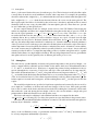
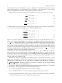
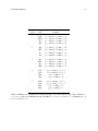
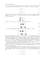
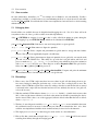
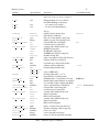
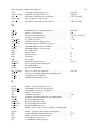
The fluxes and state variables passed between the sea ice model and the CCSM flux coupler are listed
in Table 1. By convention, directional fluxes are positive downward.
The ice fraction ai (aice)1 is the total fractional ice coverage of a grid cell. That is, in each cell,
ai = 0
if there is no ice
ai = 1
if there is no open water
0 < ai < 1 if there is both ice and open water,
1
Typewritten equivalents used in the code are described in the index.
4
Coupling with other climate model components
z◦
~a
U
Qa
ρa
Θa
Ta
Fsw ↓
FL↓
Frain
Fsnow
~τa
Fs
Fl
FL↑
Fevap
α
Tsfc
Atmosphere
Ocean
Provided by the flux coupler to the sea ice model
Atmosphere level height
Ffrzmlt Freezing/melting potential
Wind velocity
Tw
Sea surface temperature
Specific humidity
S
Sea surface salinity
Air density
∇H◦
Sea surface slope
~w
Air potential temperature
U
Surface ocean currents
Air temperature
Shortwave radiation (4 bands)
Incoming longwave radiation
Rainfall rate
Snowfall rate
Provided by the sea ice model to the flux coupler
Wind stress
Fsw ⇓
Penetrating shortwave
Sensible heat flux
Fwater Fresh water flux
Latent heat flux
Fhocn
Net heat flux to ocean
Outgoing longwave
Fsalt
Salt flux
Evaporated water
~τw
Ice-ocean stress
Surface albedo (4 bands)
Surface temperature
ai Ice fraction
Taref 2 m reference temperature (diagnostic)
Qref
2 m reference humidity (diagnostic)
a
Fswabs Absorbed shortwave (diagnostic)
Table 1: Data exchanged between the CCSM flux coupler and the sea ice model.
2.1
Atmosphere
5
where ai is the sum of fractional ice areas for each category of ice. The ice fraction is used by the flux coupler
to merge fluxes from the ice model with fluxes from the other components. For example, the penetrating
shortwave radiation flux, weighted by ai , is combined with the net shortwave radiation flux through ice-free
leads, weighted by (1 − ai ), to obtain the net shortwave flux into the ocean over the entire grid cell. The
flux coupler requires the fluxes to be divided by the total ice area so that the ice and land models are treated
identically (land also may occupy less than 100% of an atmospheric grid cell). These fluxes are “per unit
ice area” rather than “per unit grid cell area.”
In some coupled climate models (for example, recent versions of the U.K. Hadley Centre model) the
surface air temperature and fluxes are computed within the atmosphere model and are passed to CICE. In
this case the logical parameter calc Tsfc in ice therm vertical is set to false. The fields fsurfn (the
net surface heat flux from the atmosphere), flatn (the surface latent heat flux), and fcondtopn (the
conductive flux at the top surface) for each ice thickness category are copied or derived from the input
coupler fluxes and are passed to the thermodynamic driver subroutine, thermo vertical. At the end of the
time step, the surface temperature and effective conductivity (i.e., thermal conductivity divided by thickness)
of the top ice/snow layer in each category are returned to the atmosphere model via the coupler. Since the ice
surface temperature is treated explicitly, the effective conductivity may need to be limited to ensure stability.
As a result, accuracy may be significantly reduced, especially for thin ice or snow layers. A more stable and
accurate procedure would be to compute the temperature profiles for both the atmosphere and ice, together
with the surface fluxes, in a single implicit calculation. This was judged impractical, however, given that the
atmosphere and sea ice models generally exist on different grids and/or processor sets.
2.1
Atmosphere
The wind velocity, specific humidity, air density and potential temperature at the given level height z◦ are
used to compute transfer coefficients used in formulas for the surface wind stress and turbulent heat fluxes
~τa , Fs , and Fl , as described below. Wind stress is arguably the primary forcing mechanism for the ice
motion, although the ice–ocean stress, Coriolis force, and slope of the ocean surface are also important [41].
The sensible and latent heat fluxes, Fs and Fl , along with shortwave and longwave radiation, Fsw ↓ , FL↓ and
FL↑ , are included in the flux balance that determines the ice or snow surface temperature when calc Tsfc
= true. As described in Section 3.5, these fluxes depend nonlinearly on the ice surface temperature Tsfc . The
balance equation is iterated until convergence, and the resulting fluxes and Tsfc are then passed to the flux
coupler.
The snowfall precipitation rate (provided as liquid water equivalent and converted by the ice model to
snow depth) also contributes to the heat and water mass budgets of the ice layer. Melt ponds generally
form on the ice surface in the Arctic and refreeze later in the fall, reducing the total amount of fresh water
that reaches the ocean and altering the heat budget of the ice; this version includes a simple melt pond
parameterization. Rain and all melted snow end up in the ocean.
Wind stress and transfer coefficients for the turbulent heat fluxes are computed in subroutine
atmo boundary layer following [22]. For clarity, the equations are reproduced here in the present notation.
The wind stress and turbulent heat flux calculation accounts for both stable and unstable atmosphere-ice
boundary layers. Define the “stability”
κgz◦
Υ = ∗2
u
Θ∗
Q∗
+
,
Θa (1 + 0.606Qa ) 1/0.606 + Qa
where κ is the von Karman constant, g is gravitational acceleration, and u∗ , Θ∗ and Q∗ are turbulent scales
for velocity, temperature and humidity, respectively:
~ u∗ = cu U
a
6
Coupling with other climate model components
Θ∗ = cθ (Θa − Tsfc )
∗
Q
(1)
= cq (Qa − Qsfc ) .
The wind speed has a minimum value of 1 m/s. We have ignored ice motion in u∗ , and Tsfc and Qsfc are
the surface temperature and specific humidity, respectively. The latter is calculated by assuming a saturated
surface, as described in Section 3.5.1.
The exchange coefficients cu , cθ and cq are initialized as
κ
ln(zref /zice )
and updated during a short iteration, as they depend upon the turbulent scales. Here, zref is a reference
height of 10 m and zice is the roughness length scale for the given sea ice category. Υ is constrained to have
magnitude less than 10. Further, defining χ = (1 − 16Υ)0.25 and χ ≥ 1, the “integrated flux profiles” for
momentum and stability in the unstable (Υ < 0) case are given by
ψm =
ψs =
h
i
2 ln [0.5(1 + χ)] + ln 0.5(1 + χ2 ) − 2 tan−1 χ +
h
π
,
2
i
2 ln 0.5(1 + χ2 ) .
In a departure from the parameterization used in [22], we use profiles for the stable case following [21],
ψm = ψs = − [0.7Υ + 0.75 (Υ − 14.3) exp (−0.35Υ) + 10.7] .
The coefficients are then updated as
cu
1 + cu (λ − ψm ) /κ
cθ
=
1 + cθ (λ − ψs ) /κ
= c0θ
c0u =
c0θ
c0q
where λ = ln (z◦ /zref ). The first iteration ends with new turbulent scales from equations (1). After five
iterations the latent and sensible heat flux coefficients are computed, along with the wind stress:
Cl = ρa (Lvap + Lice ) u∗ cq
Cs = ρa cp u∗ c∗θ + 1,
~a
ρa u∗2 U
~τa =
,
~ a|
|U
where Lvap and Lice are latent heats of vaporization and fusion, ρa is the density of air and cp is its specific
heat. Again following [21], we have added a constant to the sensible heat flux coefficient in order to allow
some heat to pass between the atmosphere and the ice surface in stable, calm conditions.
The atmospheric reference temperature Taref is computed from Ta and Tsfc using the coefficients cu ,
cθ and cq . Although the sea ice model does not use this quantity, it is convenient for the ice model to
perform this calculation. The atmospheric reference temperature is returned to the flux coupler as a climate
diagnostic. The same is true for the reference humidity, Qref
a .
Additional details about the latent and sensible heat fluxes and other quantities referred to here can be
found in Section 3.5.1.
2.2
Ocean
2.2
Ocean
7
New sea ice forms when the ocean temperature drops below its freezing temperature, Tf = −µS, where S
is the seawater salinity and µ = 0.054 ◦ /psu is the ratio of the freezing temperature of brine to its salinity.
The ocean model performs this calculation; if the freezing/melting potential Ffrzmlt is positive, its value
represents a certain amount of frazil ice that has formed in one or more layers of the ocean and floated to the
surface. (The ocean model assumes that the amount of new ice implied by the freezing potential actually
forms.) In general, this ice is added to the thinnest ice category. The new ice is grown in the open water area
of the grid cell to a specified minimum thickness; if the open water area is nearly zero or if there is more
new ice than will fit into the thinnest ice category, then the new ice is spread over the entire cell.
If Ffrzmlt is negative, it is used to heat already existing ice from below. In particular, the sea surface
temperature and salinity are used to compute an oceanic heat flux Fw (|Fw | ≤ |Ffrzmlt |) which is applied at
the bottom of the ice. The portion of the melting potential actually used to melt ice is returned to the coupler
in Fhocn . The ocean model adjusts its own heat budget with this quantity, assuming that the rest of the flux
remained in the ocean.
In addition to runoff from rain and melted snow, the fresh water flux Fwater includes ice meltwater
from the top surface and water frozen (a negative flux) or melted at the bottom surface of the ice. This
flux is computed as the net change of fresh water in the ice and snow volume over the coupling time step,
excluding frazil ice formation and newly accumulated snow. Setting the namelist option update ocn f to
true causes frazil ice to be included in the fresh water and salt fluxes.
There is a flux of salt into the ocean under melting conditions, and a (negative) flux when sea water is
freezing. However, melting sea ice ultimately freshens the top ocean layer, since the ocean is much more
saline than the ice. The ice model passes the net flux of salt Fsalt to the flux coupler, based on the net change
in salt for ice in all categories. In the present configuration, ice ref salinity is used for computing
the salt flux, although the ice salinity used in the thermodynamic calculation has differing values in the ice
layers.
A fraction of the incoming shortwave Fsw ⇓ penetrates the snow and ice layers and passes into the ocean,
as described in Section 3.5.1.
Many ice models compute the sea surface slope ∇H◦ from geostrophic ocean currents provided by an
ocean model or other data source. In our case, the sea surface height H◦ is a prognostic variable in POP—the
flux coupler can provide the surface slope directly, rather than inferring it from the currents. (The option of
computing it from the currents is provided in subroutine evp prep.) The sea ice model uses the surface layer
~ w to determine the stress between the ocean and the ice, and subsequently the ice velocity ~u. This
currents U
stress, relative to the ice,
h
~
~τw = cw ρw U
u
w −~
~ w − ~u cos θ + k̂ × U
~ w − ~u sin θ
U
i
is then passed to the flux coupler (relative to the ocean) for use by the ocean model. Here, θ is the turning
angle between geostrophic and surface currents, cw is the ocean drag coefficient, ρw is the density of seawater (dragw = cw ρw ), and k̂ is the vertical unit vector. The turning angle is necessary if the top ocean model
layers are not able to resolve the Ekman spiral in the boundary layer. If the top layer is sufficiently thin
compared to the typical depth of the Ekman spiral, then θ = 0 is a good approximation. Here we assume
that the top layer is thin enough.
3
Model components
The Arctic and Antarctic sea ice packs are mixtures of open water, thin first-year ice, thicker multiyear ice,
and thick pressure ridges. The thermodynamic and dynamic properties of the ice pack depend on how much
8
Model components
distribution
kcatbound
NC
category
1
2
3
4
5
6
7
original
0
5
0.00
0.64
1.39
2.47
4.57
round
WMO
1
2
5
5
6
lower bound (m)
0.00 0.00 0.00
0.60 0.30 0.15
1.40 0.70 0.30
2.40 1.20 0.70
3.60 2.00 1.20
2.00
7
0.00
0.10
0.15
0.30
0.70
1.20
2.00
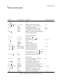
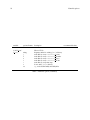
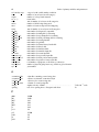
Table 2: Lower boundary values for thickness categories, in meters, for the three distribution options
(kcatbound). In the WMO case, the distribution used depends on the number of categories used.
ice lies in each thickness range. Thus the basic problem in sea ice modeling is to describe the evolution of
the ice thickness distribution (ITD) in time and space.
The fundamental equation solved by CICE is [43]:
∂g
∂
= −∇ · (gu) −
(f g) + ψ,
∂t
∂h
(2)
∂
∂
where u is the horizontal ice velocity, ∇ = ( ∂x
, ∂y
), f is the rate of thermodynamic ice growth, ψ is a
ridging redistribution function, and g is the ice thickness distribution function. We define g(x, h, t) dh as
the fractional area covered by ice in the thickness range (h, h + dh) at a given time and location.
Equation (2) is solved by partitioning the ice pack in each grid cell into discrete thickness categories.
The number of categories can be set by the user, with a default value NC = 5. (Five categories, plus open
water, are generally sufficient to simulate the annual cycles of ice thickness, ice strength, and surface fluxes
[3, 24].) Each category n has lower thickness bound Hn−1 and upper bound Hn . The lower bound of the
thinnest ice category, H0 , is set to zero. The other boundaries are chosen with greater resolution for small
h, since the properties of the ice pack are especially sensitive to the amount of thin ice [28]. The continuous
function g(h) is replaced by the discrete variable ain , defined as the fractional area covered by ice in the
P C
thickness range (Hn−1 , Hn ). We denote the fractional area of open water by ai0 , giving N
n=0 ain = 1 by
definition.
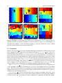
Category boundaries are computed in init itd using one of several formulas, summarized in Table 2.
Setting the namelist variable kcatbound equal to 0 or 1 gives lower thickness boundaries for any number
of thickness categories NC . Table 2 shows the boundary values for NC = 5. A third option specifies
the boundaries based on the World Meteorological Organization classification; the full WMO thickness
distribution is used if NC = 7; if NC = 5 or 6, some of the thinner categories are combined. The original
formula (kcatbound = 0) is the default because it was used to create the restart files included with the
code distribution. Users may substitute their own preferred boundaries in init itd.
In addition to the fractional ice area, ain , we define the following state variables for each category n:
• vin , the ice volume, equal to the product of ain and the ice thickness hin .
• vsn , the snow volume, equal to the product of ain and the snow thickness hsn .
• eink , the internal ice energy in layer k, equal to the product of the ice layer volume, vin /Ni , and the
ice layer enthalpy, qink . Here Ni is the total number of ice layers, with a default value Ni = 4, and
3.1
Horizontal transport
9
qink is the negative of the energy needed to melt a unit volume of ice and raise its temperature to 0◦ C;
it is discussed in Section 3.5. (NOTE: In the current code, ei < 0 and qi < 0 with ei = vi qi .)
• esnk , the internal snow energy in layer k, equal to the product of the snow layer volume, vsn /Ns , and
the snow layer enthalpy, qsnk , where Ns is the number of snow layers. (Similarly, es < 0 in the code.)
Earlier versions of CICE had a single snow layer, but multiple layers are now allowed. The default
value is Ns = 1.
• Tsfn , the surface temperature
• τage , the volume-weighted mean ice age.
Since the fractional area is unitless, the volume variables have units of meters (i.e., m3 of ice or snow per
m2 of grid cell area), and the energy variables have units of J/m2 . Both Tsfn and τage are assigned to the
tracer array trcrn, which consists of Ntr fields. By default, Ntr = 2, but users may create any number of
additional tracer fields.
The three terms on the right-hand side of (2) describe three kinds of sea ice transport: (1) horizontal
transport in (x, y) space; (2) transport in thickness space h due to thermodynamic growth and melting; and
(3) transport in thickness space h due to ridging and other mechanical processes. We solve the equation
by operator splitting in three stages, with two of the three terms on the right set to zero in each stage. We
compute horizontal transport using the incremental remapping scheme of [7] as adapted for sea ice by [25];
this scheme is discussed in Section 3.1. Ice is transported in thickness space using the remapping scheme
of [24], as described in Section 3.2. The mechanical redistribution scheme, based on [43], [35], [14], [11],
and [26], is outlined in Section 3.3. To solve the horizontal transport and ridging equations, we need the
ice velocity u, and to compute transport in thickness space, we must know the the ice growth rate f in each
thickness category. We use the elastic-viscous-plastic (EVP) ice dynamics scheme of [17], as modified by
[6], [15], [18] and [19], to find the velocity, as described in Section 3.4. Finally, we use the thermodynamic
model of [4], discussed in Section 3.5, to compute f .
The order in which these computations are performed in the code itself was chosen so that quantities
sent to the coupler are consistent with each other and as up-to-date as possible. In earlier versions of CICE,
fluxes and state variables were sent to the coupler during the timestep, after initial thermodynamic surface
fluxes had been computed but before the rest of the thermodynamics and dynamics calculations. This was
done to improve load balancing in a concurrent coupling scheme (model components ran simultaneously
rather than sequentially). CCSM no longer requires this and so the coupling is now done at the end of
the timestep, simplifying the code a great deal. However, the Delta-Eddington radiative scheme computes
albedo and shortwave components simultaneously, and in order to have the most up-to-date values available
for the coupler at the end of the timestep, the order of radiation calculations needed to be shifted. Albedo
and shortwave components are computed after the ice state has been modified by both thermodynamics and
dynamics, so that they are consistent with the ice area and thickness at the end of the step when sent to the
coupler. However, they are computed using the downwelling shortwave from the beginning of the timestep.
Rather than recompute the albedo and shortwave components at the beginning of the next timestep using
new values of the downwelling shortwave forcing, the shortwave components computed at the end of the
last timestep are scaled for the new forcing.
3.1
Horizontal transport
We wish to solve the continuity or transport equation,
∂ain
+ ∇ · (ain u) = 0,
∂t
(3)
10
Model components
for the fractional ice area in each thickness category n. Equation (3) describes the conservation of ice area
under horizontal transport. It is obtained from (2) by discretizing g and neglecting the second and third
terms on the right-hand side, which are treated separately (Sections 3.2 and 3.3).
There are similar conservation equations for ice volume, snow volume, ice energy and snow energy:
∂vin
+ ∇ · (vin u)
∂t
∂vsn
+ ∇ · (vsn u)
∂t
∂eink
+ ∇ · (eink u)
∂t
∂esnk
+ ∇ · (esnk u)
∂t
= 0,
(4)
= 0,
(5)
= 0,
(6)
= 0.
(7)
In addition, there are one or more equations describing tracer transport, whose values are contained in the
trcrn array. These equations typically have one of the following three forms
∂ (ain Tn )
+ ∇ · (ain Tn u) = 0,
∂t
∂ (vin Tn )
+ ∇ · (vin Tn u) = 0,
∂t
∂ (vsn Tn )
+ ∇ · (vsn Tn u) = 0.
∂t
(8)
(9)
(10)
Equation (8) describes the transport of surface temperature, whereas (9) and (10) describe the transport of
passive tracers such as volume-weighted ice age and snow age. Each tracer field is given an integer index,
trcr depend, which has the value 0, 1, or 2 depending on whether the appropriate conservation equation
is (8) (9), or (10), respectively. The total number of tracers is Ntr ≥ 1. In the default configuration there
are two tracers: surface temperature and volume-weighted ice age. Tracers for melt pond volume, level ice
area and level ice volume (used to diagnose ridged ice area and volume) are also available. Users may add
any number of additional tracers that are transported conservatively provided that trcr depend is defined
appropriately. See Section 4.8.3 for guidance on adding tracers.
The age of the ice is treated as an ice-area tracer (trcr depend = 0). It is initialized at 0 when ice
forms as frazil, and the ice ages the length of the timestep during each timestep. Freezing directly onto
the bottom of the ice does not affect the age, nor does melting. Mechanical redistribution processes and
advection alter the age of ice in any given grid cell in a conservative manner following changes in ice area.
The sea ice age tracer is validated in [16].
By default, ice and snow are assumed to have constant densities, so that volume conservation is equivalent to mass conservation. Variable-density ice and snow layers can be transported conservatively by
defining tracers corresponding to ice and snow density, as explained in the introductory comments in
ice transport remap.F90. Prognostic equations for ice and/or snow density may be included in future
model versions but have not yet been implemented.
Two transport schemes are available: upwind and the incremental remapping scheme of [7] as modified
for sea ice by [25]. The remapping scheme has several desirable features:
• It conserves the quantity being transported (area, volume, or energy).
• It is non-oscillatory; that is, it does not create spurious ripples in the transported fields.
• It preserves tracer monotonicity. That is, it does not create new extrema in the thickness and enthalpy
fields; the values at time m + 1 are bounded by the values at time m.
Horizontal transport
11
• It is second-order accurate in space and therefore is much less diffusive than first-order schemes (e.g.,
upwind). The accuracy may be reduced locally to first order to preserve monotonicity.
• It is efficient for large numbers of categories or tracers. Much of the work is geometrical and is
performed only once per grid cell instead of being repeated for each quantity being transported.
The time step is limited by the requirement that trajectories projected backward from grid cell corners are
confined to the four surrounding cells; this is what is meant by incremental remapping as opposed to general
remapping. This requirement leads to a CFL-like condition,
max |u|∆t
≤ 1.
∆x
For highly divergent velocity fields the maximum time step must be reduced by a factor of two to ensure
that trajectories do not cross. However, ice velocity fields in climate models usually have small divergences
per time step relative to the grid size.
The remapping algorithm can be summarized as follows:
1. Given mean values of the ice area and tracer fields in each grid cell, construct linear approximations
of these fields. Limit the field gradients to preserve monotonicity.
2. Given ice velocities at grid cell corners, identify departure regions for the fluxes across each cell edge.
Divide these departure regions into triangles and compute the coordinates of the triangle vertices.
3. Integrate the area and tracer fields over the departure triangles to obtain the area, volume, and energy
transported across each cell edge.
4. Given these transports, update the state variables.
Since all scalar fields are transported by the same velocity field, step (2) is done only once per time step.
The other three steps are repeated for each field in each thickness category. These steps are described below.
3.1.1
Reconstructing area and tracer fields
First, using the known values of the state variables, the ice area and tracer fields are reconstructed in each
grid cell as linear functions of x and y. For each field we compute the value at the cell center (i.e., at the
origin of a 2D Cartesian coordinate system defined for that grid cell), along with gradients in the x and
y directions. The gradients are limited to preserve monotonicity. When integrated over a grid cell, the
reconstructed fields must have mean values equal to the known state variables, denoted by ā for fractional
area, h̃ for thickness, and q̂ for enthalpy. The mean values are not, in general, equal to the values at the cell
center. For example, the mean ice area must equal the value at the centroid, which may not lie at the cell
center.
Consider first the fractional ice area, the analog to fluid density ρ in [7]. For each thickness category we
construct a field a(r) whose mean is ā, where r = (x, y) is the position vector relative to the cell center.
That is, we require
Z
a dA = ā A,
(11)
A
where A =
R
A dA
is the grid cell area. Equation (11) is satisfied if a(r) has the form
a(r) = ā + αa h∇ai · (r − r̄),
(12)
12
Model components
where h∇ai is a centered estimate of the area gradient within the cell, αa is a limiting coefficient that
enforces monotonicity, and r̄ is the cell centroid:
r̄ =
1
A
Z
r dA.
A
It follows from (12) that the ice area at the cell center (r = 0) is
ac = ā − ax x − ay y,
where ax = αa (∂a/∂x) and ay = αa (∂a/∂y)
are the limitedR gradients in the x and y directions, respecR
tively, and the components of r̄, x = A x dA/A and y = A y dA/A, are evaluated using the triangle
integration formulas described in Section 3.1.3. These means, along with higher-order means such as x2 ,
xy, and y 2 , are computed once and stored.
Next consider the ice and snow thickness and enthalpy fields. Thickness is analogous to the tracer
concentration T in [7], but there is no analog in [7] to the enthalpy. The reconstructed ice or snow thickness
h(r) and enthalpy q(r) must satisfy
Z
a h dA = ā h̃ A,
(13)
a h q dA = ā h̃ q̂ A,
(14)
Z A
A
where h̃ = h(r̃) is the thickness at the center of ice area, and q̂ = q(r̂) is the enthalpy at the center of ice or
snow volume. Equations (13) and (14) are satisfied when h(r) and q(r) are given by
h(r) = h̃ + αh h∇hi · (r − r̃),
(15)
q(r) = q̂ + αq h∇qi · (r − r̂),
(16)
where αh and αq are limiting coefficients. The center of ice area, r̃, and the center of ice or snow volume,
r̂, are given by
Z
1
r̃ =
a r dA,
ā A A
1
a h r dA.
ā h̃ A A
Evaluating the integrals, we find that the components of r̃ are
Z
r̂ =
x̃ =
ac x + ax x2 + ay xy
,
ā
ỹ =
ac y + ax xy + ay y 2
,
ā
and the components of r̂ are
x̂ =
c1 x + c2 x2 + c3 xy + c4 x3 + c5 x2 y + c6 xy 2
,
ā h̃
ŷ =
c1 y + c2 xy + c3 y 2 + c4 x2 y + c5 xy 2 + c6 y 3
,
ā h̃
Horizontal transport
13
where
c1 ≡ ac hc ,
c2 ≡ ac hx + ax hc ,
c3 ≡ ac hy + ay hc ,
c4 ≡ ax hx ,
c5 ≡ ax hy + ay hx ,
c6 ≡ ay hy .
From (15) and (16), the thickness and enthalpy at the cell center are given by
hc = h̃ − hx x̃ − hy ỹ,
qc = q̂ − qx x̂ − qy ŷ,
where hx , hy , qx and qy are the limited gradients of thickness and enthalpy. The surface temperature is
treated the same way as ice or snow thickness, but it has no associated enthalpy. Tracers obeying conservation equations of the form (9) and (10) are treated in analogy to ice and snow enthalpy, respectively.
We preserve monotonicity by van Leer limiting. If φ̄(i, j) denotes the mean value of some field in grid
cell (i, j), we first compute centered gradients of φ̄ in the x and y directions, then check whether these
gradients give values of φ within cell (i, j) that lie outside the range of φ̄ in the cell and its eight neighbors.
Let φ̄max and φ̄min be the maximum and minimum values of φ̄ over the cell and its neighbors, and let
φmax and φmin be the maximum and minimum values of the reconstructed φ within the cell. Since the
reconstruction is linear, φmax and φmin are located at cell corners. If φmax > φ̄max or φmin < φ̄min , we
multiply the unlimited gradient by α = min(αmax , αmin ), where
αmax = (φ̄max − φ̄)/(φmax − φ̄),
αmin = (φ̄min − φ̄)/(φmin − φ̄).
Otherwise the gradient need not be limited.
Earlier versions of CICE (through 3.14) computed gradients in physical space. In version 4.0, gradients
are computed in a scaled space in which each grid cell has sides of unit length. The origin is at the cell
center, and the four vertices are located at (0.5, 0.5), (-0.5,0.5),(-0.5, -0.5) and (0.5, -0.5). In this coordinate
system, several of the above grid-cell-mean quantities vanish (because they are odd functions of x and/or y),
but they have been retained in the code for generality.
3.1.2
Locating departure triangles
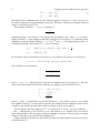
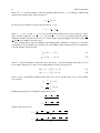
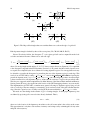
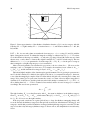
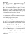
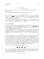
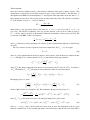
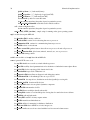
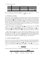
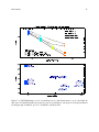
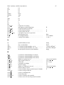
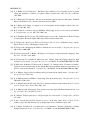
The method for locating departure triangles is discussed in detail by [7]. The basic idea is illustrated in
Figure 1, which shows a shaded quadrilateral departure region whose contents are transported to the target or
home grid cell, labeled H. The neighboring grid cells are labeled by compass directions: N W , N , N E, W ,
and E. The four vectors point along the velocity field at the cell corners, and the departure region is formed
by joining the starting points of these vectors. Instead of integrating over the entire departure region, it is
convenient to compute fluxes across cell edges. We identify departure regions for the north and east edges of
each cell, which are also the south and west edges of neighboring cells. Consider the north edge of the home
cell, across which there are fluxes from the neighboring N W and N cells. The contributing region from the
N W cell is a triangle with vertices abc, and that from the N cell is a quadrilateral that can be divided into two
triangles with vertices acd and ade. Focusing on triangle abc, we first determine the coordinates of vertices
14
Model components
Figure 1: In incremental remapping, conserved quantities are remapped from the shaded departure region,
a quadrilateral formed by connecting the backward trajectories from the four cell corners, to the grid cell
labeled H. The region fluxed across the north edge of cell H consists of a triangle (abc) in the N W cell and
a quadrilateral (two triangles, acd and ade) in the N cell.
b and c relative to the cell corner (vertex a), using Euclidean geometry to find vertex c. Then we translate
the three vertices to a coordinate system centered in the N W cell. This translation is needed in order to
integrate fields (Section 3.1.3) in the coordinate system where they have been reconstructed (Section 3.1.1).
Repeating this process for the north and east edges of each grid cell, we compute the vertices of all the
departure triangles associated with each cell edge.
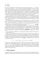
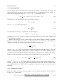
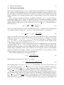
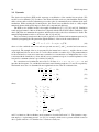
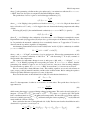
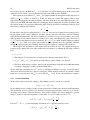
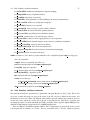
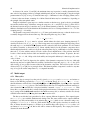
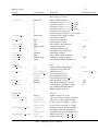
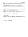
Figure 2, reproduced from [7], shows all possible triangles that can contribute fluxes across the north
edge of a grid cell. There are 20 triangles, which can be organized into five groups of four mutually exclusive triangles as shown in Table 3. In this table, (x1 , y1 ) and (x2 , y2 ) are the Cartesian coordinates of the
departure points relative to the northwest and northeast cell corners, respectively. The departure points are
joined by a straight line that intersects the west edge at (0, ya ) relative to the northwest corner and intersects
the east edge at (0, yb ) relative to the northeast corner. The east cell triangles and selecting conditions are
identical except for a rotation through 90 degrees.
This scheme was originally designed for rectangular grids. Grid cells in CICE actually lie on the surface
of a sphere and must be projected onto a plane. The projection used in CICE 4.0 maps each grid cell to a
square with sides of unit length. Departure triangles across a given cell edge are computed in a coordinate
system whose origin lies at the midpoint of the edge and whose vertices are at (-0.5, 0) and (0.5, 0). Intersection points are computed assuming Cartesian geometry with cell edges meeting at right angles. Let CL
and CR denote the left and right vertices, which are joined by line CLR. Similarly, let DL and DR denote
the departure points, which are joined by line DLR. Also, let IL and IR denote the intersection points (0, ya )
and (0,yb ) respectively, and let IC = (xc , 0) denote the intersection of CLR and DLR. It can be shown that
ya , yb , and xc are given by
xCL (yDM − yDL ) + xDM yDL − xDL yDM
xDM − xDL ,
xCR (yDR − yDM ) − xDM yDR + xDR yDM
=
x
− xDM ,
DR
xDR − xDL
= xDL − yDL
yDR − yDL
ya =
yb
xc
Horizontal transport
15
Triangle
group
Triangle
label
Selecting logical
condition
1
NW
NW1
W
W2
ya
ya
ya
ya
> 0 and y1
< 0 and y1
< 0 and y1
> 0 and y1
≥ 0 and x1
≥ 0 and x1
< 0 and x1
< 0 and x1
<0
<0
<0
<0
2
NE
NE1
E
E2
yb
yb
yb
yb
> 0 and y2
< 0 and y2
< 0 and y2
> 0 and y2
≥ 0 and x2
≥ 0 and x2
< 0 and x2
< 0 and x2
>0
>0
>0
>0
3
W1
NW2
E1
NE2
ya < 0 and y1 ≥ 0 and x1 < 0
ya > 0 and y1 < 0 and x1 < 0
yb < 0 and y2 ≥ 0 and x2 > 0
yb > 0 and y2 < 0 and x2 > 0
4
H1a
N1a
H1b
N1b
ya yb ≥ 0 and ya + yb < 0
ya yb ≥ 0 and ya + yb > 0
ya yb < 0 and ỹ1 < 0
ya yb < 0 and ỹ1 > 0
5
H2a
N2a
H2b
N2b
ya yb ≥ 0 and ya + yb < 0
ya yb ≥ 0 and ya + yb > 0
ya yb < 0 and ỹ2 < 0
ya yb < 0 and ỹ2 > 0
Table 3: Evaluation of contributions from the 20 triangles across the north cell edge. The coordinates x1 ,
x2 , y1 , y2 , ya , and yb are defined in the text. We define ỹ1 = y1 if x1 > 0, else ỹ1 = ya . Similarly, ỹ2 = y2
if x2 < 0, else ỹ2 = yb .
16
Model components
N
NW
NW
W
1
W
N
2
Home
NE
NW
NE
E
E
NE
N2a
1
N1a
2
H1a
W
E
H2a
Home
(a)
(b)
N
NE
NW
1
N1b
H1b
N2b
H2b
W
2
E
Home
(c)
NW
W
1
NW1
W1
N
2
Home
NE1
E1
NE
NW
E
W
(d1)
NW2
1
N
2
NE2
NE
E2
W2
Home
E
(d2)
Figure 2: The 20 possible triangles that can contribute fluxes across the north edge of a grid cell.
Each departure triangle is defined by three of the seven points (CL, CR, DL, DR, IL, IR, IC).
Given a 2D velocity field u , the divergence ∇ · u in a given grid cell can be computed from the local
velocities and written in terms of fluxes across each cell edge:
1
∇·u=
A
uN E + uSE
2
LE +
uN W + uSW
2
LW +
uN E + uN W
2
LN +
uSE + uSW
2
LS ,
(17)
where L is an edge length and the indices N, S, E, W denote compass directions. Equation (17) is equivalent
to the divergence computed in the EVP dynamics (Section 3.4). In general, the fluxes in this expression are
not equal to those implied by the above scheme for locating departure regions. For some applications it may
be desirable to prescribe the divergence by prescribing the area of the departure region for each edge. This
can be done in CICE 4.0 by setting l fixed area = true in ice transport driver.F90 and passing the
prescribed departure areas (edgearea e and edgearea n) into the remapping routine. An extra triangle
is then constructed for each departure region to ensure that the total area is equal to the prescribed value.
This idea was suggested and first implemented by Mats Bentsen of the Nansen Environmental and Remote
Sensing Center (Norway), who applied an earlier version of the CICE remapping scheme to an ocean model.
The implementation in CICE 4.0 is somewhat more general, allowing for departure regions lying on both
sides of a cell edge. The extra triangle is constrained to lie in one but not both of the grid cells that share the
edge. Since this option has yet to be fully tested in CICE, the current default is l fixed area = false.
We made one other change in the scheme of [7] for locating triangles. In their paper, departure points
are defined by projecting cell corner velocities directly backward. That is,
xD = −u ∆t,
(18)
where xD is the location of the departure point relative to the cell corner and u is the velocity at the corner.
This approximation is only first-order accurate. Accuracy can be improved by estimating the velocity at the
midpoint of the trajectory.
Horizontal transport
3.1.3
17
Integrating fields
Next, we integrate the reconstructed fields over the departure triangles to find the total area, volume, and
energy transported across each cell edge. Area transports are easy to compute since the area is linear in x
and y. Given a triangle with vertices xi = (xi , yi ), i ∈ {1, 2, 3}, the triangle area is
AT =
1
|(x2 − x1 )(y3 − y1 ) − (y2 − y1 )(x3 − x1 )| .
2
(19)
The integral Fa of any linear function f (r) over a triangle is given by
Fa = AT f (x0 ),
(20)
3
1X
xi .
x0 =
3 i=1
(21)
where x0 = (x0 , y0 ) is the triangle midpoint,
To compute the area transport, we evaluate the area at the midpoint,
a(x0 ) = ac + ax x0 + ay y0 ,
(22)
and multiply by AT . By convention, northward and eastward transport is positive, while southward and
westward transport is negative.
Equation (20) cannot be used for volume transport, because the reconstructed volumes are quadratic
functions of position. (They are products of two linear functions, area and thickness.) The integral of a
quadratic polynomial over a triangle requires function evaluations at three points,
Fh =
3
AT X
f x0i ,
3 i=1
(23)
where x0i = (x0 + xi )/2 are points lying halfway between the midpoint and the three vertices. [7] use this
formula to compute transports of the product ρ T , which is analogous to ice volume. Equation (23) does
not work for ice and snow energies, which are cubic functions—products of area, thickness, and enthalpy.
Integrals of a cubic polynomial over a triangle can be evaluated using a four-point formula [42]:
"
F q = AT
3
9
25 X
− f (x0 ) +
f (x00i )
16
48 i=1
#
(24)
where xi 00 = (3x0 + 2xi )/5. To evaluate functions at specific points, we must compute many products of
the form a(x) h(x) and a(x) h(x) q(x), where each term in the product is the sum of a cell-center value
and two displacement terms. In the code, the computation is sped up by storing some sums that are used
repeatedly.
3.1.4
Updating state variables
Finally, we compute new values of the state variables in each ice category and grid cell. The new fractional
ice areas a0in (i, j) are given by
a0in (i, j) = ain (i, j) +
FaE (i − 1, j) − FaE (i, j) + FaN (i, j − 1) − FaN (i, j)
A(i, j)
(25)
18
Model components
where FaE (i, j) and FaN (i, j) are the area transports across the east and north edges, respectively, of cell
(i, j), and A(i, j) is the grid cell area. All transports added to one cell are subtracted from a neighboring
cell; thus (25) conserves total ice area.
The new ice volumes and energies are computed analogously. New thicknesses are given by the ratio of
volume to area, and enthalpies by the ratio of energy to volume. Tracer monotonicity is ensured because
R
a h dA
h = RA
,
0
A a dA
R
a h q dA
q = RA
,
0
Aah
dA
where h0 and q 0 are the new-time thickness and enthalpy, given by integrating the old-time ice area, volume,
and energy over a Lagrangian departure region with area A. That is, the new-time thickness and enthalpy
are weighted averages over old-time values, with non-negative weights a and ah. Thus the new-time values
must lie between the maximum and minimum of the old-time values.
3.2
Transport in thickness space
Next we solve the equation for ice transport in thickness space due to thermodynamic growth and melt,
∂
∂g
+
(f g) = 0,
(26)
∂t
∂h
which is obtained from (2) by neglecting the first and third terms on the right-hand side. We use the remapping method of [24], in which thickness categories are represented as Lagrangian grid cells whose boundaries are projected forward in time. The thickness distribution function g is approximated as a linear function
of h in each displaced category and is then remapped onto the original thickness categories. This method is
numerically smooth and is not too diffusive. It can be viewed as a 1D simplification of the 2D incremental
remapping scheme described above.
We first compute the displacement of category boundaries in thickness space. Assume that at time m
m
the ice areas am
n and mean ice thicknesses hn are known for each thickness category. (For now we omit
the subscript i that distinguishes ice from snow.) We use a thermodynamic model (Section 3.5) to compute
at time m + 1. The time step must be small enough that trajectories do
the new mean thicknesses hm+1
n
m+1
not cross; i.e., hm+1
<
h
for
each pair of adjacent categories. The growth rate at h = hn is given
n
n+1
m+1
m
by fn = (hn
− hn )/∆t. By linear interpolation we estimate the growth rate Fn at the upper category
boundary Hn :
fn+1 − fn
Fn = fn +
(Hn − hn ).
hn+1 − hn
If an or an+1 = 0, Fn is set to the growth rate in the nonzero category, and if an = an+1 = 0, we set
Fn = 0. The temporary displaced boundaries are given by
Hn∗ = Hn + Fn ∆t, n = 1 to N − 1
The boundaries must not be displaced by more than one category to the left or right; that is, we require
Hn−1 < Hn∗ < Hn+1 . Without this requirement we would need to do a general remapping rather than an
incremental remapping, at the cost of added complexity.
Next we construct g(h) in the displaced thickness categories. The ice areas in the displaced categories
are am+1
= am
n
n , since area is conserved following the motion in thickness space (i.e., during vertical ice
m+1 . For conciseness, define
growth or melting). The new ice volumes are vnm+1 = (an hn )m+1 = am
n hn
Transport in thickness space
19
∗
HL = Hn−1
and HR = Hn∗ and drop the time index m + 1. We wish to construct a continuous function
g(h) within each category such that the total area and volume at time m + 1 are an and vn , respectively:
Z HR
g dh = an ,
(27)
h g dh = vn .
(28)
HL
Z HR
HL
The simplest polynomial that can satisfy both equations is a line. It is convenient to change coordinates,
writing g(η) = g1 η + g0 , where η = h − HL and the coefficients g0 and g1 are to be determined. Then (27)
and (28) can be written as
η2
g1 R + g0 ηR = an ,
2
3
η2
ηR
+ g0 R = an ηn ,
3
2
where ηR = HR − HL and ηn = hn − HL . These equations have the solution
g1
6an
g0 = 2
ηR
2ηR
− ηn ,
3
(29)
12an
ηR
.
ηn −
3
2
ηR
(30)
g1 =
Since g is linear, its maximum and minimum values lie at the boundaries, η = 0 and ηR :
6an
g(0) = 2
ηR
g(ηR ) =
2ηR
− η n = g0 ,
3
6an
2
ηR
ηR
.
3
(31)
ηn −
(32)
Equation (31) implies that g(0) < 0 when ηn > 2ηR /3, i.e., when hn lies in the right third of the thickness
range (HL , HR ). Similarly, (32) implies that g(ηR ) < 0 when ηn < ηR /3, i.e., when hn is in the left third
of the range. Since negative values of g are unphysical, a different solution is needed when hn lies outside
the central third of the thickness range. If hn is in the left third of the range, we define a cutoff thickness,
HC = 3hn − 2HL , and set g = 0 between HC and HR . Equations (29) and (30) are then valid with ηR
redefined as HC − HL . And if hn is in the right third of the range, we define HC = 3hn − 2HR and set
g = 0 between HL and HC . In this case, (29) and (30) apply with ηR = HR − HC and ηn = hn − HC .
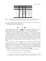
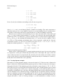
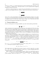
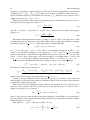
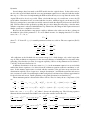
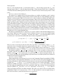
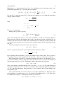
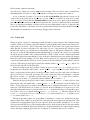
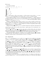
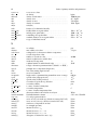
Figure 3 illustrates the linear reconstruction of g for the simple cases HL = 0, HR = 1, an = 1, and
hn = 0.2, 0.4, 0.6, and 0.8. Note that g slopes downward (g1 < 0) when hn is less than the midpoint
thickness, (HL + HR )/2 = 1/2, and upward when hn exceeds the midpoint thickness. For hn = 0.2 and
0.8, g = 0 over part of the range.
Finally, we remap the thickness distribution to the original boundaries by transferring area and volume
between categories. We compute the ice area ∆an and volume ∆vn between each original boundary Hn and
displaced boundary Hn∗ . If Hn∗ > Hn , ice moves from category n to n + 1. The area and volume transferred
are
Z ∗
∆an =
Hn
g dh,
(33)
h g dh.
(34)
Hn
∆vn =
Z H∗
n
Hn
20
Model components
3.5
3.0
h = 0.2
h = 0.4
h = 0.6
h = 0.8
2.5
g(h)
2.0
1.5
1.0
0.5
0.0
0
0.2
0.4
0.6
0.8
1
Ice thickness
Figure 3: Linear approximation of the thickness distribution function g(h) for an ice category with left
boundary HL = 0, right boundary HR = 1, fractional area an = 1, and mean ice thickness hn = 0.2, 0.4,
0.6, and 0.8.
If Hn∗ < HN , ice area and volume are transferred from category n + 1 to n using (33) and (34) with the
limits of integration reversed. To evaluate the integrals we change coordinates from h to η = h − HL , where
HL is the left limit of the range over which g > 0, and write g(η) using (29) and (30). In this way we obtain
the new areas an and volumes vn between the original boundaries Hn−1 and Hn in each category. The new
thicknesses, hn = vn /an , are guaranteed to lie in the range (Hn−1 , Hn ). If g = 0 in the part of a category
that is remapped to a neighboring category, no ice is transferred.
Other conserved quantities are transferred in proportion to the ice volume ∆vin . (We now use the
subscripts i and s to distinguish ice from snow.) For example, the transferred snow volume is ∆vsn =
vsn (∆vin /vin ), and the transferred ice energy in layer k is ∆eink = eink (∆vin /vin ).
The left and right boundaries of the domain require special treatment. If ice is growing in open water at a
rate F0 , the left boundary H0 is shifted to the right by F0 ∆t before g is constructed in category 1, then reset
to zero after the remapping is complete. New ice is then added to the grid cell, conserving area, volume, and
energy. If ice cannot grow in open water (because the ocean is too warm or the net surface energy flux is
downward), H0 is fixed at zero, and the growth rate at the left boundary is estimated as F0 = f1 . If F0 < 0,
all ice thinner than ∆h0 = −F0 ∆t is assumed to have melted, and the ice area in category 1 is reduced
accordingly. The area of new open water is
Z ∆h0
∆a0 =
g dh.
0
The right boundary HN is not fixed but varies with hN , the mean ice thickness in the thickest category.
Given hN , we set HN = 3hN − 2HN −1 , which ensures that g(h) > 0 for HN −1 < h < HN and g(h) = 0
for h ≥ HN . No ice crosses the right boundary.
If the ice growth or melt rates in a given grid cell are too large, the thickness remapping scheme will
not work. Instead, the thickness categories in that grid cell are treated as delta functions following [3], and
categories outside their prescribed boundaries are merged with neighboring categories as needed. For time
steps of less than a day and category thickness ranges of 10 cm or more, this simplification is needed rarely,
if ever.
3.3
Mechanical redistribution
21
3.3
Mechanical redistribution
The last term on the right-hand side of (2) is ψ, which describes the redistribution of ice in thickness space
due to ridging and other mechanical processes. The mechanical redistribution scheme in CICE is based on
[43], [35], [14], [11], and [26]. This scheme converts thinner ice to thicker ice and is applied after horizontal
transport. When the ice is converging, enough ice ridges to ensure that the ice area does not exceed the grid
cell area.
First we specify the participation function: the thickness distribution aP (h) = b(h) g(h) of the ice
participating in ridging. (We use “ridging” as shorthand for all forms of mechanical redistribution, including
rafting.) The weighting function b(h) favors ridging of thin ice and closing of open water in preference to
ridging of thicker ice. There are two options for the form of b(h). If krdg partic = 0 in the namelist, we
follow [43] and set
(
G(h)
2
∗
G∗ (1 − G∗ ) if G(h) < G
b(h) =
(35)
0
otherwise
where G(h) is the fractional area covered by ice thinner than h, and G∗ is an empirical constant. Integrating
aP (h) between category boundaries Hn−1 and Hn , we obtain the mean value of aP in category n:
Gn−1 + Gn
2
(Gn − Gn−1 ) 1 −
,
∗
G
2G∗
aP n =
(36)
where aP n is the ratio of the ice area ridging (or open water area closing) in category n to the total area
ridging and closing, and Gn is the total fractional ice area in categories 0 to n. Equation (36) applies
to categories with Gn < G∗ . If Gn−1 < G∗ < Gn , then (36) is valid with G∗ replacing Gn , and if
Gn−1 > G∗ , then aP n = 0. If the open water fraction a0 > G∗ , no ice can ridge, because “ridging” simply
reduces the area of open water. As in [43] we set G∗ = 0.15.
If the spatial resolution is too fine for a given time step ∆t, the weighting function (35) can promote
numerical instability. For ∆t = 1 hour, resolutions finer than ∆x ∼ 10 km are typically unstable. The
instability results from feedback between the ridging scheme and the dynamics via the ice strength. If the
strength changes significantly on time scales less than ∆t, the viscous-plastic solution of the momentum
equation is inaccurate and sometimes oscillatory. As a result, the fields of ice area, thickness, velocity,
strength, divergence, and shear can become noisy and unphysical.
A more stable weighting function was suggested by [26]:
b(h) =
exp[−G(h)/a∗ ]
a∗ [1 − exp(−1/a∗ )]
(37)
When integrated between category boundaries, (37) implies
aP n =
exp(−Gn−1 /a∗ ) − exp(−Gn /a∗ )
1 − exp(−1/a∗ )
(38)
This weighting function is used if krdg partic = 1 in the namelist. From (37), the mean value of G
for ice participating in ridging is a∗ , as compared to G∗ /3 for (35). For typical ice thickness distributions,
setting a∗ = 0.05 with krdg partic = 1 gives participation fractions similar to those given by G∗ = 0.15
with krdg partic = 0. See [26] for a detailed comparison of these two participation functions.
Thin ice is converted to thick, ridged ice in a way that reduces the total ice area while conserving ice volume and internal energy. There are two namelist options for redistributing ice among thickness categories.
If krdg redist = 0, ridging
is distributed uniformly between
√ice∗ of thickness hn forms ridges whose area
∗
Hmin = 2hn and Hmax = 2 H hn , as in [14]. The default value of H is 25 m, as in earlier versions of
CICE. Observations suggest that H ∗ = 50 m gives a better fit to first-year ridges [1], although the lower
22
Model components
value may be appropriate for multiyear ridges [11]. The ratio of the mean ridge thickness to the thickness
of ridging ice is kn = (Hmin + Hmax )/(2hn ). If the area of category n is reduced by ridging at the rate rn ,
the area of thicker categories grows simultaneously at the rate rn /kn . Thus the net rate of area loss due to
ridging of ice in category n is rn (1 − 1/kn ).
The ridged ice area and volume are apportioned among categories in the thickness range (Hmin , Hmax ).
The fraction of the new ridge area in category m is
area
fm
=
HR − HL
,
Hmax − Hmin
(39)
where HL = max(Hm−1 , Hmin ) and HR = min(Hm , Hmax ). The fraction of the ridge volume going to
category m is
(HR )2 − (HL )2
vol
fm
=
.
(40)
(Hmax )2 − (Hmin )2
This uniform redistribution function tends to produce too little ice in the 3–5 m range and too much
ice thicker than 10 m [1]. Observations show that the ITD of ridges is better approximated by a negative
exponential. Setting krdg redist = 1 gives ridges with an exponential ITD [26]:
gR (h) ∝ exp[−(h − Hmin )/λ]
(41)
for h ≥ Hmin , with gR (h) = 0 for h < Hmin . Here, λ is an empirical e-folding scale and Hmin = 2hn
1/2
(where hn is the thickness of ridging ice). We assume that λ = µhn , where µ (mu rdg) is a tunable
1/2
parameter with units m1/2 . Thus the mean ridge thickness increases in proportion to hn , as in [14]. The
value µ = 4.0 m1/2 gives λ in the range 1–4 m for most ridged ice. Ice strengths with µ = 4.0 m1/2 and
krdg redist = 1 are roughly comparable to the strengths with H ∗ = 50 m and krdg redist = 0.
From (41) it can be shown that the fractional area going to category m as a result of ridging is
area
fm
= exp[−(Hm−1 − Hmin )/λ] − exp[−(Hm − Hmin )/λ].
(42)
The fractional volume going to category m is
vol
fm
=
(Hm−1 + λ) exp[−(Hm−1 − Hmin )/λ] − (Hm + λ) exp[−(Hm − Hmin )/λ]
.
Hmin + λ
(43)
Equations (42) and (43) replace (39) and (40) when krdg redist = 1.
Internal ice energy is transferred between categories in proportion to ice volume. Snow volume and
internal energy are transferred in the same way, except that a fraction of the snow may be deposited in the
ocean instead of added to the new ridge.
The net area removed by ridging and closing is a function of the strain rates. Let Rnet be the net rate of
area loss for the ice pack (i.e., the rate of open water area closing, plus the net rate of ice area loss due to
ridging). Following [11], Rnet is given by
Rnet =
Cs
(∆ − |DD |) − min(DD , 0),
2
(44)
where Cs is the fraction of shear dissipation energy that contributes to ridge-building, DD is the divergence,
and ∆ is a function of the divergence and shear. These strain rates are computed by the dynamics scheme.
The default value of Cs is 0.25.
P
Next, define Rtot = N
n=0 rn . This rate is related to Rnet by
"
Rnet = aP 0 +
N
X
n=1
aP n
1
1−
kn
#
Rtot .
(45)
Mechanical redistribution
23
Given Rnet from (44), we use (45) to compute Rtot . Then the area ridged in category n is given by arn =
rn ∆t, where rn = aP n Rtot . The area of new ridges is arn /kn , and the volume of new ridges is arn hn (since
volume is conserved during ridging). We remove the ridging ice from category n and use (39) and (40) (or
42) and (43)) to redistribute the ice among thicker categories.
Occasionally the ridging rate in thickness category n may be large enough to ridge the entire area an
during a time interval less than ∆t. In this case Rtot is reduced to the value that exactly ridges an area an
during ∆t. After each ridging iteration, the total fractional ice area ai is computed. If ai > 1, the ridging is
repeated with a value of Rnet sufficient to yield ai = 1.
Two tracers for tracking the ridged ice area and volume are available. The actual tracers are for level
(undeformed) ice area (alvl) and volume (vlvl), which are easier to implement for a couple of reasons:
(1) ice ridged in a given thickness category is spread out among the rest of the categories, making it more
difficult (and expensive) to track than the level ice remaining behind in the original category; (2) previously
ridged ice may ridge again, so that simply adding a volume of freshly ridged ice to the volume of previously
ridged ice in a grid cell may be inappropriate. Although the code currently only tracks level ice internally,
both level ice and ridged ice are offered as history output. They are simply related:
alvl + ardg = ai ,
vlvl + vrdg = vi .
Level ice area fraction and volume increase with new ice formation and decrease steadily via ridging processes. Without the formation of new ice, level ice asymptotes to zero because we assume that both level
ice and ridged ice ridge, in proportion to their fractional areas in a grid cell (in the spirit of the ridging
calculation itself which does not prefer level ice over previously ridged ice).
The ice strength P may be computed in either of two ways. If the namelist parameter kstrength = 0,
we use the strength formula from [13]:
P = P ∗ h exp[−C(1 − ai )],
(46)
where P ∗ = 27, 500 N/m and C = 20 are empirical constants, and h is the mean ice thickness. Alternatively, setting kstrength = 1 gives an ice strength closely related to the ridging scheme. Following [35],
the strength is assumed proportional to the change in ice potential energy ∆EP per unit area of compressive
deformation. Given uniform ridge ITDs (krdg redist = 0), we have
P = Cf Cp β
NC
X
"
n=1
aP n
−aP n h2n +
kn
(Hnmax )3 − (Hnmin )3
3(Hnmax − Hnmin )
!#
,
(47)
where CP = (g/2)(ρi /ρw )(ρw − ρi ), β = Rtot /Rnet > 1 from (45), and Cf is an empirical parameter that
accounts for frictional energy dissipation. Following [11], we set Cf = 17. The first term in the summation
is the potential energy of ridging ice, and the second, larger term is the potential energy of the resulting
ridges. The factor of β is included because aP n is normalized with respect to the total area of ice ridging,
not the net area removed. Recall that more than one unit area of ice must be ridged to reduce the net ice area
by one unit. For exponential ridge ITDs (krdg redist = 1), the ridge potential energy is modified:
P = Cf Cp β
NC X
−aP n h2n +
n=1
aP n 2
Hmin + 2Hmin λ + 2λ2
kn
(48)
The energy-based ice strength given by (47) or (48) is more physically realistic than the strength given
by (46). However, use of (46) is less likely to allow numerical instability at a given resolution and time step.
See [26] for more details.
24
3.4
Model components
Dynamics
The elastic-viscous-plastic (EVP) model represents a modification of the standard viscous-plastic (VP)
model for sea ice dynamics [13]. It reduces to the VP model at time scales associated with the wind forcing,
while at shorter time scales the adjustment process takes place by a numerically more efficient elastic wave
mechanism. While retaining the essential physics, this elastic wave modification leads to a fully explicit
numerical scheme which greatly improves the model’s computational efficiency.
The EVP sea ice dynamics model is thoroughly documented in [17], [15], [18] and [19]. Simulation
results and performance of this model have been compared with the VP model in realistic simulations of the
Arctic [20]. Here we summarize the equations and direct the reader to the above references for details. The
numerical implementation in this code release is that of [18] and [19].
The force balance per unit area in the ice pack is given by a two-dimensional momentum equation [13],
obtained by integrating the 3D equation through the thickness of the ice in the vertical direction:
∂u
= ∇ · σ + ~τa + ~τw − k̂ × mf u − mg∇H◦ ,
(49)
∂t
where m is the combined mass of ice and snow per unit area and ~τa and ~τw are wind and ocean stresses,
respectively. The strength of the ice is represented by the internal stress tensor σij , and the other two terms
on the right hand side are stresses due to Coriolis effects and the sea surface slope. The parameterization
for the wind and ice-ocean stress terms must contain the ice concentration as a multiplicative factor to be
consistent with the formal theory of free drift in low ice concentration regions. A careful explanation of the
issue and its continuum solution is provided in [19] and [6].
For convenience we formulate the stress tensor σ in terms of σ1 = σ11 + σ22 , σ2 = σ11 − σ22 , and
introduce the divergence, DD , and the horizontal tension and shearing strain rates, DT and DS respectively.
The internal stress tensor is determined from a regularized version of the VP constitutive law,
m
1 ∂σ1 σ1
P
+
+
E ∂t
2ζ
2ζ
1 ∂σ2
σ2
+
E ∂t
2η
1 ∂σ12 σ12
+
E ∂t
2η
= DD ,
(50)
= DT ,
(51)
=
1
DS ,
2
(52)
where
DD = ˙11 + ˙22 ,
(53)
= ˙11 − ˙22 ,
(54)
DT
DS = 2˙12 ,
(55)
!
1 ∂ui
∂uj
+
,
2 ∂xj
∂xi
P
ζ =
,
2∆
P
η =
,
2∆e2
1/2
1 2
2
2
∆ = DD + 2 DT + DS
,
e
˙ij
=
and P is a function of the ice thickness and concentration, described in Section 3.3. The dynamics component employs a “replacement pressure” (see [12], for example), which serves to prevent residual ice motion
due to spatial variations of P when the rates of strain are exactly zero.
Dynamics
25
Several changes have been made to the EVP model since the original release. In the earlier version,
the viscosities were held fixed while the stress and momentum equations were subcycled with the smaller
time step dte. The reason for implementing the EVP model in this way was to reproduce the results of the
original VP model as closely as possible. When solved with time steps of several hours or more, the VP
model suffers a linearization error associated with the viscosities, which are lagged over the time step [15].
This led to principal stress states that were widely scattered outside the elliptical yield curve in both models
[20]. We have addressed this problem by updating the viscosities during the subcycling, so that the entire
dynamics component is subcycled within the time step. Taken alone, this change would require an increased
number operations to compute the viscosities.
However, the new dynamics component is roughly as efficient as the earlier version due to a change in
the definition of the elastic parameter E. E is now defined in terms of a damping timescale T for elastic
waves, ∆te < T < ∆t, as
ζ
E= ,
T
where T = E◦ ∆t and E◦ (eyc) is a tunable parameter less than one, as before. The stress equations (50–52)
become
∂σ1
σ1
P
P
+
+
=
DD ,
∂t
2T
2T
2T ∆
P
∂σ2 e2 σ2
+
=
DT ,
∂t
2T
2T ∆
∂σ12 e2 σ12
P
+
=
DS .
∂t
2T
4T ∆
All coefficients on the left-hand side are constant except for P , which changes only on the longer time
step ∆t. This modification compensates for the decreased efficiency of including the viscosity terms in the
subcycling. (Note that the viscosities do not appear explicitly.) Choices of the parameters used to define E,
T and ∆te are discussed in Section 4.4.
A different discretization of the stress terms ∂σij /∂xj in the momentum equation is now used, which
enabled the discrete equations to be derived from the continuous equations written in curvilinear coordinates. In this manner, metric terms associated with the curvature of the grid were incorporated into the
discretization explicitly. We no longer use a “triangle discretization,” in which the strain rates and stresses
were constant over each of four subtriangles within each grid cell, and instead use a bilinear approximation
for the velocities and stresses. Details pertaining to the spatial discretization are found in [18].
The momentum equation is discretized in time as follows. First, for clarity, the two components of (49)
are
∂u
∂σ1j
∂H◦
m
=
+ τax + ai cw ρw |Uw − u| [(Uw − u) cos θ − (Vw − v) sin θ] + mf v − mg
,
∂t
∂xj
∂x
∂v
∂σ2j
∂H◦
=
+ τay + ai cw ρw |Uw − u| [(Uw − u) sin θ − (Vw − v) cos θ] − mf u − mg
.
m
∂t
∂xj
∂y
In the code, vrel = ai cw ρw Uw − uk , where k denotes the subcycling step. The following equations
illustrate the time discretization and define some of the other variables used in the code.
k+1
∂σ1j
∂H◦
m
+ vrel cos θ uk+1 −(mf + vrel sin θ) v k+1 =
+ τax − mg
+vrel (Uw cos θ − Vw sin θ) + uk ,
|
{z
}
|
{z
} ∆t
∂xj
| ∆t
{z
}
{z ∂x}
| {z } |
ccb
waterx
m
cca
strintx
forcex
k+1
m
∂σ2j
∂H◦
m
(mf + vrel sin θ) uk+1 +
+ vrel cos θ v k+1 =
+ τay − mg
+vrel (Uw sin θ + Vw cos θ) + v k ,
|
{z
}
|
{z
} ∆t
∂xj
∂y
| ∆t
{z
}
{z
}
| {z } |
ccb
watery
cca
strinty
forcey
26
Model components
and vrel·waterx(y) = taux(y). We solve this system of equations analytically for uk+1 and v k+1 .
When the subcycling is finished for each (thermodynamic) time step, the ice-ocean stress must be constructed from taux(y) and the terms containing vrel on the left hand side of the equations. This is done
in subroutine evp finish.
3.5
Thermodynamics
The thermodynamic sea ice model is based on [31] and [4], and is described more fully in [23]. For each
thickness category the model computes changes in the ice and snow thickness and vertical temperature
profile resulting from radiative, turbulent, and conductive heat fluxes. The ice has a temperature-dependent
specific heat to simulate the effect of brine pocket melting and freezing.
Each thickness category n in each grid cell is treated as a horizontally uniform column with ice thickness
hin = vin /ain and snow thickness hsn = vsn /ain . (Henceforth we omit the category index n.) Each column
is divided into Ni ice layers of thickness ∆hi = hi /Ni and Ns snow layers of thickness ∆hs = hs /Ns .
The surface temperature (i.e., the temperature of ice or snow at the interface with the atmosphere) is Tsf ,
which cannot exceed 0◦ C. The temperature at the midpoint of the snow layer is Ts , and the midpoint ice
layer temperatures are Tik , where k ranges from 1 to Ni . The temperature at the bottom of the ice is held at
Tf , the freezing temperature of the ocean mixed layer. All temperatures are in degrees Celsius unless stated
otherwise.
The vertical salinity profile is prescribed and is unchanging in time. The snow is assumed to be fresh,
and the midpoint salinity Sik in each ice layer is given by
a
1
Sik = Smax [1 − cos(πz ( z+b ) )],
2
(56)
where z ≡ (k − 1/2)/Ni , Smax = 3.2 psu, and a = 0.407 and b = 0.573 are determined from a leastsquares fit to the salinity profile observed in multiyear sea ice by [36]. This profile varies from S = 0 at the
top surface (z = 0) to S = Smax at the bottom surface (z = 1) and is similar to that used by [31]. Equation
(56) is fairly accurate for ice that has drained at the top surface due to summer melting. It is not a good
approximation for cold first-year ice, which has a more vertically uniform salinity because it has not yet
drained. However, the effects of salinity on heat capacity are small for temperatures well below freezing, so
the salinity error does not lead to significant temperature errors.
Each ice layer has an enthalpy qik , defined as the negative of the energy required to melt a unit volume
of ice and raise its temperature to 0◦ C. Because of internal melting and freezing in brine pockets, the
ice enthalpy depends on the brine pocket volume and is a function of temperature and salinity. Since the
salinity is prescribed, there is a one-to-one relationship between temperature and enthalpy. We can also
define a snow enthalpy qs , which depends on temperature alone. Expressions for the enthalpy are derived in
Section 3.5.3.
Given surface forcing at the atmosphere-ice and ice-ocean interfaces along with the ice and snow
thicknesses and temperatures/enthalpies at time m, the thermodynamic model advances these quantities
to time m + 1. The calculation proceeds in two steps. First we solve a set of equations for the new temperatures, as discussed in Section 3.5.2. Then we compute the melting, if any, of ice or snow at the top surface,
and the growth or melting of ice at the bottom surface, as described in Section 3.5.3. We begin by describing
the surface forcing parameterizations, which are closely related to the ice and snow surface temperatures.
3.5.1
Thermodynamic surface forcing
The net energy flux from the atmosphere to the ice (with all fluxes defined as positive downward) is
F0 = Fs + Fl + FL↓ + FL↑ + (1 − α)(1 − i0 )Fsw ,
Thermodynamics
27
where Fs is the sensible heat flux, Fl is the latent heat flux, FL↓ is the incoming longwave flux, FL↑ is the
outgoing longwave flux, Fsw is the incoming shortwave flux, α is the shortwave albedo, and i0 is the fraction
of absorbed shortwave flux that penetrates into the ice. The albedo may be altered by the presence of melt
ponds.
Shortwave radiation: Delta-Eddington
Two methods for computing albedo and shortwave fluxes are available, the default (“ccsm3”) method,
described below, and a multiple scattering radiative transfer scheme that uses a Delta-Eddington approach.
“Inherent” optical properties (IOPs) for snow and sea ice, such as extinction coefficient and single scattering albedo, are prescribed based on physical measurements; reflected, absorbed and transmitted shortwave
radiation (“apparent” optical properties) are then computed for each snow and ice layer in a self-consistent
manner. Absorptive effects of inclusions in the ice/snow matrix such as dust and algae can also be included,
along with radiative treatment of melt ponds and other changes in physical properties, for example granularization associated with snow aging. The present code includes a simple parameterization of surface melt
ponds. The Delta-Eddington formulation is described in detail in [5]. Since publication of this technical
paper, a number of improvements have been made to the Delta-Eddington scheme, including a surface scattering layer and internal shortwave absorption for snow, generalization for multiple snow layers and more
than four layers of ice, and updated IOP values.
The melt pond parameterization is designed to be used in conjunction with the Delta-Eddington shortwave scheme. Melt pond volume is carried on each ice thickness category as an area tracer. Defined simply
as the product of pond area, ap , and depth, hp , the melt pond volume, vp , grows through addition of ice or
snow melt water or rain water, and shrinks when the ice surface temperature becomes cold,
ρi
ρs
∆t
pond growth : vp0 = vp (t) + r1 dhi
+ dhs
+ Frain
,
ρw
ρw
ρw
"
!#
max (Tp − Tsf c , 0)
0
pond contraction : vp (t + ∆t) = vp exp r2
,
Tp
where dhi and dhs represent ice and snow melt at the top surface of each thickness category, r1 = 0.1
specifies the fraction of available liquid water captured by the ponds, and r2 = 0.01. Here, Tp is a reference
temperature equal to -2◦ C. Pond depth is assumed to be a linear function of the pond fraction (hp = 0.8ap )
and is limited by the category ice thickness (hp ≤ 0.9hi ). Ponds are allowed only on ice at least 10 cm thick.
The namelist parameters R ice and R pnd adjust the albedo of bare or ponded ice by the product of
the namelist value and one standard deviation. For example, if R ice = 0.1, the albedo increases by 0.1σ.
Similarly, setting R snw = 0.1 decreases the snow grain radius by 0.1σ (thus increasing the albedo). See
[5] for details; the melt pond and Delta-Eddington parameterizations are further explained and validated in
a manuscript currently in preparation [2].
Shortwave radiation: CCSM3
In the parameterization used in the previous version of the Community Climate System Model (CCSM3),
the albedo depends on the temperature and thickness of ice and snow and on the spectral distribution of the
incoming solar radiation. Albedo parameters have been chosen to fit observations from the SHEBA field experiment. For Tsf < −1◦ C and hi > ahmax, the bare ice albedo is 0.78 for visible wavelengths (< 700 nm)
and 0.36 for near IR wavelengths (> 700 nm). As hi decreases from ahmax to zero, the ice albedo decreases
smoothly (using an arctangent function) to the ocean albedo, 0.06. The ice albedo in both spectral bands
decreases by 0.075 as Tsf rises from −1◦ C to 0◦ C. The albedo of cold snow (Tsf < −1◦ C) is 0.98 for
visible wavelengths and 0.70 for near IR wavelengths. The visible snow albedo decreases by 0.10 and the
near IR albedo by 0.15 as Tsf increases from −1◦ C to 0◦ C. The total albedo is an area-weighted average of
the ice and snow albedos, where the fractional snow-covered area is
hs
,
fsnow =
hs + hsnowpatch
28
Model components
Figure 4: Albedo as a function of ice thickness and temperature, for the two extrema in snow depth, for the
default (CCSM3) shortwave option. Maximum snow depth is computed based on Archimedes’ Principle for
the given ice thickness. These curves represent the envelope of possible albedo values.
and hsnowpatch = 0.02 m. The envelope of albedo values is shown in Figure 4. This albedo formulation
incorporates the effects of melt ponds implicitly; the explicit melt pond parameterization is not used in this
case.
P
The net absorbed shortwave flux is Fswabs = (1 − αj )Fsw↓j , where the summation is over four
radiative categories (direct and diffuse visible, direct and diffuse near infrared). The flux penetrating into
the ice is I0 = i0 Fswabs , where i0 = 0.70 (1 − fsnow ) for visible radiation and i0 = 0 for near IR. Radiation
penetrating into the ice is attenuated according to Beer’s Law:
I(z) = I0 exp(−κi z),
(57)
where I(z) is the shortwave flux that reaches depth z beneath the surface without being absorbed, and κi
is the bulk extinction coefficient for solar radiation in ice, set to 1.4 m−1 for visible wavelengths [10]. A
fraction exp(−κi hi ) of the penetrating solar radiation passes through the ice to the ocean (Fsw ⇓ ).
Longwave radiation, turbulent fluxes
While incoming shortwave and longwave radiation are obtained from the atmosphere, outgoing longwave radiation and the turbulent heat fluxes are derived quantities. Outgoing longwave takes the standard
blackbody form, FL↑ = σ TsfK
4
, where = 0.95 is the emissivity of snow or ice, σ is the Stefan-
TsfK
Boltzmann constant and
is the surface temperature in Kelvin. (The longwave fluxes are partitioned such
that FL↓ is absorbed at the surface, the remaining (1 − ) FL↓ being returned to the atmosphere via FL↑ .)
The sensible heat flux is proportional to the difference between air potential temperature and the surface
temperature of the snow or snow-free ice,
Fs = Cs Θa − TsfK .
Cs and Cl (below) are nonlinear turbulent heat transfer coefficients described in Section 2.1. Similarly, the
latent heat flux is proportional to the difference between Qa and the surface saturation specific humidity
Thermodynamics
29
Qsf :
Fl = Cl (Qa − Qsf ) ,
Qsf
K
= (q1 /ρa ) exp(−q2 /Tsf
),
K is the surface temperature in Kelvin, and ρ is the
where q1 = 1.16378 × 107 kg/m3 , q2 = 5897.8 K, Tsf
a
surface air density.
The net downward heat flux from the ice to the ocean is given by [29]:
Fbot = −ρw cw ch u∗ (Tw − Tf ),
(58)
where ρw is the density
of seawater, cw is the specific heat of seawater, ch = 0.006 is a heat transfer
p
coefficient, u∗ = |~τw | /ρw is the friction velocity, and Tw is the sea surface temperature. A minimum
value of u∗ is available; we recommend u∗ min = 5 × 10−4 m/s, but the optimal value may depend on the
ocean forcing used and can be as low as 0.
Fbot is limited by the total amount of heat available from the ocean, Ff rzmlt . Additional heat, Fside , is
used to melt the ice laterally following [30] and [40]. Fbot and the fraction of ice melting laterally are scaled
so that Fbot + Fside ≥ Ff rzmlt in the case that Ff rzmlt < 0 (melting).
3.5.2
New temperatures
An option for zero-layer thermodynamics [37] is available in this version of CICE by setting the namelist parameter heat capacity to false and changing the number of ice layers, nilyr, in ice domain size.F90
to 1. In the zero-layer case, the ice is fresh and the thermodynamic calculations are much simpler than in
the default configuration, which we describe here.
m at time m, we solve a set of finite-difference equations to
Given the temperatures Tsfm , Tsm , and Tik
obtain the new temperatures at time m + 1. Each temperature is coupled to the temperatures of the layers
immediately above and below by heat conduction terms that are treated implicitly. For example, the rate of
change of Tik depends on the new temperatures in layers k −1, k, and k +1. Thus we have a set of equations
of the form
Ax = b,
(59)
where A is a tridiagonal matrix, x is a column vector whose components are the unknown new temperatures,
and b is another column vector. Given A and b, we can compute x with a standard tridiagonal solver.
There are four general cases: (1) Tsf < 0◦ C, snow present; (2) Tsf = 0◦ C, snow present; (3) Tsf < 0◦ C,
snow absent; and (4) Tsf = 0◦ C, snow absent. For case 1 we have one equation (the top row of the matrix)
for the new surface temperature, Ns equations for the new snow temperatures, and Ni equations for the
new ice temperatures. For cases 2 and 4 we omit the equation for the surface temperature, which is held
at 0◦ C, and for cases 3 and 4 we omit the snow temperature equations. Snow is considered absent if the
snow depth is less than a user-specified minimum value, hs min. (Very thin snow layers are still transported
conservatively by the transport modules; they are simply ignored by the thermodynamics.)
The rate of temperature change in the ice interior is given by [31]:
∂Ti
∂
∂Ti
ρi ci
=
Ki
∂t
∂z
∂z
−
∂
[Ipen (z)],
∂z
(60)
where ρi = 917 kg/m3 is the sea ice density (assumed to be uniform), ci (T, S) is the specific heat of sea ice,
Ki (T, S) is the thermal conductivity of sea ice, Ipen is the flux of penetrating solar radiation at depth z, and
z is the vertical coordinate, defined to be positive downward with z = 0 at the top surface. If shortwave
= ‘default’, the penetrating radiation is given by Beer’s Law:
Ipen (z) = I0 exp(−κi z),
30
Model components
where I0 is the penetrating solar flux at the top ice surface and κi is an extinction coefficient. If shortwave
= ‘dEdd’, then solar absorption is computed by the Delta-Eddington scheme.
The specific heat of sea ice is given to an excellent approximation by [33]
ci (T, S) = c0 +
L0 µS
,
T2
(61)
where c0 = 2106 J/kg/deg is the specific heat of fresh ice at 0◦ C, L0 = 3.34 × 105 J/kg is the latent heat of
fusion of fresh ice at 0◦ C, and µ = 0.054 deg/psu is the ratio between the freezing temperature and salinity
of brine.
Following [45] and [31], the standard thermal conductivity (conduct=‘MU71’) is given by
Ki (T, S) = K0 +
βS
,
T
(62)
where K0 = 2.03 W/m/deg is the conductivity of fresh ice and β = 0.13 W/m/psu is an empirical constant.
Experimental results [44] suggest that (62) may not be a good description of the thermal conductivity of sea
ice. In particular, the measured conductivity does not markedly decrease as T approaches 0◦ C, but does
decrease near the top surface (regardless of temperature).
An alternative parameterization based on the “bubbly brine” model of [34] for conductivity is available
(conduct=‘bubbly’):
ρi
Ki =
(2.11 − 0.011T + 0.09S/T ) ,
(63)
ρ0
where ρi and ρ0 = 917 kg/m3 are densities of sea ice and pure ice. Whereas the parameterization in (62)
asymptotes to a constant conductivity of 2.03 W m−1 K−1 with decreasing T , Ki in (63) continues to
increase with colder temperatures.
The equation for temperature changes in snow is analogous to (60), with ρs = 330 kg/m3 , cs = c0 ,
and Ks = 0.30 W/m/deg replacing the corresponding ice values. If shortwave = ‘default’, then the
penetrating solar radiation is equal to zero for snow-covered ice, since most of the incoming sunlight is
absorbed near the top surface. If shortwave = ‘dEdd’, however, then Ipen is nonzero in snow layers.
We now convert (60) to finite-difference form. The resulting equations are second-order accurate in
space, except possibly at material boundaries, and first-order accurate in time. Before writing the equations
in full we give finite-difference expressions for some of the terms.
First consider the terms on the left-hand side of (60). We write the time derivatives as
∂T
T m+1 − T m
=
,
∂t
∆t
where T is the temperature of either ice or snow and m is a time index. The specific heat of ice layer k is
approximated as
L0 µSik
cik = c0 + m m+1 ,
(64)
Tik Tik
which ensures that energy is conserved during a change in temperature. This can be shown by using (61) to
m to T m+1 ; the result is c (T m+1 − T m ), where c is given by (64). The specific
integrate ci dT from Tik
ik ik
ik
ik
ik
m+1
heat is a nonlinear function of Tik
, the unknown new temperature. We can retain a set of linear equations,
m+1
m and then iterating the solution, updating T m+1 in (64) with each
however, by initially guessing Tik
= Tik
ik
iteration until the solution converges.
Next consider the first term on the right-hand side of (60). The first term describes heat diffusion and is
discretized for a given ice or snow layer k as
∂
∂T
K
∂z
∂z
=
i
1 h ∗ m+1
m+1
∗
Kk (Tk−1 − Tkm+1 ) − Kk+1
(Tkm+1 − Tk+1
) ,
∆h
(65)
Thermodynamics
31
where ∆h is the layer thickness and Kk is the effective conductivity at the upper boundary of layer k. This
discretization is centered and second-order accurate in space, except at the boundaries. The flux terms on
the right-hand side (RHS) are treated implicitly; i.e., they depend on the temperatures at the new time m + 1.
The resulting scheme is first-order accurate in time and unconditionally stable. The effective conductivity
K ∗ at the interface of layers k − 1 and k is defined as
Kk∗ =
2Kk−1 Kk
,
Kk−1 hk + Kk hk−1
which reduces to the appropriate values in the limits Kk Kk−1 (or vice versa) and hk hk−1 (or
vice versa). The effective conductivity at the top (bottom) interface of the ice-snow column is given by
K ∗ = 2K/∆h, where K and ∆h are the thermal conductivity and thickness of the top (bottom) layer. The
second term on the RHS of (60) is discretized as
∂
τk−1 − τk
Ik
[Ipen (z)] = I0
=
∂z
∆h
∆h
where τk is the fraction of the penetrating solar radiation I0 that is transmitted through layer k without being
absorbed.
We now construct a system of equations for the new temperatures. For Tsf < 0◦ C we require
F0 = Fct ,
(66)
where Fct is the conductive flux from the top surface to the ice interior, and both fluxes are evaluated at time
m + 1. Although F0 is a nonlinear function of Tsf , we can make the linear approximation
F0m+1
=
F0∗
dF0
dTsf
+
!∗
(Tsfm+1 − Tsf∗ ),
where Tsf∗ is the surface temperature from the most recent iteration, and F0∗ and (dF0 /dTsf )∗ are functions
of Tsf∗ . We initialize Tsf∗ = Tsfm and update it with each iteration. Thus we can rewrite (66) as
F0∗ +
dF0
dTsf
!∗
(Tsfm+1 − Tsf∗ ) = K1∗ (Tsfm+1 − T1m+1 ),
Rearranging terms, we obtain
"
dF0
dTsf
!∗
#
−
K1∗
Tsfm+1
+
K1∗ T1m+1
=
dF0
dTsf
!∗
Tsf∗ − F0∗ ,
(67)
the first equation in the set of equations (59). The temperature change in ice/snow layer k is
ρk ck
(Tkm+1 − Tkm )
1
m+1
=
[K ∗ (T m+1 − Tkm+1 ) − Kk+1 (Tkm+1 − Tk+1
)],
∆t
∆hk k k−1
(68)
where T0 = Tsf in the equation for layer 1. In tridiagonal matrix form, (68) becomes
m+1
m+1
−ηk Kk Tk−1
+ [1 + ηk (Kk + Kk+1 )] Tkm+1 − ηk Kk+1 Tk+1
= Tkm + ηk Ik ,
(69)
where ηk = ∆t/(ρk ck ∆hk ). In the equation for the bottom ice layer, the temperature at the ice-ocean
interface is held fixed at Tf , the freezing temperature of the mixed layer; thus the last term on the LHS is
32
Model components
known and is moved to the RHS. If Tsf = 0◦ C, then there is no surface flux equation. In this case the first
equation in (59) is similar to (69), but with the first term on the LHS moved to the RHS.
These equations are modified if Tsf and Fct are computed within the atmospheric model and passed to
CICE (calc Tsfc = false; see Section 2). In this case there is no surface flux equation. The top layer
temperature is computed by an equation similar to (69) but with the first term on the LHS replaced by η1 Fct
and moved to the RHS. The main drawback of treating the surface temperature and fluxes explicitly is that
the solution scheme is no longer unconditionally stable. Instead, the effective conductivity in the top layer
must satisfy a diffusive CFL condition:
ρch
K∗ ≤
.
∆t
For thin layers and typical coupling intervals (∼ 1 hr), K ∗ may need to be limited before being passed to
the atmosphere via the coupler. Otherwise, the fluxes that are returned to CICE may result in oscillating,
highly inaccurate temperatures. The effect of limiting is to treat the ice as a poor heat conductor. As a result,
winter growth rates are reduced, and the ice is likely to be too thin (other things being equal). The values of
hs min and ∆t must therefore be chosen with care. If hs min is too small, frequent limiting is required,
but if hs min is too large, snow will be ignored when its thermodynamic effects are significant. Likewise,
infrequent coupling requires more limiting, whereas frequent coupling is computationally expensive.
This completes the specification of the matrix equations for the four cases. We compute the new temperatures using a tridiagonal solver. After each iteration we check to see whether the following conditions
hold:
1. Tsf ≤ 0◦ C.
2. The change in Tsf since the previous iteration is less than a prescribed limit, ∆Tmax .
3. F0 ≥ Fct . (If F0 < Fct , ice would be growing at the top surface, which is not allowed.)
4. The rate at which energy is added to the ice by the external fluxes equals the rate at which the internal
ice energy is changing, to within a prescribed limit ∆Fmax .
We also check the convergence rate of Tsf . If Tsf is oscillating and failing to converge, we average temperatures from successive iterations to improve convergence. When all these conditions are satisfied—usually
within two to four iterations for ∆Tmax ≈ 0.01◦ C and ∆Fmax ≈ 0.01 W/m2 —the calculation is complete.
3.5.3
Growth and melting
We first derive expressions for the enthalpy q. The enthalpy of snow (or fresh ice) is given by
qs (T ) = −ρs (−c0 T + L0 ).
Sea ice enthalpy is more complex, because of brine pockets whose salinity varies inversely with temperature.
The specific heat of sea ice, given by (61), includes not only the energy needed to warm or cool ice, but also
the energy used to freeze or melt ice adjacent to brine pockets. Equation (61) can be integrated to give the
energy δe required to raise the temperature of a unit mass of sea ice of salinity S from T to T 0 :
0
0
δe (T, T ) = c0 (T − T ) + L0 µS
1
1
− 0 .
T
T
If we let T 0 = Tm ≡ −µS, the temperature at which the ice is completely melted, we have
δe (T, Tm ) = c0 (Tm − T ) + L0
Tm
1−
.
T
Thermodynamics
33
Multiplying by ρi to change the units from J/kg to J/m3 and adding a term for the energy needed to raise
the meltwater temperature to 0◦ C, we obtain the sea ice enthalpy:
qi (T, S) = −ρi c0 (Tm − T ) + L0
Tm
1−
T
− cw Tm .
(70)
Note that (70) is a quadratic equation in T . Given the layer enthalpies we can compute the temperatures
using the quadratic formula:
√
−b − b2 − 4ac
T =
,
2a
where
a = c0 ,
b = (cw − c0 ) Tm −
qi
− L0 ,
ρi
c = L0 Tm .
The other root is unphysical.
Melting at the top surface is given by
(
q δh =
(F0 − Fct ) ∆t if F0 > Fct
0
otherwise
(71)
where q is the enthalpy of the surface ice or snow layer (recall that q < 0) and δh is the change in thickness.
If the layer melts completely, the remaining flux is used to melt the layers beneath. Any energy left over
when the ice and snow are gone is added to the ocean mixed layer. Ice cannot grow at the top surface due
to conductive fluxes; however, snow-ice can form. New snowfall is added at the end of the thermodynamic
time step.
Growth and melting at the bottom ice surface are governed by
q δh = (Fcb − Fbot ) ∆t,
(72)
where Fbot is given by (58) and Fcb is the conductive heat flux at the bottom surface:
Fcb =
Ki,N +1
(TiN − Tf ).
∆hi
If ice is melting at the bottom surface, q in (72) is the enthalpy of the bottom ice layer. If ice is growing, q
is the enthalpy of new ice with temperature Tf and salinity Smax . This ice is added to the bottom layer.
If the latent heat flux is negative (i.e., latent heat is transferred from the ice to the atmosphere), snow or
snow-free ice sublimates at the top surface. If the latent heat flux is positive, vapor from the atmosphere is
deposited at the surface as snow or ice. The thickness change of the surface layer is given by
(ρLv − q)δh = Fl ∆t,
(73)
where ρ is the density of the surface material (snow or ice), and Lv = 2.501 × 106 J/kg is the latent heat of
vaporization of liquid water at 0◦ C. Note that ρLv is nearly an order of magnitude larger than typical values
of q. For positive latent heat fluxes, the deposited snow or ice is assumed to have the same enthalpy as the
existing surface layer.
After growth and melting, the various ice layers no longer have equal thicknesses. We therefore adjust
the layer interfaces, conserving energy, so as to restore layers of equal thickness ∆hi = hi /Ni . This is done
by computing the overlap ηkm of each new layer k with each old layer m:
ηkm = min(zm , zk ) − max(zm−1 , zk−1 ),
34
Numerical implementation
where zm and zk are the vertical coordinates of the old and new layers, respectively. The enthalpies of the
new layers are
N
1 Xi
ηkm qm .
qk =
∆hi m=1
At the end of the time step we check whether the snow is deep enough to lie partially below the surface
of the ocean (freeboard). From Archimedes’ principle, the base of the snow is at sea level when
ρi hi + ρs hs = ρw hi .
Thus the snow base lies below sea level when
h∗ ≡ hs −
(ρw − ρi )hi
> 0.
ρs
In this case we raise the snow base to sea level by converting some snow to ice:
δhs =
δhi =
−ρi h∗
,
ρw
ρs h∗
.
ρw
In rare cases this process can increase the ice thickness substantially. For this reason snow-ice conversions
are postponed until after the remapping in thickness space (Section 3.2), which assumes that ice growth
during a single time step is fairly small.
Lateral melting is accomplished by multiplying the state variables by 1−rside , where rside is the fraction
of ice melted laterally, and adjusting the ice energy and fluxes as appropriate.
4
Numerical implementation
CICE is written in FORTRAN90 and runs on platforms using UNIX, LINUX, and other operating systems. The code is parallelized via grid decomposition with MPI and includes some optimizations for vector
architectures.
A second, “external” layer of parallelization involves message passing between CICE and the flux coupler, which may be running on different machines in a distributed system. The parallelization scheme for
CICE was designed so that MPI could be used for the coupling along with either MPI or no parallelization
internally. The internal parallelization method is set at compile time with the NTASK definition in the compile script. Message passing between the ice model and the CCSM flux coupler is accomplished with MPI,
regardless of the type of internal parallelization used for CICE, although the ice model may be coupled to
another system without using MPI.
4.1
Directory structure
The present code distribution includes make files, several scripts and some input files. The main directory
is cice/, and a run directory (rundir/) is created upon initial execution of the script comp ice. One year of
atmospheric forcing data is also available from the code distribution web site (see the README file for
details).
cice/
README v4.0 basic information
Directory structure
35
bld/ makefiles
Macros.hOSi.hSITEi.hmachinei macro definitions for the given operating system, used by Makefile.hOSi
Makefile.hOSi primary makefile for the given operating system (hstdi works for most systems)
makedep.c perl script that determines module dependencies
clean ice script that removes files from the compile directory
comp ice script that sets up the run directory and compiles the code
csm share/ modules based on “shared” code in CCSM
shr orb mod.F90 orbital parameterizations
doc/ documentation
cicedoc.pdf this document
PDF/ PDF documents of numerous publications related to CICE
drivers/ institution-specific modules
cice4/ official driver for CICE v.4 (LANL)
CICE.F90 main program
CICE.F90 debug debugging version of CICE.F90
CICE FinalMod.F90 routines for finishing and exiting a run
CICE InitMod.F90 routines for initializing a run
CICE RunMod.F90 main driver routines for time stepping
ice constants.F90 physical and numerical constants and parameters
esmf/ Earth System Modeling Framework driver (www.esmf.ucar.edu)
CICE.F90 main program
CICE ComponentMod.F90 subroutinized version of CICE.F90 for direct coupling
CICE FinalMod.F90 routines for finishing and exiting a run
CICE InitMod.F90 routines for initializing a run
CICE RunMod.F90 main driver routines for time stepping
ice constants.F90 physical and numerical constants and parameters
ice.log.hOSi.hSITEi.hmachinei sample diagnostic output files
input templates/ input files that may be modified for other CICE configurations
gx1/ h1◦ i displaced pole grid files
global gx1.grid h1◦ i displaced pole grid (binary)
global gx1.kmt h1◦ i land mask (binary)
ice.restart file pointer for restart file name
ice in namelist input data (data paths depend on particular system)
iced gx1 v4.0 kcatbound0 restart file used for initial condition
gx3/ h3◦ i displaced pole grid files
global gx3.grid h3◦ i displaced pole grid (binary)
36
Numerical implementation
global gx3.kmt h3◦ i land mask (binary)
global gx3.grid.nc h3◦ i displaced pole grid (netCDF)
global gx3.kmt.nc h3◦ i land mask (netCDF)
ice.restart file pointer for restart file name
ice in namelist input data (data paths depend on particular system)
iced gx3 v4.0 kcatbound0 restart file used for initial condition
col/ column configuration files
ice in namelist input data (data paths depend on particular system)
run ice.hOSi.hSITEi.hmachinei sample script for running on the given operating system
mpi/ modules that require MPI calls
ice boundary.F90 boundary conditions
ice broadcast.F90 routines for broadcasting data across processors
ice communicate.F90 routines for communicating between processors
ice exit.F90 aborts or exits the run
ice gather scatter.F90 gathers/scatters data to/from one processor from/to all processors
ice global reductions.F90 global sums, minvals, maxvals, etc., across processors
ice timers.F90 timing routines
serial/ same modules as in mpi/ but without MPI calls
source/ general CICE source code
ice age.F90 handles most work associated with the age tracer
ice atmo.F90 stability-based parameterization for calculation of turbulent ice-atmosphere fluxes
ice blocks.F90 for decomposing global domain into blocks
ice calendar.F90 keeps track of what time it is
ice diagnostics.F90 miscellaneous diagnostic and debugging routines
ice distribution.F90 for distributing blocks across processors
ice domain.F90 decompositions, distributions and related parallel processing info
ice domain size.F90 domain and block sizes
ice dyn evp.F90 elastic-viscous-plastic dynamics component
ice fileunits.F90 unit numbers for I/O
ice flux.F90 fluxes needed/produced by the model
ice forcing.F90 routines to read and interpolate forcing data for stand-alone ice model runs
ice grid.F90 grid and land masks
ice history.F90 netCDF or binary output routines
ice init.F90 namelist and initializations
ice itd.F90 utilities for managing ice thickness distribution
ice kinds mod.F90 basic definitions of reals, integers, etc.
ice lvl.F90 handles most work associated with the level ice area and volume tracers
4.2
Grid, boundary conditions and masks
37
ice mechred.F90 mechanical redistribution component (ridging)
ice meltpond.F90 melt pond parameterization
ice ocean.F90 mixed layer ocean model
ice orbital.F90 orbital parameters for Delta-Eddington shortwave parameterization
ice read write.F90 utilities for reading and writing files
ice restart.F90 read/write core restart file
ice restoring.F90 basic restoring for open boundary conditions
ice shortwave.F90 shortwave and albedo parameterizations
ice spacecurve.F90 space-filling-curves distribution method
ice state.F90 essential arrays to describe the state of the ice
ice step mod.F90 routines for time stepping the major code components
ice therm itd.F90 thermodynamic changes mostly related to ice thickness distribution
ice therm vertical.F90 vertical growth rates and fluxes
ice transport driver.F90 driver for horizontal advection
ice transport remap.F90 horizontal advection via incremental remapping
ice work.F90 globally accessible work arrays
rundir/ execution or “run” directory created when the code is compiled using the comp ice script (gx3)
cice code executable
compile/ directory containing object files, etc.
grid horizontal grid file from cice/input templates/gx3/
ice.log.[ID] diagnostic output file
ice in namelist input data from cice/input templates/gx3/
hist/iceh.[timeID].nc output history file
kmt land mask file from cice/input templates/gx3/
restart/ restart directory
iced gx3 v4.0 kcatbound0 initial condition from cice/input templates/gx3/
ice.restart file restart pointer from cice/input templates/gx3/
run ice batch run script file from cice/input templates/
4.2
Grid, boundary conditions and masks
The spatial discretization is specialized for a generalized orthogonal B-grid as in [32] or [39]. The ice and
snow area, volume and energy are given at the center of the cell, velocity is defined at the corners, and
the internal ice stress tensor takes four different values within a grid cell; bilinear approximations are used
for the stress tensor and the ice velocity across the cell, as described in [18]. This tends to avoid the grid
decoupling problems associated with the B-grid. EVP is available on the C-grid through the MITgcm code
distribution, http://mitgcm.org/cgi-bin/viewcvs.cgi/MITgcm/pkg/seaice
Since ice thickness and thermodynamic variables such as temperature are given in the center of each
cell, the grid cells are referred to as “T cells.” We also occasionally refer to “U cells,” which are centered
38
Numerical implementation
Figure 5: Grid parameters for a sample one-dimensional, 20-cell global domain decomposed into four local
subdomains. Each local domain has one ghost cell on each side, and the physical portion of the local
domains are labeled ilo:ihi. The parameter nx block is the total number of cells in the local domain,
including ghost cells, and the same numbering system is applied to each of the four subdomains.
on the northeast corner of the corresponding T cells and have velocity in the center of each. The velocity
components are aligned along grid lines.
The user has several choices of grid routines: popgrid reads grid lengths and other parameters for a
nonuniform grid (including tripole grids), and rectgrid creates a regular rectangular grid, including that
used for the column configuration. The panarctic grid is a regional configuration [27]. The input files
global gx3.grid and global gx3.kmt contain the h3◦ i POP grid and land mask; global gx1.grid and global gx1.kmt
contain the h1◦ i grid and land mask. These are binary unformatted, direct access files produced on an
SGI (Big Endian). If you are using an incompatible (Little Endian) architecture, choose rectangular
instead of displaced pole in ice in, or follow procedures as for coyote (hOSi.hSITEi.hmachinei =
Linux.LANL.coyote). There are netCDF versions of the gx3 grid files available.
4.2.1
Grid domains and blocks
In general, the global gridded domain is nx global×ny global, while the subdomains used in the block
distribution are nx block×ny block. The physical portion of a subdomain is indexed as [ilo:ihi,jlo:jhi],
with nghost “ghost” or “halo” cells outside the domain used for boundary conditions. These parameters
are illustrated in Figure 5 in one dimension. The routines global scatter and global gather distribute information from the global domain to the local domains and back, respectively. If MPI is not being used for
grid decomposition in the ice model, these routines simply adjust the indexing on the global domain to the
single, local domain index coordinates. Although we recommend that the user choose the local domains so
that the global domain is evenly divided, if this is not possible then the furthest east and/or north blocks will
contain nonphysical points (“padding”). These points are excluded from the computation domain and have
little effect on model performance.
The user chooses a block size BLCKX×BLCKY and the number of processors NTASK in comp ice.
Parameters in the domain nml namelist in ice in determine how the blocks are distributed across the processors, and how the processors are distributed across the grid domain. Recommended combinations of these
parameters for best performance are given in Section 4.7. The script comp in computes the maximum number of blocks on each processor for typical Cartesian distributions, but for non-Cartesian cases MXBLCKS
may need to be set in the script. The code will print this information to the log file before aborting, and the
Grid, boundary conditions and masks
39
user will need to adjust MXBLCKS in comp ice and recompile. The code will also print a warning if the
maximum number of blocks is too large. Although this is not fatal, it does require excess memory.
A loop at the end of routine create blocks in module ice blocks.F90 will print the locations for all
of the blocks on the global grid if dbug is set to be true. Likewise, a similar loop at the end of routine
create local block ids in module ice distribution.F90 will print the processor and local block number for
each block. With this information, the grid decomposition into processors and blocks can be ascertained.
The dbug flag must be manually set in the code in each case (independently of the dbug flag in ice in),
as there may be hundreds or thousands of blocks to print and this information should be needed only rarely.
This information is much easier to look at using a debugger such as Totalview.
4.2.2
Tripole grids
The tripole grid is a device for constructing a global grid with a normal south pole and southern boundary
condition, which avoids placing a physical boundary or grid singularity in the Arctic Ocean. Instead of a
single north pole, it has two “poles” in the north, both located on land, with a line of grid points between
them. This line of points is called the “fold,” and it is the “top row” of the physical grid. One pole is at the
left-hand end of the top row, and the other is in the middle of the row. The grid is constructed by “folding”
the top row, so that the left-hand half and the right-hand half of it coincide. Two choices for constructing
the tripole grid are available. The one first introduced to CICE is called “U-fold”, which means that the
poles and the grid cells between them are U cells on the grid. Alternatively the poles and the cells between
them can be grid T cells, making a “T-fold.” Both of these options are also supported by the OPA/NEMO
ocean model, which calls the U-fold an “f-fold” (because it uses the Arakawa C-grid in which U cells are
on T-rows). The choice of tripole grid is given by the namelist variable ns boundary type, “tripole” for
the U-fold and “tripoleT” for the T-fold grid.
In the U-fold tripole grid, the poles have U-index nx global/2 and nx global on the top U-row of
the physical grid, and points with U-index i and nx global − i are coincident. Let the fold have U-row
index n on the global grid; this will also be the T-row index of the T-row to the south of the fold. There are
ghost T- and U-rows to the north, beyond the fold, on the logical grid. The point with index i along the
ghost T-row of index n + 1 physically coincides with point nx global − i + 1 on the T-row of index n.
The ghost U-row of index n + 1 physically coincides with the U-row of index n − 1.
In the T-fold tripole grid, the poles have T-index 1 and and nx global/2 + 1 on the top T-row of the
physical grid, and points with T-index i and nx global − i + 2 are coincident. Let the fold have T-row
index n on the global grid. It is usual for the northernmost row of the physical domain to be a U-row, but
in the case of the T-fold, the U-row of index n is “beyond” the fold; although it is not a ghost row, it is not
physically independent, because it coincides with U-row n − 1, and it therefore has to be treated like a ghost
row. Points i on U-row n coincides with nx global − i + 1 on U-row n − 1. There are still ghost T- and
U-rows n + 1 to the north of U-row n. Ghost T-row n + 1 coincides with T-row n − 1, and ghost U-row
n + 1 coincides with U-row n − 2.
The tripole grid thus requires two special kinds of treatment for certain rows, arranged by the haloupdate routines. First, within rows along the fold, coincident points must always have the same value. This
is achieved by averaging them in pairs. Second, values for ghost rows and the “quasi-ghost” U-row on the
T-fold grid are reflected copies of the coincident physical rows. Both operations involve the tripole buffer,
which is used to assemble the data for the affected rows. Special treatment is also required in the scattering
routine, and when computing global sums one of each pair of coincident points has to be excluded.
40
4.2.3
Numerical implementation
Column configuration
A column modeling capability is available. Because of the boundary conditions and other spatial assumptions in the model, this is not a single column, but a small array of columns (minimum grid size is 5x5).
However, the code is set up so that only the single, central column is used (all other columns are designated
as land). The column is located near Barrow (71.35N, 156.5W). Options for choosing the column configuration are given in comp ice (choose RES col) and in the namelist file, input templates/col/ice in. Here,
istep0 and the initial conditions are set such that the run begins September 1 with no ice. The grid type is
rectangular, dynamics are turned off (kdyn=0) and one processor is used.
History variables available for column output are ice and snow temperature, Tinz and Tsnz. These
variables also include thickness category as a fourth dimension.
4.2.4
Boundary conditions
Open boundary conditions are the default in CICE; the physical domain can still be closed using the land
mask. In our bipolar, displaced-pole grids, one row of grid cells along the north and south boundaries
is located on land, and along east/west domain boundaries not masked by land, periodic conditions wrap
the domain around the globe. CICE can be run on regional grids with open boundary conditions. Except
for variables describing grid lengths, non-land ghost cells along the grid edge are filled using Neumann
(reflecting) conditions, as would be appropriate for an open boundary in mid-ocean. The ice state can be
restored to data values along open boundaries, also; restoring is not needed if the boundaries are only an ice
sink (the ice simply flows out), but it is needed for an ice source. The namelist variable restore ice turns
this functionality on and off and currently uses the restoring timescale trestore (also used for restoring
ocean sea surface temperature in stand-alone ice runs). This implementation is only intended to provide the
“hooks” for a more sophisticated treatment; the rectangular grid option can be used to test this configuration.
Much of the infrastructure used in CICE, including the boundary routines, is adopted from POP. The
boundary routines perform boundary communications among processors when MPI is in use and among
blocks whenever there is more than one block per processor.
4.2.5
Masks
A land mask hm (Mh ) is specified in the cell centers, with 0 representing land and 1 representing ocean
cells. A corresponding mask uvm (Mu ) for velocity and other corner quantities is given by
Mu (i, j) = min{Mh (l), l = (i, j), (i + 1, j), (i, j + 1), (i + 1, j + 1)}.
The logical masks tmask and umask (which correspond to the real masks hm and uvm, respectively) are
useful in conditional statements.
In addition to the land masks, two other masks are implemented in evp prep in order to reduce the
dynamics component’s work on a global grid. At each time step the logical masks ice tmask and
ice umask are determined from the current ice extent, such that they have the value “true” wherever
ice exists. They also include a border of cells around the ice pack for numerical purposes. These masks are
used in the dynamics component to prevent unnecessary calculations on grid points where there is no ice.
They are not used in the thermodynamics component, so that ice may form in previously ice-free cells. Like
the land masks hm and uvm, the ice extent masks ice tmask and ice umask are for T cells and U cells,
respectively.
Two additional masks are created for the user’s convenience: lmask n and lmask s can be used to
compute or write data only for the northern or southern hemispheres, respectively. Special constants (spval
and spval dbl, each equal to 1030 ) are used to indicate land points in the history files and diagnostics.
4.3
Initialization and coupling
ice ic
none
default
filename
initial/false
no ice
SST/latitude dependent
no icec
41
runtype/restart
initial/true
no iceb
SST/latitude dependentb
start from filename
continue/true (or falsea )
restart using pointer file
restart using pointer file
restart using pointer file
Table 4: Ice initial state resulting from combinations of ice ic, runtype and restart.
restart is reset to true. b restart is reset to false. c ice ic is reset to ‘none.’
4.3
a If
false,
Initialization and coupling
The ice model’s parameters and variables are initialized in several steps. Many constants and physical
parameters are set in ice constants.F90. Namelist variables (Table 7), whose values can be altered at run
time, are handled in input data and other initialization routines. These variables are given default values in
the code, which may then be changed when the input file ice in is read. Other physical constants, numerical
parameters, and variables are first set in initialization routines for each ice model component or module.
Then, if the ice model is being restarted from a previous run, some variables are read and reinitialized in
restartfile. Finally, albedo and other quantities dependent on the initial ice state are set. Some of these
parameters will be described in more detail in Table 7.
Three namelist variables control model initialization, ice ic, runtype, and restart, as described
in Table 4. It is possible to do an initial run from a file filename in two ways: (1) set runtype = ‘initial’, restart = true and ice ic = filename, or (2) runtype = ‘continue’ and pointer file =
./restart/ice.restart file where ./restart/ice.restart file contains the line “./restart/filename”. The first option is convenient when repeatedly starting from a given file when subsequent restart files have been written.
MPI is initialized in init communicate for both coupled and stand-alone MPI runs. The ice component
communicates with a flux coupler or other climate components via external routines that handle the variables
listed in Table 1. For stand-alone runs, routines in ice forcing.F90 read and interpolate data from files, and
are intended merely to provide guidance for the user to write his or her own routines. Whether the code is
to be run in stand-alone or coupled mode is determined at compile time, as described below.
4.4
Choosing an appropriate time step
The time step is chosen based on stability of the transport component (both horizontal and in thickness
space) and on resolution of the physical forcing. CICE allows the dynamics, advection and ridging portion
of the code to be run with a shorter timestep, ∆tdyn (dt dyn), than the thermodynamics timestep ∆t (dt).
In this case, dt and the integer ndyn dt are specified, and dt dyn = dt/ndyn dt.
A conservative estimate of the horizontal transport time step bound, or CFL condition, under remapping
yields
min (∆x, ∆y)
∆tdyn <
.
2 max (u, v)
Numerical estimates for this bound for several POP grids, assuming max(u, v) = 0.5 m/s, are as follows:
grid label
gx3
gx1
p4
N pole singularity
Greenland
Greenland
Canada
dimensions
100 × 116
320 × 384
900 × 600
√
min ∆x · ∆y
39 × 103 m
18 × 103 m
6.5 × 103 m
max ∆tdyn
10.8 hr
5.0 hr
1.8 hr
42
Numerical implementation
As discussed in section 3.3 and [26], the maximum time step in practice is usually determined by the
time scale for large changes in the ice strength (which depends in part on wind strength). Using the strength
parameterization of [35], as in eq. 47, limits the time step to ∼30 minutes for the old ridging scheme, and to
∼2 hours for the new scheme, assuming ∆x = 10 km. Practical limits may be somewhat less, depending on
the strength of the atmospheric winds.
Transport in thickness space imposes a similar restraint on the time step, given by the ice growth/melt
rate and the smallest range of thickness among the categories, ∆t < min(∆H)/2 max(f ), where ∆H is
the distance between category boundaries and f is the thermodynamic growth rate. For the 5-category ice
thickness distribution used as the default in this distribution, this is not a stringent limitation: ∆t < 19.4 hr,
assuming max(f ) = 40 cm/day.
The dynamics component is subcycled ndte (N ) times per dynamics time step so that the elastic waves
essentially disappear before the next time step. The subcycling time step (∆te ) is thus
dte = dt dyn/ndte.
A second parameter, E◦ (eyc), must be selected, which defines the elastic wave damping timescale T ,
described in Section 3.4, as eyc*dt dyn. The forcing terms are not updated during the subcycling. Given
the small step (dte) at which the EVP dynamics model is subcycled, the elastic parameter E is also limited
by stability constraints, as discussed in [17]. Linear stability analysis for the dynamics component shows
that the numerical method is stable as long as the subcycling time step ∆te sufficiently resolves the damping
timescale T . For the stability analysis we had to make several simplifications of the problem; hence the
location of the boundary between stable and unstable regions is merely an estimate. In practice, the ratio
∆te : T : ∆t = 1 : 40 : 120 provides both stability and acceptable efficiency for time steps (∆t) on the
order of 1 hour.
Note that only T and ∆te figure into the stability of the dynamics component; ∆t does not. Although
the time step may not be tightly limited by stability considerations, large time steps (eg., ∆t = 1 day, given
daily forcing) do not produce accurate results in the dynamics component. The reasons for this error are
discussed in [17]; see [20] for its practical effects. The thermodynamics component is stable for any time
step, as long as the surface temperature Tsf c is computed internally.
4.5
4.5.1
Model output
History files
Model output data is averaged over the period(s) given by histfreq and histfreq n, and written to
binary or netCDF files prepended by history file in ice in. That is, if history file = ‘iceh’
then the filenames will have the form iceh.[timeID].nc or iceh.[timeID].da, depending on the output file
format (history format) chosen. The netCDF history files are CF-compliant; header information for
data contained in the netCDF files is displayed with the command ncdump -h filename.nc. With
binary files, a separate header file is written with equivalent information. Standard fields are output according to settings in the icefields nml namelist in ice in.The user may add (or subtract) variables not already
available in the namelist by following the instructions in section 4.8.2.
The history module has been generalized to allow output at different frequencies. Five output frequencies (1, h, d, m, y) are available simultaneously during a run. The same variable can be output at different
frequencies (say daily and monthly) via its namelist flag, f hvari, which is now a character string corresponding to histfreq or ‘x’ for none. (Grid variable flags are still logicals, since they are written to all
files, no matter what the frequency is.) If there are no namelist flags with a given histfreq value, or if
an element of histfreq n is 0, then no file will be written at that frequency. The output period can be
discerned from the filenames.
Model output
43
For example, in namelist:
histfreq = ’1’, ’h’, ’d’, ’m’, ’y’
histfreq n = 1, 6, 0, 1, 1
f hi = ’1’
f hs = ’h’
f Tsfc = ’d’
f aice = ’m’
f meltb = ’mh’
f iage = ’x’
Here, hi will be written to a file on every timestep, hs will be written once every 6 hours, aice once a
month, meltb once a month AND once every 6 hours, and Tsfc and iage will not be written.
From an efficiency standpoint, it is best to set unused frequencies in histfreq to ‘x’. Having output at all
5 frequencies takes nearly 5 times as long as for a single frequency. If you only want monthly output, the
most efficient setting is histfreq=’m’,’x’,’x’,’x’,’x’. The code counts the number of desired
streams (nstreams) based on histfreq.
The history variable names must be unique for netcdf, so in cases where a variable is written at more
than one frequency, the variable name is appended with the frequency in files after the first one. In the
example above, meltb is called meltb in the monthly file (for backward compatibility with the default
configuration) and meltb h in the 6-hourly file.
Using the same frequency twice in histfreq will have unexpected consequences and currently will
cause the code to abort. It is not possible at the moment to output averages once a month and also once
every 3 months, for example.
If write ic is set to T in ice in, a snapshot of the same set of history fields at the start of the run
will be written to the history directory in iceh ic.[timeID].nc(da). Nine history variables are hard-coded for
instantaneous output regardless of the averaging flag, at the frequency given by their namelist flag.
The normalized principal components of internal ice stress are computed in principal stress and written to the history file. This calculation is not necessary for the simulation; principal stresses are merely
computed for diagnostic purposes and included here for the user’s convenience.
4.5.2
Diagnostic files
Like histfreq, the parameters diagfreq and diagfreq n can be used to regulate how often output
is written to a log file. The log file unit to which diagnostic output is written is set in ice fileunits.F90. If
diag type = ‘stdout’, then it is written to standard out (or to ice.log.[ID] if you redirect standard
out as in run ice); otherwise it is written to the file given by diag file. In addition to the standard diagnostic output (maximum area-averaged thickness, velocity, average albedo, total ice area, and total ice
and snow volumes), the namelist options print points and print global cause additional diagnostic information to be computed and written. print global outputs global sums that are useful for
checking global conservation of mass and energy. print points writes data for two specific grid points.
Currently, one point is near the North Pole and the other is in the Weddell Sea; these may be changed in
ice diagnostics.F90.
Timers are declared and initialized in ice timers.F90, and the code to be timed is wrapped with calls
to ice timer start and ice timer stop. Finally, ice timer print writes the results to the log file. The optional
“stats” argument (true/false) prints additional statistics. Calling ice timer print all prints all of the timings at
once, rather than having to call each individually. Currently, the timers are set up as in Table 5. Section 4.8.1
contains instructions for adding timers.
The timings provided by these timers are not mutually exclusive. For example, the column timer (5)
includes the timings from 6, 7, 8 and 9, and subroutine bound (timer 14) is called from many different
44
Numerical implementation
Timer
Index
1
2
3
4
5
6
7
8
9
10
11
12
13
14
Label
Total
Step
Dynamics
Advectn
Column
Thermo
Shortwave
Ridging
Cat Conv
Coupling
ReadWrite
Diags
History
Bound
the entire run
total minus initialization and exit
EVP
horizontal transport
all vertical (column) processes
vertical thermodynamics
SW radiation and albedo
mechanical redistribution
transport in thickness space
sending/receiving coupler messages
reading/writing files
diagnostics (log file)
history output
boundary conditions and subdomain communications
Table 5: CICE timers.
places in the code, including the dynamics and advection routines.
The timers use MPI WTIME for parallel runs and the F90 intrinsic system clock for single-processor
runs.
4.5.3
Restart files
A binary unformatted file is created that contains all of the data that CICE needs for a full restart. The filename begins with the character string dumpfile, and the restart dump frequency is given by dumpfreq
and dumpfreq n. The pointer to the filename from which the restart data is to be read for a continuation
run is set in pointer file.
4.6
Execution procedures
To compile and execute the code: in the source directory,
1. Download the forcing data used for testing from the CICE website, http://climate.lanl.gov/Models/CICE/.
2. Create Macros.* and run ice.* files for your particular platform, if they do not already exist (type
‘uname -s’ at the prompt to get hOSi).
3. Alter directories in the script comp ice.
4. Run comp ice to set up the run directory and make the executable ‘cice’.
5. To clean the compile directory and start fresh, alter directories in the script clean ice and execute the
script.
In the run directory,
1. Alter atm data dir and ocn data dir in the namelist file ice in.
Execution procedures
45
variable
options
description
RES
gx3, gx1 grid resolution
BINTYPE
MPI
use MPI for internal parallelization
NTASK
(integer) total number of processors
BLCKX
(integer) number of grid cells on each block in the x-direction†
BLCKY
(integer) number of grid cells on each block in the y-direction†
MXBLCKS (integer) maximum number of blocks per processor
USE ESMF yes/no
for coupling with the Earth System Modeling Framework
yes/no
for single-column CAM runs
CAM ICE
NETCDF
yes/no
use ‘no’ if netCDF library is unavailable
DITTO
yes/no
for reproducible diagnostics
† Does not include ghost cells.
Table 6: Configuration options available in comp ice.
2. Alter the script run ice for your system.
3. Execute run ice.
If this fails, see Section 5.1.
This procedure creates the output log file ice.log.[ID], and if npt is long enough compared with
dumpfreq and histfreq, dump files iced.[timeID] and netCDF (or binary) history output files
iceh [timeID].nc (.da). Using the h3◦ i grid, the log file should be similar to ice.log.hOSi, provided for the
user’s convenience. These log files were created using MPI on 4 processors on the h3◦ i grid.
Several options are available in comp ice for configuring the run, shown in Table 6. If NTASK = 1, then
the serial/ code is used, otherwise the code in mpi/ is used. Note that the value of NTASK in comp ice
must equal the value of nprocs in ice in. Generally the value of MXBLCKS computed by comp ice is
sufficient, but sometimes it will need to be set explicitly, as discussed in Section 4.7. The scripts define a
number of environment variables, mostly as directories that you will need to edit for your own environment.
$SYSTEM USERDIR, which on machines at Oak Ridge National Laboratory points automatically to scratch
space, is intended to be a disk where the run directory resides.
The ‘reproducible’ option (DITTO) makes diagnostics bit-for-bit when varying the number of processors. (The simulation results are bit-for-bit regardless, because they do not require global sums or
max/mins as do the diagnostics.) This was done mainly by increasing the precision for the global reduction calculations, except for regular double-precision (r8) calculations involving MPI; MPI can not handle
MPI REAL16 on some architectures. Instead, these cases perform sums or max/min calculations across the
global block structure, so that the results are bit-for-bit as long as the block distribution is the same (the
number of processors can be different).
CICE namelist variables available for changes after compile time appear in ice.log.* with values read
from the file ice in; their definitions are given in Section 5.6. For example, to run for a different length of
time, say three days, set npt = 72 in ice in. At present, the user supplies the time step dt, the number
of dynamics/advection/ridging subcycles ndyn dt, and the number of evp subcycles ndte, and dte is
then calculated in subroutine init evp. The primary reason for doing it this way is to ensure that ndte is an
integer.
To restart from a previous run, set restart = .true. in ice in. There are two ways of restarting
from a given file. The restart pointer file ice.restart file (created by the previous run) contains the name
of the last written data file (iced.[timeID]). Alternatively, a filename can be assigned to ice ic in ice in.
Consult Section 4.3 for more details. Restarts are exact for MPI or single processor runs.
46
Numerical implementation
a
b
c
d
e
f
Figure 6: Distribution of 256 blocks across 16 processors, represented by colors, on the gx1 grid: (a)
cartesian, slenderX1, (b) cartesian, slenderX2, (c) cartesian, square-ice (square-pop is equivalent here), (d)
rake with block weighting, (e) rake with latitude weighting, (f) spacecurve. Each block consists of 20x24
grid cells, and white blocks consist entirely of land cells.
4.7
Performance
Namelist options (domain nml) provide considerable flexibility for finding the most efficient processor and
block configuration. Some of these choices are illustration in Figure 6. processor shape chooses between tall, thin processor domains (slenderX1 or slenderX2, often better for sea ice simulations on
global grids where nearly all of the work is at the top and bottom of the grid with little to do in between) and
close-to-square domains, which maximize the volume to surface ratio (and therefore on-processor computations to message passing, if there were ice in every grid cell). In cases where the number of processors is
not a perfect square (4, 9, 16...), the processor shape namelist variable allows the user to choose how
the processors are arranged. Here again, it is better in the sea ice model to have more processors in x than
in y, for example, 8 processors arranged 4x2 (square-ice) rather than 2x4 (square-pop). The latter
option is offered for direct-communication compatibility with POP, in which this is the default.
The distribution type options allow standard Cartesian distribution of blocks, redistribution via
a ‘rake’ algorithm for improved load balancing across processors, and redistribution based on space-filling
curves. The rake and space-filling curve algorithms are primarily helpful when using squarish processor
domains where some processors (located near the equator) would otherwise have little work to do. Processor
domains need not be rectangular, however.
distribution wght chooses how the work-per-block estimates are weighted. The ‘block’ option
is the default in POP, which uses a lot of array syntax requiring calculations over entire blocks (whether or
not land is present), and is provided here for direct-communication compatibility with POP. The ‘latitude’
Performance
47
Figure 7: (a) CICE 4.0 timings for 8, 16, 32, and 64 processors of the Linux cluster “coyote,” after 240 1-hr
time steps on a 320x384 displaced pole grid. (b) 8-processor timings for various processor shapes (indicated
by the upper pair of numbers; eg., 8x1 = ‘slenderX1’) and block sizes.
48
Numerical implementation
option weights the blocks based on latitude and the number of ocean grid cells they contain.
The rake distribution type is initialized as a standard, Cartesian distribution. Using the work-per-block
estimates, blocks are “raked” onto neighboring processors as needed to improve load balancing characteristics among processors, first in the x direction and then in y.
Space-filling curves reduce a multi-dimensional space (2D, in our case) to one dimension. The curve
is composed of a string of blocks that is snipped into sections, again based on the work per processor, and
each piece is placed on a processor for optimal load balancing. This option requires that the block size be
chosen such that the number of blocks in the x direction equals the number of blocks in the y direction, and
that number must be factorable as 2n 3m 5p where n, m, p are integers. For example, a 16x16 array of blocks,
each containing 20x24 grid cells, fills the gx1 grid (n = 4, m = p = 0). If either of these conditions is not
met, a Cartesian distribution is used instead.
The user provides the total number of processors and the block dimensions in the setup script (comp ice).
When moving toward smaller, more numerous blocks, there is a point where the code becomes less efficient;
blocks should not have fewer than about 20 grid cells in each direction. Squarish blocks are probably better,
again to optimize the volume-to-surface ratio for communications.
In general, the following rules-of-thumb seem to work best:
• For large numbers of processors: processor shape = ‘slenderX1’ with one block per processor (distribution type and distribution wght do not matter—they default to cartesian).
‘slenderX2’ is not quite as efficient for the same number of processors but is better than either square
option, and is sometimes necessary to keep the processor domain width sufficiently large.
• For small numbers of processors: distribution type = ‘rake’ or ‘spacecurve’ with
distribution wght = ‘latitude’ and processor shape = ‘square-ice’.
• The cross-over point, i.e. the number of processors where these choices result in about the same
timings, will vary depending on the grid and the processor/architecture.
Figure 7 shows the model’s scaling characteristics for up to 64 processors on the Linux cluster “coyote.”
These runs were made on the gx1 global grid (320x384, approximately 1 degree resolution), from the restart
file included with the code distribution. On the gx1 grid, the scaling is nearly linear up to 64 processors for
“slender” (x1 or x2) decompositions. More than 64 processors do not have enough ice work to do on this
grid, and the timings do not scale as well. The lower plot shows timings for 8-processor block distributions
versus the total number of blocks, illustrating the performance gains that are available by redistributing
smaller blocks across processors.
Throughout the code, (i, j) loops have been combined into a single loop, often over just ocean cells or
those containing sea ice. This was done to reduce unnecessary operations and to improve vector performance.
4.8
4.8.1
Adding things
Timers
Timing any section of code, or multiple sections, consists of defining the timer and then wrapping the code
with start and stop commands for that timer. Printing of the timer output is done simultaneously for all
timers. To add a timer, first declare it (timer [tmr]) at the top of ice timers.F90 (we recommend doing
this in both the mpi/ and serial/ directories), then add a call to get ice timer in the subroutine init ice timers.
In the module containing the code to be timed, call ice timer start(timer [tmr]) at the beginning
of the section to be timed, and a similar call to ice timer stop at the end. Be careful not to have one
command outside of a loop and the other command inside. Timers can be run for individual blocks, if
desired, by including the block ID in the timer calls.
Adding things
4.8.2
49
History fields
To add a variable to be printed in the history output, search for ‘example’ in ice history.F90:
1. add a frequency flag for the new field
2. add the flag to the namelist (here and also in ice in)
3. add an index number
4. broadcast the flag
5. add a call to define hist field
6. add a call to accum hist field
To add an output frequency for an existing variable, see section 4.5.1.
4.8.3
Tracers
For backward compatibility of restart files, each new tracer has its own restart file, generated in its own module, ice [tracer].F90, which also contains as much of the additional tracer code as possible. We recommend
that the logical namelist variable tr [tracer] be used for all calls involving the new tracer outside of
ice [tracer].F90, in case other users do not want to use that tracer.
Four optional tracers are available in the code, ice age, melt pond volume, and level ice area and volume
(from which ridged ice quantities are derived). Age is a volume-weighted tracer, while melt pond volume is
an area-weighted tracer. In the absence of sources and sinks, the total mass of a volume-weighted tracer such
as soot (kg) is conserved under transport in horizontal and thickness space (the mass in a given grid cell will
change), whereas the soot concentration (kg/m) is unchanged following the motion, and in particular, the
concentration is unchanged when there is surface or basal melting. The proper units for a volume-weighted
mass tracer in the tracer array are kg/m.
To add a tracer, follow these steps; the ice age tracer can be used as a pattern.
1. ice domain size.F90: increase max ntrcr
2. ice state.F90: declare nt [tracer]
3. ice [tracer].F90: create initialization, physics, restart routines
4. ice fileunits.F90: add new dump and restart file units
5. ice init.F90:
• add new module and tr [tracer] to list of used modules and variables
• add logical namelist variable tr [tracer]
• initialize namelist variable
• broadcast namelist variable
• print namelist variable to diagnostic output file
• increment number of tracers in use based on namelist input (ntrcr)
• define tracer types (trcr depend = 0 for ice area tracers, 1 for ice volume, 2 for snow volume)
6. CICE InitMod.F90: initialize tracer (includes reading restart file)
50
5
TROUBLESHOOTING
7. CICE RunMod.F90, ice step mod.F90:
• call routine to write tracer restart file
• call physics routines in ice [tracer].F90
8. ice history.F90: add history variables (Section 4.8.2)
9. ice in: add namelist variables to tracer nml and icefields nml
5
5.1
Troubleshooting
Initial setup
The script comp ice is configured so that the files grid, kmt, ice in, run ice, iced gx3 v4.0 kcatbound0
and ice.restart file are NOT overwritten after the first setup. If you wish to make changes to the original
files in input templates/ rather than those in the run directory, either remove the files from the run directory
before executing comp ice or edit the script.
The code may abort during the setup phase for any number of reasons, and often the buffer containing
the diagnostic output fails to print before the executable exits. The quickest way to get the diagnostic
information is to run the code in an interactive shell with just the command cice for serial runs or “mpirun
-np N cice” for MPI runs, where N is the appropriate number of processors (or a command appropriate
for your computer’s software).
If the code fails to compile or run, or if the model configuration is changed, try the following:
• create Macros.*. Makefile.* and run ice.* files for your particular platform, if they do not already exist (type ‘uname -s’ at the prompt and compare the result with the file suffixes; we rename
UNICOS/mp as UNICOS for simplicity).
• modify the INCLUDE directory path and other settings for your system in the scripts, Macros.* and
Makefile.* files.
• alter directory paths, file names and the execution command as needed in run ice and ice in.
• ensure that nprocs in ice in is equal to NTASK in comp ice.
• ensure that the block size NXBLOCK, NYBLOCK in comp ice is compatible with the processor shape
and other domain options in ice in
• if using the rake or space-filling curve algorithms for block distribution (distribution type in
ice in) the code will abort if MXBLCKS is not large enough. The correct value is provided in the
diagnostic output.
• if starting from a restart file, ensure that kcatbound is the same as that used to create the file (kcatbound
= 0 for the files included in this code distribution). Other configuration parameters, such as ncat,
must also be consistent between runs.
• for stand-alone runs, check that -Dcoupled is not set in the Macros.* file.
• for coupled runs, check that -Dcoupled and other coupled-model-specific (eg., CCSM, popcice or
hadgem) preprocessing options are set in the Macros.* file.
• edit the grid size and other parameters in comp ice.
• remove the compile/ directory completely and recompile.
5.2
Slow execution
5.2
Slow execution
51
On some architectures, underflows (10−300 for example) are not flushed to zero automatically. Usually a
compiler flag is available to do this, but if not, try uncommenting the block of code at the end of subroutine
stress in ice dyn evp.F90. You will take a hit for the extra computations, but it will not be as bad as running
with the underflows.
5.3
Debugging hints
Several utilities are available that can be helpful when debugging the code. Not all of these will work
everywhere in the code, due to possible conflicts in module dependencies.
debug ice (CICE.F90) A wrapper for print state that is easily called from numerous points during the
timestepping loop (see CICE.F90 debug, which can be substituted for CICE.F90).
print state (ice diagnostics.F90) Print the ice state and forcing fields for a given grid cell.
dbug = .true. (ice in) Print numerous diagnostic quantities.
print global (ice in) If true, compute and print numerous global sums for energy and mass balance
analysis. This option can significantly degrade code efficiency.
print points (ice in) If true, print numerous diagnostic quantities for two grid cells, one near the north
pole and one in the Weddell Sea. This utility also provides the local grid indices and block and
processor numbers (ip, jp, iblkp, mtask) for these points, which can be used in conjunction
with check step, to call print state. These flags are set in ice diagnostics.F90. This option can be
fairly slow, due to gathering data from processors.
global minval, global maxval, global sum (ice global reductions.F90) Compute and print the minimum
and maximum values for an individual real array, or its global sum.
5.4
Known bugs
1. Fluxes sent to the CCSM coupler may have incorrect values in grid cells that change from an icefree state to having ice during the given time step, or vice versa, due to scaling by the ice area. The
authors of the CCSM flux coupler insist on the area scaling so that the ice and land models are treated
consistently in the coupler (but note that the land area does not suddenly become zero in a grid cell,
as does the ice area).
2. With the standard CCSM radiative scheme (shortwave = ‘default’), a sizable fraction (more than
10%) of the total shortwave radiation is absorbed at the surface but should be penetrating into the ice
interior instead. This is due to use of the aggregated, effective albedo rather than the bare ice albedo
when snowpatch < 1.
3. The date-of-onset diagnostic variables, melt onset and frz onset, are not included in the restart
file, and therefore may be incorrect for the current year if the run is restarted after Jan 1. Also, these
variables were implemented with the Arctic in mind and may be incorrect for the Antarctic.
4. The single-processor system clock time may give erratic results on some architectures.
5. History files that contain time averaged data (hist avg = .true. in ice in) will be incorrect if
restarting from midway through an averaging period.
52
Acknowledgments and Copyright
6. In stand-alone runs, restarts from the end of ycycle will not be exact.
7. Using the same frequency twice in histfreq will have unexpected consequences and causes the
code to abort.
5.5
Multi-dimensional output
The column configuration of the model has not been thoroughly tested; it is being provided for a few users
who are beginning to look more closely at thermodynamic and biogeochemical processes within the sea ice
column, and problems with the configuration are likely to arise as the code is exercised. An issue that has
already arisen in this context is the format of the multi-dimensional history variables. Even though each
history file includes only a single time slice or average, all netcdf history variables include the time dimension for use with external post-processing software such as NCO. When the time dimension is included for
the four-dimensional variables (x, y, z, and categories; strictly speaking, time makes them 5D), the Ferret
software package misinterprets the data. In order to look at these variables using Ferret, uncomment the
lines indicated by the tag “ferret” in ice history.F90 and comment out the lines that they replace.
5.6
Interpretation of albedos
Interpretation of the albedos in the history output file is a little tricky. The snow-and-ice albedo, albsni,
is merged across categories and then scaled (divided) by the total ice area, as with other variables sent to the
CCSM coupler. The diagnostic albedos albice, albsno, and albpnd are merged over categories but
not scaled. The latter three history variables represent completely bare or completely snow- or melt-pondcovered ice; that is, they do not take into account the snow or melt pond fraction (albsni does, as does
the code itself during thermodyamic computations). This is to facilitate comparison with typical values in
measurements or other albedo parameterizations. The melt pond albedo albpnd is only computed for the
Delta-Eddington shortwave case.
With the Delta-Eddington parameterization, the albedo depends on the cosine of the zenith angle (cos ϕ,
coszen) and is zero if the sun is below the horizon (cos ϕ < 0). Therefore time-averaged albedo fields
would be low if a diurnal solar cycle is used, because zero values would be included in the average for half
of each 24-hour period. To rectify this, a separate counter is used for the averaging that is incremented only
when cos ϕ > 0. The albedos will still be zero in the dark, polar winter hemisphere.
Acknowledgments and Copyright
This work has been supported through the Department of Energy Computer Hardware Applied Mathematics and Model Physics (CHAMMP) program, Climate Change Prediction Program (CCPP), and Scientific
Discovery through Advanced Computing (SCIDAC) program, with additional support from the T-3 Fluid
Dynamics Group at Los Alamos National Laboratory. Special thanks are due to the following people:
• members of the CCSM Polar Climate Working Group, including David Bailey, Cecilia Bitz, Bruce
Briegleb, Tony Craig, Marika Holland, John Dennis, Julie Schramm, Bonnie Light and Phil Jones,
• Jonathan Gregory of the University of Reading and the U.K. MetOffice for supplying tripole T-fold
code and documentation,
• Alison McLaren, Ann Keen and others working with the Hadley Centre GCM for testing non-standard
model configurations and providing their code to us,
• the many researchers who tested beta versions of CICE 4.0 and waited patiently for the official release.
Acknowledgments and Copyright
53
c Copyright 2010, LANS LLC. All rights reserved. Unless otherwise indicated, this information has
been authored by an employee or employees of the Los Alamos National Security, LLC (LANS), operator of
the Los Alamos National Laboratory under Contract No. DE-AC52-06NA25396 with the U.S. Department
of Energy. The U.S. Government has rights to use, reproduce, and distribute this information. The public
may copy and use this information without charge, provided that this Notice and any statement of authorship
are reproduced on all copies. Neither the Government nor LANS makes any warranty, express or implied,
or assumes any liability or responsibility for the use of this information. Beginning with version 4.0, the
CICE code carries Los Alamos Software Release number LA-CC-06-012.
54
Namelist options
Table of namelist options
variable
options/format
description
setup nml
days per year
year init
istep0
dt
npt
ndyn dt
360 or 365
yyyy
integer
seconds
integer
integer
Time
number of days in a model year
the initial year, if not using restart
initial time step number
thermodynamics time step length
total number of time steps to take
number of dynamics/advection/ridging
steps per thermo timestep
runtype
ice ic
restart
restart dir
restart file
pointer file
dumpfreq
dumpfreq n
diagfreq
diag type
diag file
print global
print points
latpnt
lonpnt
dbug
initial
continue
default
none
path/file
true/false
path/
filename prefix
pointer filename
y
m
d
integer
Initialization/Restarting
start from ice ic
restart using pointer file
latitude and sst dependent
no ice
restart file name
initialize using restart file
path to restart directory
output file for restart dump
contains restart filename
write restart every dumpfreq n years
write restart every dumpfreq n months
write restart every dumpfreq n days
frequency restart data is written
integer
eg., 10
stdout
file
filename
true/false
true/false
real
real
true/false
Model Output
frequency of diagnostic output in dt
once every 10 time steps
write diagnostic output to stdout
write diagnostic output to file
diagnostic output file (script may reset)
print diagnostic data, global sums
print diagnostic data for two grid points
latitude of (2) diagnostic points
longitude of (2) diagnostic points
if true, write extra diagnostics
Table 7: Namelist options (continued next page).
recommended value
365
0
3600.
1
default
.true.
‘iced’
y
1
24
.false.
.false.
.false.
Namelist options
variable
histfreq
histfreq n
hist avg
history dir
history file
history format
write ic
incond dir
incond file
runid
grid nml
grid format
grid type
grid file
kmt file
kcatbound
domain nml
nprocs
processor shape
distribution type
distribution weight
55
options/format
description
string array
y
m
d
h
1
x
integer array
0
true
false
path/
filename prefix
nc
bin
true/false
path/
filename prefix
string
Model Output, continued
defines output frequencies
write history every histfreq n years
write history every histfreq n months
write history every histfreq n days
write history every histfreq n hours
write history every time step
unused frequency stream (i.e., do not write)
frequency history output is written
do not write to history
write time-averaged data
write snapshots of data
path to history output directory
output file for history
write netCDF history file
write direct access, binary file
write initial condition
path to initial condition directory
output file for initial condition
label for run (currently CCSM only)
nc
bin
rectangular
displaced pole
tripole
panarctic
filename
filename
0
1
2
Grid
read netCDF grid and kmt files
read direct access, binary file
defined in rectgrid
read from file in popgrid
read from file in popgrid
read from file in panarctic grid
name of grid file to be read
name of land mask file to be read
original category boundary formula
new formula with round numbers
WMO standard categories
integer
slenderX1
slenderX2
square-ice
square-pop
cartesian
rake
spacecurve
block
latitude
Domain
number of processors to use
1 processor in the y direction (tall, thin)
2 processors in the y direction (thin)
more processors in x than y, ∼square
more processors in y than x, ∼square
distribute blocks in 2D Cartesian array
redistribute blocks among neighbors
distribute blocks via space-filling curves
full block size sets work per block
latitude/ocean sets work per block
Table 7: Namelist options (continued).
recommended value
.true.
‘iceh’
nc
‘iceh’
bin’
displaced pole
‘grid’
‘kmt’
0
56
variable
ew boundary type
ns boundary type
tracer nml
tr iage
restart age
tr lvl
restart lvl
tr pond
restart pond
ice nml
kitd
kdyn
ndte
kstrength
krdg partic
krdg redist
mu rdg
advection
heat capacity
conduct
shortwave
albedo type
albicev
albicei
albsnowv
albsnowi
ahmax
Namelist options
options/format
description
cyclic
open
closed
cyclic
open
closed
tripole
tripoleT
Domain, continued
periodic boundary conditions in x-direction
Neumann boundary conditions in x
Dirichlet boundary conditions in x
periodic boundary conditions in y-direction
Neumann boundary conditions in y
Dirichlet boundary conditions in y
U-fold tripole boundary conditions in y
T-fold tripole boundary conditions in y
true/false
true/false
true/false
true/false
true/false
true/false
Tracers
ice age
restart tracer values from file
level ice area and volume
restart tracer values from file
melt ponds
restart tracer values from file
0
1
0
1
integer
0
1
0
1
0
1
real
remap
upwind
true
false
MU71
bubbly
default
dEdd
default
constant
0<α<1
0<α<1
0<α<1
0<α<1
real
Physical Parameterizations
delta function ITD approximation
linear remapping ITD approximation
dynamics OFF
EVP dynamics
number of EVP subcycles
ice strength formulation [13]
ice strength formulation [35]
old ridging participation function
new ridging participation function
old ridging redistribution function
new ridging redistribution function
e-folding scale of ridged ice
linear remapping advection
donor cell advection
salinity-dependent thermodynamics
zero-layer thermodynamic model
conductivity [31]
conductivity [34]
NCAR CCSM3 distribution method
Delta-Eddington method
NCAR CCSM3 albedos
four constant albedos
visible ice albedo for thicker ice
near infrared ice albedo for thicker ice
visible, cold snow albedo
near infrared, cold snow albedo
albedo is constant above this thickness
Table 7: Namelist options (continued).
recommended value
1
1
120
1
1
1
remap
.true.
default
default
0.3 m
Namelist options
variable
57
options/format
real
R pnd
R snw
real
real
atmbndy
default
constant
yyyy
integer
nc
bin
default
ecmwf
ncar
LYq
monthly
path/
true
false
true/false
mks
mm per month
mm per sec
constant
linear S
real
true
false
true/false
nc
bin
default
clim
ncar
default
clim
ncar
path/
filename
true/false
integer
true/false
atm data type
atm data dir
calc strair
calc Tsfc
precip units
Tfrzpt
ustar min
update ocn f
oceanmixed ice
ocn data format
sss data type
sst data type
ocn data dir
oceanmixed file
restore sst
trestore
restore ice
recommended value
Physical Parameterizations, continued
tuning parameter for sea ice albedo
from Delta-Eddington shortwave
... for ponded sea ice albedo ...
... for snow (broadband albedo) ...
R ice
fyear init
ycycle
atm data format
description
Forcing
stability-based boundary layer
bulk transfer coefficients
first year of atmospheric forcing data
number of years in forcing data cycle
read netCDF atmo forcing files
read direct access, binary files
constant values defined in the code
ECMWF forcing data
NCAR bulk forcing data
AOMIP/Large-Yeager forcing data
monthly forcing data
path to atmospheric forcing data directory
calculate wind stress and speed
read wind stress and speed from files
calculate surface temperature
liquid precipitation data units
(same as MKS units)
freezing temperature = -1.8◦ C
linear function of salinity profile
minimum value of ocean friction velocity
include frazil water/salt fluxes in ocn fluxes
do not include (when coupling with POP)
active ocean mixed layer calculation
read netCDF ocean forcing files
read direct access, binary files
constant values defined in the code
climatological data
POP ocean forcing data
constant values defined in the code
climatological data
POP ocean forcing data
path to oceanic forcing data directory
data file containing ocean forcing data
restore sst to data
sst restoring time scale (days)
restore ice state along lateral boundaries
Table 7: Namelist options (continued).
default
bin
.true.
0.0005 m/s
.true. (if uncoupled)
bin
58
Namelist options
variable
icefields nml
f hvari
options/format
description
string
y
m
d
h
1
x
md
History Fields
frequency units for writing hvari to history
write history every histfreq n years
write history every histfreq n months
write history every histfreq n days
write history every histfreq n hours
write history every time step
do not write hvari to history
e.g., write both monthly and daily files
Table 7: Namelist options (continued).
recommended value
Index of primary variables and parameters
59
Index of primary variables and parameters
This index defines many of the symbols used frequently in the ice model code. Values appearing in this list
are fixed or recommended; most namelist parameters are indicated (•) with their default values. For other
namelist options, see Table 7. All quantities in the code are expressed in MKS units (temperatures may take
either Celsius or Kelvin units).
A
a min
advection
ahmax
aice extmin
aice init
aice0
aice(n)
albedo type
albicei
albicev
albocn
albsnowi
albsnowv
alpha
alv(n)dr(f)
alv(n)dr(f) gbm
ANGLE
ANGLET
apondn
astar
atm data dir
atm data format
atm data type
atmbndy
awtidf
awtidr
awtvdf
awtvdr
avgsiz
minimum area concentration for computing velocity . . . . . . . . . . . .
• type of advection algorithm used (‘remap’ or ‘upwind’) . . . . . . .
• thickness above which ice albedo is constant . . . . . . . . . . . . . . . . .
minimum value for ice extent diagnostic . . . . . . . . . . . . . . . . . . . . . .
concentration of ice at beginning of timestep
fractional open water area
total concentration of ice in grid cell (in category n)
• type of albedo parameterization (‘default’ or ‘constant’)
• near infrared ice albedo for thicker ice
• visible ice albedo for thicker ice
ocean albedo . . . . . . . . . . . . . . . . . . . . . . . . . . . . . . . . . . . . . . . . . . . . . . .
• near infrared, cold snow albedo
• visible, cold snow albedo
floe shape constant for lateral melt . . . . . . . . . . . . . . . . . . . . . . . . . . .
albedo: visible (near IR), direct (diffuse)
grid-box-mean value of alv(n)dr(f)
for conversions between the POP grid and latitude-longitude grids
ANGLE converted to T-cells
area concentration of melt ponds
e-folding scale for participation function . . . . . . . . . . . . . . . . . . . . . .
• directory for atmospheric forcing data
• format of atmospheric forcing files
• type of atmospheric forcing
• atmo boundary layer parameterization (‘default’ or ‘constant’)
weighting factor for near-ir, diffuse albedo . . . . . . . . . . . . . . . . . . . .
weighting factor for near-ir, direct albedo . . . . . . . . . . . . . . . . . . . . .
weighting factor for visible, diffuse albedo . . . . . . . . . . . . . . . . . . . .
weighting factor for visible, direct albedo . . . . . . . . . . . . . . . . . . . . .
number of cell-averaged fields that can be written to history file .
0.001
remap
0.3 m
0.15
0.06
0.66
radians
radians
0.05
0.36218
0.63282
0.00182
0.00318
81
60
Index of primary variables and parameters
B
bignum
block
block id
block size x(y)
blockGlobalID
blockLocalID
blockLocation
blocks ice
a large number . . . . . . . . . . . . . . . . . . . . . . . . . . . . . . . .
data type for blocks
global block number
number of cells along x(y) direction of block
global block IDs
local block IDs
processor location of block
local block IDs
1030
C
chni
calc strair
calc Tsfc
Cf
char len
char len long
check step
check umax
cldf
cm to m
coldice
coldsnow
conduct
congel
cosw
coszen
Cp
cp air
cp ice
cp ocn
cp wv
cp063
cp455
Cs
Cstar
real(n)
• if true, calculate wind stress . . . . . . . . . . . . . . . . . . .
• if true, calculate surface temperature . . . . . . . . . . .
ratio of ridging work to PE change in ridging . . . . .
length of character variable strings . . . . . . . . . . . . . .
length of longer character variable strings . . . . . . . .
time step on which to begin writing debugging data
if true, check for ice speed > umax stab
cloud fraction
cm to meters conversion . . . . . . . . . . . . . . . . . . . . . . . .
value for constant albedo parameterization . . . . . . .
value for constant albedo parameterization . . . . . . .
• conductivity parameterization
basal ice growth
cosine of the turning angle in water . . . . . . . . . . . . .
cosine of the zenith angle
proportionality constant for potential energy
specific heat of air . . . . . . . . . . . . . . . . . . . . . . . . . . . . .
specific heat of fresh ice . . . . . . . . . . . . . . . . . . . . . . . .
specific heat of sea water . . . . . . . . . . . . . . . . . . . . . .
specific heat of water vapor . . . . . . . . . . . . . . . . . . . . .
diffuse fresnel reflectivity (above) . . . . . . . . . . . . . . .
diffuse fresnel reflectivity (below) . . . . . . . . . . . . . . .
fraction of shear energy contributing to ridging . . .
constant in Hibler ice strength formula . . . . . . . . . . .
T
T
17.
80
256
0.01
0.70
0.81
m
1.
kg/m2 /s2
1005.0 J/kg/K
2106. J/kg/K
4218. J/kg/K
1.81×103 J/kg/K
0.063
0.455
0.25
20.
D
daidtd
daidtt
dalb mlt
dalb mlti
dalb mltv
dardg1dt
dardg2dt
ice area tendency due to dynamics/transport
ice area tendency due to thermodynamics
[see ice shortwave.F90] . . . . . . . . . . . . . . . . . . . . . . .
[see ice shortwave.F90] . . . . . . . . . . . . . . . . . . . . . . .
[see ice shortwave.F90] . . . . . . . . . . . . . . . . . . . . . . .
rate of fractional area loss by ridging ice
rate of fractional area gain by new ridges
1/s
1/s
-0.075
-0.100
-0.150
1/s
1/s
Index of primary variables and parameters
daymo
daycal
days per year
dbl kind
dbug
Delta
depressT
diag file
diag type
diagfreq
distrb info
distribution type
distribution weight
divu
divu adv
dragio
dragw
dt
dT mlt
dte
dtei
dump file
dumpfreq
dumpfreq n
dxt
dxu
dyn dt
dyt
dyu
dvidtd
dvidtt
dvirdgdt
number of days in one month
day number at end of month
• number of days in one year . . . . . . . . . . . . . . . . . . . . . . . . . . . .
definition of double precision . . . . . . . . . . . . . . . . . . . . . . . . . . . .
• write extra diagnostics . . . . . . . . . . . . . . . . . . . . . . . . . . . . . . . .
function of strain rates (see Section 3.4)
ratio of freezing temperature to salinity of brine . . . . . . . . . . .
• diagnostic output file (alternative to standard out)
• where diagnostic output is written . . . . . . . . . . . . . . . . . . . . . .
• how often diagnostic output is written (10 = once per 10 dt)
block distribution information
• ‘cartesian’ or ‘rake’ or ‘spacecurve’
• weighting method used to compute work per block
strain rate I component, velocity divergence
divergence associated with advection
drag coefficient for water on ice . . . . . . . . . . . . . . . . . . . . . . . . . .
drag coefficient for water on ice*ρw
• thermodynamics time step . . . . . . . . . . . . . . . . . . . . . . . . . . . . .
[see ice shortwave.F90] . . . . . . . . . . . . . . . . . . . . . . . . . . . . . . . .
subcycling time step for EVP dynamics (∆te )
1/dte, where dte is the EVP subcycling time step
• output file for restart dump
• dump frequency for restarts, y, m or d
• restart output frequency
width of T cell (∆x) through the middle
width of U cell (∆x) through the middle
dynamics and transport time step (∆tdyn )
height of T cell (∆y) through the middle
height of U cell (∆y) through the middle
ice volume tendency due to dynamics/transport
ice volume tendency due to thermodynamics
ice volume ridging rate
61
365
selected real kind(13)
.false.
1/s
0.054 deg/psu
stdout
1/s
1/s
0.00536
kg/m3
3600. s
1. deg
s
1/s
m
m
s
m
m
m/s
m/s
m/s
E
ecci
eice(n)
emissivity
eps11
eps13
eps16
esno(n)
evap
evp damping
ew boundary type
eyc
yield curve minor/major axis ratio, squared . . . . . . . . . . . . . . .
energy of melting of ice per unit area (in category n)
emissivity of snow and ice . . . . . . . . . . . . . . . . . . . . . . . . . . . . . . .
a small number . . . . . . . . . . . . . . . . . . . . . . . . . . . . . . . . . . . . . . . . .
a small number . . . . . . . . . . . . . . . . . . . . . . . . . . . . . . . . . . . . . . . . .
a small number . . . . . . . . . . . . . . . . . . . . . . . . . . . . . . . . . . . . . . . . .
energy of melting of snow per unit area (in category n)
evaporative water flux
• if true, use evp damping procedure [15] . . . . . . . . . . . . . . . . .
• type of east-west boundary condition
coefficient for calculating the parameter E, 0< eyc <1 . . . . .
1/4
J/m2
0.95
10−11
10−13
10−16
J/m2
kg/m2 /s
F
0.36
62
Index of primary variables and parameters
F
fcondtop(n)( f)
fcor blk
ferrmax
fhocn
fhocn gbm
field loc center
field loc Eface
field loc NEcorner
field loc Nface
field loc noupdate
field loc unknown
field loc Wface
field type angle
field type noupdate
field type scalar
field type unknown
field type vector
flat
floediam
flw
flwout
fm
frain
frazil
fresh
fresh gbm
frz onset
frzmlt
frzmlt max
fsalt
fsalt gbm
fsens
fsnow
fsnowrdg
fsurf(n)( f)
fsw
fswabs
fswfac
fswthru
fswthru gbm
fyear
fyear final
fyear init
conductive heat flux
Coriolis parameter
max allowed energy flux error (thermodynamics) . . . . .
net heat flux to ocean
grid-box-mean net heat flux to ocean (fhocn)
field centered on grid cell . . . . . . . . . . . . . . . . . . . . . . . . . .
field centered on east face . . . . . . . . . . . . . . . . . . . . . . . . . .
field on northeast corner . . . . . . . . . . . . . . . . . . . . . . . . . . . .
field centered on north face . . . . . . . . . . . . . . . . . . . . . . . . .
ignore location of field . . . . . . . . . . . . . . . . . . . . . . . . . . . . .
unknown location of field . . . . . . . . . . . . . . . . . . . . . . . . . .
field centered on west face . . . . . . . . . . . . . . . . . . . . . . . . .
angle field type . . . . . . . . . . . . . . . . . . . . . . . . . . . . . . . . . . . .
ignore field type . . . . . . . . . . . . . . . . . . . . . . . . . . . . . . . . . . .
scalar field type . . . . . . . . . . . . . . . . . . . . . . . . . . . . . . . . . . .
unknown field type . . . . . . . . . . . . . . . . . . . . . . . . . . . . . . . . .
vector field type . . . . . . . . . . . . . . . . . . . . . . . . . . . . . . . . . . .
latent heat flux
effective floe diameter for lateral melt . . . . . . . . . . . . . . .
incoming longwave radiation
outgoing longwave radiation
Coriolis parameter * mass in U cell
rainfall rate
frazil ice growth
fresh water flux to ocean
grid-box-mean fresh water flux (fresh)
day of year that freezing begins
freezing/melting potential
maximum magnitude of freezing/melting potential . . . .
net salt flux to ocean
grid-box-mean salt flux to ocean (fsalt)
sensible heat flux
snowfall rate
snow fraction that survives in ridging . . . . . . . . . . . . . . . . .
net surface heat flux excluding fcondtop
incoming shortwave radiation
absorbed shortwave radiation
scaling factor to adjust ice quantities for updated data
shortwave penetrating to ocean
grid-box-mean shortwave penetrating to ocean (fswthru)
current data year
last data year
• initial data year
W/m2
1/s
1.×10−3 W/m2
W/m2
W/m2
1
4
2
3
-1
0
5
3
-1
1
0
2
W/m2
300. m
W/m2
W/m2
kg/s
kg/m2 /s
m
kg/m2 /s
kg/m2 /s
W/m2
1000. W/m2
kg/m2 /s
kg/m2 /s
W/m2
kg/m2 /s
0.5
W/m2
W/m2
W/m2
W/m2
W/m2
Index of primary variables and parameters
63
G
gravit
grid file
grid format
grid type
Gstar
gravitational acceleration . . . . . . . . . . . . . . . . . . . . . . . . . . . . . . . . .
• input file for grid info
• format of grid files
• ‘rectangular’ or ‘displaced pole’ or ‘column’
piecewise-linear ridging participation function parameter . . . .
9.80616 m/s2
0.15
H
halo info
heat capacity
hfrazilmin
hi min
hicen
hin max
hist avg
histfreq
histfreq n
history dir
history file
history format
hm
hmix
hour
hp0
hpmin
hpondn
hs min
hsmin
hs0
Hstar
HTE
HTN
HTS
HTW
information for updating ghost cells
• if true, use salinity-dependent thermodynamics . . . . . . . . . . . .
minimum thickness of new frazil ice . . . . . . . . . . . . . . . . . . . . . . .
minimum ice thickness for thinnest ice category . . . . . . . . . . . .
ice thickness in category n
category thickness limits
• if true, write averaged data instead of snapshots . . . . . . . . . . .
• units of history output frequency: y, m, w, d or 1
• integer output frequency in histfreq units
• path to history output files
• history output file prefix
• format of history files
land/boundary mask, thickness (T-cell)
ocean mixed layer depth . . . . . . . . . . . . . . . . . . . . . . . . . . . . . . . . . .
hour of the year
pond depth at which transition to bare ice occurs . . . . . . . . . . . .
minimum melt pond depth . . . . . . . . . . . . . . . . . . . . . . . . . . . . . . . .
melt pond depth
minimum thickness for which Ts is computed . . . . . . . . . . . . . .
minimum snow depth for Delta-Eddington . . . . . . . . . . . . . . . . .
snow depth at which transition to ice occurs (dEdd) . . . . . . . . .
determines mean thickness of ridged ice . . . . . . . . . . . . . . . . . . .
length of eastern edge (∆y) of T-cell
length of northern edge (∆x) of T-cell
length of southern edge (∆x) of T-cell
length of western edge of (∆y) T-cell
T
0.05 m
0.01 m
m
m
T
20. m
0.2 m
0.005 m
m
1.×10−4 m
1.×10−4 m
0.03 m
25. m
m
m
m
m
I
i(j) glob
i0vis
iblkp
i(j)block
ice ic
ice ref salinity
icells
iceruf
global domain location for each grid cell
fraction of penetrating visible solar radiation . . . . . . . . . . . . . . .
block on which to write debugging data
Cartesian i,j position of block
• choice of initial conditions (see Table 4)
reference salinity for ice-ocean exchanges . . . . . . . . . . . . . . . . . .
number of grid cells with specified property (for vectorization)
ice surface roughness . . . . . . . . . . . . . . . . . . . . . . . . . . . . . . . . . . . .
0.70
4. psu
5.×10−4 m
64
icetmask
iceumask
idate
idate0
ierr
i(j)hi
i(j)lo
ilyr1
ilyrn
incond dir
incond file
int kind
integral order
ip, jp
istep
istep0
istep1
Iswabs
Index of primary variables and parameters
ice extent mask (T-cell)
ice extent mask (U-cell)
the date at the end of the current time step (yyyymmdd)
initial date
general-use error flag
last i(j) index of physical domain (local)
first i(j) index of physical domain (local)
index of the top layer in each cat (for eicen)
index of the bottom layer in each cat (for eicen)
• directory to write snapshot of initial condition
• prefix for initial condition file name
definition of an integer . . . . . . . . . . . . . . . . . . . . . . . . . . . . . . . . . . .
polynomial order of quadrature integrals in remapping . . . . . .
local processor coordinates on which to write debugging data
local step counter for time loop
• number of steps taken in previous run . . . . . . . . . . . . . . . . . . . .
total number of steps at current time step
shortwave radiation absorbed in ice layers
selected real kind(6)
3
0
W/m2
K
kappan
kappav
kcatbound
kdyn
kg to g
kice
kimin
kitd
kmt file
krdg partic
krdg redist
kseaice
ksno
kstrength
visible extinction coefficient in ice, wavelength>700nm . . . . .
visible extinction coefficient in ice, wavelength<700nm . . . . .
• category boundary formula
• type of dynamics (1 = EVP, 0 = off) . . . . . . . . . . . . . . . . . . . . . .
kg to g conversion factor . . . . . . . . . . . . . . . . . . . . . . . . . . . . . . . . .
thermal conductivity of fresh ice . . . . . . . . . . . . . . . . . . . . . . . . . . .
minimum conductivity of saline ice . . . . . . . . . . . . . . . . . . . . . . . .
• type of itd conversions (0 = delta function, 1 = linear remap)
• input file for land mask info
• ridging participation function . . . . . . . . . . . . . . . . . . . . . . . . . . . .
• ridging redistribution function . . . . . . . . . . . . . . . . . . . . . . . . . . .
thermal conductivity of ice for zero-layer thermodynamics. . . .
thermal conductivity of snow . . . . . . . . . . . . . . . . . . . . . . . . . . . . . .
• ice stength formulation (1= Rothrock 1975, 0= Hibler 1979)
17.6 m−1
1.4 m−1
1
1000.
2.03 W/m/deg
0.10 W/m/deg
1
1
1
2.0 W/m/deg
0.30 W/m/deg
1
L
l brine
flag for brine pocket effects
l conservation check if true, check conservation when ridging
l fixed area
flag for prescribing remapping fluxes
latpt
• latitude of diagnostic points
latt(u) bounds
latitude of T(U) grid cell corners
Lfresh
latent heat of melting of fresh ice = Lsub - Lvap
lhcoef
transfer coefficient for latent heat
northern (southern) hemisphere mask
lmask n(s)
local id
local address of block in current distribution
log kind
definition of a logical variable . . . . . . . . . . . . . . . . . . . . . . . . . . . . .
degrees N
degrees N
J/kg
kind(.true.)
Index of primary variables and parameters
lonpt
lont(u) bounds
Lsub
ltripole grid
Lvap
65
• longitude of diagnostic points
longitude of T(U) grid cell corners
latent heat of sublimation for fresh water . . . . . . . . . . . . . . . .
flag to signal use of tripole grid
latent heat of vaporization for fresh water . . . . . . . . . . . . . . . .
degrees E
degrees E
2.835× 106 J/kg
minimum mass for computing velocity . . . . . . . . . . . . . . . . . .
meters to cm conversion . . . . . . . . . . . . . . . . . . . . . . . . . . . . . . .
constant for lateral melt rate . . . . . . . . . . . . . . . . . . . . . . . . . . .
constant for lateral melt rate . . . . . . . . . . . . . . . . . . . . . . . . . . .
m2 to km2 conversion . . . . . . . . . . . . . . . . . . . . . . . . . . . . . . . . .
task ID for the controlling processor
maximum number of blocks per processor
maximum number of tracers available . . . . . . . . . . . . . . . . . . .
maximum thickness of ice that rafts . . . . . . . . . . . . . . . . . . . . .
day of the month
basal ice melt
lateral ice melt
snow melt
top ice melt
threshold for brine pockets . . . . . . . . . . . . . . . . . . . . . . . . . . . . .
day of year that surface melt begins
the month number
previous month number
m per s to cm per day conversion . . . . . . . . . . . . . . . . . . . . . . .
local processor number that writes debugging data
• e-folding scale of ridged ice
task ID for the current processor
0.01 kg/m2
100.
1.6×10−6 m/s deg−m2
1.36
1×10−6
2.501×106 J/kg
M
m min
m to cm
m1
m2
m2 to km2
master task
max blocks
max ntrcr
maxraft
mday
meltb
meltl
melts
meltt
min salin
mlt onset
month
monthp
mps to cmpdy
mtask
mu rdg
my task
5
1. m
m
m
m
m
0.1 psu
8.64×106
N
nblocks
nblocks tot
nblocks x(y)
ncat
ndte
ndyn dt
new day
new hour
new month
new year
nghost
ngroups
nhlat
nilyr
nprocs
npt
number of blocks on current processor
total number of blocks in decomposition
total number of blocks in x(y) direction
number of ice categories . . . . . . . . . . . . . . . . . . . . . . . . . . . . . .
• number of subcycles . . . . . . . . . . . . . . . . . . . . . . . . . . . . . . . . .
• number of dynamics/advection steps under thermo . . . . . .
flag for beginning new day
flag for beginning new hour
flag for beginning new month
flag for beginning new year
number of rows of ghost cells surrounding each subdomain
number of groups of flux triangles in remapping . . . . . . . . .
northern latitude of artificial mask edge . . . . . . . . . . . . . . . . .
number of ice layers in each category . . . . . . . . . . . . . . . . . . .
• total number of processors
• total number of time steps (dt)
5
120
1
1
5
30◦ S
4
66
ns boundary type
nslyr
nspint
nt htrcri
ntilyr
ntrace
ntrcr
ntslyr
nu diag
nu dump
nu dump age
nu dump pond
nu forcing
nu grid
nu hdr
nu history
nu kmt
nu nml
nu restart
nu restart age
nu restart pond
nu rst pointer
nx(y) block
nx(y) global
nyr
Index of primary variables and parameters
• type of north-south boundary condition
number of snow layers in each category
number of solar spectral intervals
tracer index
sum of number of ice layers in all categories
number of fields being transported
number of tracers transported in remapping
sum of number of snow layers in all categories
unit number for diagnostics output file
unit number for dump file for restarting
unit number for age dump file for restarting
unit number for melt pond dump file for restarting
unit number for forcing data file
unit number for grid file
unit number for binary history header file
unit number for history file
unit number for land mask file
unit number for namelist input file
unit number for restart input file
unit number for age restart input file
unit number for melt pond restart input file
unit number for pointer to latest restart file
total number of gridpoints on block in x(y) direction
number of physical gridpoints in x(y) direction, global domain
year number
O
oceanmixed file
oceanmixed ice
ocn data dir
ocn data format
omega
opening
• data file containing ocean forcing data
• if true, use internal ocean mixed layer
• directory for ocean forcing data
• format of ocean forcing files
angular velocity of Earth . . . . . . . . . . . . . . . . . . . . . . . . . . . . . . . . .
rate of ice opening due to divergence and shear
P
p001
p01
p027
p05
p055
p1
p111
p15
p166
p2
p222
1/1000
1/100
1/36
1/20
1/18
1/10
1/9
15/100
1/6
1/5
2/9
7.292×10−5 rad/s
1/s
Index of primary variables and parameters
p25
p333
p4
p5
p52083
p5625m
p6
p666
p75
pi
pi2
pih
pointer file
potT
precip units
print global
print points
processor shape
prs sig
Pstar
puny
1/4
1/3
2/5
1/2
25/48
-9/16
3/5
2/3
3/4
π
2π
π/2
• input file for restarting
atmospheric potential temperature
• liquid precipitation data units
• if true, print global data . . . . . . . . . . . . . . . . . . . . . . . .
• if true, print point data . . . . . . . . . . . . . . . . . . . . . . . . .
• descriptor for processor aspect ratio
replacement pressure
ice strength parameter . . . . . . . . . . . . . . . . . . . . . . . . . . . .
a small positive number . . . . . . . . . . . . . . . . . . . . . . . . . . .
67
K
F
F
N/m
2.75×104 N/m
1×10−11
Q
Qa
qdp
qqqice
qqqocn
Qref
specific humidity at 10 m
deep ocean heat flux
for saturated specific humidity over ice . . . . . . . . . . . . .
for saturated specific humidity over ocean . . . . . . . . . .
2m atmospheric reference specific humidity
kg/kg
W/m2
1.16378×107 kg/m3
6.275724×106 kg/m3
kg/kg
R
R ice
R pnd
R snw
r16 kind
rad to deg
radius
rdg conv
rdg shear
real kind
refindx
restart
restart age
restart dir
restart file
restart pond
restore ice
• parameter for Delta-Eddington ice albedo
• parameter for Delta-Eddington pond albedo
• parameter for Delta-Eddington snow albedo
definition of quad precision . . . . . . . . . . . . . . . . . . . . . . .
degree-radian conversion . . . . . . . . . . . . . . . . . . . . . . . . .
earth radius . . . . . . . . . . . . . . . . . . . . . . . . . . . . . . . . . . . . . .
convergence for ridging
shear for ridging
definition of single precision real . . . . . . . . . . . . . . . . . .
refractive index of sea ice . . . . . . . . . . . . . . . . . . . . . . . .
• if true, initialize using restart file instead of defaults
• if true, read age restart file
• path to restart/dump files
• restart file prefix
• if true, read melt pond restart file
• if true, restore ice state along lateral boundaries
selected real kind(26)
180/π
6.37×106 m
1/s
1/s
selected real kind(6)
1.310
T
68
restore sst
rhoa
rhofresh
rhoi
rhos
rhow
rnilyr
rside
rsnw fresh
rsnw melt
rsnw nonmelt
rsnw sig
runtype
Index of primary variables and parameters
• restore sst to data
air density
density of fresh water . . . . . . . . . . . . . . . . . . . . . . . . . . . . . . . . .
density of ice . . . . . . . . . . . . . . . . . . . . . . . . . . . . . . . . . . . . . . . .
density of snow . . . . . . . . . . . . . . . . . . . . . . . . . . . . . . . . . . . . . . .
density of seawater . . . . . . . . . . . . . . . . . . . . . . . . . . . . . . . . . . . .
real(nlyr)
fraction of ice that melts laterally
freshly fallen snow grain radius . . . . . . . . . . . . . . . . . . . . . . . .
melting snow grain radius . . . . . . . . . . . . . . . . . . . . . . . . . . . . .
nonmelting snow grain radius . . . . . . . . . . . . . . . . . . . . . . . . .
standard deviation of snow grain radius . . . . . . . . . . . . . . . . .
• type of initialization used
kg/m3
1000.0 kg/m3
917. kg/m3
330. kg/m3
1026. kg/m3
100. × 10−6 m
1000. × 10−6 m
500. × 10−6 m
250. × 10−6 m
S
salin
saltmax
scale factor
sec
secday
shcoef
shear
shlat
shortwave
sig1(2)
sinw
snoice
snowpatch
spval
spval dbl
ss tltx(y)
sss
sss data type
sst
sst data type
Sswabs
stefan-boltzmann
stop now
strairx(y)
strairx(y)T
strax(y)
strength
stress12
stressm
stressp
strintx(y)
ice salinity
max salinity, at ice base . . . . . . . . . . . . . . . . . . . . . . . . . . . . . . .
scaling factor for shortwave radiation components
seconds elasped into idate
number of seconds in a day . . . . . . . . . . . . . . . . . . . . . . . . . . . .
transfer coefficient for sensible heat
strain rate II component
southern latitude of artificial mask edge . . . . . . . . . . . . . . . .
• flag for shortwave parameterization (‘default’ or ‘dEdd’)
principal stress components (diagnostic)
sine of the turning angle in water . . . . . . . . . . . . . . . . . . . . . .
snow-ice formation
length scale for parameterizing nonuniform snow coverage
special value (single precision) . . . . . . . . . . . . . . . . . . . . . . . . .
special value (double precision) . . . . . . . . . . . . . . . . . . . . . . . .
sea surface slope in the x(y) direction
sea surface salinity
• source of surface salinity data
sea surface temperature
• source of surface temperature data
shortwave radiation absorbed in snow layers
Stefan-Boltzmann constant . . . . . . . . . . . . . . . . . . . . . . . . . . . .
if 1, end program execution
stress on ice by air in the x(y)-direction (centered in U cell)
stress on ice by air, x(y)-direction (centered in T cell)
wind stress components from data
ice strength (pressure)
internal ice stress, σ12
internal ice stress, σ11 − σ22
internal ice stress, σ11 + σ22
divergence of internal ice stress, x(y)
psu
3.2 psu
86400.
1/s
30◦ N
0.
m
0.02 m
1030
1030
m/m
psu
C
W/m2
5.67×10−8 W/m2 K4
N/m2
N/m2
N/m2
N/m
N/m
N/m
N/m
N/m2
Index of primary variables and parameters
strocnx(y)
strocnx(y)T
strtltx(y)
swv(n)dr(f)
69
ice-ocean stress in the x(y)-direction (U-cell)
ice-ocean stress, x(y)-dir. (T-cell)
surface stress due to sea surface slope
incoming shortwave radiation, visible (near IR), direct (diffuse)
N/m2
N/m2
N/m2
W/m2
air temperature at 10 m
area of T-cell
area of northern hemisphere T-cells
1/tarea
area of southern hemisphere T-cells
absolute day number
freezing temperature
freezing temp of fresh ice . . . . . . . . . . . . . . . . . . . . . . . . . . . . . . . . .
• type of freezing temperature (‘constant’ or ‘linear S’)
total elapsed time
time of last forcing update
melting temperature of ice top surface . . . . . . . . . . . . . . . . . . . . . . .
puny * tarea
latitude of cell center
longitude of cell center
land/boundary mask, thickness (T-cell)
total mass of ice and snow
minimum allowed internal temperature . . . . . . . . . . . . . . . . . . . . .
melting temperature of ice
temperature of constant freezing point parameterization . . . . . .
• if true, use ice age tracer
• if true, use explicit melt ponds
ice tracers
tracer dependency on basic state variables
2m atmospheric reference temperature
• sst restoring time scale
if true, block lies along tripole boundary
if true, tripole boundary is T-fold; if false, U-fold
max allowed Tsf c error (thermodynamics) . . . . . . . . . . . . . . . . . .
temperature of ice/snow top surface (in category n)
melting temperature of snow top surface . . . . . . . . . . . . . . . . . . . .
for saturated specific humidity over ice . . . . . . . . . . . . . . . . . . . . .
for saturated specific humidity over ocean . . . . . . . . . . . . . . . . . . .
K
m2
m2
1/m2
m2
T
Tair
tarea
tarean
tarear
tareas
tday
Tf
Tffresh
Tfrzpt
time
time forc
Timelt
tinyarea
TLAT
TLON
tmask
tmass
Tmin
Tmlt
Tocnfrz
tr iage
tr pond
trcr
trcr depend
Tref
trestore
tripole
tripoleT
Tsf errmax
Tsfc(n)
Tsmelt
TTTice
TTTocn
C
273.15 K
s
s
0. C
m2
radians
radians
kg/m2
-100. C
-1.8 C
K
days
5.×10−4 deg
C
0. C
5897.8 K
5107.4 K
U
uarea
uarear
uatm
ULAT
ULON
umask
area of U-cell
1/uarea
wind velocity in the x direction
latitude of U-cell centers
longitude of U-cell centers
land/boundary mask, velocity (U-cell)
m2
m−2
m/s
radians
radians
70
umax stab
umin
uocn
update ocn f
ustar min
uvel
uvm
Index of primary variables and parameters
ice speed threashold (diagnostics) . . . . . . . . . . . . . . . .
min wind speed for turbulent fluxes . . . . . . . . . . . . . .
ocean current in the x-direction
• if true, include frazil ice fluxes in ocean flux fields
• minimum friction velocity under ice
x-component of ice velocity
land/boundary mask, velocity (U-cell)
1. m/s
1. m/s
m/s
wind velocity in the y direction
volume per unit area of ice (in category n)
ice volume at beginning of timestep
ocean current in the y-direction
von Karman constant . . . . . . . . . . . . . . . . . . . . . . . . . . .
volume per unit area of snow (in category n)
y-component of ice velocity
m/s
m
m
m/s
0.4
m
m/s
value for constant albedo parameterization . . . . . . . .
value for constant albedo parameterization . . . . . . . .
wind speed
allocatable, 2D dbl kind work array
allocatable, 2D integer work array
allocatable, 2D long integer work array
allocatable, 2D real kind work array
allocatable, 3D real kind work array
(nx block, ny block, max blocks) work array
(nx block, ny block) work array
if true, write history now
• if true, write initial conditions
if 1, write restart now
0.68
0.77
m/s
m/s
V
vatm
vice(n)
vicen init
vocn
vonkar
vsno(n)
vvel
W
warmice
warmsno
wind
work g1(23)
work gi4
work gi8
work gr
work gr3
work1(2)
worka(bcd)
write history
write ic
write restart
Y
ycycle
yday
year init
• number of years in forcing data cycle
day of the year
• the initial year
Z
zlvl
zref
zTrf
zvir
atmospheric level height
reference height for stability . . . . . . . . . . . . . . . . . . . .
reference height for Tref , Qref . . . . . . . . . . . . . . . . .
gas constant (water vapor)/gas constant (air) - 1 . . .
m
10. m
2. m
0.606
Index
-viscous-plastic dynamics, 2, 9, 24–26, 36, 40,
42, 44
waves, 24, 25, 42
energy, see enthalpy
enthalpy, 8, 11–13, 26, 32–33
evaporation, 4, 33
EVP, see elastic-viscous-plastic dynamics
advection, see transport
albedo, 4, 9, 27, 37, 41, 51, 52
AOMIP, 57
area, ice, see ice fraction
bilinear, 25, 37
blocks, 36, 38–40, 45, 46–48, 50
boundary
communication, 40
condition, 37–40, 44
layer, 5–6, 7
thickness category, 8, 18–20
flux coupler, 3–7, 9, 34, 41, 44, 50, 51
fraction, ice, see ice fraction
frazil, 7
freeboard, 34
freezing potential, 4, 7
fresh water flux, 4, 5, 7
C-grid, 37
categories, thickness, see thickness distribution
CCSM, 2, 3, 9, 27, 51, 52
CFL condition, 11, 18, 32, 41
column configuration, 36, 38, 40, 52
Community Climate System Model, see CCSM
concentration, see ice fraction
conductivity, 29, )30, 30
conservation, 3, 10, 18, 20, 21, 30, 33, 43
conservation equation, see transport
continuity equation, see transport
Coriolis, 5, 24
coupling, see flux coupler
currents, ocean, 4, 7
grid, 14, 25, 35, 36, 37–40, 41
Hadley Centre, 2, 5, 52
halo, 38
height
reference, 4–6
sea surface, 7
history, 36, 37, 42–43, 45, 49, 51
humidity
reference, 4, 6
specific, 4–6, 28
damping timescale, 25
Delta-Eddington, see radiation
density
atmosphere, 4–6, 29
ice or snow, 29, 33
ocean, 7, 29
diagnostics, 6, 36, 43, 51
distribution
block, see blocks
thickness, see thickness distribution
dynamics
elastic-viscous-plastic, see elastic-viscous-plastic
ridging, see ridging
transport, see transport
ECMWF, 57
elastic
ice, see individual variables
age, 9, 10, 36, 49
fraction, 3–5, 8–11, 17–19, 21–24, 51
growth, 8, 18, 20, 32–34
level, 23, 36, 49
ice-ocean stress, 4, 5, 7, 24
initial condition, 41, 43
internal stress, 24–26, 37, 43
LANL, 2, 52, 53
latent heat, 4–6, 27, 28, 33
lateral melt, 29, 34
leads, see open water
longwave, see radiation, longwave
Los Alamos National Laboratory, see LANL
Los Alamos National Security, LLC, 53
masks, 38–40
mechanical distribution, see ridging
melt pond, 5, 27, 37, 49
71
72
INDEX
melting potential, 4, 7, 33
meltwater, 5, 7, 27, 33
mixed layer, 26, 33, 37
momentum equation, 24
monotonicity, 10–13, 18
MPI, 34, 36, 38, 40, 41, 44, 45, 50
ocean, 4, 7
salt, see salinity
sensible heat, 4–6, 27, 28
shortwave, see radiation, shortwave
slope, sea surface, 4, 5, 7, 24
snow, 2, 4, 5, 7, 8, 10, 12, 20, 22, 24, 26–34, 51
solar, see radiation, shortwave
namelist, 36, 54–58
space-filling curve, 37
National Center for Atmospheric Research, see NCAR specific humidity, see humidity, specific
NCAR, 2, 3, 56, 57
stability, 3, 5, 6, 21, 36, 41–42
state variables, 3, 4, 8, 17–18, 37
Oak Ridge National Laboratory, 45
strain rate, 2, 22, 24
ocean, 7
strength, 2, 23
currents, see currents, ocean
stress
density, see density, ocean
ice-ocean, see ice-ocean stress
heat, 4, 7, 29
principal, 25, 43
mixed layer, see mixed layer
tensor, see internal stress
salinity, see salinity, ocean
wind, see wind stress
stress, see ice-ocean stress
subcycling, 25, 42
surface height, see height, sea surface
sublimation, see evaporation
surface slope, see slope, sea surface
surface height, see height, sea surface
temperature, see temperature, ocean
open water, 3, 5, 7, 8, 20, 21, 22
temperature, 26–34, 59
Parallel Ocean Program, see POP
parallelization, 34, 36, 45
POP, 2, 7, 38, 40, 41, 57
radiation
Delta-Eddington, 9, 27
longwave, 4, 5, 27, 28
shortwave, 4, 5, 7, 9, 27–28, 29, 51
rain, 4, 5, 7
reference
height, see height, reference
humidity, see humidity, reference
temperature, see temperature, reference
regional, 40
remapping
incremental, 9, 9–20, 37, 41
linear, see transport, thickness
replacement pressure, 24
reproducible, 45
restart, 35–37, 41, 44, 45, 52
restoring, 37
ridging, 2, 8, 9, 21–23, 37, 44, 49
salinity
ice, 7, 26, 30, 32, 33
atmospheric, 4
freezing, 7
ice, 9, 26, 33
ocean, 4, 7
potential, 4, 5
reference, 4, 6
surface, 5, 6, 9, 13
thermodynamics, 26–34
thickness
distribution, 2, 8–9, 11, 18–23, 26, 36, 37, 42
ice or snow, 7–9, 11–13, 18, 24, 26, 33–34, 37
space, see transport, thickness
timers, 36, 43, 48, 51
tracer, 9
tracers, 10, 11–13, 36, 49–50, 65, 66
transport, 2, 8–20, 37, 41, 42, 44
horizontal, 9–18
thickness, 18–20
tripole, 38, 39
turbulent fluxes
latent heat, see latent heat
sensible heat, see sensible heat
wind stress, see wind stress
upwind, 10
INDEX
van Leer, 13
velocity, ice, 2, 6–9, 11, 13, 16, 24–26, 37, 38
volume, ice or snow, 8–10, 12, 17–19, 22, 23, 37
water, open, see open water
wind
stress, 4, 5, 6, 24
velocity, 4–6, 42
WMO, 8
zero-layer model, 29
73
74
REFERENCES
References
[1] T. L. Amundrud, H. Malling, and R. G. Ingram. Geometrical constraints on the evolution of ridged sea
ice. J. Geophys. Res., 109, 2004. C06005, doi:10.1029/2003JC002251.
[2] D. Bailey, M. M. Holland, and B. P. Briegleb. Impact of sea ice melt ponds and solar radiation parameterization in the Community Climate System Model. Manuscript in preparation, 2008.
[3] C. M. Bitz, M. M. Holland, A. J. Weaver, and M. Eby. Simulating the ice-thickness distribution in a
coupled climate model. J. Geophys. Res.–Oceans, 106:2441–2463, 2001.
[4] C. M. Bitz and W. H. Lipscomb. An energy-conserving thermodynamic sea ice model for climate
study. J. Geophys. Res.–Oceans, 104:15669–15677, 1999.
[5] B. P. Briegleb and B. Light. A Delta-Eddington multiple scattering parameterization for solar radiation
in the sea ice component of the Community Climate System Model. NCAR Tech. Note NCAR/TN472+STR, National Center for Atmospheric Research, 2007.
[6] W. M. Connolley, J. M. Gregory, E. C. Hunke, and A. J. McLaren. On the consistent scaling of terms
in the sea ice dynamics equation. J. Phys. Oceanogr., 34:1776–1780, 2004.
[7] J. K. Dukowicz and J. R. Baumgardner. Incremental remapping as a transport/advection algorithm. J.
Comput. Phys., 160:318–335, 2000.
[8] J. K. Dukowicz, R. D. Smith, and R. C. Malone. A reformulation and implementation of the BryanCox-Semtner ocean model on the connection machine. J. Atmos. Oceanic Technol., 10:195–208, 1993.
[9] J. K. Dukowicz, R. D. Smith, and R. C. Malone. Implicit free-surface method for the Bryan-CoxSemtner ocean model. J. Geophys. Res.–Oceans, 99:7991–8014, 1994.
[10] E. E. Ebert, J. L. Schramm, and J. A. Curry. Disposition of solar radiation in sea ice and the upper
ocean. J. Geophys. Res.–Oceans, 100:15,965–15,975, 1995.
[11] G. M. Flato and W. D. Hibler. Ridging and strength in modeling the thickness distribution of Arctic
sea ice. J. Geophys. Res.–Oceans, 100:18611–18626, 1995.
[12] C. A. Geiger, W. D. Hibler, and S. F. Ackley. Large-scale sea ice drift and deformation: Comparison
between models and observations in the western Weddell Sea during 1992. J. Geophys. Res.–Oceans,
103:21893–21913, 1998.
[13] W. D. Hibler. A dynamic thermodynamic sea ice model. J. Phys. Oceanogr., 9:817–846, 1979.
[14] W. D. Hibler. Modeling a variable thickness sea ice cover. Mon. Wea. Rev., 108:1943–1973, 1980.
[15] E. C. Hunke. Viscous-plastic sea ice dynamics with the EVP model: Linearization issues. J. Comput.
Phys., 170:18–38, 2001.
[16] E. C. Hunke and C. M. Bitz. Age characteristics in a multidecadal arctic sea ice simulation. J. Geophys.
Res., 114:C08013, doi:10.1029/2008JC005186, 2009.
[17] E. C. Hunke and J. K. Dukowicz. An elastic-viscous-plastic model for sea ice dynamics. J. Phys.
Oceanogr., 27:1849–1867, 1997.
REFERENCES
75
[18] E. C. Hunke and J. K. Dukowicz. The Elastic-Viscous-Plastic sea ice dynamics model in general
orthogonal curvilinear coordinates on a sphere—Effect of metric terms. Mon. Wea. Rev., 130:1848–
1865, 2002.
[19] E. C. Hunke and J. K. Dukowicz. The sea ice momentum equation in the free drift regime. Technical
Report LA-UR-03-2219, Los Alamos National Laboratory, 2003.
[20] E. C. Hunke and Y. Zhang. A comparison of sea ice dynamics models at high resolution. Mon. Wea.
Rev., 127:396–408, 1999.
[21] R. E. Jordan, E. L. Andreas, and A. P. Makshtas. Heat budget of snow-covered sea ice at North Pole
4. J. Geophys. Res.–Oceans, 104:7785–7806, 1999.
[22] B. G. Kauffman and W. G. Large. The CCSM coupler, version 5.0.1. Technical note, National Center
for Atmospheric Research, August 2002. http://www.ccsm.ucar.edu/models/.
[23] W. H. Lipscomb. Modeling the Thickness Distribution of Arctic Sea Ice. PhD thesis, Dept. of Atmospheric Sciences, Univ. of Washington, Seattle, 1998.
[24] W. H. Lipscomb. Remapping the thickness distribution in sea ice models. J. Geophys. Res.–Oceans,
106:13,989–14,000, 2001.
[25] W. H. Lipscomb and E. C. Hunke. Modeling sea ice transport using incremental remapping. Mon.
Wea. Rev., 132:1341–1354, 2004.
[26] W. H. Lipscomb, E. C. Hunke, W. Maslowski, and J. Jakacki. Improving ridging schemes for highresolution sea ice models. J. Geophys. Res.–Oceans, 112:C03S91, doi:10.1029/2005JC003355, 2007.
[27] W. Maslowski, D. Marble, W. Walczowski, U. Schauer, J. L. Clement, and A. J. Semtner. On climatological mass, heat, and salt transports through the Barents Sea and Fram Strait from a pan-Arctic coupled ice-ocean model simulation. J. Geophys. Res., 109:C03032, doi:10.1029/2001JC001039, 2004.
[28] G. A. Maykut. Large-scale heat exchange and ice production in the central Arctic. J. Geophys. Res.–
Oceans, 87:7971–7984, 1982.
[29] G. A. Maykut and M. G. McPhee. Solar heating of the Arctic mixed layer. J. Geophys. Res.–Oceans,
100:24691–24703, 1995.
[30] G. A. Maykut and D. K. Perovich. The role of shortwave radiation in the summer decay of a sea ice
cover. J. Geophys. Res., 92(C7):7032–7044, 1987.
[31] G. A. Maykut and N. Untersteiner. Some results from a time dependent thermodynamic model of sea
ice. J. Geophys. Res., 76:1550–1575, 1971.
[32] R. J. Murray. Explicit generation of orthogonal grids for ocean models. J. Comput. Phys., 126:251–
273, 1996.
[33] N. Ono. Specific heat and heat of fusion of sea ice. In H. Oura, editor, Physics of Snow and Ice,
volume 1, pages 599–610. Institute of Low Temperature Science, Hokkaido, Japan, 1967.
[34] D. J. Pringle, H. Eicken, H. J. Trodahl, and L. G. E. Backstrom. Thermal conductivity of landfast
Antarctic and Arctic sea ice. J. Geophys. Res., 112:C04017, doi:10.1029/2006JC003641, 2007.
76
REFERENCES
[35] D. A. Rothrock. The energetics of the plastic deformation of pack ice by ridging. J. Geophys. Res.,
80:4514–4519, 1975.
[36] W. Schwarzacher. Pack ice studies in the Arctic Ocean. J. Geophys. Res., 64:2357–2367, 1959.
[37] A. J. Semtner. A model for the thermodynamic growth of sea ice in numerical investigations of climate.
J. Phys. Oceanogr., 6:379–389, 1976.
[38] R. D. Smith, J. K. Dukowicz, and R. C. Malone. Parallel ocean general circulation modeling. Physica
D, 60:38–61, 1992.
[39] R. D. Smith, S. Kortas, and B. Meltz. Curvilinear coordinates for global ocean models. Technical
Report LA-UR-95-1146, Los Alamos National Laboratory, 1995.
[40] M. Steele. Sea ice melting and floe geometry in a simple ice-ocean model. J. Geophys. Res.,
97(C11):17729–17738, 1992.
[41] M. Steele, J. Zhang, D. Rothrock, and H. Stern. The force balance of sea ice in a numerical model of
the Arctic Ocean. J. Geophys. Res.–Oceans, 102:21061–21079, 1997.
[42] A. H. Stroud. Approximate Calculation of Multiple Integrals. Prentice-Hall, Englewood Cliffs, New
Jersey, 1971. 431 pp.
[43] A. S. Thorndike, D. A. Rothrock, G. A. Maykut, and R. Colony. The thickness distribution of sea ice.
J. Geophys. Res., 80:4501–4513, 1975.
[44] H. J. Trodahl, S. O. F. Wilkinson, M. J. McGuiness, and T. G. Haskell. Thermal conductivity of sea
ice: dependence on temperature and depth. Geophys. Res. Lett., 28:1279–1282, 2001.
[45] N. Untersteiner. Calculations of temperature regime and heat budget of sea ice in the Central Arctic.
J. Geophys. Res., 69:4755–4766, 1964.