Download SURVEY PRO TM - Hayeshelp.com

SURVEY PRO
for Ranger
User’s Manual
©2007 Tripod Data Systems, Inc.
All Rights Reserved
TRIPOD DATA SYSTEMS SOFTWARE LICENSE AGREEMENT
IMPORTANT: BY OPENING THE SEALED MEDIA PACKAGE, YOU ARE AGREEING TO BE BOUND BY THE TERMS AND CONDITIONS OF
THE LICENSE AGREEMENT AND LIMITATIONS OF LIABILITY ("Agreement"). THIS AGREEMENT CONSTITUTES THE COMPLETE
AGREEMENT BETWEEN YOU AND TRIPOD DATA SYSTEMS, INC. ("Licensor"). CAREFULLY READ THE AGREEMENT AND IF YOU DO
NOT AGREE WITH THE TERMS, RETURN THE UNOPENED MEDIA PACKAGE AND THE ACCOMPANYING ITEMS (including written
materials and binders or other containers) TO THE PLACE WHERE YOU OBTAINED THEM FOR A FULL REFUND.
LICENSE. LICENSOR grants to you a limited, non-exclusive license to (i) install and operate the copy of the computer program contained in this
package ("Program") on a single computer (one central processing unit and associated monitor and keyboard) and (ii) make one archival copy of the
Program for use with the same computer. LICENSOR retains all rights to the Program not expressly granted in this Agreement.
OWNERSHIP OF PROGRAMS AND COPIES. This license is not a sale of the original Program or any copies. LICENSOR retains the ownership of
the Program and all subsequent copies of the Program made by you, regardless of the form in which the copies may exist. The Program and
accompanying manuals ("Documentation") are copyrighted works of authorship and contain valuable trade secrets and confidential information
proprietary to LICENSOR. You agree to exercise reasonable efforts to protect LICENSOR'S proprietary interest in the Program and Documentation
and maintain them in strict confidence.
USER RESTRICTIONS. You may physically transfer some Programs from one computer to another provided that the Program is operated only on
one computer. Other Programs will operate only with the computer that has the same security code and cannot be physically transferred to another
computer. You may not electronically transfer the Program or operate it in a time-sharing or service bureau operation. You agree not to translate,
modify, adapt, disassemble, de-compile, or reverse engineer the Program, or create derivative works based on the Program or Documentation or any
portions thereof.
TRANSFER. The Program is provided for use in your internal commercial business operations and must remain at all times upon a single computer
owned or leased by you. You may not rent, lease, sublicense, sell, assign, pledge, transfer or otherwise dispose of the Program or Documentation, on
a temporary or permanent basis, without the prior written consent of LICENSOR.
TERMINATION. This License is effective until terminated. This License will terminate automatically without notice from LICENSOR if you fail to
comply with any provision of this License. Upon termination you must cease all use of the Program and Documentation and return them, and any
copies thereof, to LICENSOR.
GENERAL. This License shall be governed by and construed in accordance with the laws of the State of Oregon, United States of America.
LIMITED WARRANTIES AND LIMITATION OF LIABILITY
LICENSOR grants solely to you a limited warranty that (i) the media on which the Program is distributed shall be substantially free from material
defects for a period of NINETY (90) DAYS, and (ii) the Program will perform substantially in accordance with the material descriptions in the
Documentation for a period of NINETY (90) DAYS. These warranties commence on the day you first obtain the Program and extend only to you, the
original customer. These limited warranties give you specific legal rights, and you may have other rights, which vary from state to state.
Except as specified above, LICENSOR MAKES NO WARRANTIES OR REPRESENTATIONS, EXPRESS OR IMPLIED, REGARDING THE
PROGRAM, MEDIA OR DOCUMENTATION AND HEREBY EXPRESSLY DISCLAIMS THE WARRANTIES OF MERCHANTABILITY AND
FITNESS FOR A PARTICULAR PURPOSE. LICENSOR does not warrant the Program will meet your requirements or that its operations will be
uninterrupted or error-free.
If the media, Program or Documentation are not as warranted above, LICENSOR will, at its option, repair or replace the nonconforming item at no
cost to you, or refund your money, provided you return the item, with proof of the date you obtained it, to LICENSOR within TEN (10) DAYS after
the expiration of the applicable warranty period. If LICENSOR determines that the particular item has been damaged by accident, abuse, misuse or
misapplication, has been modified without the written permission of LICENSOR, or if any LICENSOR label or serial number has been removed or
defaced, the limited warranties set forth above do not apply and you accept full responsibility for the product.
The warranties and remedies set forth above are exclusive and in lieu of all others, oral or written, express or implied. Statements or
representations which add to, extend or modify these warranties are unauthorized by LICENSOR and should not be relied upon by you.
LICENSOR or anyone involved in the creation or delivery of the Program or Documentation to you shall have no liability to you or any third party
for special, incidental, or consequential damages (including, but not limited to, loss of profits or savings, downtime, damage to or replacement of
equipment and property, or recovery or replacement of programs or data) arising from claims based in warranty, contract, tort (including
negligence), strict liability, or otherwise even if LICENSOR has been advised of the possibility of such claim or damage. LICENSOR'S liability for
direct damages shall not exceed the actual amount paid for this copy of the Program.
Some states do not allow the exclusion or limitation of implied warranties or liability for incidental or consequential damages, so the above
limitations or exclusions may not apply to you.
U.S. GOVERNMENT RESTRICTED RIGHTS
If the Program is acquired for use by or on behalf of a unit or agency of the United States Government, the Program and Documentation are provided
with "Restricted Rights". Use, duplication, or disclosure by the Government is subject to restrictions as set forth in subparagraph (c)(1)(ii) of the
Rights in Technical Data and Computer Software clause at DFARS 252.227-7013, and to all other regulations, restrictions and limitations applicable
to Government use of Commercial Software. Contractor/manufacturer is Tripod Data Systems, Inc., PO Box 947, Corvallis, Oregon, 97339, United
States of America.
Should you have questions concerning the License Agreement or the Limited Warranties and Limitation of Liability, please contact in writing:
Tripod Data Systems, Inc., PO Box 947, Corvallis, Oregon, 97339, United States of America.
TRADEMARKS
Ranger, the TDS triangles logo, the TDS icons and Survey Pro are trademarks of Tripod Data Systems, Inc. ActiveSync, Windows and the Windows
logo are trademarks or registered trademarks of Microsoft Corporation in the United States and/or other countries. Bluetooth and the Bluetooth
symbol are registered trademarks of Bluetooth SIG Inc. USA. Socket is a registered trademark of Socket Communications, Inc. All other names
mentioned are trademarks, registered trademarks or service marks of their respective companies. This software is based in part on the work of the
Independent JPEG Group.
900-0030-XXQ
ii
090407
Table of Contents
Welcome ________________________________________________ 1
Getting Started __________________________________________ 3
Manual Conventions _______________________________
Survey Pro Installation______________________________
Registering ________________________________________
Angle and Time Conventions ________________________
3
4
4
6
Azimuths _________________________________________________ 6
Bearings __________________________________________________ 6
Time _____________________________________________________ 6
Using Survey Pro __________________________________ 7
Navigating Within the Program______________________ 9
Command Bar ____________________________________________ 10
Parts of a Screen __________________________________ 12
Input Fields ______________________________________________
Output Fields _____________________________________________
Input Shortcuts ___________________________________________
Quick Pick _______________________________________________
12
12
14
18
Smart Targets ____________________________________ 19
Selecting Smart Targets ____________________________________ 19
Manage Smart Targets _____________________________________ 20
Map View________________________________________ 22
Basemaps ________________________________________ 24
Basemap Files ____________________________________________ 24
Manage Basemaps_________________________________________ 25
The Settings Screen________________________________
File Management and ForeSight DXM _______________
Job Files _________________________________________
Raw Data Files____________________________________
Control Files _____________________________________
27
28
29
30
31
Import Control File ________________________________________ 31
External Control File_______________________________________ 32
Description Files __________________________________ 33
Description Files without Codes _____________________________ 33
Description Files with Codes________________________________ 34
Opening a Description File _________________________________ 35
iii
Feature Codes ____________________________________ 36
Features __________________________________________________ 37
Attributes ________________________________________________ 37
Using Feature Codes in Survey Pro___________________________ 38
Layers ___________________________________________ 39
Layer 0 ___________________________________________________ 39
Other Special Layers _______________________________________ 39
Managing Layers __________________________________________ 40
Working with 2D Points ___________________________ 42
Polylines _________________________________________ 44
Alignments ______________________________________ 44
Creating an Alignment _____________________________________ 45
Conventional Fieldwork__________________________________51
Scenario One ______________________________________________ 52
Scenario Two _____________________________________________ 52
Scenario Three ____________________________________________ 53
Scenario Four _____________________________________________ 54
Summary _________________________________________________ 54
Data Collection Example ___________________________ 56
Setup ____________________________________________________ 56
Performing a Side Shot _____________________________________ 61
Performing a Traverse Shot _________________________________ 62
Data Collection Summary___________________________________ 64
Stakeout Example _________________________________ 65
Set Up____________________________________________________ 66
Staking Points _____________________________________________ 67
Point Staking Summary_____________________________________ 70
Surveying with True Azimuths _____________________ 71
Road Layout ____________________________________________73
Horizontal Alignment (HAL)________________________________ 73
Vertical Alignment (VAL)___________________________________ 73
Templates ________________________________________________ 73
POB _____________________________________________________ 74
Road Component Rules ____________________________ 75
Alignments _______________________________________________ 75
Templates ________________________________________________ 75
Widenings and Super Elevations_____________________________ 76
Road Rules Examples ______________________________________ 78
Creating Templates _______________________________ 81
Building an Alignment ____________________________ 84
iv
Putting the Road Together _________________________
Staking the Road __________________________________
Slope Staking the Road ____________________________
Station Equation __________________________________
84
91
93
95
DTM Stakeout __________________________________________ 97
Reference DTM Surface ____________________________ 97
Set Up the Job ____________________________________ 98
Select Your Layers________________________________________ 100
Select a Boundary (optional) _______________________________ 100
Select any Break Lines (optional) ___________________________ 101
Stake the DTM___________________________________ 103
View the DTM ___________________________________________ 103
View the DTM ___________________________________________ 104
Other Tutorials ________________________________________ 107
Import / Export _________________________________ 107
Importing *.JOB Coordinates_______________________________
Importing *.CR5 Coordinates ______________________________
Importing LandXML Files _________________________________
Import Control___________________________________________
Exporting Coordinates ____________________________________
108
108
109
112
112
Repetition Shots _________________________________ 113
Repetition Settings Screen _________________________________ 114
Repetition Shots Screen ___________________________________ 115
Radial Sideshots _________________________________ 117
Shoot From Two Ends ____________________________ 120
Offset Shots _____________________________________ 121
Distance Offset Screen ____________________________________ 121
Horizontal Angle Offset Screen_____________________________ 123
Vertical Angle Offset Screen _______________________________ 124
Resection _______________________________________ 125
Performing a Resection____________________________________ 125
Solar Observations _______________________________ 127
Performing a Sun Shot ____________________________________ 127
What to Do Next _________________________________________ 130
Remote Control __________________________________ 131
The Remote Control Screen ________________________________
Taking a Shot in Remote Mode _____________________________
Stake Out in Remote Mode ________________________________
Slope Staking in Remote Mode _____________________________
131
132
133
134
v
GeoLock ________________________________________ 135
Configuring GeoLock _____________________________________ 136
Localizing _______________________________________________ 137
Using GeoLock ___________________________________________ 137
Slope Staking ____________________________________ 138
Defining the Road Cross-Section ____________________________ 139
Staking the Catch Point ____________________________________ 141
Intersection _____________________________________ 144
Map Check______________________________________ 145
Entering Boundary Data ___________________________________ 145
Editing Boundary Data ____________________________________ 146
Adding Boundary Data to the Current Project ________________ 146
Predetermined Area ______________________________ 147
Hinge Method____________________________________________ 147
Parallel Method __________________________________________ 148
Horizontal Curve Layout _________________________ 149
PC Deflection ____________________________________________ 150
PI Deflection _____________________________________________ 150
Tangent Offset ___________________________________________ 151
Chord Offset _____________________________________________ 151
Parabolic Curve Layout ___________________________
Spiral Layout ____________________________________
Curve and Offset_________________________________
Curve and Offset_________________________________
153
154
154
155
Define Your Curve ________________________________________ 155
Setup Your Staking Options ________________________________ 156
Aim the Total Station______________________________________ 157
Stake the Point ___________________________________________ 157
Scale Adjustment ________________________________ 158
Translate Adjustment_____________________________ 159
Translate by Distance and Direction _________________________ 160
Translate by Coordinates __________________________________ 160
Rotate Adjustment _______________________________ 161
Traverse Adjust__________________________________ 162
Angle Adjust_____________________________________________ 162
Compass Rule ____________________________________________ 163
Adjust Sideshots__________________________________________ 163
Performing a Traverse Adjustment __________________________ 164
Surface Scan_____________________________________ 166
vi
Leveling Fieldwork_____________________________________ 171
Key Terms ______________________________________________ 171
Leveling Set Up__________________________________ 172
Leveling Methods ________________________________________ 173
Level Loop Procedure ____________________________ 175
Creating a New Loop _____________________________________ 175
Level Screen _____________________________________________ 177
Adjustment______________________________________________ 184
2 Peg Test _______________________________________ 185
GPS Overview _________________________________________ 187
RTK and Post Processing__________________________ 188
GPS Measurements_______________________________ 189
Differential GPS__________________________________________ 189
GPS Network Servers, NTRIP, and VRS _____________________ 191
GPS Coordinates _________________________________ 193
Datums _________________________________________________ 193
Coordinate Systems ______________________________ 200
Horizontal Coordinate Systems ____________________________ 202
Vertical Coordinate Systems _______________________________ 207
GPS Coordinates In Survey Pro __________________________ 209
Projection Mode _________________________________ 210
Projection Mode Configuration_____________________________
Localization Default Zone _________________________________
Localization Reset Origin __________________________________
Localization Select Zone___________________________________
Mapping Plane Select Zone ________________________________
Key In Zone _____________________________________________
Mapping Ground Coordinates _____________________________
Coordinate System Database_______________________________
214
215
216
217
217
218
221
224
Managing GPS Coordinates in Survey Pro___________ 225
Edit Points ______________________________________________ 225
Import __________________________________________________ 226
ForeSight DXM, SPSO, TGO, and TTC ______________ 228
ForeSight DXM __________________________________________ 228
Spectra Precision Survey Office ____________________________ 228
TGO / TTC______________________________________________ 229
GPS Module___________________________________________ 231
Receiver Settings _________________________________ 232
RTK Settings_____________________________________________ 235
Post Processing Settings ___________________________________ 235
vii
Start GPS Survey_________________________________ 235
Start GPS Survey – Choose One Point Setup __________________ 236
Start GPS Survey - Choose Projection Mode __________________ 236
Start GPS Survey – Choose Geoid ___________________________ 237
Start GPS Survey – Choose Base Setup _______________________ 238
Start GPS Survey – Connect to Receiver ______________________ 239
Start GPS Survey – Base Setup ______________________________ 239
Start GPS Survey – Rover Setup_____________________________ 242
Rover Setup – Set Base Reference Position ____________________ 243
Start GPS Survey - Solve Localization________________________ 246
Solve Localization________________________________ 247
Localization with Control Points ____________________________ 248
Localization Parameters Explained __________________________ 252
One Point Localizations Explained __________________________ 257
Remote Elevation _________________________________________ 259
Import GPS Control _______________________________________ 260
RTK Data Collection______________________________ 264
Measure Mode ___________________________________________ 264
Data Collection ___________________________________________ 265
RTK Stake Out___________________________________ 270
Roving/Occupying _______________________________________ 270
Post Processing __________________________________ 270
Field Procedure __________________________________________ 271
Office Procedure__________________________________________ 273
Projection Utilities _______________________________ 274
Adjust with Projection_____________________________________ 274
Projection Calculator ______________________________________ 278
Tutorial GPS Jobs ________________________________ 279
Bluetooth & Windows Networking with GPS Module 294
Bluetooth ________________________________________________ 294
Windows Networking_____________________________________ 299
Basic GPS Module ______________________________________305
GPS Receiver Connections ________________________ 305
Serial Connection _________________________________________ 306
Bluetooth Connection _____________________________________ 307
RTK Data Modem Configuration ___________________________ 308
Basic GPS Start Survey____________________________ 313
Start Survey – Connect to Base and Rover ____________________ 313
Start Survey – Connect to Rover (Remote Base or Internet Base) _ 315
Hanging Up and Redialing a Cellular Phone__________________ 317
viii
Solve Projection__________________________________ 317
Localization Quality of Solutions ___________________________ 323
Connect to Base and Rover – TDS Localization ‘One Point
Setup’ __________________________________________ 325
Traverse Base____________________________________ 326
Traverse Now Routine ____________________________________ 327
Occupy Then Traverse Routine_____________________________ 327
Projection Solve Localization ______________________ 328
Post Processing __________________________________ 328
References ____________________________________________ 329
ix
Welcome
Congratulations on your decision to purchase a Tripod Data Systems
product. TDS is serious about providing the best possible products to
our customers and know that you are serious about your tools. We are
proud to welcome you to the TDS family.
Survey Pro can be run in three modes: Conventional, Leveling and
one of two versions of GPS. The first portion of this User's Manual
explains how to get started with Survey Pro no matter which mode
you are running in. Conventional surveying examples start on Page
51, which are useful when performing traditional surveying methods
with a total station. Leveling mode is discussed on Page 171. The
last portion of the User's Manual explains how to perform GPS
surveying and starts on Page 187.
The TDS Survey Pro team is continually improving and updating
Survey Pro. Please take a few minutes to register your copy so that
you will be eligible for upgrades. You can do this either by completing
and returning the product registration card or by visiting our Web
site: www.tdsway.com.
1
Getting Started
TDS Survey Pro is available with the following modules, each sold
separately:
•
•
•
•
•
•
•
Standard
Pro
Basic GPS
GPS
Robotic
Leveling
Trimble System Extension
Throughout the manual and software, it is simply called Survey Pro.
For a listing of which features are included in each product, contact
your local TDS dealer.
This manual covers the routines that are available in all of the
different modules.
Manual Conventions
Throughout the Survey Pro Manual, certain text formatting is used
that represents different parts of the software. The formatting used
in the manual is explained below.
Fields
When referring to a particular field, the Field Label, or its
Corresponding Value is shown with text that is similar to what you
would see in the software.
Screens and Menus
When referring to a particular screen or menu, the text is underlined.
Buttons
When referring to a particular button, the text is shown in a
Button Format , similar to that found in the software.
3
User’s Manual
Survey Pro Installation
Survey Pro is installed from the Installation CD running on a PC. It
will load Survey Pro and then install it on the data collector with the
next ActiveSync connection.
1. Turn on the data collector and connect it to your PC. If you are
using ActiveSync it will attempt to make a connection.
2. With an ActiveSync connection, you will be asked if you want
to install TDS Survey Pro. Answering YES will install the
application on the Recon. An installation routine will also run
on the data collector to complete the process.
Registering
After Survey Pro is installed, the Standard
Module must be registered for Survey Pro to be
fully functional. If it is not registered, Survey
Pro will only run in demo mode, which means
all jobs will be limited to no more than 25
points, and if a job is stored on the data
collector that exceeds this limit, it cannot be
opened.
If you start Survey Pro and the standard
module has not yet been registered, the screen
shown here will open. Tap the Register
Modules… button to access the Register Modules screen. To run in
demo mode, simply tap Run In Demo Mode .
To register your Modules, tap the Enter Registration Code button.
4
Getting Started
Enter the registration code provided by your
TDS dealer in the Registration Code field and
tap Register. This will register all of the
modules that you have purchased. If there are
modules that you feel should be registered but
are not, contact TDS tech support.
Add-on modules can also be purchased from
your local TDS dealer to upgrade your TDS
Survey Software. Upgrading involves simply
registering the appropriate module using the
same method as described above
If you want to register a particular module, access the Register screen
by tapping File , Register Modules from the Main Menu.
Contact your TDS dealer and give him your unique serial number
that is displayed on this screen. He will give you a registration code
for the module that you purchased.
Tap the Enter Registration Code button for the
appropriate module, enter the registration code
in the dialog box that opens and tap Register…
. All the features for the module that you
purchased will now be available.
Note: You should keep a record of all
registration codes purchased in case they need
to be reentered at some point.
5
User’s Manual
Angle and Time Conventions
Throughout the software, the following conventions are followed
when inputting or outputting angles and time:
Azimuths
Azimuths are entered in degree-minutes-seconds format and are
represented as DD.MMSSsss, where:
•
•
•
•
DD
MM
SS
sss
One or more digits representing the degrees.
Two digits representing the minutes.
Two digits representing the seconds.
Zero or more digits representing the decimal fraction
part of the seconds.
For example, 212.5800 would indicate 212 degrees, 58 minutes, 0
seconds.
Bearings
Bearings can be entered in either of the following formats:
•
S32.5800W to indicate South 32 degrees, 58 minutes, 0
seconds West.
•
3 32.5800 to indicate 32 degrees, 58 minutes, 0 seconds in
quadrant 3.
Time
When a field accepts a time for its input, the time is entered in hoursminutes-seconds format, which is represented as HH.MMSSsss
where:
•
•
•
•
6
HH
MM
SS
sss
One or more digits representing the hours.
Two digits representing the minutes.
Two digits representing the seconds.
Zero or more digits representing the decimal fraction
part of the seconds.
Getting Started
Using Survey Pro
To start Survey Pro, tap
Start > Programs >
Survey Pro cannot start without a job being
open so the Welcome to Survey Pro screen will
ask if you want to open a recently opened job,
open an existing job, or create a new job. For
this example we will create a new job so you
can begin exploring the software.
Selections and cursor control in Survey Pro can
be made by simply tapping the screen with
your finger or a stylus.
You can temporarily disable the touch-screen if you need to clean it
by using any of the methods below:
•
Press [CTRL] - [ ] and press [ESC] to reactivate the screen.
•
Use the
•
Ranger 300X/500X only: Press [Fn] - [
Repeat to reactivate the touch-screen.
, Suspend Screen quick pick.
] (Trimble logo).
7
User’s Manual
1. Tap the New… button. The Create a New
Job dialog box will open, which prompts
you for a job name where the current date
is the default name.
2. Either type in a new job name or accept the
default name. Control points can
optionally be used or imported from
another existing job by checking the Use or
Import a Control File checkbox. (See Page 31
for more information on control files.) For
this example, leave this unchecked and tap
Next > to continue.
Another screen will open where you select
some of the job settings. Select the settings
that you desire and tap Next > to
continue.
Note: When creating a new job, it is important
that the Units for Distances field be set to the
correct units. This allows you to seamlessly
switch between different units in mid-job.
Problems can arise if these units are
inadvertently set to the incorrect units when
new data is collected.
3. Since all jobs must have at least one point
to start with, the final screen displays the
default point name and coordinates for the
first point. Accept the default values by
tapping Finish . This will create and store
the new job. You are now ready to explore
the software.
8
Getting Started
Note: The settings and values entered for a new job become the
default values for any subsequent new jobs with the exception of the
Use Scale Factor setting, which always defaults to off.
Navigating Within the Program
The starting point in Survey Pro, which
appears once a job is open, is called the Main
Menu, shown here. All the screens that are
available in Survey Pro are accessed starting
from the Main Menu. Likewise, closing the
screens in Survey Pro will eventually take you
back to the Main Menu.
The Main Menu consists of two columns. The
left column contains all of the available menus
and the column on the right contains the menu
items associated with the active menu.
When a menu is selected from the left column, the corresponding
menu items will become available in the right hand column. When a
menu item is activated from the right hand column, the
corresponding screen will open. It is from these screens where you do
your work.
Navigation through the menus and menu items can be done using
any of the methods described below. The best way to become familiar
with navigating through the Main Menu is to simply try each method.
Each menu has a number associated with it, whereas the menu items
have letters associated with them. Pressing the associated number or
letter on the data collector’s keypad will activate the corresponding
menu or menu item.
You can scroll through the list of menus and menu items by using the
arrow keys on the keypad. The up and down arrow keys will scroll up
and down through the selected column. The other column can be
selected by using the horizontal arrow keys.
You can also scroll through the list of menus and menu items by
tapping the special arrow buttons
on the screen located at the
9
User’s Manual
bottom of each column. If one of these buttons appears blank, it
indicates that you can scroll no further in that direction.
When the desired menu item is selected, it can be activated by
tapping it or pressing the [Enter] key on the keypad.
Command Bar
The command bar is the top portion of each
Survey Pro screen and it contains buttons that
are appropriate for the current screen. All of the possible buttons are
described below.
Online Help
This button opens the online help, which
allows you to access information for each
screen similar to the information you would
find in the reference manual.
Quick Pick
The Quick Pick button will open a
customizable list of routines. To quickly access
a routine, just tap on it. See Page 18 for more
information.
Battery Level
The battery icon at the bottom of the Main Menu displays the
condition of the Survey Pro’s rechargeable battery. The icon has five
variations depending on the level of charge remaining:
100%,
75%,
50%,
25%,
5% and
charging.
Tapping the battery icon is a shortcut to the Microsoft Power Settings
screen. You can view the online help for this screen on a Ranger
300X/500X by tapping
then
, or on a Ranger by tapping .
10
Getting Started
Surveying Mode
The instrument icon indicates which collection mode the
software is running in. There are three possible surveying
modes: Conventional, GPS, and Leveling. Tapping this
icon will open a list of options to do any of the following:
•
Switch to another instrument mode.
•
Quickly select a different instrument profile. (See the
Instrument Settings screen in the Reference Manual
for more information.)
•
Quickly access the Instrument Settings screen. (See the
Instrument Settings screen in the Reference Manual for more
information.)
Map View
This button will access the map view of the current job when it is
tapped. The map view is available from many screens and is
discussed in detail on Page 22.
OK
This button performs the desired action then closes the current
screen.
Cancel
This button is red in color and closes the current screen without
performing the action intended by the screen.
Close
This button is green in color and closes the current screen.
Settings
This button opens the Settings screen associated with the current
screen.
11
User’s Manual
GPS Status
This is used to view the current status and access the settings for a
GPS receiver when using the GeoLock feature (Page 135). This is only
available from the Remote Control and Remote Shot screens when
using a supported robotic total station.
Parts of a Screen
Many screens share common features. To
illustrate some of these features, we will
examine parts of the Backsight Setup screen,
shown here. You can access the Backsight
Setup screen by selecting .Survey ,
Backsight Setup from the Main Menu.
Input Fields
An input field is an area where a specific value is entered by the user.
An input field consists of a point label, which identifies the data that
is to be entered in that field. It has a rectangular area with a white
background, where the data is entered. A field must first be selected
before data can be entered in it. You can select a field by tapping on
it or pressing the [Tab] key on the data collector repeatedly until it is
selected. When a field is selected, a dark border is drawn around it
and a blinking cursor is inside the field. In the Backsight Setup
screen above, the Occupy Point field is selected.
Output Fields
Output fields only display information. These fields typically display
values in bold text, do not have a special colored background, and
the value cannot be changed from the current screen. For example, in
the Backsight Setup screen, the Backsight Circle value is an output
field.
12
Getting Started
Power Buttons
The Backsight Setup screen contains two power buttons. Power
buttons are typically used to provide alternate methods of entering or
modifying data in the corresponding field. To use a power button,
simply tap it. Once tapped, a dropdown list will appear with several
choices. The choices available vary depending on with which field the
power button is associated with. Simply tap the desired choice from
the dropdown list.
Tapping the first power button in the Backsight Setup screen allows
you to specify an occupy point using other methods or view the details
of the currently selected point. You should experiment with the
options available with various power buttons to become familiar with
them.
Choose From Map Button
The Choose From Map Button is always associated with a field where
an existing point is required. When the button is tapped, a map view
is displayed. To select a point for the required field, just tap it from
the map.
Note: If you tap a point from the map view that is located next to
other points, another screen will open that displays all of the points
in the area that was tapped. Tap the desired point from the list to
select it.
Scroll Buttons
Button.
When a button label is preceded with thesymbol, it indicates that
the button label can be changed by tapping it, thus changing the type
of value that would be entered in the associated field. As you
continue tapping a scroll button, the label will cycle through all the
available choices.
In the Backsight Setup screen, the backsight can be defined by a
point or a direction by toggling the scroll button between
BS Point and BS Direction .
13
User’s Manual
Index Cards
Many screens actually consist of multiple screens. The different
screens are selected by tapping on various tabs, which look like the
tabs on index cards. The tabs can appear along the top of the screen
or the right edge.
The Backsight Setup screen consists of two cards. One is titled Input,
and the other is titled Map.
The Settings screen has a variant of the Index Card format for
accessing several screens and is discussed in more detail starting on
Page 27.
Input Shortcuts
Distances and angles are normally entered in the appropriate fields
simply by typing the value from the keypad, but you can use
shortcuts to simplify the entry of a distance or angle.
If you want to enter the distance between two points in a particular
field, but you do not know offhand what that distance is, you can
enter the two point names that define that distance separated by a
hyphen. For example, entering 1-2 in a distance field would compute
the horizontal distance from Point 1 to Point 2. As soon as the cursor
is moved from that field, the horizontal distance between the points
will be computed and entered in that field.
An alternate method to using this shortcut is to tap the
power
button, select Choose from map… and then tap the two points that
define the distance that you want to enter. Once you tap from the
Map View, the horizontal distance between the two tapped points will
appear in the corresponding field.
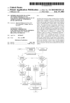
Likewise, there is a similar shortcut to enter angles in fields that
accept them. If you wanted to enter the angle, α, from the
illustration shown here, you would simply enter 1-2-3 in the
appropriate field. As soon as the cursor is moved from that field, the
angle formed by the three points entered will be entered in that field.
As with specifying a distance, you could also use the power button as
described above and tap the points of the angle in the correct order.
Another shortcut can be used to enter distances with fractional inches
(architectural units). Simply key in the feet, inches, and fractional
14
1
2
α
3
Getting Started
inches where each value is separated by a space and the fraction is
entered using a forward slash (/). For example, to enter 3 feet, 6 and
3/32 inches, you would key in 3 6 3/32. Once the cursor leaves that
field, the distance will automatically be converted to the appropriate
decimal distance.
If working with distances under 1 foot, it is acceptable to exclude the
feet value; for example "8 5/64" would be interpreted as 8 and 5/64
inches. Likewise, if entering a fractional distance under an inch, you
would only enter the fractional inch.
The following details should be considered when using the above
method to enter fractional inches:
1. When the job is configured for International Feet or US Survey
Feet, it is assumed that the distance entered is in the same units
as the job is configured for.
2. If the job is configured for meters, it is assumed that the
distances entered are in International Feet and will be converted
to meters when the cursor leaves the current field. (You cannot
use this method to enter a metric distance in fractional format.)
3. If a fractional inch is entered that cannot be evenly divided by
1/64 inch, it will automatically be converted to the nearest 64th
inch. This conversion would be negligible for survey data and
unlikely to occur.
An alternate method to using this shortcut is to tap the Quick Pick
button while the cursor is in a distance field that you want to change
and select AU Conversion. Enter the appropriate feet, inches and
fractional inches and tap Use . See the Reference manual for more
information on the AU Conversion screen.
15
User’s Manual
Point List Editor
Many screens contain a
button,
which accesses the Select Point(s) screen that
allows you to enter a simple list of points or a
list of points that describe a line that can
contain curves.
Examples of how to enter different lists of
points are displayed in the lower portion of the
screen. Once the list is entered, tap to
return to the previous screen.
Note: Spaces in point lists are ignored. They
are only used in the examples for clarity.
The examples for entering the three possible curve types are
explained in detail as follows:
•
7(8)9
The first example, defines a curve that passes through Points
7, 8 and 9, respectively.
•
7 ( 8, L ) 9
The second example defines a curve where Point 8 is the
radius point and the curve begins to the Left (from the point
of view of the radius point), turning from Point 7 to Point 9.
Note: When defining a curve with a radius point, the other two points
must be the same distance from the radius point for a solution.
•
16
7 ( 100, L, L ) 9
The third example describes a curve with a radius of 100,
using the same units as the job, that begins at Point 7,
turning to the Left (from the point of view of the radius point),
creating a Large arc (> 180°), and ending at Point 9.
Getting Started
Entering Distances in Other Units
When a distance is entered in a particular field, it is normally entered
using the same units that are configured for the current job, but
distances can also be entered that are expressed in other distance
units.
When entering a distance that is expressed in units that do not match
those configured for the job, you simply append the entered distance
with the abbreviation for the type of units entered. For example, if
the distance units for your current job were set to International Feet
and you wanted to enter a distance in meters, you would simply
append the distance value with an m or M for meters. As soon as the
cursor is moved to another field, the meters that were entered will be
converted to feet.
The abbreviations can be entered in lower case or upper case
characters. They can also be entered directly after the distance
value, or separated with a space. The following abbreviations can be
appended to an entered distance:
•
International Feet:
f or ft or ift
•
US Survey Feet:
usf or usft
•
Inches:
i or in
•
Meters:
m
•
Centimeters:
cm
•
Millimeters:
mm
•
Chains:
c or ch
17
User’s Manual
Quick Pick
The button is called the Quick Pick button.
This button is used to quickly access any of
several commonly-used routines. The list of
routines available from the Quick Pick button
can be customized and sorted in any order.
To access a screen with the Quick Pick button,
first tap and then tap the desired routine.
Customizing the Quick Pick List
If you want to customize the Quick Pick list,
tap and then scroll to the bottom of the list
and tap Edit Quick Pick. This opens the Quick
Pick Editor.
Tip: You can quickly get to the bottom of the
Quick Pick list by tapping then pressing the
up-arrow hardware button once.
The current Quick Pick list is displayed in the
right column and the routines that can be
added to the list are displayed in the left column, where the routines
that are already in the Quick Pick list are shown in bold.
To add a routine, first select the menu item from the Menu Item
dropdown list where that routine is normally accessed from the Main
Menu. (Not all routines can be added to the Quick Pick list. If a
routine is not listed, it cannot be added.)
Select the routine from the left column then tap the Add --> button
to add it to the Quick Pick list on the right.
18
Getting Started
The new routine will initially be placed at the bottom of the list. To
move it elsewhere in the list, select it and tap the Move Up or
Move Down buttons. (Any other routines in the Quick Pick list can
also be repositioned in this way.)
To remove a routine from the Quick Pick list, select it and tap the
<-- Remove button.
Tapping the Defaults button will revert the custom list back to the
default list. Since any changes will be lost, a prompt will first ask if
you are sure.
Smart Targets
Survey Pro has the ability to create and store custom configurations
for any number of prisms or other target types. These are called
Smart Targets.
Smart Targets are useful when working with multiple prisms on the
same job, particularly when the prisms have different characteristics
such as rod height and/or offset because the user can quickly switch
between different Smart Targets before taking a shot.
Smart Targets also provide a way to quickly switch between taking a
shot at a prism and taking a shot at a reflectorless target. The total
station EDM configuration is switched for you automatically.
Selecting Smart Targets
You can quickly select any existing Smart Target from a screen that
has an HR field. Tap the power button
corresponding with the
icon displayed next to the
HR field that you want to shoot. A
power button indicates a prism target type is currently selected. A
icon indicates a reflectorless target type is currently selected
All the available Smart Targets will be displayed in the upper
portion of the drop-down list. The Smart Targets listed will
depend on if you are selecting a Smart Target for your foresight
or your backsight.
Simply tap the Smart Target that you want to use from the drop19
User’s Manual
down list. The preset configuration for the selected Smart Target will
be automatically set.
Manage Smart Targets
Select Manage Smart Targets from the same drop-down list described
above to access the Manage Smart Targets screen. From here you
can create a new custom Smart Target or edit
any existing Smart Target.
Survey Pro includes two foresight Smart
Targets called My Prism and My Reflectorless,
respectively and one backsight Smart Target
called My Backsight Prism. These can be edited
or deleted, but at least one prism and one
reflectorless foresight Smart Target and at
least one prism backsight Smart Target must
exist at all times. Because of this, for example,
you would not be able to delete My Backsight
Prism unless another Smart Target with a
prism target type for your backsight was available. Similarly, you
would not be able to change My Reflectorless to a prism target type
unless you already had another foresight Smart Target configured
with a reflectorless target type.
To delete an existing Smart Target, tap it to select it and then tap
Delete .
Tapping Sort will sort the list of Smart Targets alphabetically.
You can also activate a Smart Target from this screen by tapping the
desired Smart Target to select it and then tapping Activate ,
although it’s faster to activate Smart Targets using the shortcut
described above. The active Smart Target is shown with a symbol
next to it.
20
Getting Started
To create a new Smart Target tap the Add…
button. To edit an existing target, tap it from
the list to select it and then tap Edit… . Either
option will open the Edit Smart Target screen.
The Smart Target Name you provide will be
shown in the drop-down list when you switch
between Smart Targets.
The Target Type field determines how the EDM
will be configured on the total station when
taking shots to the Smart Target. It can be
Prism when using a standard prism,
Reflectorless to perform distance measurements without a prism, Long
Range Prism, which increases the output power of the EDM for
shooting prisms at long distances, or On Gun, which uses the EDM
settings configured on the total station (Leica only). Not all target
types are supported by all total station.
Note: If using a Trimble S6/VX, there are special smart target
settings available, which are described under Smart Targets in the
Reference Manual.
The HR field will be the default rod height whenever this Smart
Target is selected. Updating the HR from any screen that has an
editable HR field while a Smart Target is selected will also save that
new value here, making it the new default HR for the current Smart
Target.
If the Add Offset to HR is checked, the offset entered in the
corresponding field will then be added to the rod height you provide.
(A negative value would subtract the offset from the HR.) This is
useful for people who use a device that always elevates their rod by a
fixed distance, but still want to use the rod height measurement
displayed on the rod for simplicity.
For example, if you were in the Backsight Setup screen and selected a
foresight Smart Target with a default HR of 5 feet and an HR offset
value of 1 foot, you would see 5.00 ift displayed in the foresight HR
field of the Backsight Setup screen, as well as every other editable
foresight HR field, but you would see 5.0+1.0 ift in every output-only
21
User’s Manual
HR field showing the HR entered plus the offset. (The raw data file
will also clearly note when a rod height offset is being applied.)
The Prism Constant field should contain the prism constant for the
prism associated with this Smart Target as long as a prism constant
is not also set in the total station. If a prism constant is set in Survey
Pro and on the total station, it will be applied twice resulting in
incorrect distance measurements for every shot.
If you are using a robotic total station that supports prisms that
output a target ID, the Use Target ID field will be available where you
can specify the target ID for the Smart Target.
If Use For Search is available and selected, the total station will only
look for the Target ID when it is searching for the target. Once the
target is found, it will track the prism, but it is possible for the total
station to start tracking a different reflector that comes into view. If
Use Always is selected, the total station will continuously monitor the
Target ID and only track the prism with the specified Target ID.
Tap
to close the Edit Smart Targets screen and save any changes.
Map View
from the command bar, or
from various screens
Many screens provide access to a map view. The map view is a
graphical representation of the objects in the current job.
Map View without basemaps
22
Map View with basemaps
Getting Started
There are different map views depending on from where the map
view is accessed and they can display slightly different information
such as a vertical profile.
The main map view is accessed from the Main Menu by tapping the
button at the bottom of the screen in the command bar. If you are
using basemaps, it is from this map view where the basemaps are
managed.
All other map views are accessed by tapping the
variety of screens.
button from a
A bar is shown at the bottom of every map view that indicates the
scale.
The buttons along the left edge of the screen allow you to change
what is displayed in the map view.
Tip: You can pan around your map by dragging your stylus across the
screen.
Zoom Extents Button: will change the scale of the screen so that
all the points in the current job will fit on the screen.
Zoom In Button: will zoom the current screen in by
approximately 25%.
Zoom Out Button: will zoom the current screen out by
approximately 25%.
Zoom Window Button: Allows you to drag a box across the
screen. When your finger or stylus leaves the screen, the map will
zoom to the box that was drawn.
Zoom To Point Button: Prompts you for a point name and then
the map view will be centered to the specified point with the point
label displayed in red.
Turn To Point Button: Tap this button and then tap a point in
the map view to automatically turn the total station to the selected
point. This is only available when a robotic total station is selected
and Remote Control is active in the Instrument Settings.
23
User’s Manual
Increase Vertical Scale: is only available when viewing a
vertical profile. Each time it is tapped, the vertical scale of the view
is increased.
Decrease Vertical Scale: is only available when viewing a
vertical profile. Each time it is tapped, the vertical scale of the view
is decreased.
Zoom Preview Button: will display only the points that are
currently in use (only available from certain map view screens).
Map Display Options: Accesses the Map Display Options screen,
described below.
Manage Basemaps: Accesses the Manage Basemaps screen,
described below (only available from the main map view, accessed
from the command bar button in Main Menu).
Basemaps
Basemaps can be used in jobs to more accurately display local objects
and terrain in the map view to give the surveyor a better idea of
where they are in relation to local land features.
There are two general types of basemaps – raster images and CAD
drawings. Raster images are usually created from photographs and
can accurately display the local terrain with great detail. CAD
drawings are created from CAD software and will typically display
points, roads, boundaries and any other objects that can be drawn
with lines.
Basemap Files
Survey Pro supports basemap files from AutoCAD, GeoTiff, and TDS.
Since basemap files can be large in size, the following points should
be considered when managing basemap files:
24
Getting Started
•
Before you can use a basemap in
Survey Pro, you need to copy the
appropriate basemap files from a PC to
the same directory where your current
job is located. If the basemap files are
stored in a different directory and then
added to the current job, the files will
be copied to the job’s directory.
•
If you use the Save As routine and save
the current job to a new directory, any
basemaps associated with that job will
be copied to the new location.
Manage Basemaps
Once the basemap files are stored on the data collector, they must be
added to the current job before they can be viewed in the map view.
1. To add basemaps, open the Main Map View by tapping the
button in the command bar from the Main Menu.
2. From the main Map View, tap the
button to open the Manage Basemaps
screen shown here.
3. Tap the Add… button. This will open a
new screen where you can select the
basemap that you want to add to the
current job.
4. Once a basemap is added, it will appear in
the list in the Manage Basemaps screen.
5. Repeat Steps 3 and 4 to add any additional
basemaps.
25
User’s Manual
Basemaps are drawn to the screen in the
reverse order that they are listed in the
Manage Basemaps screen, where the first
basemap in the list is the last one drawn,
and thus, will be drawn "on top" of any
other basemaps. This is important to
remember if any basemaps overlap since if
a raster basemap were drawn on top of
another basemap, it would cover any
basemaps below it.
The list shown contains a vector basemap,
tds.dxf that occupies the same area as the
other two basemaps, which are raster
basemaps. The vector basemap is at the
top of the list so the points and lines it
contains will be drawn last and appear on
top of the two raster basemaps.
Raster basemap drawn first.
6. To change the order of the basemaps in
the list, select a basemap and tap the
Move Up or Move Down buttons to
move it up or down in the list,
respectively.
7. To remove any basemap from the list,
select it and tap Remove . This will
remove the basemap from the list and
un-associate it from the current job.
(This will not delete the corresponding
basemap file.)
Vector basemap drawn last.
Resulting map view with both basemaps in
view.
26
Getting Started
8. The colors of the objects in vector basemaps
can be modified by selecting the basemap
and then tapping Edit… to open the Edit
Basemap screen.
The Settings Screen
The Settings screen is used to control all of the settings available for
your total station, data collector, current job, and Survey Pro
software.
Most of the settings remain unchanged unless you deliberately
change them, meaning the default settings are whatever they were
set to last. For example, if you create a new job where you change the
direction units from azimuths to bearings and then create another
new job, the default direction units for the new job will be bearings.
Survey Pro behaves in this way since most people use the same
settings for a majority of their jobs. This way, once the settings are
set, they become the default settings for all new jobs and current jobs.
Some settings are considered critical and are therefore stored within
the job. The following settings are stored within a job and will
override the corresponding settings in the Settings screen when it is
opened:
•
Scale Factor – Surveying Settings Card
•
Earth Curvature On or Off – Surveying Settings Card
•
Units for Survey Data (distances) – Units Settings Card
•
North or South Azimuth – Units Settings Card
•
Angle Units – Units Settings Card
27
User’s Manual
•
GPS setup information such as localization, mapping plane,
etc. (Requires GPS Module)
The Settings screen actually consists of several
independent screens where each individual
screen contains different types of settings.
There are two ways to navigate to the various
screens. The first method is to tap the
button to drop down the list of available
screens and then tap on the desired screen
from the list to open it. The second method is
to tap the buttons to the side of the screen title,
which will open the previous or next screen
respectively. For example in the screen shown,
to open the previous
you could tap
(General Settings) screen, or tap
to open the next (Units
Settings) screen. Repeatedly tapping either of these buttons will
cycle through all the available screens.
Consult the Reference Manual for an explanation of each field on
every Settings screen.
If using a Bluetooth total station, refer to the Bluetooth section on
Page 294.
File Management and
ForeSight DXM
Survey Pro uses a variety of files to store data and information
about your project. The files include the main data file, the .JOB file,
and the raw data file, the .RAW file, and several other supplementary
files that Survey Pro can use for additional information. To help
manage this data and to supplement Survey Pro capabilities, TDS
has an office product called ForeSight DXM.
ForeSight DXM is a complete data management tool that works
directly with Survey Pro data files. ForeSight DXM can make any
project easier to manage and makes doing every day tasks, such as
downloading, quick and easy. ForeSight DXM has a variety of
28
Getting Started
analysis tools, geodetic tools including projection setups, and the
capability to convert TDS data files into many other formats,
including LandXML, for use in CAD.
ForeSight DXM makes the field-to-office and the office-to-field
process seamless and easy. If you don’t already own a copy of
ForeSight DXM, contact your TDS Dealer for more information. You
can also download a full-featured demonstration copy of ForeSight
DXM from the TDS Web site at www.tdsway.com.
Job Files
Every job that is used with TDS Survey Pro actually consists of at
least two separate files; a job file and a raw data file. Each file
performs a different role within the software.
A job file can be created in the Data collector, or on a PC using TDS
ForeSight DXM (or other PC software) and then transferred to the
Data collector. It is a binary file that has a file name that is the same
as the job name, followed by a *.JOB extension. A job file is similar to
the older TDS-format coordinate file, except in addition to storing
point names and their associated coordinates, a job file also contains
all of the line work as well.
When you specify points to use for any reason within Survey Pro, the
software will read the coordinates for the specified points from the job
file. Whenever you store a new point within Survey Pro, the point is
added to this file.
A job file can be edited on the Survey Pro when using the Edit Points
screen. Since a job file is binary, it requires special software for
editing on a PC, such as TDS Survey Link. It can also be converted to
or from an ASCII file using Survey Link. (Refer to the Survey Link
documentation for this procedure.)
When a job file is converted to an ASCII file, the resulting file is
simply a list of points and coordinates. Each line consists of a point
name, northing or latitude, easting or longitude, elevation or elliptical
height, and a note where each value is separated by a comma.
29
User’s Manual
Raw Data Files
A raw data file is an ASCII text file that is automatically generated
whenever a new job is created on Survey Pro and cannot be created
using any other method. It has the same file name as the current job
file (the job name), followed by the *.RAW extension.
A raw data file is essentially a log of everything that occurred in the
field. All activity that can create or modify a point is written to a raw
data file. Survey Pro never "reads" from the raw data file – it only
writes to the file. Since a raw data file stores all of the activity that
takes place in the field, it can be used to regenerate the original job
file if the job file was somehow lost. This process requires the TDS
Survey Link software.
Since a raw data file is considered a legal document, it cannot be
edited using any TDS software other than appending a note to it
using the View Raw Data screen. Editing a raw data file would
invalidate all of its contents and is not supported in any way by TDS.
When viewing a raw data file on a PC using a simple text editor or on
Survey Pro using the View Raw Data screen, the file is shown
unaltered, which can appear somewhat cryptic. When viewing the file
from within Survey Link, the codes are automatically translated on
the screen to a format that is easier to understand.
30
Getting Started
Control Files
The current job can be configured to access the points from another
job stored on the data collector. When the current job is using points
from another job, that other job is called a Control File and the points
in the control file are called Control Points. (Any non-point objects in
a control file are always ignored.)
A control file can be selected from the New Job wizard when creating
a new job, or the File Import Control screen can be used to select a
control file for an existing job, or to manage the current control file.
See the Reference Manual for more information on these screens.
There are two methods for accessing control points: imported control
points and external control points. Each method has advantages and
disadvantages, which are explained below.
Import Control File
When a control file is imported, the control points are copied into the
current job and stored on a special layer called CONTROL.
Importing control points provides improved RAW data consistency
since each control point is written to the raw data file as a store point.
This can significantly help when regenerating points from RAW data
and generating reports in the office.
Importing control points may not be the best method when using very
large control files, while collecting relatively small sets of points since
the imported control points can make the current job very large with
too many points to easily manage.
Importing control points is also not recommended when you want to
switch between different control files from the current job.
31
User’s Manual
External Control File
When using an external control file, the points in the control file are
simply linked to the current job and do not become a permanent part
of the current job. Because of this, an external control file can later
be unlinked, or cleared from the current job.
Some users prefer to keep a set of known points in a separate control
file when repeatedly working on new jobs in the same general area.
That way when they return to the job site, they can create a new job,
but select the external control file to easily have access to the known
control points.
Once an external control file is selected, the control points can be
used in the same way as the job’s points with the following
exceptions:
32
•
An external control file has read only attributes. This means
that the points in the control file cannot be modified or
deleted; they can only be read. For example, you can select a
control point to use as an occupy point during data collection
or as a design point during stake out, but you could not use a
control point for a foresight where you intend to overwrite the
existing coordinates with new coordinates. You would also be
unable to modify a control point from the Edit Points screen.
•
Since the points in an external control file are shared with the
points in the current job, you cannot open an external control
file if any of the point names used in it are also used in the
current job. If you attempt to do so, a dialog will tell you that
a duplicate point name was encountered and the control file
will not be opened.
Getting Started
Description Files
A Description File is used to automate the task of entering
descriptions for points that are stored in a job. They are especially
useful when the same descriptions are frequently used in the same
job.
A description file is a text file containing a list of the descriptions that
you will want to use with a particular job. The file itself is usually
created on a PC, using any ASCII text editor such as Notepad, which
is included with Microsoft Windows. It is then saved using any file
name and the .txt extension and then transferred to the Data
Collector.
It is important to realize that when you use a more sophisticated
application, such as a word processor to create a description file, you
must be careful how the file is saved. By default, a word processor
will store additional non-ASCII data in a file making it incompatible
as a description file. However this can be avoided if you use the File >
Save As… routine from your word processor and choose a Text Only
format as the type of document to save. For more information on
creating a text file using a word processor, refer to your word
processor’s documentation.
Description files can be created in two different formats; one includes
codes and the other does not. The chosen format determines how
descriptions are entered. Each format is described below.
Description Files without Codes
A description file that does not contain codes is
simply a list of the descriptions that you will want to
use in a job. The content of a sample description file,
without codes, is shown here.
The following rules apply to description files without
codes:
•
Each line in the file contains a separate description.
•
A description can be up to 16 characters in length (including
spaces).
33
User’s Manual
•
A description can contain any characters included on a
keyboard.
•
Descriptions do not need to be arranged in alphabetical order.
(Survey Pro does that for you.)
•
Descriptions are not case sensitive.
To use a description from a description file,
simply start typing that description in any
Description field. (You can experiment with
descriptions in the .Survey ,
Traverse / Sideshot screen.) Once you start
typing a description, a dropdown list will
appear displaying all of the descriptions in the
descriptor file along with all the descriptors
that have been used in the current job in
alphabetical order. If the first letter(s) that
you typed match the first letters of a
description in the descriptor file, that
description will automatically be selected in the dropdown list. Once
it is selected, you can have that description replace what you have
typed by pressing [Enter] on the keypad. You can also use the arrow
keys to scroll through the dropdown list to make an alternate
selection.
Description Files with Codes
A description file that uses codes is similar to those
without codes, except a code precedes each description
in the file. A sample description file with codes is
shown here.
The following rules apply to description files that use
codes:
34
•
Each line in a description file begins with a code, followed by
a single space, and then the description.
•
A description code can consist of up to seven characters with
no spaces.
Getting Started
•
Description codes are case sensitive.
•
The description is limited to 16 characters.
•
Descriptions can include any character included on a
keyboard.
To use a description from a description file with codes simply type the
code associated with the desired description in any Description field.
As soon as soon as the cursor moves out of the Description field, the
code is replaced with the corresponding description. For example, if
you typed PC in a description field while using the description file
shown above, PC would be replaced with PROPERTY CORNER once
the cursor was moved to another field.
You can combine a description with any other text, or combine two
descriptions by using an ampersand (&). For example, entering
NB&PC would result in a description of NEW BACKSIGHT
PROPERTY CORNER. This method also works when spaces are
included with an ampersand. For example, entering NB&PC would
have the same result as entering NB & PC.
Opening a Description File
Once a description file is created and stored in the data collector, it is
activated with the following steps:
1. Select .Job , Settings from the Main Menu.
2. Select the Files tab and tap the Browse button in the Description
File section of the screen.
3. All of the files with a .txt extension will be displayed. Select the
file that you want to use and tap Open .
4. If the description file contains codes, check the This File Uses
Codes checkbox.
35
User’s Manual
Feature Codes
As explained above, a description or descriptor codes can be used to
help describe a point prior to storing it, but this can be a limited
solution for describing certain points.
Survey Pro also allows you to describe any object using feature codes.
Feature codes can be used to describe objects quickly and in more
detail than a standard text description, particularly when data is
collected for several points that fit into the same category. For
example, if the locations for all the utility poles in an area were being
collected, a single feature code could be used to separately describe
the condition of each utility pole.
When describing an object using feature codes, a selection is made
from any number of main categories called features. Once a
particular feature is selected, any number of descriptions can be
made from sub-categories to the selected feature called attributes.
In general, a feature describes what an object is and attributes are
used to describe the details of that object.
To take advantage of feature codes, a feature file must first be created
using the TDS Survey Attribute Manager, which is included in
Version 7.2, or later of the TDS Survey Link software.
The TDS Survey Attribute Manager can also be used to view or
modify the selected features in a particular job and to export them to
any of several different file formats for use in other popular software
packages.
Note: You can switch between different feature code files in mid-job,
but if a collected attribute does not match an attribute in the current
feature code file, it can still be viewed, but not edited.
For more information on creating a feature file, refer to the Survey
Attribute Manager section of the Survey Link manual.
36
Getting Started
Features
The primary part of a feature code is called a feature. Features
generally describe what an object is. Two types of features are used
in Survey Pro: points and lines, which are described below.
When assigning a feature to data that was collected in Survey Pro,
only features of the same type are available for selection. For
example, if selecting a feature to describe a point in a job, only the
point features are displayed. Likewise, if selecting a feature to
describe a polyline, only the line features in the feature file are
displayed.
•
Point Features
A point feature consists of a single independent point.
Examples of a point feature would be objects such as a tree, a
utility pedestal, or a fire hydrant.
•
Line Features
A line feature consists of two or more points that define a linear object,
such as a fence or a waterline. In Survey Pro, these are stored as
polylines, but line features can also be used to describe alignments.
Attributes
A feature, by itself, would not be useful in describing a point or line
with much detail since a feature only helps describe what the stored
point is. Attributes are used to help describe the details of the object.
Attributes are either typed in from the keyboard or selected from a
pull-down menu and fall into the following three categories.
•
String Attributes
A string attribute consists of a title and a field where the user can type
any characters from the data collector’s keypad up to a specified
maximum length. An example of a string attribute is an attribute titled
Notes where the user would type anything to describe a feature.
•
Value Attributes
A value attribute accepts only numbers from the keypad. These
attributes are setup to accept numbers that fall in a specified range.
Some examples of a numeric attribute would be the height of a tree or a
utility pole’s ID number.
37
User’s Manual
•
Menu Attributes
A menu attribute is an attribute that is selected from a pull-down menu
rather than typed in from the keypad. Menu items can also have submenu items. For example, you could have a feature labeled Utility with
a pull-down menu labeled Type containing Pole and Pedestal. There
could also be sub-menu items available that could be used to describe
the pole or pedestal in more detail. Menus can only be two levels deep,
but there is no limit to the number of items that can be listed in a pulldown menu.
Using Feature Codes in Survey Pro
Before you can use features and attributes to describe points in
Survey Pro, you must select a valid feature file to use with the
current job.
To select a feature file, open the Job , Settings
screen and then select Files Settings. Tap the
bottom Browse… button then locate and select
the appropriate *.FEA feature file.
Once a feature file is selected for the current
job, you can configure Survey Pro to prompt for
attributes whenever a point, line, or alignment
is stored. There are three screens within the
Job Settings screen to configure this prompt.
There is a ; Prompt for Attributes checkbox in
the Surveying Settings, the Stakeout Settings
and the General Settings. The first affects if you are prompted for
attributes only when an object is stored from the routines within the
Survey menu. Likewise, the second affects only objects stored from
the routines in the Stakeout menu. The prompt in the General
Settings affects if you are prompted for attributes when an object is
stored from any other routines, such as the COGO routines.
The features and attributes for existing points, polylines, and
alignments can also be edited using the Edit Points and Edit
Polylines and Edit Alignments screens, respectively.
38
Getting Started
Layers
Survey Pro uses layers to help manage the data in a job. Any number
of layers can exist in a job and any new objects can be assigned to any
particular layer. For example, a common set of points can be stored
on one layer and another set can be stored on a different layer.
The visibility of any layer can be toggled on and off, which gives full
control over the data that is displayed in a map view. This is useful
to reduce clutter in a job that contains several objects. The objects
that are stored on a layer include points, polylines, and alignments.
TDS ForeSight can read a JOB file and output an AutoCAD DXF file
containing all the original layer information. This conversion can
also be performed using TDS Survey Link 7.2, or later via the Survey
Attribute Manager, which is included as part of that program.
Layer 0
Layers can be added, deleted and renamed with the exception of
Layer 0. Layer 0 is a special layer that must exist in every job. It
cannot be deleted or renamed.
Layer 0 provides two main functions: compatibility with AutoCAD;
and is used as a layer for the storage of objects that are not assigned
to any other layer. Since all the objects in a job have to be assigned to
a layer, Layer 0 is always there so a situation cannot occur where an
object is stored, but does not exist on any layer.
Other Special Layers
Some layers are automatically created, but unlike Layer 0, these
layers behave exactly the same as any user-created layer; they can be
renamed or deleted. Whenever a control file is selected for a job, a
Control layer is automatically created and the points in the control file
are stored to that layer. (Any non-point objects in a control file are
always ignored.)
39
User’s Manual
Similarly, whenever a new job is created, a Points layer is
automatically created and selected as the active layer. The active
layer is the default layer where any new objects will be stored.
Managing Layers
You can configure Survey Pro to prompt for a layer whenever an
object is stored. If this prompt is turned off, any new objects that are
stored will simply be stored to the active layer. There are three
screens within the Job Settings screen to configure this prompt.
There is a ; Prompt for Layer checkbox in the Surveying Settings, the
Stakeout Settings and the General Settings. The first affects if you
are prompted for a layer only when new data is stored from the
routines within the Survey menu. Likewise, the second affects only
data stored from the routines in the Stakeout menu. The prompt in
the General Settings affects if you are prompted for a layer when data
is stored from any other routines, such as the COGO routines.
Most layer management is performed from the
Job Manage Layers screen. This screen
allows you to add, delete, rename and change
the visibility of the various layers. You can also
set the active layer from here. This screen is
also available from several different locations,
such as the new Map Display Options screen
and any of the controls that allow you to select
layers.
Changing the Active Layer
To change the active layer, tap the desired layer and then tap the
Set Active button. There must always be an active layer and there
can only be one active layer at a time. The active layer is marked
with the symbol.
Creating a New Layer
A new layer can be created by tapping New… , which opens the New
Layer dialog box where a name and if the new layer should be visible
is entered.
40
Getting Started
Changing a Layer Name or Visibility
Selecting a layer and then tapping Edit… opens the Edit Layer
dialog box where the name and visibility can be changed for the
selected layer. You can also edit a layer by double-tapping on it.
(Layer 0 cannot be renamed.)
Deleting a Layer
You can only delete an empty layer. If a layer contains any objects,
they must first be moved to a different layer. To delete a layer, select
the layer and tap Delete . (Layer 0 cannot be deleted.)
Moving Objects from One Layer to Another
The objects on a layer can be moved to a different layer using the
object’s appropriate edit screen. For example, to move several points
from one layer to another, select the desired points in the Edit Points
screen and tap Edit . Select the layer you want to move them to and
tap .
41
User’s Manual
Working with 2D Points
Most people work with 3D points, but Survey Pro also allows you to
work with 2D points (points without elevations). You can also work
with a combination of both 3D and 2D points.
It is important to remember that data collected from a 2D point will
also be 2D, so care should be taken when working without elevations.
To assist the user, various warnings will appear when working with
2D points.
Some routines require elevations and are therefore inaccessible when
working with 2D points. When attempting to perform a routine using
a 2D point that requires 3D points, the following error will result:
"This operation requires an occupy point with a valid
elevation."
Examples of routines that require elevations and do not support 2D
points include:
•
Slope Staking
•
Stake DTM
•
Vertical Angle Offset
•
All Road Layout Routines
You can quickly see if any 2D points exist in the current job by
opening the .Job , Edit Points screen and scrolling down the Elevation
field. Any point where the elevation is shown as ‘---’ is a 2D point.
You can convert a 3D point to a 2D point by simply editing the point
and deleting the elevation.
The items below explain what to expect when working with 2D points
in a variety of situations.
Traverse / Side shot
Setting up over a 2D occupy point will result in any traverse or side
shot taken from that point to also have no elevations. When a 2D
point is selected as the occupy point in the Backsight Setup screen,
the following message will be displayed:
42
Getting Started
"Note: Selected occupy point has no elevation. All points
computed with this point will have no elevation
computed for them."
An elevation adjustment on a traverse containing any 2D points is
not possible. If an attempt is made to do so, the following message is
displayed:
"Traverse contains a 2D point. Cannot adjust
elevations."
Point Stake
When performing point stake using a 2D point, no cut/fill information
is provided. This is the case when either the occupy point or the
stake point is 2D. Cut/fill information is only provided when both the
occupy point and stake point have elevations.
Offset Stake
Offset stakeout functions similar to point stake, although cut/fill
information can be generated when using a 2D alignment and 3D
occupy point when a design elevation for the stake point is provided.
The following message is displayed in this situation:
"A 2D alignment has been selected; no cut/fill
information will be computed unless a design elevation
is entered."
Slope Stake
Slope staking is not possible when using 2D points since elevations
are required.
Control Points
Control points can be all 2D, all 3D, or a mixture of both. The same
limitations for working with 2D non-control points will apply when
working with 2D control points.
43
User’s Manual
Polylines
Lines can be added to your project that can represent anything such
as a roadway, a building, or a lot boundary. These lines are referred
to as polylines. Polylines can be compared to the point lists used in
other TDS data collection software. They can consist of several
individual curved and straight sections. A point must be stored in the
project for all the locations on the polyline where a new section begins
and ends.
Polylines can be used to compute information such as the perimeter
and area for a lot boundary. They can also make it easier to compute
and store offset points for the sides of a roadway when a polyline
exists that defines a roadway centerline.
Refer to the Reference Manual for information on all the screens that
are used to create and edit polylines.
Alignments
Alignments are similar to polylines in that they define specific lines
in the current job and typically describe the centerline of a road. An
alignment can then be used in the Offset Staking, Offset Points,
Offset Lines, and Slope Staking screens. Unlike polylines,
alignments do not need points for the locations where the alignment
changes (called nodes).
Alignments are created by separately defining the horizontal and
vertical details of a line. Although no points are required to define an
alignment, the starting position must be tied to a specific location in
the current job, the POB, which can be defined by an existing point or
known coordinates.
The horizontal and vertical details of an alignment are defined in
sections. The first horizontal and vertical section always begins at
the specified starting location and each new segment is appended to
the previous horizontal or vertical segment.
44
Getting Started
Once all the horizontal and vertical alignment segments are defined,
Survey Pro merges the information to create a single 3-dimensional
line.
The vertical alignment (VAL) must be equal in length or greater than
the horizontal alignment. The HAL must not be greater than the
VAL.
Creating an Alignment
In this step-by-step example, we will create an alignment that has all
the possible horizontal and vertical segment types.
1. Select .Job , Edit Alignments from the
Main Menu. If any alignments exist in the
current job, they will be listed in this
screen. An existing alignment can then be
edited or deleted, but for this example, we
will create a new alignment.
2. Tap New… to create a new alignment.
This will open the Edit Alignments screen
where you can begin adding horizontal and
vertical segments.
3. Tap the POB tab and enter North, East and
Elev coordinates of 5000, 5000, 100. This
will be the starting location of the
horizontal and vertical definition.
(Alternatively, you could define the starting
location by tapping the Location /
Point button where Point is displayed
and then select an existing point.)
45
User’s Manual
Horizontal Alignment
4. Tap the HAL (Horizontal Alignment) tab
and then tap the Insert button. This will
open the Insert Segment screen where the
first horizontal alignment segment can be
defined.
5. Tap the Line tab to insert a straight line
segment. Enter a Length of 100 and an
Azimuth of 0.
6. Tap to add the segment to the horizontal
alignment. You will return to the Edit
Alignment screen where the new segment
is displayed. The graphic shows every
horizontal segment entered so far with the
selected segment in bold. The dot in the
picture indicates the beginning of the
selected segment (in this case it is the end).
This is where the next segment will be
placed when using the Insert button.
7. Tap the Insert button again and then tap
the Arc tab to insert a horizontal curve.
8. Enter a Radius of 100, a Delta of 45
and select a Right turn. Check the Make
this segment tangent to previous checkbox so
that the curve will be positioned so the
entrance to the curve is tangent to the end
of the previous segment.
9. Tap to add the segment to the horizontal
alignment.
46
Getting Started
Note: A new segment can be inserted between two existing segments
by selecting the existing segment that is to occur after the new
segment and then tapping the Insert button.
10. With End selected, tap the Insert button
again and then tap the Spiral tab to insert a
spiral curve.
11. Enter a Radius of 100, a Length of 200,
select a Right of turn and a CS to ST
direction, and check the Make this segment
tangent to previous checkbox.
12. Tap to add the segment to the horizontal
alignment.
Note: When creating a new horizontal segment
and using the Make this segment tangent to
previous option, the new segment will appear in
the Edit Alignment screen tagged with a (P)
(see picture). This means that if the previous
horizontal segment is edited or deleted, thus
changing the orientation, all subsequent
horizontal segments that have the (P) tag will
also be adjusted so they will remain tangent to
the previous segments.
This does not hold true for vertical alignment segments. Vertical
segments do not have the Make this segment tangent to previous option
and will always begin with the specified starting grade unless they
are manually modified.
47
User’s Manual
Vertical Alignment
We have now added all available horizontal segment types. Next, we
will define the vertical alignment.
Since the horizontal and vertical alignments are defined
independently of each other, the first vertical segment that is defined
will start at the same POB defined above in Step 3.
13. Tap the VAL (Vertical Alignment) tab and
then tap the Insert button.
14. Tap the V. Grade tab to insert a grade.
Enter a Length of 150 and a Grade of 4%.
15. Tap to add the segment to the vertical
alignment.
16. With End selected, tap the Insert button
again and then tap the V. Curve tab to
insert a parabolic vertical curve. Enter a
Length of 250 and tap the Get Previous
Grade button to automatically set the Start
Grade to the ending grade of the previous
section. Enter an End Grade of -2%.
17. Tap to add the segment to the vertical
alignment.
48
Getting Started
18. Tap the General tab and enter a Description
of Roadway.
19. Tap from the Edit Alignment screen to
return to the Add/Edit Alignments screen
where the new alignment is stored and
displayed.
You have now created a new alignment using
all the available types of segments. You can
select the new alignment for use in the Offset
Staking, Offset Points and Offset Lines
routines.
Note: If the horizontal and vertical alignments end at different
stations, they can only be processed in the staking routines as far as
the end of the shortest alignment.
49
Conventional Fieldwork
This section will explain how to get started using Survey Pro to
collect data from a total station and perform stake out. It is assumed
that you are familiar with the operation of your total station. (GPS
surveying begins on Page 187.)
The first section describes the backsight setup procedures for various
scenarios. The next section walks you through the steps involved to
setup and perform a simple side shot and traverse shot. The third
section walks you through a simple point-staking example.
The remainder of the chapter illustrates the procedures to perform
the more complex routines in the Survey Pro software in a step-bystep manner. They are intended to explain only how to use a
particular routine without the need for you to enter any specific
values to read through the example.
When beginning any job, the setup is the same; you need to establish
an occupy point and a backsight.
The occupy point is the point where you will setup the total station.
The coordinates for the occupy point must exist in the current job or
active control file. They can be assumed coordinates; known
coordinates; or computed with the resection routine. (Control files
and the resection routine are discussed later.) Any point in the
current job can be an occupy point.
Once an occupy point is established, the second reference you need is
a backsight point or direction. This can be in the form of a point
stored in the current job, or an azimuth or bearing.
The horizontal angles recorded during data collection are relative to
the backsight. If a point is not available in the job to use as a
backsight, you can assume a backsight direction or you can use the
solar observation routine, described later, to establish a backsight.
The scenarios below will describe four different possibilities for
defining a backsight.
51
User’s Manual – Conventional Mode
Scenario One
You know the coordinates and locations for two points on your lot and
want to occupy one and use the other as a backsight.
Solution
1. Create a job using the coordinates for one of the known points as
the first point.
2. Use the Edit Points routine to add a second point using the
coordinates for the remaining known point.
3. From the Backsight Setup screen, set the Occupy Point field to the
point number of one known point and setup the total station over
that point.
4. Toggle the .BS Direction. / .BS Point. button to BS Point. and
enter the point name for the second known point in that field.
20. Aim the total station toward the other point, zero the horizontal
angle on the instrument, and tap Solve , then (close). If the
Always Prompt for Backsight Check option is checked in the Job >
Settings > General screen, you will be prompted to check your
backsight.
You are now ready to start your survey.
Scenario Two
You have found two points on your lot and know the azimuth between
them, but you do not have coordinates for either.
Solution
1. Create a job using the default coordinates for the first point.
2. From the Backsight Setup screen, set the Occupy Point field to the
point that was just created.
3. Setup the total station over the point where the known azimuth is
referenced.
4. Toggle the .BS Direction. / .BS Point. button to BS Direction. and
enter the known azimuth to the second point here.
52
Conventional Fieldwork
5. Aim the total station toward the second point, zero the horizontal
angle on the instrument, and tap Solve , then (close).
You are now ready to start your survey.
You may want to take a side shot from the Traverse Sideshot screen
to the backsight point so that you have coordinates for it. The
horizontal angle would remain at zero during this shot.
If you later find true State Plane coordinates for any of the points in
your job, you can use the Translate routine to adjust all the
coordinates accordingly.
Scenario Three
You have one point established on your lot and you know the azimuth
to an observable reference.
Solution
1. Create a job using the coordinates of the established point for the
first point. If the coordinates are unknown, accept the default
coordinates.
2. From the Backsight Setup screen, set the Occupy Point field to the
point that was just created.
3. Setup the total station over the established point.
4. Toggle the .BS Direction. / .BS Point. button to BS Direction. and
enter the azimuth to the observable reference here.
5. Aim the total station toward the observable reference, zero the
horizontal angle on the instrument, and tap Solve , then
(close). If the Always Prompt for Backsight Check option is checked
in the Job > Settings > General screen, you will be prompted to
check your backsight.
If you later find true State Plane coordinates for any of the points in
your job, you can use the Translate routine to adjust all the
coordinates accordingly.
53
User’s Manual – Conventional Mode
Scenario Four
You have only one known point on a job.
Solution
You have two options in this situation. One, you can assume an
azimuth for an arbitrary backsight reference and rotate the job later
using the Rotate routine once you have determined the actual
orientation.
Secondly, you can use the Sun Shot routine to determine an azimuth
to an arbitrary reference.
Summary
In general, you would follow these steps when you begin working on a
job.
1. Create a new job or open an existing job.
2. Setup over the Occupy Point.
3. Aim the total station toward the backsight and zero the
horizontal angle on the instrument.
4. Fill in the Backsight Setup screen and tap Solve , then (close).
If the Always Prompt for Backsight Check option is checked in the
Job > Settings > General screen, you will be prompted to check
your backsight.
5. Start your survey.
Note: You should enter the correct Height of Instrument and Height of
Backsight distances in the Backsight Setup screen if you plan to check
your backsight using the Check by Distance routine.
54
Conventional Fieldwork
Note: If the Backsight Circle displays a non-zero value, the angle
displayed is subtracted from all horizontal angles that are read
during data collection and the resulting points are adjusted
accordingly. This will happen after survey with true azimuths or
performing stakeout in a special mode. If you do not want this to
happen, you should change this value to zero from the Backsight
Circle dialog box by tapping the Backsight Circle button.
Most non-staking related data collection is performed from the
Traverse / Sideshot screen. When you take a shot using the Traverse
button, the routine expects that you will eventually be occupying the
foresight that you are shooting and backsighting your current occupy
point. When you are ready to setup on the next point, the occupy,
foresight and backsight points will automatically be updated
accordingly.
After taking a shot using the Side Shot button, the routine does not
expect the total station to be moved before the next shot and will
therefore only automatically advance the foresight point.
55
User’s Manual – Conventional Mode
Data Collection Example
This section illustrates the necessary setup and usage of the Traverse
/ Side Shot screen, which is the primary screen used during data
collection. We will create a new job and manually add another point
to the job to use as a backsight. We will run in manual mode so the
shot data must be entered manually. This example and the following
stakeout example are the only examples that are designed where the
user should follow along and enter the values in their data collector
as they are provided in the example.
Setup
1. Create a new job.
a. From the Main Menu, select File ,
Open / New .
b. Tap New… to open the Create a New
Job screen
c.
56
Enter any job name that you wish in
the Job Name field and tap Next > .
Conventional Fieldwork
d. For this example, simply accept the
default job settings and tap Next > .
Note: When creating a new job, it is important
that the Units for Distances field be set to the
correct units. This allows you to seamlessly
switch between different units in mid-job.
Problems can arise if these units are
inadvertently set to the incorrect units prior to
entering new data. For example, assume you
created a control file by hand-entering a list of coordinates in a new
job where the job was set to International Feet and the coordinates
were in US Survey Feet. Now assume you created another new job
and correctly set it to US Survey Feet. If you then selected the
previous job as a control file for the new job, the display of all of the
coordinates in the control file would be converted from Feet to US
Survey Feet.
e.
Accept the default coordinates for the
first job point by tapping Finish .
57
User’s Manual – Conventional Mode
2. Check the Job Settings.
a. Tap Job , Settings from the Main
Menu to open the Settings screen.
b. Select the Instrument card if it is not
already selected and make sure the
Manual Mode profile is activated. If the
symbol is not shown next to it, select
Manual Mode and tap Activate .
c.
For this example, select the Surveying
Settings card and un-check all the
checkboxes.
d. Tap
to save the job settings.
3. Add a backsight point to the job.
a. Select Job , Edit Points from the Main
Menu.
58
Conventional Fieldwork
b. Tap Insert… and enter a new point using the General and
Location cards with the following values, as shown: Point
Name: 2
Northing: 5050
Easting: 5050
Elevation: 100
Description: Backsight
and then tap .
4. Set up your backsight. In this example, we
will set up on Point 1 and backsight Point
2, which was just created.
a. Access the Survey , Backsight Setup
screen.
b. In the Occupy Point field, enter 1 as the
point name.
Tip: You can also select an existing point from a map view or
from a list by using the
power button.
59
User’s Manual – Conventional Mode
c.
Enter an HI and HR of 5 feet each.
d. Toggle the .BS Direction. / .BS Point. button to BS Point. and
enter 2 as the point name.
e.
Leave the Fixed HR at Backsight field unchecked.
f.
Tap Solve… to open the Backsight
Solved screen.
g. Confirm that the BS Circle value is zero.
If not, change it to zero.
h. Tap the Send Circle button. This
would normally zero the horizontal
angle on the instrument and is a
required step to properly exit from the
screen.
60
i.
Tap to exit from the Backsight
Solved screen. The map view will open
showing your current setup.
j.
Tap
(close) to continue.
Conventional Fieldwork
Performing a Side Shot
5. Access the Survey , Traverse / Sideshot screen and fill in the
appropriate fields. The backsight
information is displayed at the top of the
screen. At this point, it is assumed that
your total station is over the occupy point
and its horizontal angle was zeroed while
aiming toward the backsight.
a. In the Traverse / Sideshot screen, enter
the following data if not already
entered:
Foresight: 3
Description: SS
HR: 5
These values will define the point name, description, and rod
height for the next point that is stored.
b. Assuming that the total station is aiming toward the prism,
which is located over the foresight, tap Side Shot . This would
trigger the total station to take a shot, compute coordinates
for the new point and store it. Since we are running in
manual mode, we will enter the shot data from the keypad.
c.
Enter the following data:
Angle Right: 70
Zenith: 90
Slope Dist: 100
and then tap . The new point is
computed and stored. The Foresight
point will automatically advance to the
next available point name and the
information from the last shot is
displayed on the screen.
61
User’s Manual – Conventional Mode
d. You can see a graphical representation
of the previous shot by tapping the Map
tab. See Page 22 for more information
on the Map View.
Performing a Traverse Shot
6. The steps involved in performing a traverse shot are nearly
identical to performing a side shot. The difference is you must
specify if you plan to move the total station to the current
foresight point after the shot is taken.
a. Tap the Input tab of the Traverse /
Sideshot. The Foresight point should
now be updated to 4.
b. Assuming that you are now aiming the
total station at a prism located over the
foresight point, tap Traverse . This
would trigger the total station to take a
shot, compute coordinates for the new
point and store it. Since we are
running in manual mode, we will enter
the shot data from the keypad.
c.
62
Enter the following data:
Angle Right: 45
Zenith: 90
Slope Dist: 50
and then tap .
Conventional Fieldwork
d.
The new point is computed and stored
and the Traverse Now or Later prompt
will open, shown here, asking if you
want to advance to the new point now
or later. For this example, tap the
.Traverse Now. button. The New
Occupy Point dialog box will open,
shown here, which displays details of
the new setup. You can see that the
previous foresight point is now the
current occupy point and the previous
occupy point is now the current
backsight point.
e.
Since we are running in manual mode
and cannot send data to an instrument,
tap (close). You will notice at the top
of the Traverse Sideshot screen that the
occupy point has been updated to 4, the
backsight is updated to 1, and the
foresight is updated to 5, which is the
next available point name.
Note: If you select to traverse later, the traverse point is still stored,
but you will then have the opportunity to shoot additional side shots
before you advance to the next point. This is useful when you want to
shoot the traverse shot first, before any settling occurs to the tripod.
In that situation, when you are ready to advance, you would tap
Traverse again where you would then answer to a prompt that asks if
you are ready to advance or re-shoot the traverse point. (If you select
to re-shoot the traverse point, the previous traverse point is stored as
a side shot.)
63
User’s Manual – Conventional Mode
When out in the field, you would now move your total station over the
new occupy point, aim it toward the previous occupy point (the
current backsight), enter the correct instrument height in the Height
of Instrument field and tap .Send Circle to Instrument . This would
update the Traverse / Side Shot screen and set the total station’s
horizontal angle to zero where you are then ready to collect more
data.
You have now created a job, checked the settings, setup a backsight
and collected data in the form of a side shot and a traverse shot. If at
any time you want to view the coordinates of your points, you can do
so from the Job , .Edit Points screen.
Data Collection Summary
1. Open or create a job.
2. Check the job settings.
3. Setup a backsight.
4. Collect data in the form of traverse shots or side shots.
64
Conventional Fieldwork
Stakeout Example
When setting up to perform stakeout, the requirements are nearly
the same as with data collection. You need an existing occupy point,
backsight point or direction, and a foresight. The main difference is
existing points are being located during stakeout rather than new
points being collected.
In the example below, all of the steps required to perform a simple
point-staking job are explained from the initial setup to the staking
itself. For consistency, this example assumes you are running Survey
Pro in manual mode so the shot data will need to be input from the
keypad. Since the software behaves differently in manual mode
compared to when using a total station, the differences are noted
where applicable.
For this example we will use the job that was created with the
Traverse / Side Shot Example, above. When staking the first point,
we will take two shots to the prism to "home-in" on the design point.
When staking the second point, we will only take one shot combined
with the Store/Tape routine to store the stake point.
65
User’s Manual – Conventional Mode
Set Up
1. Open the job that was created in the Traverse / Side Shot
Example if it is not already open.
a. From the Main Menu, select File , Open / New to open the
Open / New screen.
b. Tap the file name that was created
earlier listed in the Open Recent Job
list and then tap .Open . The
coordinates for that job are shown here.
2. Set the job settings. (Only the settings
that affect this example are covered here.)
a. Select Job , Settings from the Main
Menu.
b. Select the Instrument Settings screen
make sure Manual Mode is activated.
c.
Select the Surveying Settings screen and confirm that all of
the checkboxes are unchecked.
d. Select the Stakeout Settings screen and make sure the Cut
Sheet Offset Stored field (at the bottom of the screen) is set to
Actual Offset.
Note: When performing stakeout, you have the option of storing cut
sheet information. This information is stored in the raw data file,
and when using software on a PC, it can be extracted in the form of a
Cut Sheet Report.
e.
Tap
to save the job settings.
3. Setup your backsight. In this example, we will setup on Point 1
and backsight an object with a known azimuth. When connected
to a total station, you would setup over your occupy point, aim
toward the backsight and zero the horizontal angle in the total
station before continuing.
66
Conventional Fieldwork
a. Access the Survey , Backsight Setup
screen from the Main Menu.
b. In the Occupy Point field, enter 1 as the
point name.
c.
Toggle the .BS Direction. / .BS Point.
button to BS Direction. and enter 0 as
the backsight azimuth.
d. Enter an HI and HR of 5 feet.
e.
f.
Leave the Fixed HR at Backsight field
unchecked.
Confirm that the Backsight Circle value is zero. If it displays a
non-zero value, tap the .Backsight Circle. button and set it to
zero.
g. Tap Solve . A map view will open that shows a graphical
representation of the occupy point and backsight direction.
Tap (close) to continue.
Staking Points
4. Stake the first design point (Point 2).
a. Access the Stakeout , Stake Points. screen. The backsight
information is displayed near the
bottom of the screen. At this point, it is
assumed that your total station is over
the occupy point and its horizontal
angle was zeroed while aiming toward
the backsight.
b. Enter the following data in the Stake
Points screen:
Design point: 2
Increment: 1
Height of rod: 5
and tap Solve > .
67
User’s Manual – Conventional Mode
c.
The second Stake Points screen will
open that displays all of the
information needed to locate the design
point. When connected to a total
station, you would turn the total
station horizontally to 45°00’00",
vertically to 90°00’00" and send the rod
man out about 70 feet before
continuing. Tap the Stake >. button
to continue to the third screen.
d. With a Height of rod of 5, tap the Shot. button. (See the
Reference Manual for an explanation of the other fields.)
e.
Enter the following shot data:
Angle Right: 45
Zenith: 90
Slope Dist: 70
and then tap to continue.
f.
The Stake Points screen will show the
necessary COME / GO and Go RIGHT /
Go LEFT information that the rod man
must move in order to be located over
the design point. In this example, the
Go RIGHT value indicates 0, which
means the rod is precisely on the line between the total
station and the design point. The BACK value indicates
0.711, which indicates that the rod must move back (away
from the total station) 0.711 feet to be over the design point.
The Fill value is zero so no dirt needs to be cut or filled at the
rod location to match the design elevation.
g. Assuming the rod has been repositioned, take another shot by
tapping the Shot. button and enter the following new shot
data:
Angle Right: 45
Zenith Angle: 90
Slope Dist: 70.8
and then tap to continue.
68
Conventional Fieldwork
h. According to the screen, the rod must
now move FORWARD by 0.089 feet to
be over the design point. We will
assume that this is close enough and
will store the point from this shot by
tapping the Store… button.
i.
Enter the following point information:
Point Name: 5
Description: Staked
and tap . This will return you to the
first Stake Points screen.
5. Stake the next design point.
a. We want to stake the next design point
in the project. Make sure 3 is in the
Design Point field and then press
Solve > . This will send you to the
second Stake Points screen.
b. The information needed to locate the
next design point is displayed. When
connected to a total station, you would
turn the total station horizontally to
115°00’00", vertically to 90°00’00" and
send the rod man out about 100 feet before continuing. Tap
the .Stake >. button to continue to the third screen.
c.
Tap the Shot button and enter the following shot data:
Angle Right: 115
Zenith: 90
Slope Dist: 99.8
and then tap to continue.
69
User’s Manual – Conventional Mode
d. The rod needs to move back by 0.2 feet
to be over the design point. Rather
than take another shot, we will use a
tape measure and place a stake at that
location. Tap the .Store/Tape… button
to store the point.
e.
Enter the following data in the Store
Point (Tape Offset) Dialog Box:
Point Name: 6
Description: Staked
Tape Out/Tape In (+/-): 0.2
and tap . This will result in coordinates for the stored point
that are 0.2 feet further from the total station than the last
shot to the prism.
Note: The default value in the Tape Out/Tape In field should put you
directly over the design point, assuming you are on line.
Note: Negative Tape Out/Tape In values are toward the total station
and positive values are away from the total station.
Point Staking Summary
1. Open a job that contains the design points that you want to stake.
2. Check the job settings.
3. Setup a backsight.
4. Stake the points from the Stake Points screen.
70
Conventional Fieldwork
Surveying with True Azimuths
Some people need to collect all of their horizontal angles in the form
of azimuths. Survey Pro can help automate this process by computing
the backsight azimuth after each new setup in a traverse and
updating the backsight circle and total station’s horizontal angle
accordingly.
1. You can setup on any existing point and use any other point in
the job as a backsight if the coordinate system is properly aligned
with true north. If not, you can occupy any point as long you have
a known azimuth to any reference.
2. In the Surveying Settings screen ( Job > Settings > Surveying ),
confirm that the Survey with True Azimuths checkbox is checked.
3. Setup the total station over the occupy point and aim it toward
your backsight.
4. Access the Backsight Setup screen; enter the Occupy Point, and
toggle the .BS Direction. / .BS Point. button to BS Direction..
Note: When backsighting on a point, selecting BS Direction can still
be used, as described next, making it easier to view the azimuth to
the backsight.
5. If backsighting a known azimuth, enter it in the BS Direction
field. If backsighting a point, use the shortcut method to enter
the azimuth from the occupy point to the backsight point in the
BS Direction field. For example, if you are occupying Point 1 and
backsighting Point 2, enter 1-2 in the BS Direction field. Once the
cursor leaves that field, the computed azimuth will replace what
you typed.
6. Tap the Circle… button, enter the backsight azimuth in the
Backsight Circle field and tap Send to Instrument (or Set when
running in Manual Mode). This will set the backsight circle as
the horizontal angle in the total station and set the same angle as
the Backsight Circle value. This angle will then be subtracted
from all horizontal angles sent from the total station.
71
User’s Manual – Conventional Mode
7. Begin your survey. When you traverse to a
new point, the New Occupy Point dialog
box will open showing you the azimuth
computed to the new backsight point from
the new occupy point. Once you are setup
over the new occupy point, and aiming
toward the new backsight point, press the
.Send Circle to Instrument. button to
update the Backsight Circle value and the
horizontal angle on the total station.
Repeat this step after setting up on each
new traverse point.
72
Road Layout
The Road Menu contains a powerful set of routines that allow you to
enter and modify road layout information and then stake the road in
the field. The road staking routines allow you to stake any part of the
road or slope stake the road.
There are four basic components of a road: The Horizontal Alignment;
the Vertical Alignment; Templates, and a POB. All of these
components are described separately below and each is a required
component to a complete road definition.
Horizontal Alignment (HAL)
The horizontal alignment, referred to as the HAL, defines the
horizontal features of an alignment. It can contain information on
straight, curved, and spiral sections of the alignment. Generally the
HAL coincides with the centerline of a road, but it is not required to
be the centerline. All stationing for an alignment will come from the
HAL.
Vertical Alignment (VAL)
The vertical alignment, referred to as the VAL, defines the vertical
components of the alignment including grades and parabolic vertical
curves.
The VAL is generated in the same way as the HAL. The VAL can be
the same length as the HAL, or longer, but it cannot be shorter.
Templates
Templates contain the cross section information for the road.
Templates are stored in separate files with a TP5 extension so they
can be used with multiple jobs. The templates are broken down into
sections, called segments. Each segment contains a specified length,
and slope or change in elevation. Templates can contain as many
segments as needed, but must have at least one segment. Each
segment describes one component of the cross section such as the
73
User’s Manual – Conventional Mode
roadbed, curb face, top of curb, ditch, etc. Each road alignment can
contain as many templates as required to define the roadway, but all
the templates used on one side of the road must have the same
number of segments.
Templates can be further modified using widenings and super
elevations:
Widenings are used to widen or to narrow the first segment of a
template. The remaining segments of the template are not affected.
This feature is intended to be a way of controlling the width of the
first segment, typically the roadbed, without having to create and
manage additional template files. Widening definitions basically act
as two templates that modify the first segment.
Super elevations are used to bank curves in the direction of a turn.
A super elevation accomplishes this by changing the slope of the first
segment of a template – the slope of any remaining segments will
remain unadjusted.
One super elevation defines a begin station and an end station where
the slope change begins and where it finishes the transition for one
side of a road. Therefore, to bank a two-lane road, four super
elevations would be required – one at the beginning and one at the
end of the curve for each side of the road.
A super elevation can either hinge at the outer edge of the first
segment, or at the centerline. Hinging at the center results in the
elevation of the outer segments to change. Hinging at the edge
results in the elevation of the centerline changing. Because of this,
Survey Pro will only allow you to hinge on edge for one side of a road.
If the other side is also super elevated, you will be forced to hinge
that side at the center so that an abrupt change in elevation does not
occur at the centerline.
POB
The POB designates the location in the current job where the
alignment starts. The POB can be defined by an existing point or
specified coordinates and can be changed at any time. The VAL’s
start station elevation will be set from the POP.
74
Road Layout
Road Component Rules
The following section defines how the various components described
above work together to form the road. This information is important
because how each component reacts to the other component affects
the shape of the resulting road.
Alignments
1. The alignment must have both HAL and VAL segments.
2. The VAL must be equal to, or longer than the HAL.
Templates
1. For each side of the road
•
All templates on a particular side of the road must have the
same number of segments for. The fist template for each side
of the road defines this number.
•
The station for the first template for each side must match
the starting station of alignment.
•
All template stations must be within the station range for the
alignment.
•
All templates must have at least one segment.
•
A template can contain one zero length segment making it
effectively a blank template, but the first segment must be
greater than 0.
•
Template segments must have a name. The template editor
provides fields to enter the segment name.
2. Any two templates without intervening Widening or Super
Elevations will transition.
•
This means that each template segment will transition at a
linear rate from its existing offset from the centerline to the
new offset from the centerline as defined by the new template.
75
User’s Manual – Conventional Mode
3. A template’s first segment slope and/or width will be modified
when:
•
A template is located within a Super Elevation or Widening
definition including starting and ending stations and inside
Widening or Super Elevation transition areas.
•
Templates will acquire first segment slope value from the
Super Elevation definition, and/or acquire its first segment
width value from the Widening definition.
4. Only one template may occupy any station.
•
As little as 0.001 units can be used to separate templates.
Widenings and Super Elevations
1. Super Elevation and Widening stations must be within the
station range of the alignment.
2. Super Elevations and Widenings follow the same rules except
that the start and end stations of a Super Elevation are defined
by:
•
Super Elevations will start their transitions at a point equal
to the user defined starting station minus ½ of the starting
parabolic transition length if parabolic transitions are used.
•
Super Elevations will start their transitions at a point equal
the user defined ending station plus ½ of the ending parabolic
transition length if parabolic transitions are used.
3. Super Elevation start slope value and Widening start width value
must match the first segment value defined by:
•
A previous Super Elevation or Widening. (Priority)
•
A previous Template.
4. Super Elevation ending slope value and Widening ending width
value must match the first segment value defined by:
76
•
A following Super Elevation or Widening. (Priority)
•
A following Template.
Road Layout
•
Exception: if the Widening or Super Elevation is the last
element in the road, it’s end transition value does not have to
match anything.
5. Super Elevation and Widening ending stations must be greater
than their beginning stations.
6. Widenings cannot adjust the first segment horizontal distance to
or from 0.
7. Super Elevations and a Widenings may overlap, are independent,
and do not affect each other.
8. Super Elevations may not overlap other Super Elevations.
•
A Super Elevation’s ending station may be equal to a
following Super Elevation’s beginning station.
•
A Super Elevation’s beginning station may be equal to a
previous Super Elevation’s ending station.
9. Widenings may not overlap Widenings.
•
A Widenings ending station may be equal to a following
Widening’s beginning station.
•
A Widening’s beginning station may be equal to a previous
Widening’s ending station.
10. Super Elevations may hinge on edge.
•
Hinge on edge can only be used for one side of the road for
any given Super Elevation station range.
•
If hinge on edge is used for one side of the road, Super
Elevations must hinge from center on the opposite side of the
road over the same station range.
•
Hinge on edge will modify the elevation of the Center Line.
77
User’s Manual – Conventional Mode
Road Rules Examples
Figure 1 Overhead view of a template-to-template linear transition
Figure 2 Template to Widening Transition
78
Road Layout
Figure 3 Widening to Template Transition
Figure 4 Widening to Widening Transition
79
User’s Manual – Conventional Mode
Figure 5 Template Inserted Into A Widening Area
Figure Descriptions
Figure 1 shows an overhead view of a simple transition from one
template to another. Notice the linear transition of one template
segment end node to the next.
Figure 2 shows an overhead view of a basic template to widening
transition. The widening’s first segment width for the start station
must match the first segment width of the previous template.
Figure 3 shows a transition from a widening to a template. This
example shows that a widening basically defines a new template that
has a modified first segment. The modified template (widening) will
transition to the next template down the road.
Figure 4 shows the same concept as Figure 3 except another widening
is used instead of a template.
Figure 5 depicts how a template can be inserted inside a widening
definition. The widening will take precedence over the first segment
so the first segment will maintain the length as defined in the
widening definition. However, the segments outside of the first
segment now take on the shape of the inserted template. The figure
shows a widening where the start width is the same as the end width
but having the widening use the same start and end width is not
required. The first segment of the template will be adjusted to match
80
Road Layout
whatever the widening says the width of the first segment should be
at the station where the template is inserted.
Also notice in Figure 5 that we have defined a widening with the start
width the same as the end width. This can be a handy tool to use if
you need to widen the road for a relatively long distance but also need
to change the template segments outside the first segment. Using a
widening as shown enables you to use any template to modify the
outside segments while retaining the same roadbed (first segment)
width.
Super Elevations
The examples above show how widenings interact with templates.
Super elevations work with templates in the same way, except
instead of the width of the first segment being modified, the cross
slope for the first segment is modified.
Creating Templates
The information for a single template is stored in a separate file with
a TP5 extension. Template names are limited to eight characters plus
the extension so that they can be used in DOS-based data collectors.
Each template stores information on the cross section for one side of
the road.
A road can have as many templates as necessary, but each side of the
road must only use templates with the same number of segments.
Once the first template is selected, Survey Pro will only let you select
from additional templates that have the same number of segments as
the first template.
A template can be used on either side of the road. They are not right
or left specific. A road could contain only one template, which would
be used for both the right and left sides, but can also contain as many
templates as necessary.
In this example, we will create a single template that contains a
roadbed, a curb, and a ditch. Each segment will be defined in order,
starting from the centerline and working toward the edge.
81
User’s Manual – Conventional Mode
1. Tap Roads , Edit Templates to open the Add/Edit Templates
screen.
2. Tap New… to open the New Template screen. The Cut Slope
and Fill Slope values are the slopes to compute the location of
catch points with the Road Slope Staking routine. These
values can also be easily changed from that routine.
3. Tap Insert… . This will open the Edit
Segment dialog box. Enter the
following information to define the first
segment, which will be a 20-foot wide
roadbed with a -2% slope.
Segment Name: Roadbed
Horizontal Distance: 20
Slope: -2
4. Tap to return to the New Template
screen where the new roadbed segment
will appear. A list of segments is
displayed. At this point, only the
roadbed and <End> will be displayed in
the list. Whenever a new template is
inserted, it is inserted above the
template that is selected in this list.
Therefore, to add a new segment to the
end of the last segment, <End> should
be selected prior to tapping Insert… .
82
Road Layout
5. With <End> selected, tap Insert… and
enter the following data to add a new
segment that will describe the face of a
curb. Notice you need to toggle the
Slope button to V. Offset and select
the ~U radio button to specify that the
curb extends upward.
Segment Name: Curb
Horizontal Distance: 0
Vert Dist: ~U 0.5
6. Tap to return to the New Template
screen where the new curb segment will appear.
7. With <End> selected, tap Insert… and
enter the following data to add a
sidewalk and then tap .
Segment Name: Sidewalk
Horizontal Dist: 4
Slope: 0
8. With <End> selected, tap Insert… and
enter the following data to add a ditch
and then tap .
Segment Name: Ditch
H. Offset: 2
Slope: -40
83
User’s Manual – Conventional Mode
9. Tap from the New Template screen
and the Save As screen will open.
Enter T1 in the Name field and tap .
This completes the creation of a
template.
Building an Alignment
The Edit Alignments routine is used to create an alignment and is
explained in detail starting on Page 44. If you do not currently have
any alignments stored on the data collector, either create a simple
alignment now that is at least 300 feet long, or follow the instructions
that start on Page 44 to create a new alignment that contains each
possible type of horizontal and vertical section.
Putting the Road Together
The final step in creating a road that can be point staked or slope
staked is to use the Edit Roads routine to combine the template(s)
with the alignment and define any widenings and super elevations.
In this example, we will use only one template for the entire road.
We will use a widening to add a second lane to the right side of the
road and we will add four super elevation definitions to bank the left
and right side of a curve.
84
Road Layout
Add Templates to the Alignment
1. Tap Roads Edit Roads to open the Add/Edit Roads screen.
2. Since we are creating a new road, tap
New… to open the New Road screen.
3. With the Road tab selected, enter a name
for the road in the Road Name field. In this
example, we used Example.
4. Tap the Choose Alignment… button and
select an alignment. In this example, we
selected the Roadway alignment created on
Page 44. Tap to continue.
5. Tap the Set POB… to open the Road
Alignment Properties screen to define where the road begins in
the job.
6. Enter the following data then tap
:
North: 5000
East: 5000
Elev: 100
Start Station: 0+00
85
User’s Manual – Conventional Mode
7. The next step is to add the templates. We
will use the template created earlier to
define both sides of the road. Tap the
Templates tab.
8. With <End> selected in the Left column,
tap the Add… button. This opens the Add
Left Template screen, which allows you to
add a template to the left side of the road.
9. All the available templates will be
displayed in the Template column. Select
the T1 template, created earlier.
10. Since we will use this template for both
sides of the road, check the ; Mirror to
Right checkbox and tap . We now have
the minimum number of components to
completely define a road: an alignment, and a left and right
template.
11. Tap Check… to confirm that the road is
okay. You should get a message stating
success.
Note: once templates have been added, you can
return to the Road card and tap the View
Profiles… button to view the cross-sectional
profile of the road at any station.
86
Road Layout
Add Widenings
12. Tap the Widenings tab. We will define a
widening where a new lane will begin in
the right side of the road.
13. Tap <End> in the Right column and then
tap the Add… button. This opens the Add
Right Widening screen, which allows you to
add a widening to the right side of the road
14. In the Start Station field, enter 0+25. This
is where the widening will begin.
15. The length of the widening is 100 feet so
toggle the End Station button to Length
and enter 100.
16. The starting width of a widening must
equal the width of the first segment of the template that leads
into the widening, or if a previous widening leads into it, it must
equal the width of the previous widening. Leave the Starting
Width field set to its default value of 20.
17. Since we are adding a lane with this widening, enter 40 in the
Ending Width field. This widening will now begin at 0+25 and
over a 100-foot span; the first segment of the template will
increase in width from 20 feet to 40 feet. Bold lines in the map
view illustrate the beginning and ending widths of the widening.
18. Tap
to continue.
87
User’s Manual – Conventional Mode
Add Super Elevations
19. Tap the Super Elevations tab where we will
insert a super elevation at the beginning
and end of a curve for the left and right
sides of the road.
20. With <End> selected in the Left column,
tap the Add… button. This opens the Add
Left Super Elevation screen, which allows
you to add a super elevation to the left side
of the road.
21. We will start the super elevation 100 feet
from the beginning of the road so enter
1+00 in the Start Station field.
22. The super elevation will be at the final
slope after 25 feet so enter 1+25 in the
End Station field.
23. The start slope must be the same as the
slope of the first segment of the template
that leads into the super elevation, so leave
the Slope 1 field set to -2.
24. We want the ending slope to be 8% so in the Slope 2 field, enter 8
for simplicity, we will not use parabolic transitions so leave those
fields set to 0.
25. Most super elevations hinge at center so be sure the Hinge on
field is toggled to Center and then tap to continue. This will
complete the super elevation for the beginning of the curve on the
left side of the road.
26. We now need to add a super elevation at the end of the curve on
the left side of the road to change the slope back to -2%.
88
Road Layout
27. With <End> selected in the Left column, tap
the Add… button again.
28. From the Add Left Super Elevation screen
we will start the transition out of the super
elevation 200 feet from the beginning of the
road so enter 2+00 in the Start Station
field.
29. The super elevation will return to the
original slope after 25 feet so enter 2+25 in
the End Station field.
30. The start slope must be the same as the
slope of the road where it leads into the
super elevation, so leave the Slope 1 field
set to 8.
31. We want the ending slope to be -2% so in the Slope 2 field, enter
-2. Leave the parabolic transition fields set to 0.
32. Be sure the Hinge on field is toggled to Center and then tap
to continue. This will complete the super elevation entries for the
left side of the road.
33. We now need to repeat the above steps for the right side of the
road. Tap <End> in the Right column to select that side of the
road and then tap the Add… button to open the Add Right Super
Elevation screen.
89
User’s Manual – Conventional Mode
34. Enter the following data just as you did for
the left side of the road and then tap .
Start Station: 1+0
End Station: 1+25
Slope 1: -2
Slope 2: -8 (note this is a negative value)
Parabolic Transition 1: 0.0
Parabolic Transition 2: 0.0
Hinge on: Center
35. With <End> selected in the Right column,
tap the Add… button again to add the final
super elevation.
36. Enter the following data to describe the
second super elevation on the right side of
the road and then tap .
Start Station: 2+0
End Station: 2+25
Slope 1: -8
Slope 2: -2
Parabolic Transition 1: 0.0
Parabolic Transition 2: 0.0
Hinge on: Center
37. This completes the definition for an entire
road including templates, widenings and super elevations. To
make sure there are no errors, tap Check…. You should get a
message stating success.
38. Tap
to save the road.
You are now ready to stake the road in the field. Close any open
windows to return to the Main Menu.
90
Road Layout
Staking the Road
With your road fully designed, you are now ready to stake the road.
Staking a road is a simple and intuitive process. If you are familiar
with point staking, you should be able to easily stake a road.
This section explains how to get started using the Stake Road routine
and then refers you to the point staking example when the screens
become identical.
1. Tap Roads Road Stakeout to open the
Stake Road screen.
2. Tap the Tap Road… button to open the
Tap on a Road screen. All of the roads that
exist in the current job will be displayed.
3. Tap on the road that you want to stake and
then tap . When the road is selected, it
will be drawn with a bold line.
4. We will not use a station equation for this
example so leave that box unchecked. For
more information on using a station equation, see Page 95.
5. If the backsight is not yet defined, tap the Backsight… button to
set up your backsight.
6. With the road selected and the backsight set up, tap Next > to
continue. The next screen that opens shows the profile of the
road at the starting station.
7. In the Station to Stake field, enter the
station that you want to stake and in the
Station Interval field, enter the distance that
you want the Station to Stake to advance
when you are ready to stake the next
station.
8. Use the << and >> buttons to select the
node (the segment end point) on the
template shown in the graphic area of the
screen that you want to stake at the
91
User’s Manual – Conventional Mode
current station. Each press of either of these buttons will
advance the selection to the next node and display the name of
the selected segment in the middle of the screen. The selected
node is show in the graphic portion of the screen as a circle.
You can stake a horizontal offset to the actual point selected by
checking the Offset checkbox and entering the desired offset in
the corresponding field. Likewise, you can stake a vertical offset
from the actual point by checking the Subgrade checkbox and
entering the desired offset in the corresponding field. Feel free to
experiment with these to see how they affect your stake point in
the graphic portion of the screen.
9. Once the correct station to stake is entered and the desired node
is selected, tap the Next > button to continue.
10. The next screen that opens is identical to
the screens used in point staking, since
that is essentially what is occurring here.
If you are not familiar with Point Staking,
refer to Page 67.
11. Once you are satisfied with the rod
location, tap Store… and the prompt shown
here will open where the new point number
and description can be entered. Tap to
store the stake point. If the Show Results on
OK checkbox is checked, tapping will
store the point and display detailed cut/fill
results to other nodes, which can then be written on the stake.
Note: If the Write Cut Sheet Data Only (No Store Point) checkbox is
checked in the Stakeout Settings screen, this prompt will not appear,
although the Results screen will still appear if the Show Results on OK
checkbox was never un-checked from this prompt. (It is checked by
default.)
12. Once the point is staked and stored, you will return to the screen
described above where a new node can be selected and staked or
the station to stake can be advanced by the station interval by
tapping the Next Station button.
92
Road Layout
Slope Staking the Road
The road slope staking procedure is nearly identical to the non-road
layout slope staking routine described on Page 131. The main
difference is the road layout templates can contain more segments,
which modifies the options of where the hinge point should be located
depending on if a cut or a fill is required.
Like with the road stakeout example above, this example describes
how to set up road slope staking and then refers you to the non-road
layout example where the screens are identical.
1. Tap Roads Slope Staking to open the Road Slope Staking screen.
2. Tap the Tap Road… button to open the Tap on a Road screen. All
of the roads that exist in the current job will be displayed.
3. Tap on the road that you want to stake and then tap
the road is selected, it will be drawn with a bold line.
. When
4. If the backsight is not yet defined, tap the Backsight… button to
set up your backsight.
5. With the road selected, tap Next > to continue.
6. In the Station field, enter the station that
you want to slope stake and in the Station
Interval field, enter the distance that you
want the Station to advance when you are
ready to slope stake the next station.
7. The H. Map and V. Map tabs are used to
view information about the horizontal and
vertical details of the road at the current
station. Tap the Slopes tab to set up your
slopes.
93
User’s Manual – Conventional Mode
8. The Cut Slopes and Fill Slopes are
automatically set to the values contained in
the template being slope staked. You can
override these values by checking the
appropriate boxes and changing the values
accordingly. When doing this, the new
cut/fill slopes entered will always be used
regardless of the values stored in the
templates.
Fill slopes do not need to be entered as
negative values since Survey Pro knows
that these are negative slopes.
9. Tap the Fill Hinge Points tab to define
where the hinge point will be computed in
areas that require a fill. Use the << and
>> buttons to select the desired segment.
(The hinge point will be computed at the
end of the selected segment.)
10. Now tap the Cut Hinge Points tab and
define where the hinge point will be
computed in areas that require a cut in the
same way as you did in the previous step.
94
Road Layout
11. Tap the Stake CP > button to continue to
the next screen where the catch points at
the current station can be located. This
screen is identical to the screens used in
the non-road layout slope staking routine.
If you are not familiar with these screens,
refer to Page 141.
12. Once the catch point is staked and stored,
you will return to the screen described
above where the station to stake can be
advanced by the station interval by tapping
the Next Station button and the process can be repeated to stake
the next catch points.
Station Equation
Some alignments will have a specific location where the stationing
changes. One example of when this might occur is where the
alignment you want to stake merges with another alignment and at
the location where they merge, you want to switch to the stationing
used from the other alignment.
The Station Equation screen is used to define
the location on the alignment where the
original stationing, or the Back stationing
changes as well as what the new stationing will
be from that point forward, or the Ahead
stationing.
either way.
In most situations, the ahead stationing will
increase as you advance down the road, but you
might also have a situation where the ahead
stationing decreases as you advance forward.
The Forward Direction section of the screen
allows you to configure the station equation
When staking a road that uses a station equation, all ahead stations
are shown with a (2) after it to differentiate them from the back
stations, such as 11+00 (2). Likewise, when keying in an ahead
95
User’s Manual – Conventional Mode
station, you must append it with a (2), otherwise it will be interpreted
as a back station.
Two of the stakeout settings should be considered when using a
station equation:
•
When Stake "Corners", Not Just Even Intervals is checked, the
location where the stationing changes will be considered a
corner and will be included as you advance forward.
•
When Use Perfect Stationing is checked, the perfect stationing
will always be computed using whichever stationing that you
are currently staking.
Station equations can only be used when staking a road, so the
following three routines available from the Roads menu include the
option to use a station equation. (Non-road layout stakeout routines
cannot use a station equation.)
96
•
Stakeout
•
Slope Staking
•
Show Station and Offset
DTM Stakeout
The Stake DTM routine allows you to stake an area and get cut/fill
information between the point being staked and a reference DTM
surface at the same horizontal coordinates. You can also obtain
volume information between the surface being staked and a specified
reference elevation or the reference DTM surface.
Reference DTM Surface
DTM Stakeout requires a DTM surface that defines the reference
elevations for the area that you plan to stake. There are three ways to
define the reference surface:
•
A DXF file that contains a triangulated irregular network
(TIN).
•
A digital terrain model (DTM) file.
•
A separate layer in the current job containing several points
on the reference surface.
Survey Pro will use any of these three methods to compute the
elevation information at any location within the boundaries of the
reference DTM surface.
TDS ForeSight can be used to create a DXF file containing the correct
information from a JOB file. ForeSight provides several options
when exporting a DXF file and all the options will include the
required 3D Face, or TIN information.
Both TDS ForeSight and Survey Link will export a DTM file from a
DXF file.
Note: The speed performance of the Stake DTM routine is enhanced
when using a DTM file as opposed to a DXF file.
97
User’s Manual – Conventional Mode
Set Up the Job
1. If your reference layer is defined by a DXF or DTM file, it must
first be loaded into the data collector.
2. From the Main Menu, tap Stakeout ,
Stake DTM to open the Stake DTM screen.
3. In the DTM Source field, select if your DTM
reference surface will be defined by a
Layer or File and then select the layer
or tap the
power button, then Browse
and select the appropriate DTM or DXF
file.
Warning: If importing a DXF or DTM file where the distance units in
the source file are different than the distance units for the current
job, the imported coordinates will be converted to the current job’s
distance units when they are imported. This is normally the desired
result, but it can cause a problem if the distance units for the
imported data or the current job were set incorrectly. This situation
can most commonly occur when working with International Feet and
US Survey Feet, where the conversion from one to the other is not
always obvious.
Usually the difference between International Feet and US Survey
Feet is negligible (2 parts per million), but when dealing with State
Plane or UTM mapping plane coordinates, which are often very large
in magnitude, the difference can be substantial if the coordinates are
converted from one format to the other.
If importing coordinates from a source where you are not sure if the
units are in International Feet or US Survey Feet into a job that is
set to International Feet or US Survey Feet, you will usually just
want to import them without any conversion being performed. To do
this, be sure to select the same distance units for the source file as
those set for the current job.
98
DTM Stakeout
4. The name entered in the Store Point field will be used for the first
point that is stored. Future points will be stored with the next
available point names. Enter the rod height in the HR field.
5. You have the option of selecting a
centerline to get offset and stationing
information for the staked points.
Checking the With C.L. checkbox and then
tapping the Choose Centerline button will
open the Select Line screen where you can
select an existing polyline or alignment
that defines a centerline. The selected line
will also be displayed graphically in the
DTM Shot screen, described later.
6. When the Generate DTM with Staked Points
checkbox is checked, a DTM surface will be generated from the
points stored on the selected DTM layer (not the reference DTM
layer optionally chosen in the first screen). Any points staked
and stored will also be added to this layer and the DTM will be
updated accordingly.
Selecting the Generate DTM with Staked Points option also allows
you to view this surface from the 3D View screen while taking
shots and it allows you to get live cut / fill and volume information
between this surface and the reference DTM surface selected in
the first screen. If unchecked, the 3D View is unavailable; no
volumes will be computed; and cut / fill information is not
displayed, but is still stored to the raw data file.
When you first check the Generate DTM
with Staked Points box, you must also tap
the Setup / View DTM… button. This will
open the Setup DTM 3D screen, which is
used to select your layers, and optionally
select any break lines, and a boundary.
99
User’s Manual – Conventional Mode
Select Your Layers
7. Tap Layers… from the Setup DTM 3D screen to open the Layers
(Stake DTM) screen.
a. Select the layer that you want to use
for the stake points and other objects
that exist on the surface you are
staking. These points will be used to
generate a DTM surface to compare to
the reference DTM surface.
b. Check the Select Auxiliary Layer
checkbox to automatically store any
points or break lines to the layer
selected from the corresponding
dropdown list that cannot be used for
DTM generation. Examples of invalid
objects would include a polyline that extends outside a
boundary, or a point with identical coordinates to another
point, but with a different elevation. Leaving this box
unchecked will result in a prompt to select a layer prior to
storing an invalid object.
c.
Tap
when finished to return to the Setup DTM 3D screen.
Select a Boundary (optional)
You can optionally define a boundary using a closed polyline for the
points that are staked, which will limit the computation of the DTM
surface within the selected boundary.
A valid polyline must be closed, and the line must not cross over
itself, such as in a figure-eight.
8. To select a boundary, tap the Boundary… button, which will
open the Choose Polyline screen.
100
DTM Stakeout
a. All the polylines in the current
job are displayed. Select the
appropriate polyline and tap
to return to the Setup DTM 3D
screen.
9. If a boundary is used, you must also select
one of the two radio buttons in the Setup
DTM 3D screen:
~ Exclude points…: will move any objects that
occur outside the selected boundary to the
Auxiliary layer.
~ Discard the boundary…: will initially move
any points that exist outside the boundary to
the Auxiliary layer. If a point is later stored
outside the boundary, the selected boundary is
automatically unselected.
Select any Break Lines (optional)
Break lines are polylines that define any linear object on the surface
you are staking such as a trench, a fence, or the face of a cliff. No
TIN will pass through a break line when generating the DTM surface.
If a boundary is selected, the entire break line must fall inside the
boundary. If any part of a break line touches the boundary, the break
line is invalid.
101
User’s Manual – Conventional Mode
10. To select a break line, tap the Breaklines…
button to open the Add/Edit Break lines
screen. If any break lines have already
been selected, they will be listed here.
a. To add an existing break line, tap the
Add Existing… button. This will
display all the polylines in the current
job. Select the desired polyline and tap
. This will move the selected polyline
to the (non-reference) DTM layer.
b. When finished adding break lines, tap
(close) to return to the Setup DTM 3D screen.
11. When you return to the Setup DTM 3D screen, the Points…
button will open the Points on DTM Layer screen where the
points on the DTM layer can be viewed, new points can be
imported, and existing points can be deleted (moved to the
Auxiliary layer). The 3D View… button will open the 3D View
screen where the DTM surface for the points on the DTM layer
can be viewed from any angle.
12. This completes the Stake DTM set up procedure and you are now
ready to stake points. Tap (close) from the Setup DTM 3D
screen to return to the Stake DTM screen.
102
DTM Stakeout
Stake the DTM
13. With the information correctly entered in the Stake DTM screen,
tap Next > to continue.
14. The second Stake DTM screen will open
with a graphic that shows the reference
DTM, the centerline, if used, and any break
lines. Tap the Take Shot… button to take a
shot.
15. If a shot is taken when the prism is located
within the boundaries of the reference DTM
and within the polyline boundary (if
selected earlier), the graphic will change
and the Data, Result , and Centerline (if one
was selected) cards will be filled in. The
graphic will show the current triangle in the reference DTM
surface where the rod is located and a centerline and offset, if
selected earlier.
16. At anytime, you can view the current (non-reference) DTM
surface computed from the points staked so far by tapping the
3D View… button.
The Store button will store the last point shot.
The Result card displays additional information about the
last stake point and the Centerline card displays information
related to the last stake point in relation to the centerline, if
selected earlier.
103
User’s Manual – Conventional Mode
View the DTM
17. Tap 3D View… to access the 3D View
screen. While staking points, you should
periodically tap this button to view what
the current DTM surface looks like. This is
a useful quality assurance technique to
determine where additional points are
needed.
Note: The 3D View… button is only available
when Generate DTM with Staked Points is
checked in the first Stake DTM screen and at
least three points are stored on the non-reference DTM layer.
When the
button is activated (darkened), dragging within the 3D
View will result in the image being rotated to any angle. When the
button is activated, dragging within the 3D View will pan the
image.
The Volume button will display the total cut/fill volume difference
between the DTM surface being staked and a reference elevation
specified in the 3D View Settings screen, described next.
Note: The cut/fill values accessed from the Volume button are total
volume differences between the DTM surface being staked and either
the reference DTM surface, or a reference elevation (plane). The
cut/fill values displayed in the Result card of the second Stake DTM
screen are vertical distances between the current stake point and the
reference DTM surface at the same horizontal coordinates.
The
button toggles to display or hide the point names and
descriptions in the 3D view.
Datum: displays the datum elevation set in the 3D View Settings
screen.
104
DTM Stakeout
18. Tap the Settings button to access the 3D
View Settings screen to configure the
information displayed in the 3D View
screen.
When Height Exaggerated to the Maximum
is checked, the height exaggeration is
automatically set to a high value to more
clearly display elevation differences in the 3D
view. When unchecked, the height
exaggeration can be set manually in the next
field.
Height Exaggeration Ratio: is the value that the height is
multiplied by in the 3D view. Higher values mean more
exaggeration; a value of 1.0 would result in no exaggeration.
When Hidden-line Removal is checked, all the lines that occur
behind other surfaces in the 3D View screen will be hidden.
The image shown here is identical to the image shown in the
screen above except the hidden lines are not removed.
When Display Difference from Ref. DTM is checked, the
vertical portion (z-axis) of the 3D View screen is computed by
the elevation differences between the non-reference DTM
surface and the reference DTM surface. This will result in
any objects that occur above or below the reference DTM to
clearly stand out as hills and valleys and the volume
information provided in the 3D View screen will be between
the staked points and the reference DTM.
When the Display Difference from Ref. DTM checkbox is unchecked, the
Datum field can be set to a reference elevation. Cut and fill volumes in
the 3D View screen will then be based on the difference of a
horizontal plane at the elevation specified here and the non-reference
DTM surface.
The View Direction (from view point to the center) settings allow you to
specify the exact horizontal and vertical angle in which to view the
DTM surface.
19. Tap from the 3D View Setting screen to return to the 3D View
screen.
Tap (close) from the 3D View screen to return to the DTM Shot
screen. From there you can continue taking DTM stake shots.
105
Other Tutorials
This section describes how to use several of the routines in Survey
Pro. Each example outlines the procedure to use a particular screen.
The examples are written in a general way so the user can use their
own data to become familiar with the routine.
Import / Export
The Import routine allows you to add the coordinates from any job to
the current job, or import LandXML data.
The Export routine allows you to export any coordinates from the
current job to a new job, or export the data in the current job to a
LandXML file.
These routines provide full compatibility between older TDS file
formats.
Warning: Importing coordinates from any source other than a JOB
file requires that the distance units used in the source file be
specified. It is not necessary to specify the distance units when
importing coordinates from a JOB file since those units are written
within the file.
If importing coordinates where the distance units in the source file
are different than the distance units for the current job, the imported
coordinates will be converted to the current job’s distance units when
they are imported. This is normally the desired result, but it can
cause a problem if any distance units were set incorrectly. This
situation can most commonly occur when working with International
Feet and US Survey Feet where the conversion from one to the other
is not always obvious.
Usually the difference between International Feet and US Survey
Feet is negligible (2 parts per million), but when dealing with State
Plane or UTM mapping plane coordinates, which are often very large
in magnitude, the difference can be substantial if the coordinates are
converted from one format to the other.
107
User’s Manual – Conventional Mode
If importing coordinates from a source, such as an HP 48, where you
are not sure if the units are in International Feet or US Survey Feet
into a job that is set to International Feet or US Survey Feet, you will
usually just want to import them without any conversion being
performed. To do this, be sure to select the same distance units for
the source file as those set for the current job.
Importing *.JOB Coordinates
The steps below will add the coordinates from any existing TDS job
file to the current job.
1. With the job open that you want to add points to, select .File ,
Import .
2. In the Type field of the Import screen, select Job Files (*.job).
3. Tap the desired JOB file that you want to import and then tap
.
4. Select the layer where you want to place the imported coordinates
from the Choose Layer screen.
Importing *.CR5 Coordinates
The steps below will add the coordinates from any existing TDS
coordinate file to the current job.
1. With the job open that you want to add points to, select
.File , Import from the Main Menu.
2. In the Type field of the Import screen, select Coordinate Files
(*.cr5).
3. Tap the desired CR5 file that you want to import and then tap
.
4. Select the layer where you want to place the imported coordinates
from the Choose Layer screen.
108
Other Conventional Surveying Tutorials
5. The Import CR5 dialog box will open where
you must specify the distance used in the
file being imported. Select the correct
distance and then tap . (See warning
above.)
If any of the point names in the source file
match a point name already in the current job,
the Confirm Point Replace dialog box, shown
here, will open asking you what you want to do.
Make the desired choice to continue.
If a duplicate point is encountered (duplicate
name and coordinates), it will be ignored.
Importing LandXML Files
Survey Pro gives you the ability to import the following objects from a
LandXML file:
Points
Both named and un-named (anonymous) LandXML points will be
imported as Survey Pro points.
Like in other import coordinate functions, if an imported point name
conflicts with an existing point name, a prompt will open asking if
you want to rename the imported point or overwrite the existing
point. If an imported point is identical to an existing point (same
name and coordinates), the point is ignored.
If the imported point name is invalid (anonymous or invalid
characters), a prompt will open requiring you to rename the point or
109
User’s Manual – Conventional Mode
stop the importing process. All the data that was imported prior to
stopping will still be imported.
Alignments
A LandXML alignment will be imported as a Survey Pro alignment,
only if all of the following conditions are met, otherwise it will be
imported as a polyline.
•
The nodes do not refer to valid points.
•
The alignment contains spirals or irregular lines.
•
The alignment is referred to by a road.
Parcels
LandXML parcels will be imported as polylines. If a node of the parcel
does not refer to a valid point, a new point will be created at that
node. If a parcel contains spiral curves, they will be converted to line
segments.
Groups
Group names of LandXML points, alignments, and parcels are
treated like layers and the data in each group can be imported to a
layer with the same name. If a group name is an invalid layer name,
the objects in that group will be stored to the active layer.
Features
The only feature data that is imported from a LandXML file are TDS
feature attributes.
Importing a LandXML File
1. With the job open that you want to add LandXML objects to,
select .File , Import from the Main Menu.
2. In the Type field of the Import screen, select LandXML Files
(*.xml).
3. Tap the desired LandXML file that you want to import and then
tap .
110
Other Conventional Surveying Tutorials
4. The first of two configuration screens will
open.
Selecting the On specified layer option will
import all the data to the layer specified in
the corresponding Layer field.
Selecting On different layers by groups will
create new layers in the current project
named after the groups in the LandXML
file. All the data in each group will be
stored to their corresponding layer. If a
group name is not a valid layer name, the
data in that group will be stored to the active layer.
5. Tap Next to continue to the second screen.
When the Import polylines, alignments and
parcels checkbox is checked, everything in
the LandXML file that can be imported will
be imported. When this is unchecked, only
the points will be imported.
When Import parcels to the specified layer is
checked, the parcels will be imported to the
specified layer. All other imported objects
will still be stored to the layer(s) defined in
the previous screen.
Imported lines can be given a description based on the name or
description in the LandXML file by making a selection from the
dropdown list.
Similarly, the imported points can be given a description based on
their description or code.
6. Tap Import to import the objects. A final Results screen will
open listing the details of what was imported.
111
User’s Manual – Conventional Mode
Import Control
The Import Control routine is a solution for people that are used to
using control files with versions of Survey Pro prior to Version 4.0.
The Import Control routine is nearly identical to the Import routine
with the primary exception that the imported points are always
stored to a special layer called CONTROL.
The Import Control routine gives you some advantages over the older
control file method of using control points in a job: You now have the
ability to modify the control points, with some exceptions, and doing
so will not modify the data in the source file from where the points
originated.
Control points are typically important, well-established points that
the user would not want to inadvertently modify. Because of this, if
any routine attempts to modify a point on the CONTROL layer, a
warning will first appear asking if you are sure before the changes
are applied.
To use the Import Control routine, tap .File , Import Control from
the Main Menu and then follow along with the steps listed under the
Import *.JOB Coordinates description on Page 108.
Control points can also be imported when a new job is created.
Consult the File > New Job section of the Reference Manual for more
information.
Exporting Coordinates
The steps below will copy selected points from the current job to a
new job in a specified file format.
112
Other Conventional Surveying Tutorials
1. Select .File , Export from the Main Menu
to open the Export screen.
2. Select the type of file you are exporting
coordinates to and tap Next> .
3. You can select the desired points to export
using any of the following buttons:
•
Tap Points… allows you to select
points by tapping them from a map
view.
•
To/From… allows you to specify a
range of points to export.
•
allows you to select all points; select all control points; or
select points by their description.
4. If a JOB format file was selected, tap Export.
If a CR5 format file was selected, tap Next> . You must then
specify if you want to create a Sequential or Non-Sequential file.
Note: The HP 48 platform can only open sequential CR5 files.
If a TXT format file was selected, tap Next> . This will lead to
two additional screens where the desired format of the text file is
configured. For an explanation of the available options, refer to
the Reference Manual.
5. The Save As dialog box will open. Specify a file name for the new
file in the Name field and tap Save . (The file extension is
automatically added for you.)
Repetition Shots
A repetition "shot" consists of one or more sets. A set consists of four
individual shots; direct and reverse shots to a backsight and a
foresight. The result of a repetition shot is to store the foresight point
113
User’s Manual – Conventional Mode
using average coordinate values that are computed from all the shots
taken.
Repetition shots can be performed with a variety of options. This
section explains how to perform a repetition shot and the different
options available.
Repetition Settings Screen
The Repetition Settings screen is used to define
the method that you will use when performing
repetition shots. It includes acceptable
tolerance values between the direct and
reverse shots for each set and the desired shot
sequence. The Repetition Settings must be set
before you start taking shots.
1. Select .Job , Settings from the Main
Menu. (You can also tap the Settings
button from the Repetition Shots screen.)
2. Tap the button to drop down the list of
available screens and then tap Repetition.
3. Set the Horizontal, Zenith, and Distance
Tolerances in the appropriate fields. The
direct shots for each set are compared to
the corresponding reverse shots. If any of
the angles or distances exceeds the
specified tolerances, the Repetition Error
dialog box, shown here, will open that asks
what you want to do. You have the
following choices:
•
Retry : Re-shoot only the last set.
•
Continue : Continue and use the shot anyway.
•
Cancel : Throw out all sets and start over.
4. If the Shoot Distance To Backsight checkbox is selected, distances
will also be measured with each shot to the backsight and
compared against the specified Distance Tolerance. This option, of
114
Other Conventional Surveying Tutorials
course, would require a prism to be setup over the backsight
point.
5. The Do Not Shoot Reverse Distances checkbox is available for
people that use total stations that cannot measure distances
when in the inverted, face two, position. Check this if you use
this type of total station.
6. The Enable Automatic Repetition checkbox is for users with
motorized total stations. When this is checked, the first shot to
the backsight and foresight is performed normally, but when
those shots are complete the total station will perform all the
remaining shots for each set automatically unless the user
interrupts the sequence.
7. The Shooting Sequence defines the order that the forward and
reverse shots are performed for each set. The notation used
should be read where the > symbol indicates to aim the telescope
to the next point and the ^ symbol indicates that the total station
should be flopped from face one to face two or vice versa. Each
option is explained below.
•
BS > FS ^ FS > BS: Shoot backsight, shoot foresight, reverse
scope, shoot foresight, shoot backsight
•
BS > FS ^> BS > FS: Shoot backsight, shoot foresight, reverse
scope, shoot backsight, shoot foresight
•
BS ^ BS > FS ^ FS: Shoot backsight, reverse scope, shoot
backsight, shoot foresight, reverse scope, shoot foresight
•
FS ^ FS > BS ^ BS: Shoot foresight, reverse scope, shoot
foresight, shoot backsight, reverse scope, shoot backsight
•
FS > BS ^ BS > FS: Shoot foresight, shoot backsight, reverse
scope, shoot backsight, shoot foresight
•
FS > BS ^> FS > BS: Shoot foresight, shoot backsight, reverse
scope, shoot foresight, shoot backsight
•
BS ^ BS ^ > FS ^ FS ^: Shoot backsight, reverse scope, shoot
backsight, reverse scope, shoot foresight, reverse scope, shoot
foresight, reverse scope
115
User’s Manual – Conventional Mode
Repetition Shots Screen
After the repetition settings are configured, the Repetition Shots
screen is accessed where the actual shots are performed.
1. Select .Survey , Repetition Shots from the
Main Menu. If you have not already set up
your backsight, you will need to do so
before you can access the Repetition Shots
screen.
2. Enter the Foresight point name, Number of
Sets and HR in the appropriate fields.
3. Tap the All button to start the process of
shooting all of the sets using the sequence
selected in the Repetition Settings screen.
4. Prompts will open after every shot that instruct you on which
point to shoot next and when you when you need to flop the scope.
If at least three sets were performed, the Average and Worst Residual
fields will be filled in after the final shot is taken. The Average
values are simply average measurements for all of the shots taken.
The Worst Residual is the angle or distance measurement that varied
the most from the average of all shots taken.
5. Optional – The particular measurement with the worst residual
can be removed and consequently not used when computing the
coordinates for the foresight point by tapping the corresponding
Toss button. After tossing a measurement, the Average (of) and
Worst Residual values are recomputed (assuming there is still
data from at least three shots remaining).
6. Optional – You can re-shoot the specified number of sets, and only
collect the horizontal angle, zenith angle, or slope distance from
all the shots by tapping the HA, ZA, or SD button, respectively.
This will replace all of the current shot data only for the selected
data type with new data. You can even change the number of
sets before shooting the new data.
7. Once you are satisfied with your shot data, tap Side Shot to store
the new foresight point as a side shot, or tap Traverse to store it
as a traverse shot.
116
Other Conventional Surveying Tutorials
Radial Sideshots
The Radial Sideshots screen is used to perform repetition shots to a
backsight and any number of foresights (side shots) from the same
occupy point. The behavior of the routine is a cross between the
Repetition Shots routine (Page 113) and the Multiple Sideshots
routine.
A single set in the Radial Sideshot routine starts with a direct shot to
your backsight followed by a shot to each foresight. You then flip the
scope and shoot reverse shots to each foresight and a reverse shot to
the backsight. You can perform any number of sets and you have the
option to shoot the reverse shots to each foresight in the same order
that the direct shots were taken or in reverse order, but the backsight
is always shot last for each set.
The following example illustrates how to use the Radial Sideshot
routine.
1. From the Main Menu, select .Survey , Radial Sideshots . If you
have not already setup your backsight, you will need to do so first.
You must use a backsight point since the routine does not support
a backsight direction.
2. Before taking any side shots, you should tap the button to
check the settings. The Radial SS Settings screen is only
accessible from this location. It is identical to the Repetition
Settings screen (Page 114) with the exception of the choices for
the Shooting Sequence.
117
User’s Manual – Conventional Mode
Note: When using a robotic total station and Enable Automatic
Repetition is checked in the Radial SS Settings screen, only the direct
(Face 1) shots for the first set will need to be shot manually. All
remaining shots will be performed automatically.
The Shooting Sequence is where you choose to shoot all Face 2
side shots in the same order as the Face 1 shots
(B>F1>..>Fn^F1>..>Fn>B), or in reverse order
(B>F1>..>Fn^Fn>..>F1>B).
In the Surveying Settings screen, un-checking the first four
options will keep the routine from prompting you for additional
information before storing the computed side shots.
3. Enter the Number of Sets you want to
perform and tap Shoot BS to take the Face
1 shot at the backsight point. When
finished, the Results screen shown here
will be displayed and the Next(SS D) >
button will be enabled. Tap it to continue.
Note: For optimum accuracy when shooting
repetition shots, fixed prisms should be set up
over each point. Custom Smart Targets (Page
19) will also need to be created and selected for
each prism.
4. You will now start shooting each side shot in Face 1. Be sure the
description and current smart target is selected before shooting
each Face 1 shot for the first set. (These are remembered and will
automatically update for each subsequent shot.)
118
Other Conventional Surveying Tutorials
5. Tap Shoot to take a side shot. Once the
shot is completed, the Results screen,
shown here, will be displayed. You are now
provided with three option:
•
•
Tap Done with SS > if you are
finished taking all Face 1 side shots
for this set and continue to Step 6.
•
Tap Shoot if you want to throw out
the results for this shot and reshoot it.
Tap Next SS> if you want to shoot another new side shot
in Face 1. You will then repeat Step 4 for the new point.
(The label for this button will change depending where
you are in the routine and helps guide you through the
process.)
6. Once all Face 1 side shots are completed,
reverse the scope to begin shooting the
Face 2 side shots for the current set, taking
a reverse shot to the backsight last. If
additional sets are remaining, you will
repeat the process from Step 4 until all the
sets are complete.
7. When all shots for every set is complete,
the lower right button will be labeled
Done > . Tapping it will compute and
store all the side shots.
119
User’s Manual – Conventional Mode
Shoot From Two Ends
The Shoot From Two Ends screen is used to provide more accurate
vertical closure to a traverse. The routine requires that after the
foresight is shot, its location is not computed until after the
foresight point is occupied and a second shot is taken to the
previous occupy point. Once the second shot is complete, the
coordinates for the original foresight are computed from an
average of both shots.
1. From the Main Menu, select .Survey , Shoot From 2 Ends . If
you have not already setup your backsight, you will need to do
so before the Shoot From Two Ends screen will open.
2. Fill in the screen, including the number of sets that you want to
shoot from each point in the Number of Sets field.
3. Tap Traverse , aim toward the backsight and tap Take Shot .
4. Shoot the specified number of sets to the
backsight and foresight. When finished,
the Move To Other End dialog box will
open, shown here. At this point you need
to move the total station over the current
foresight point, place a prism over the
current occupy point, fill in the dialog and
tap . A new screen will open.
5. Aim at the prism located over the previous
occupy point and tap Take Shot . You will
then need to shoot the specified number of
sets to the previous occupy point.
When the final set is complete, a screen will inform you of your new
occupy and backsight point and the new point will be computed and
stored.
120
BS
Shot 1
Shot 2
Other Conventional Surveying Tutorials
Offset Shots
Three individual screens are used to perform offset shots. These
include the Distance Offset screen, Horizontal Angle Offset screen,
and Vertical Angle Offset screen.
Offset shots are generally performed to compute coordinates for
points that cannot easily be occupied by the rod. The offset routine
that you choose will depend on your situation. Each routine is
explained below.
Distance Offset Screen
The Distance Offset screen will result in the
storage of a point that is located at a specified
horizontal and/or vertical distance away from
the current rod location.
The routine requires independent horizontal
and vertical distances (offsets) that are applied
to a shot from the rod location.
In the example below, a point is stored that is 3
feet to the right of the prism and 1 foot behind
the prism from the point of view of the total
station.
1. From the Main Menu, tap .Survey , Distance Offset . If you have
not already setup your backsight, you will need to do so before the
Distance Offset Shot screen will open.
3_ft right
1_ft back
2. The rod person should measure the horizontal and / or
vertical distance to the new point from the rod position.
Horizontal measurements should be taken parallel and / or
perpendicular to the line between the total station and the
rod.
3. If the new point is to the left or right of the rod location,
enter the perpendicular offset distance in the Offset field
and select L if the new point is on the left side, or R to if
the new point in on the right side (from the total station’s
121
User’s Manual – Conventional Mode
point of view).
4. Enter a positive offset distance in the Horz Dist Offset field if the
offset to the new point is behind the rod location (from the total
station’s point of view), or enter a negative offset distance if the
new point is in front of the rod location.
5. If the new point is at a different elevation than the rod location,
enter the a positive vertical offset in the Elevation Offset field, or a
negative vertical offset if the new point is below the rod location.
6. After all the appropriate fields are filled in correctly, aim the total
station at the prism and tap the Shoot button. The offset
distance(s) entered will be applied when computing the
coordinates for the new point and the new point will be stored as
a side shot.
122
Other Conventional Surveying Tutorials
Horizontal Angle Offset Screen
The Horizontal Angle Offset screen is used to store a new point that
lies on a line tangent to the rod and perpendicular to the line formed
between the total station and the rod. (See illustration.) The routine
requires two shots by the total station; one at the prism, located to
the side of the new point; and one in the direction of the new point.
This example explains how to store a point at the center of an
obstacle – such as a big tree.
1. From the Main Menu, tap .Survey , Horz Angle Offset . If you
have not already setup your backsight, you will need to do so
before the Horizontal Angle Offset Shot screen will open.
2. The rod person should position the prism to
the side of the location of the new point so
that the angle formed by the new point, the
prism, and total station form 90°. (See
illustration.)
3. With the total station aimed toward the
new point, tap the Aim Center button.
Only the horizontal angle is measure
during this shot so a prism does not need to
be used.
4. Aim the total station toward the prism
located at the side of the new point and tap Shoot Prism . The
new point will be stored as a side shot.
Note: The center shot and the prism shot can be taken in either
order.
123
User’s Manual – Conventional Mode
Vertical Angle Offset Screen
The Vertical Angle Offset screen is used to store a new point
that is located directly above, or directly below the rod location.
The routine requires two shots by the total station, one at the
prism, and one in the direction of the new point.
This example explains how to store a point that is located above
the rod – such as at the top of a utility pole.
1. From the Main Menu, tap .Survey ,
Vert Angle Offset . If you have not already setup your
backsight, you will need to do so before the Horizontal Angle
Offset Shot screen will open.
2. With the prism positioned directly below
the location of the new point, aim the total
station at the prism and tap Shoot Prism .
3. Aim the total station at the new point and
tap Aim Zenith . (Only a zenith angle is
measured during this shot so a prism is not
necessary.) A new point will be stored with
the same northing and easting as the rod
location, but with a different elevation.
124
Other Conventional Surveying Tutorials
Resection
The Resection screen allows you to occupy an unknown point and
compute its coordinates by shooting two to seven known points.
The accuracy of the computed occupy point depends on the following
factors:
•
The number of known points that are shot
•
The accuracy of the known point’s coordinates
•
The position of the known points relative to the total station
To better explain this last statement, when planning the location of
the total station and the known points that you will shoot, try to
avoid a situation where the horizontal angle turned between two
known points is either near 0° or near 180°. Both of these scenarios
create large errors in the computed point when a small error is made
in measuring the horizontal angle. This is particularly true when
performing a two-point resection.
Performing a Resection
Setup the total station over the location where you want to compute
coordinates. Be sure that at least two known points are in view from
this location. (The known points must already be stored in the
current job.)
1. Tap .Survey , Resection .
2. Enter the occupy point name that you want
to compute in the Store Pt field.
3. Enter the number of known points that are
in view that you will shoot in the Total
Resect Points to Shoot field. You must
shoot at least two and no more than seven.
4. Enter the number of shots (forward and
reverse) that you want to take to each
known point in the Shots per Resect Point
125
User’s Manual – Conventional Mode
field.
5. In the Sequence field, specify if you want to perform Direct Only
shots to each known point or Direct and Reverse shots.
6. Tap Solve… after each field is correctly
filled in. A new screen will open where you
can shoot a resection point.
7. Enter the name of the point that you plan
to shoot in the Resect Point field.
8. If you are shooting more than two resection
points, you have the option of taking
Distance and Angle measurements with
each shot or Angle Only measurements by
making the appropriate selection from the
Option pull-down menu.
Note: The Angle Only option allows you to perform all shots without
the use of a prism, but the resulting occupy point that is computed
will not have an elevation associated with it.
9. With this screen filled in correctly, aim toward the next resection
point and tap the Take Shot… button to shoot the specified
resection point.
10. Repeat Steps 7 through 10 until every resection point is shot.
After the final shot is completed, the Save Point screen will open
where you can specify a description for the new point.
11. Tap to return to the Resection screen. You can tap the Results
tab to view information about the stored point or the Map tap to
see a graphical representation of the resection.
126
Other Conventional Surveying Tutorials
Solar Observations
The Solar Observation screen is used to compute the azimuth to an
arbitrary backsight based on the position of a celestial body, typically
the sun.
You can either use the time set in the system clock on the data
collector or an external timepiece. Whichever you choose, you should
calibrate it against Coordinated Universal Time shortly before
performing the solar observation. An accurate timepiece is critical
when performing solar observations.
Two solar observation methods are available. One method requires
data taken from an ephemeris and the other method does not. The
example below illustrates performing a sun shot using ephemeris
data since that method requires additional steps.
WARNING! Direct viewing of the sun without a proper
filter will cause serious eye damage. Pointing a total station
directly toward the sun without a solar filter can also damage the
EDM components.
Performing a Sun Shot
1. Setup over a point with known or assumed
coordinates and aim the total station at the
backsight point to where you want to
determine the azimuth.
2. From the Main Menu, select .Survey ,
Solar Observation .
3. A dialog will open asking you to select an
observation method. For this example,
select the Find Azimuth Using Ephemeris
Data option and tap .
127
User’s Manual – Conventional Mode
4. Enter the latitude and longitude for your occupy point in the Lat.
and Long. fields, respectively.
Note: Your latitude and longitude should have enough accuracy if it
is scaled from a topographic map or measured using a handheld GPS
unit.
5. In the Aim field, select the area of the celestial body where you
plan to take your measurements. For sun shots, the trailing edge
is usually used. (The left edge when in the northern hemisphere.)
6. Tap the Corrections… button if the correction settings displayed
to the right of the button need to be changed.
•
If performing a sun shot, check the Non-Linear Declination
Correction checkbox. (Leave it unchecked for star shots.)
•
Check the Correct to State Grid checkbox if you want the
computed azimuth corrected to align with the local state
plane coordinate system.
Note: The Central Meridian and Zone Constant values for the United
States are provided in Appendix A of the Reference Manual.
7. Refer to a current ephemeris and fill in the remaining five values.
When the screen is correctly filled in, tap the Shots tab.
Note: The GHA0 and Decl0 values are read from the ephemeris for
the current date. The GHA24 and Decl24 values are listed in the
ephemeris for the following day. The semi-diameter is in minutes
and seconds so your value will look something like 0.16084.
8. Tap the Shoot button to open the Enter Shot Data screen.
128
Other Conventional Surveying Tutorials
9. Enter the correct hours to GMT in the Hrs
To GMT field, aim toward the backsight
and tap Take Shot to record the horizontal
angle to the backsight. (The azimuth to
this point will be computed at the end of
the routine.)
Note: The hours to GMT will be between +5
and +8 when in the continental United States.
10. WITH A SOLAR FILTER INSTALLED,
aim ahead of the path of the sun so that the trailing edge has not
yet contacted the vertical crosshair in the scope and tap
Take Shot to record the current horizontal angle.
11. Watch the movement of the sun in the scope. As soon as
the trailing edge of the sun contacts the vertical
crosshair, either tap the Get Local Time button or use an
external timepiece and note the precise time. (When
using an external timepiece, manually key in the noted
time in the HH, MM, SS, sss fields.)
Get local time now!
12. Tap to continue. You will return to the
Solar Observation screen and the computed
azimuth for each shot taken is displayed
with other shot information.
Note: You can delete and re-shoot the last shot
taken by selecting it and tapping the Del
button. This is useful if the last shot was in
error.
13. If additional shots are remaining, the next
required shot will be selected. Tap Shoot to access the Enter Shot
Data screen to take the next shot.
14. Repeat Steps 10 through 12 until all forward and reverse shots
have been performed.
129
User’s Manual – Conventional Mode
15. After completing all shots, you can scan down the list and view
the computed azimuth for each one. If any of the azimuths
appear incorrect, you can have those shots excluded from the
computed average azimuth from all shots. To exclude a
particular shot, select the shot and then either tap the checkbox
next to the shot or the Toss button. (You can include the shot
again by selecting it and re-checking the checkbox or tapping the
Incl button.
16. Tap the Results tab to view the average computed azimuth to the
selected backsight.
What to Do Next
With the azimuth to the backsight known, you can now perform the
following steps to begin your survey.
1. Without moving from the occupy point used while performing the
solar observation, note the computed average azimuth from the
Solar Observation Results screen.
2. Access the .Survey , Backsight Setup screen from the Main
Menu.
3. Toggle the BS Point / BS Direction button to BS Direction and enter
the computed azimuth in that field.
Tip: You can use the
power button and select the Past results…
option to select and automatically enter the azimuth computed from
the sun shot earlier.
4. Fill in the remaining fields with your current information and tap
Solve.
5. Access the .Survey , Traverse / Sideshot screen from the Main
Menu, aim toward the backsight used during the solar
observation, zero your horizontal angle on the total station and
tap either Side Shot or Traverse. The data collected should be
aligned correctly with true north or your local state plane
coordinate system.
130
Other Conventional Surveying Tutorials
Remote Control
Remote control mode is a special mode that makes it possible for
users to control a fully robotic total station from a remote data
collector.
Remote control mode contains additional screens that are used
exclusively with robotic instruments that perform tracking and
aiming functions. The behavior of the software differs slightly in
remote mode when a shot is taken and when performing stake out.
The remote control functions are available only after the robotic
module is purchased, and a supported robotic total station is selected
and enabled in the Settings screen.
The Remote Control Screen
The Remote Control screen is used to operate a fully robotic total
station. It is used to control the total station to have a view of the
prism and to activate search and tracking functions.
The Remote Control screen can be accessed in
the following ways:
•
Tap the Remote… button from any
screen that includes it.
•
Use the , Remote Quick Pick, if
available.
•
Select .Survey , Remote Control from
the Main Menu.
Once the Remote Control screen is open, you
can perform the following functions:
You can turn the total station in any direction using the arrow keys
on the keypad. As you face the total station, pressing an arrow key
will start moving the total station in that direction. The total station
will continue moving until the button is released. These keys are
typically used to get the total station to aim in the general vicinity of
the prism.
131
User’s Manual – Conventional Mode
Once the total station is aiming near the prism, the Search button is
used to start the total station in a search pattern. The search pattern
continues until it finds the prism.
The Lock button puts the total station in track mode where it will
track the movements of the prism and Stop will stop the total
station from tracking the prism.
Tapping the Aim tab will open a screen used
to precisely aim the instrument. (Course
controls are still available using the arrow keys
on the data collector and the Turn To…
routine.)
Tapping within this screen will turn the
instrument in the amount that corresponds
with the horizontal and vertical scale bars.
Tapping within either scale bar will only turn
the instrument horizontally or vertically
depending on which bar is tapped.
The scale bars can either display angles or feet depending on the
setting of the By Angle /By Distance button. The scale within the
bars is determined from the last distance measured by the total
station.
Once an area on the screen is tapped, a message will appear briefly
that shows the amount the instrument is turning.
Taking a Shot in Remote Mode
When running in a non-remote mode, tapping
the Traverse or Side Shot button will simply
trigger the total station to take a shot. When
running in remote mode, tapping these buttons
will open the Remote Shot screen.
The Remote Shot screen is nearly identical to
the Remote Control screen except it has an
additional button that allows you to trigger the
total station to take a shot. The screen is used
to properly align the total station with the
prism prior to taking a shot. Once the total
132
Other Conventional Surveying Tutorials
station is aligned, a shot is taken by tapping the Take Shot button.
If the Remote Shot screen was accessed by performing a side shot,
you will return to the Remote Shot screen after the shot is completed.
If the Remote Shot screen was accessed by performing a traverse
shot, you will return to the Traverse / Sideshot screen after the shot
is completed.
Stake Out in Remote Mode
Performing stake out in remote mode is different from running in a
non-remote mode because the feedback is continuous and provided in
the rod’s point of view instead of the total station’s.
Stakeout data is presented in the Remote Staking screen. All of the
information is displayed as if the rod person were facing the total
station. The graphic portion of the screen will change depending on
how close the rod is to the stake point.
When the prism is located more than 10 feet, or 3 meters from the
stake point, the first screen shown below is displayed. In this
situation, the prism is shown at the center of the screen and an arrow
indicates the necessary direction of travel, as you face the total
station.
Once the prism moves to within 10 feet of the stake point, the second
screen is displayed. The stake point is now at the center of the screen
and the current prism location is displayed away from the center.
Dark green “lights” are also displayed around the screen to indicate
you are near the stake point.
When the prism is within 3 feet, or 0.3
meters of the stake point, the “lights”
change to light green and locating the stake
point is simply a matter of moving the
round prism icon directly over the square
stake point icon.
Remote staking beyond 10 feet from target
When you are satisfied with the location of
the prism, tap the Done button. This will
open the Stake Point screen (see Page 68)
where the stake point can be stored.
133
User’s Manual – Conventional Mode
Remote staking between 1 and 10 feet
Remote staking over target
Slope Staking in Remote Mode
Slope staking in remote control mode functions in nearly the same
way as with a non-remote total station (see Page 138). The one
difference is when using the final Slope Staking screen, where the
catch point is being located, the graphic portion of the Horizontal Map
and Vertical Map is updated continuously. This allows the user at the
rod position to watch the movement of the prism in relation to the
slope and easily position the rod over the catch point.
Note: You can tap in the graphic portion of the screen to open the
graphic in a larger window.
Although the graphic portion of the screen is continuously updated,
the numeric values are not updated until the Shot button is tapped.
This is because accurately locating the catch point depends on
measuring an accurate elevation at the rod position. When the rod is
moving, there is no way to estimate how far the rod is lifted off the
ground. Therefore, the correct procedure for slope staking in remote
mode is to use the graphic portion of the screen to locate the catch
point as closely as possible, position the rod on the ground and press
Shot. Once the values are updated, you can determine if the rod
needs to be moved again.
134
Other Conventional Surveying Tutorials
GeoLock
GeoLock is a feature that uses a GPS receiver to calculate your
position so while working robotically, if the total station loses lock of
the prism, it can quickly turn to the location of the prism based on the
GPS position and then automatically perform a search to lock back
onto the prism.
GeoLock is available when using a Trimble or Geodimeter robotic
total station, along with a GPS receiver that outputs a NMEA signal.
Most inexpensive consumer handheld GPS receivers will output the
required signal.
Communication between the data collector and GPS receiver takes
place using a compatible data cable.
All of the GeoLock features and settings are
accessed while in the Remote Control or
Remote Shot screens. Specifically, you will use
the GeoLock button and the satellite icon in
the Command Bar, which changes color to
indicate different situations related to
GeoLock, as described below.
If you tap on the satellite icon , a list will
open to access other GeoLock-related screens.
At the bottom of this list is a message
indicating the current GPS status, which
coincides with the color of the satellite icon as follows:
(gray icon) Off: GeoLock is not enabled.
(yellow icon) On - Collecting Data: GeoLock is active but a
localization solution does not yet exist.
(red icon) No GPS Data or GeoLock requires Backsight set: No
NMEA data is available or the backsight has not yet been set.
(green icon) On - Ready: GeoLock is active and a localization
solution exists.
135
User’s Manual – Conventional Mode
Configuring GeoLock
Once you have setup your job and total station, you need to power on
your GPS receiver and establish communication.
1. Attach the communications cable.
2. Open the Remote Control or Remote Shot
screen.
3. Set your EDM mode to Track. This is
important for the localization process,
explained later.
4. Tap the satellite icon in the Command
Bar to open a list of GeoLock options.
5. Tap Settings from the list to open the
GeoLock Settings screen. (You can also
access this screen by tapping Job > Settings
> GeoLock… )
6. Make sure the Enable GeoLock checkbox is
checked. If not, tap it to enable it.
7. If you check the Use 3D GeoLock item, the
GPS elevation will also be used when
calculating your GPS position, resulting in
the vertical angle of the total station
changing accordingly when using the
GeoLock feature. Since uncorrected GPS
elevations are less precise than the
horizontal component, using this feature can result in less aiming
accuracy unless surveying in mountainous terrain.
8. Tap to save the settings and close the screen. You are now
ready to collect data and start the localizing process.
If the satellite icon is now red in color , tap the icon and read the
bottom line of the list that opens to see what the problem is. If the
message says No GPS Data, check your communication connection
between the data collector and GPS receiver. If the message says
GeoLock Requires Backsight set, you need to solve your backsight or no
localization solution can be calculated.
136
Other Conventional Surveying Tutorials
Localizing
With your backsight set, the data collector now knows your position
in the job’s coordinate system and since it is receiving a GPS signal,
the data collector also knows your position in the geodetic coordinate
system, but the data collector has not yet aligned the job’s coordinate
system with the geodetic coordinate system. This is indicated by a
yellow satellite icon with a question mark in the Command Bar.
The process of aligning the two coordinate systems is called localizing
and until that happens; you will be unable to use the GeoLock
feature, although you can still collect data.
Localizing takes place automatically in the background as you move
around as long as the EDM is set to Track because the total station is
routinely measuring your location while the GPS receiver is
simultaneously measuring your location. Both of these
measurements are compared and in theory, the more comparisons
from different locations that are made, the better your localization
and GeoLock solution will be. Once a localization solution is
available, the satellite icon will change to green .
Localization will still occur if the EDM is set to Standard, but a
solution will take much longer to obtain because the total station will
only measure your location when you take a shot.
There may be some situations where you will want to throw out your
localization solution and start over. For example, if you moved the
GPS receiver away from the prism, the GPS position would no longer
match the position measured by the total station, resulting in an
incorrect localization solution. To reset your localization, tap the
satellite icon and select Reset from the list. The icon will change
back to yellow and you will need to move around again to relocalize before you can use the GeoLock feature.
Using GeoLock
If you have a localization solution and the total station loses lock on
the prism, the GeoLock button will be enabled. Tapping it will
instruct the total station to turn to the location of the prism based on
the last GPS reading, followed by a search until the total station is
locked back onto the prism.
137
User’s Manual – Conventional Mode
Slope Staking
The ultimate purpose of the slope staking routine is to locate where
the outer slopes of a predefined roadway intersects with the surface of
the terrain at various stations so the point where a cut or a fill begins
can be determined. This intersecting point is called the catch point.
Before a road can be slope staked, it must first be designed. The first
step to designing a road is to define the path of the road’s centerline.
This line can be in the form of a polyline or an alignment. Creating
these lines is explained in detail, starting on Page 44.
Once the centerline is defined, the cross-sectional profile of the road
must be defined. This profile is then superimposed onto the
centerline at a specified station interval. The final step is to
go out in the field and stake the catch points at each of these
stations.
A road’s cross sectional profile always consists of left and
right road surfaces, which are tangent at the centerline. An
optional curb or ditch can also be included in the road
profile. The final segment of a road’s profile has either a
specified positive slope or a specified negative slope, which
ends at the catch point. This final segment attaches to the
edge of the road at what is called the hinge point since this
segment can hinge between a positive and negative slope
around this point.
The Slope Stake routine can automatically determine if the
outer slope of the road profile should have a positive or a
negative slope based on the location of the hinge point. If
the hinge point is located below the surface of the terrain, a
positive slope is selected and a cut will be required, starting
at the catch point. If the hinge point is located above the
surface of the terrain, a negative slope is selected where a fill
will be required, starting at the catch point.
The illustrations here show examples of a road that requires
a fill on both sides; a road that requires a cut on both sides;
and a road that requires a fill on one side and cut on the
other side.
138
Hinge Points
CL
Fill Area
Terrain
Catch Points
A road requiring a fill on
both sides.
Catch Points
Cut Area
CL
Terrain
Hinge Points
A road requiring a cut on
both sides.
Fill Area
Cut Area
CL
Terrain
Hinge Points
Catch Points
A road requiring a fill on one
side and a cut on the other side.
Other Conventional Surveying Tutorials
It is important to remember that when slope staking a road, the road
profile always remains the same and the slope of the final segment
can only equal the specified positive (cut) slope, or the specified
negative (fill) slope, but the length of this final segment can vary as
much as necessary until it ends at the surface of the terrain (the
catch point).
Defining the Road Cross-Section
1. From the Main Menu select .Stakeout ,
Slope Staking . You will need to select a
line that defines the centerline of your road.
If one is not already created, refer to Page
44 for details on creating polylines and
alignments.
2. Tap the Tap Line button and then tap the
polyline or alignment that describes the
centerline of the road you want to slope
stake and then tap to continue.
3. Enter the station that you want to assign to the starting point of
your alignment or polyline in the Begin Station field.
4. If the backsight is not yet set up, tap the Backsight button and
set up the backsight. Tap Next to continue.
5. Enter the horizontal width of the left and
right sides of the road in the 1/2 Road Width
fields. These widths do not have to be the
same.
6. Enter the cross-slopes of each side of the
road in the X-Slope (%) fields.
Note: A negative X-Slope value will result in a
slope where water runs from the centerline of
the road toward the edge.
7. If the road profile also includes a curb or a ditch, check the Stake
Curb / Ditch checkbox and define the curb or ditch as follows.
139
User’s Manual – Conventional Mode
8. If defining a ditch enter the depth of the ditch as a negative value
in the Height field. If defining a curb, enter the height of the curb
as a positive value in the Height field.
9. Enter the horizontal width of the curb or ditch in the Offset From
Edge of Road field.
Note: You can tap in the graphic portion of the screen to open the
graphic in a larger window.
10. Tap Next > to continue to the next screen.
11. Enter the first station that you want to
stake in the Station field. This station will
be referenced from the Begin Station,
assigned to the starting point of the
centerline earlier.
12. Enter the distance between each station
that you want to stake in the Station
Interval field.
13. Enter the Fill Slope and Cut Slope in the
respective fields. These slopes will be used
to compute the location of the catch point
for either cut or fill situations.
140
Other Conventional Surveying Tutorials
Fill Slope
Ditch
CL
Terrain
Catch Point
Hinge Point
(Segment 2)
14. The Segment # (Fill HP) field is used to select which
segment to compute the slope from in a fill situation.
This is useful when your road profile includes a ditch and
you are staking an area that requires a fill. In this
situation, the ditch would not be necessary so you have
the option to compute the slope from Segment 1. (See
illustration.)
A road with a ditch requiring
a fill and the hinge point is at
15. Tap Stake CP > to begin locating the catch points.
Segment #2.
Fill Slope
CL
Terrain
Catch Point Hinge Point
(Segment 1)
A road with a ditch requiring
a fill and the hinge point is at
Segment #1. (The ditch is
ignored.)
Staking the Catch Point
16. If the first button is set to Automatic Slope
(recommended), a cut slope will
automatically be selected if the hinge point
is located below the surface of the terrain
and a fill slope will be selected if the hinge
point is above the terrain. You can also
force the computed values to be based on a
cut slope or fill slope by tapping the button
until it reads
Force CUT Slope or Force FILL Slope
respectively.
17. The second button is used to toggle which information is
displayed in the lower corner of the screen. You can select
Vertical Map , Horizontal Map , or Shot Data .
141
User’s Manual – Conventional Mode
Note: You can tap in the graphic portion of the screen to open it in a
larger window.
18. With the rod in the general location of the first catch point that
you want to stake, aim toward the prism and tap Shot. The
distance and direction information will be computed and
displayed along with other information pertaining to the shot.
The routine automatically determines if you are staking the left
or right catch point by the proximity of the rod.
Des. Slope is the design slope of the nearest cut or fill slope when
Automatic Slope is selected, otherwise it is the design slope of the
selected slope.
Obs. Slope is the observed slope of the terrain at the current rod
location computed from the last shot and the corresponding hinge
point.
Cut / Fill is the amount of cut or fill necessary for the rod to be on the
design slope from the current rod location. If this value is zero, you
have located the catch point, provided you are on the correct station.
Away (CL) indicates that the rod must move the specified horizontal
distance away from the centerline (perpendicular to the centerline
and parallel to the current station) to locate the catch point.
Likewise, Toward CL indicates that the rod must move toward the
centerline by the specified distance.
On Station indicates you are properly aligned on the current station.
Back Sta indicates that the rod must move back toward the start of
the alignment (parallel to the centerline) by the specified distance to
be properly aligned over the current station. Likewise, Ahead Sta
indicates that the rod must move away from the start of the
alignment to be positioned over the current station.
The remaining information displays the horizontal and vertical
distances to the hinge point and centerline from the current rod
location.
142
Other Conventional Surveying Tutorials
Note: All previous shots taken while locating a specific catch point
are shown in the map view as large X’s. These can be useful in
determining a situation where there is no catch point. (The slope
never intersects with the surface of the terrain.)
19. Once the catch point is satisfactorily located and staked, tap
Store > .
20. Enter a Point Name and Description in the corresponding fields
and tap Store CP .
You can optionally stake a location at a specified horizontal offset
from the catch point (away from the centerline) by entering the
offset distance in the Offset from CP field and tapping Solve > .
This will open a new screen where the offset point can be staked
like any other stake point.
21. Tap Next CP > . You will be prompted if you are done staking
points for the current station. If you tap Yes , you will return to
the third slope staking screen where you can then tap the
Next Station button and advance the Station to Stake by the
Station Interval and begin locating your next catch point.
143
User’s Manual – Conventional Mode
Intersection
The Intersection screen computes and optionally stores the
coordinates for the intersection of two lines that are tangent to
existing points.
Each line is independently defined by a known direction or a known
length. In the situation where there is more than one possible
solution, each solution is provided and optionally stored.
1. From the Main Menu, select .Cogo ,
Intersection .
2. In the Point 1 field, enter the point name
that is tangent to the first line that
intersects with the other line.
3. Toggle the first button to Distance or
Azm or Brg , depending on if the first line
intersects at a known distance from Point 1,
or at a known direction from Point 1,
respectively.
4. In the same way that you defined the first line, define the second
line tangent to Point 2 in the Second Point section of the screen.
5. If you want to store the intersecting point(s) that are computed
from the routine, check the Store Points checkbox and specify a
point name in the same field. If there is more than one solution,
the additional points will be stored with the next sequential point
name.
6. Tap Solve to compute the intersecting points.
You can view the point’s coordinates by tapping the
Results tab and see a graphical representation of
the intersections by tapping the Map tab.
The map shown here illustrates a situation where two
intersections were computed from a line with a known
length tangent to Point 1 and a line with a known
direction tangent to Point 2.
144
Other Conventional Surveying Tutorials
Map Check
The Map Check screen is used to enter distance and direction
information from a map for straight and curved sections to compute
closure, and other information from the entered boundary.
Entering Boundary Data
Each straight and curved section of the boundary is entered using the
Add Line… and Add Arc… buttons in the order that the sections occur
on the map.
1. Tap .Cogo , Map Check from the Main
Menu.
2. To add a straight section, tap the
Add Line… button to open the Add/Edit
Line screen.
3. Toggle the Azimuth / Bearing button to the
desired setting and then enter the direction
in that field.
4. Enter the length of the straight section in
the Length field and tap .
When you return to the Map Check screen, the straight section is
displayed in a map view in the right-hand portion of the screen, along
with any previously entered sections.
1. To add a horizontal curve to the boundary, tap the Add Arc…
button
2. Describe the curve in the Add/Edit Curve screen.
3. Tap
when finished.
Each section is added to the end of the previous section until all the
sections are entered. When you are finished, you can view the details
of the entered boundary by tapping the Results tab. You can also
merge the entered data with the current project, described later.
145
User’s Manual – Conventional Mode
Editing Boundary Data
Any entered section can be modified if an error is discovered. To edit
a particular section, select the section from the left-hand portion of
the screen and tap the Edit… button. The details of the selected
section will open in the same editor that was used to create it. Simply
make the necessary changes and tap .
Adding Boundary Data to the Current
Project
You can add the boundary data that was entered to your current
project. Points will then be created for the ends of each section that
was entered and the line for the boundary is stored as a polyline.
The polyline can be used in any routine that supports them such as
Inverse Point to Polyline, Edit Lines, Computer Area, etc.
1. To add the boundary data to the current project, tap the
Add to map… button.
2. In the Description field, enter the desired name for the polyline
that will be stored.
3. Define the location of the beginning of the first section that
defines your boundary.
•
To specify a new location, tap the Use Location> button and
enter the appropriate northing, easting and elevation.
•
To specify an existing location, tap the Use Point> button, and
enter the point name in the same field. (Alternatively, you
button and then tap on a point from the map
can tap the
view.)
4. Enter a name for the initial stored point in the Store points field.
Each new point that follows will automatically be stored with the
next available consecutive point name.
146
Other Conventional Surveying Tutorials
Predetermined Area
The Predetermined Area routine will take a boundary with one open
side and compute the location of a line that will enclose a boundary
with a specified area.
Two methods are available for computing a predetermined area, the
Hinge Method and the Parallel Method. Each method is explained
below.
Hinge Method
4 (hinge)
1
2
?
3
The Hinge Method computes the location of a side of a boundary
that has one fixed point. The fixed point acts as a hinge where the
computed side can pivot.
For example, assume you have four points that define an open
boundary and you want to use the Hinge Method to compute the
location of the final side of the boundary so that the entire
boundary encloses a 1/3-acre lot and the fixed point (the location of
the "hinge") is point 4, as shown here. The computed boundary
line will fall somewhere in the gray area when the lot is equal to
1/3 acre.
1. Select Cogo , Predetermined Area from
the Main Menu.
2. In the upper-left corner, enter the desired
area (0.333-acres in this example) and
select the Hinge radio button.
3. Tap the Tap Points button and then tap
the points in the map view in the order that
they occur in the boundary. (You would tap
2, 3, 4 in this example to define the two
fixed boundary sides.)
Note: The boundary can have as many points as you desire, but the
selected points must begin with the starting point of the fixed line
that the hinge line intersect with and end with the hinge point.
147
User’s Manual – Conventional Mode
4. Check the Store Pt 1 checkbox and specify a point number in the
same field if you want the endpoint of the computed line to be
stored.
5. Enter the direction of the left side of the boundary in the last
field. In this example, you should use the power button,
and
select Choose from map… and then tap points 2 and 1. The
direction from point 2 to point 1 will then be automatically
entered in the last field.
6. Tap Solve. The final boundary side will be computed and the
data can be viewed by using the Results and Map tabs. If you
selected to store a point in Step 4, the computed point will also be
stored (Point 8 in the illustration shown here).
Parallel Method
The Parallel Method computes the location of one side of a four-sided
boundary where the computed side is parallel to a stationary side of
the boundary.
4
1
Using the same lot as we used above, we will compute the location of
a line in a 1/3-acre boundary that is parallel to line 2-3 and intersects
with line 2-1 and 3-4 as shown here.
?
1. Tap Cogo , Predetermined Area from the Main Menu.
2. In the upper-left corner, enter the desired
area (1/3 acre in this example) and select
the Parallel radio button.
3. Enter the first point that defines the fixed
side of your four-sided boundary in the
Point 1 field and the second point in the
Point 2 field. (The computed side will be
parallel to the line between these points.)
4. Define the directions of the two sides of the
boundary that will intersect with the
endpoints of the computed line. For this
example, you would tap the power button,
associated with each direction, select Choose From Map… and
then tap points 2 and 1 for the first direction, and 3 and 4 for the
second direction.
148
2
3
Other Conventional Surveying Tutorials
5. If you want to store points where the computed line intersects
with the two sides, check each Store Pt box and specify point
names in the corresponding fields.
6. Tap Solve. The final boundary side will be computed and the
data can be viewed by using the Results and Map tabs. If you
selected to store points, the computed points will also be stored.
Horizontal Curve Layout
The Horizontal Curve Layout screen is useful to compute the
locations of any station along a horizontal curve using one of four
different methods. The values computed can be written down and
used to later stake those stations in the field.
1. Tap .Curve , Curve Layout from the Main Menu.
2. Select the method that you want to use to compute your curve
layout data in the Method field. Each method is described below.
149
User’s Manual – Conventional Mode
PT
PC Deflection
Current
Station
RP
Cho
rd
PI
The PC Deflection method computes a chord
length from the PC to the current station and a
deflection angle between the PC-PI line and the
chord.
PC
Deflection
PT
PI Deflection
Current P
I to
Station
Sta
tion
n PI
io
ct
Defle
RP
PC
150
The PI Deflection method computes the distance
from the PI to the current station and the
deflection angle between the PI-PC line and the PI
to Station line.
Other Conventional Surveying Tutorials
PT
Tangent Offset
Current
Station
n
Ta
O
PI
ffs
RP
Tan - TD
Ta
n
D
is
t
.
et
The Tangent Offset method computes a
perpendicular offset length (Tangent Offset)
from the PC-PI line to the current station
and the distance on the PC-PI line from the
PC to the Tangent Offset (Tangent
Distance).
t
en
ng
Ta
PC
PT
Chord Offset
rd Le
PI
Cho
RP
Current
Station
ngth
Chord
Offset
Chord Dist.
The Chord Offset method computes a
perpendicular offset length from the PC-PT
line to the current station (Chord Offset), the
distance on the PC-PT line from the PC to
the chord offset (Chord Distance), the
distance from the PC to the current station
(Chord Length) and the deflection angle from
the PC-PT line to the PC-Station line.
PC Deflection
PC
151
User’s Manual – Conventional Mode
3. Define your horizontal curve by making the
appropriate selections from the first two
buttons and filling in the corresponding
values.
4. Enter the station to be assigned to the PC
in the PC Station field.
5. Check the Interval box if you want to
compute data for stations at fixed intervals
on the curve and enter the distance
between them in the same field.
6. Enter the station that you want to compute
in the Current Station field and tap Solve.
7. Tap the Results tab to view the numerical information for the
location of the current station. Tap the Map tab to view a graphic
of the current station on the curve.
8. Tap Sta + to advance the current station by the specified station
interval or tap Sta - to subtract the station interval from the
current station.
152
Other Conventional Surveying Tutorials
Parabolic Curve Layout
The Parabolic Curve Layout screen is useful to compute the locations
of any station along a vertical curve when two parts of the curve are
already known. The values computed can be written down and used
to later stake those stations in the field.
1. Tap Curve , Parabolic Curve from the
Main Menu.
2. In the Known field, select if the station and
elevation for the PVC or the PVI are
known by selecting the appropriate radio
button. Also specify if the Curve Length,
Point on Curve, or High/Lo Elevation is
known from the dropdown list. (The
remaining information that must be
entered will vary depending on the choice
made here.)
3. Fill in each field with the remaining information that pertains to
your parabolic curve and tap Solve.
Note: The length of a parabolic curve is the horizontal distance from
the PVC to the PVT.
Note: The horizontal distance from the PVI to the PVC always equals
the horizontal distance from the PVI to the PVT
153
User’s Manual – Conventional Mode
Spiral Layout
A spiral curve is a special curve that has a specified radius at one
end, which gradually changes to an infinite radius at the other end.
It is commonly used as a transition between a straight section and a
circular curve.
The Spiral Layout screen is used to calculate the pertinent parts of a
circular curve after specifying the spiral curve’s radius and length.
1. Tap Curve , Spiral from the Main Menu.
2. Enter the radius of the spiral curve in the Curve field.
3. Enter the length of the spiral curve in the Length field.
4. Tap Solve. The details of the specified spiral curve can be viewed
by tapping the Results and Map tabs.
154
Other Conventional Surveying Tutorials
Curve and Offset
The Curve and Offset screen allows you to design a curve and stake it
in the field. You can stake the curve’s centerline or an offset to the
curve at any specified station interval.
Define Your Curve
1. Tap Stakeout , Curve and Offset from the
Main Menu.
2. If you have not yet setup your backsight,
tap the Backsight… button and set it up.
3. Specify the point that you will use for the
PC of your curve in the PC Point field.
Tip: You can use the power button,
a point from your map.
to select
4. Define the direction of the tangent azimuth at the PC of your
curve by selecting PC Tangent Azm or PC Tangent Brg and
enter the appropriate value in this field.
5. Define the size of the curve by selecting Radius, Degree Arc,
or Degree Chord and enter the appropriate value in this field.
Note: Since the length of the curve is not required, you can
potentially stake a 360º curve.
6. Select the radio button that defines if the curve turns toward the
Left or Right as you view the curve from the PC.
7. Enter the station that you want to assign to the PC in the Station
to Stake field.
8. Tap Next> to continue.
155
User’s Manual – Conventional Mode
Setup Your Staking Options
9. Enter the first station that you want to
stake in the Station to Stake field.
10. Enter the desired spacing between the
staked stations in the Station Interval field.
11. In the Offset field, select L if you wish to
stake an offset on the left side of the curve,
or select R if you wish to stake an offset
on the right side and enter the desired
offset here. (If you are not staking an
offset, enter an offset of zero.)
12. Tap the V.Offset / Grade button if you want to account for a
vertical offset or percent grade for the staked points and enter the
appropriate valued in the same field. When specifying a vertical
offset, you must also select the D or U radio button to indicate
if the specified offset is downward or upward from the design
point, respectively.
13. Enter the current rod height in the Height of Rod field and tap
Solve>.
156
Other Conventional Surveying Tutorials
Aim the Total Station
14. Using the information displayed on the
screen, aim the total station toward the
design point and tap Stake >. The graphic
portion of the screen shows the curve,
backsight direction and design point
location relative to the total station.
Stake the Point
15. The final screen allows you to stake the
current station. With the rod positioned
where you want it, tap the Shot button to
take a shot. If necessary, move the rod and
take another shot until it is over the design
point.
16. Tap the Store button to save the stake
point. You will automatically be returned
to the second screen (Step 9) where you can
then tap the Next Station button to advance
the current station by the station interval
and stake the next point.
157
User’s Manual – Conventional Mode
Scale Adjustment
The Scale routine will adjust the coordinates of selected points by a
specified scale factor relative to a base point. This is useful to repair
data that was collected where an incorrect scale factor was applied.
1. Tap Adjust , Scale from the Main Menu.
2. Use the Tap Points… or To/From… button
to specify the points that you want to
adjust.
3. Enter the name of the base point in the
Base Point field.
4. Specify the scale factor to apply in the
Scale Factor field.
5. If you also want to adjust the elevations of
the selected points, check the Include
Elevation in Adjustment checkbox.
6. Tap Solve. The coordinates for the selected points will be
adjusted.
Note: If you choose to also scale elevations, the scale factor will be
applied to the difference in elevation between the base point and each
selected point. For example, if the base point elevation was 100 and
the elevation for a selected point was 150, applying a scale factor of
0.5 would result in an elevation of 125 for the selected point.
158
Other Conventional Surveying Tutorials
Translate Adjustment
The Translate routine will move points horizontally and/or vertically
a specified distance and direction. This routine is often used after a
survey was performed in an assumed coordinate system. If the actual
coordinates for at least one of the points is found later, the Translate
routine can be used to shift all of the affected points to the correct
coordinate system and/or elevation.
1. Tap Adjust , Translate from the Main
Menu.
2. Use the Tap Points… or To/From… button to
select the points that need to be adjusted.
3. Define the direction and distance for the
adjustment using either of the following
two methods:
159
User’s Manual – Conventional Mode
Translate by Distance and Direction
The Translate by Distance and Direction method simply requires that
you enter the distance and direction to adjust the selected points.
•
Leave the Translate by Coordinates
checkbox unchecked.
•
Toggle the Azimuth / Bearing
button to the desired format and enter
the direction to adjust the selected
points.
•
Enter the horizontal distance to adjust
the selected points in the Distance field.
•
Enter the elevation to adjust the
selected points in the Elevation field.
•
Tap Solve. The selected points will be adjusted by the
direction and distance entered.
Translate by Coordinates
The Translate by Coordinates method requires that you define a
starting location and an ending location. The adjustment will then
move all of the selected points in the direction and distance as defined
between the starting and ending locations.
160
•
Check the Translate by Coordinates checkbox.
•
Tap the From tab and enter the starting location by tapping
the Point / Location button and either specify an existing
point name or enter coordinates.
•
Tap the To tab and define the ending location in the same
way as you did above.
•
Tap Solve. The selected points will be adjusted in the same
direction and distance as between the starting and ending
location.
Other Conventional Surveying Tutorials
Rotate Adjustment
The Rotate Adjustment routine will rotate selected points around a
specified rotation point.
1. Tap Adjust , Rotate from the Main Menu.
2. Use the Tap Points… or To/From… button to
select the points that need to be rotated.
3. Enter the point that the selected points will
rotate around in the Rotation Point field.
4. Select a radio button for one of the
following rotation methods:
•
•
If you select Simple Angle, simply enter
the rotation angle in the appropriate
field.
If you select Old and New Azimuths, enter an Old Azimuth and
New Azimuth in the appropriate fields. (The rotation angle
used is the computed angle from the old azimuth to the new
azimuth.)
5. Tap Solve. The selected points will be rotated around the
rotation point by the specified angle.
161
User’s Manual – Conventional Mode
Traverse Adjust
The Traverse Adjust wizard will perform an
angle adjustment, a compass rule adjustment,
or both.
Angle Adjust
The Angle Adjust routine will compute the
angular error in a closed traverse from a
known closing angle. It will then distribute
that error equally among all of the internal
angles so that the resulting sum of the angles
will equal (N-2)·180° because the sum of the internal angles of any
closed polygon can be computed using this formula, where N is
the number of sides of the polygon.
After performing an angle adjustment, all of the points except
for the first two points will be adjusted. (The azimuth of the
first leg will remain constant.)
3
4
2
The closing angle provided is used to compute the angular error.
It is the angle as you occupy the closing point, aim toward the
second point and turn an angle-right to the second-to-the-last
traverse point (see illustration).
1
Note: An angle adjustment does not always adjust the closing
point to a location that is closer to the starting point.
162
6
Closing
Angle
5
Other Conventional Surveying Tutorials
Compass Rule
The Compass Rule Adjustment will adjust either a closed or an open
traverse. When adjusting a closed traverse, the error between the
closing point and the initial point is computed and distributed among
each traverse point, except the initial point resulting in a perfect
closure. When adjusting an open traverse, the error between the
final point’s actual location and specified theoretical location is
computed and distributed among the traverse points in the same way
as with a closed traverse.
Typically the Angle Adjust option should also be selected to remove
the angular when performing a compass rule adjustment.
Adjust Elevations
The Adjust Elevations option only applies when performing a Compass
Rule adjustment. If this option is selected, the elevations for the
adjusted points will also be adjusted along with the horizontal
coordinates resulting in perfect closure vertically as well as
horizontally. If this is unchecked, the traverse will only be adjusted
horizontally.
Adjust Sideshots
The Adjust Sideshots option allows you to also adjust any side shots
that were stored while occupying any of the traverse points in the
selected traverse.
The side shots that will be adjusted are determined by the
information stored in the raw data. Because of this, the end user
cannot explicitly define which side shots to include or exclude from
the adjustment.
The side shots are adjusted by first computing the new locations of
the traverse points, which are the occupy and backsight points for the
side shots. The routine will then read the original angles and
distances recorded for each side shot and apply those measurements
to the adjusted locations of the appropriate traverse points.
163
User’s Manual – Conventional Mode
Performing a Traverse Adjustment
1. Tap Adjust , Traverse Adjust from the
Main Menu.
2. Use the Tap Polylines… or To/From…
button to select the polyline or points that
define your traverse, which should be in
the same order that the traverse points
were collected.
3. Select the appropriate checkboxes to define
the type of adjustment(s) to perform and
what will be adjusted.
4. Tap Next > to continue to the next screen.
The screen that opens will depend on the
selections made from the main screen.
5. If an angle adjustment is being performed,
the screen shown here will open. Enter the
closing angle for the traverse in the form of
an angle-right.
6. Tap Next > to open the next screen of the
adjustment wizard.
7. If a Compass Rule adjustment is being performed, the screen
shown here will open. Select Closed Traverse if you are adjusting
a closed traverse or select Close to Known Location if you are
adjusting an open traverse and closing to a known point or
location. A closing location can be defined by an existing point or
known coordinates by toggling the Point / Location button
accordingly.
164
Other Conventional Surveying Tutorials
Note: if closing to a known location and a closing location is
not specified, it is automatically assumed that the first
point of the traverse will be the closing location.
8. Tap Next > to open the final screen of the adjustment
wizard, which displays the changes that will be made
by the adjustment where they can be previewed before
the actual adjustment is applied.
The screen lists the adjustment details in three main
sections: the angle adjustment details; the compass
rule adjustment details, and the point details where the
before-and-after coordinates for each point are listed.
An example of the information provided in this screen
is shown here.
9. If you are satisfied with the changes that will be made
by the adjustment routine, tap Adjust to perform the
adjustment.
165
User’s Manual – Conventional Mode
Surface Scan
The Surface Scan routine will automatically take a sequence of shots
within a predefined area when used with a robotic total station
running in reflectorless mode. The data collected can then be used
with PC software to create a 3-D raster image of the surface or to
generate a DTM surface, which can be used to compute volumes.
Before starting a scan, you should check the Surface Scan settings.
1. Select Survey > Surface Scan to open the Surface Scan
routine.
2. Tap the
settings.
button to check your
a. The Point Description will be
used for each scanned point
that is stored.
b. The Target Depth Range is used
to specify a minimum and
maximum distance range for
points located on the surface to
be scanned. If any shot taken
has a distance that falls outside
the range specified here, that point will be rejected.
(This is useful to automatically reject any points that
do not fall on the surface you want to scan.)
Note: You can select > Remote Control to quickly measure some
distances to determine your Target Depth Range. (EDM Mode must be
set to Track.)
c.
If any shot in the surface scan takes longer than the
time specified in the Maximum Time For a Shot field,
that shot will be rejected and the routine will move on
to the next shot.
d. Tap
166
to return to the Surface Scan screen.
Other Conventional Surveying Tutorials
The Surface Scan routine requires that you first define the perimeter
of the surface you want to scan along with the interval that
determines how many shots will be taken within the perimeter. The
more shots that are taken, the more detailed the surface scan will be,
but the longer it will take to complete.
3. In the Select Type of Surface Scan field, select if you want to
use either the Distance Grid method or Angle Grid method to
set up the surface to shoot. Each method is described below.
Distance Grid
The Distance Grid method requires three shots to be taken to define
the perimeter of the surface that you want to scan. The first and
second shots must be in the upper left and right corners of the surface
and the third shot can be anywhere along the lower edge of the
surface.
a. Enter a point name for the first
(top-left) point of your surface
in the Point 1 field.
b. Aim the total station at the
point and tap Shoot 1. The New
Point screen will open where
you can provide a new
description for the point before
storing it.
Shoot Point 2 and Point 3 to
define the upper-right corner
and bottom edge, respectively, of the surface in the
same way Point 1 was shot.
c.
Note: If any of the three points were stored during a previous scan,
the point numbers can be entered manually without re-shooting
them.
The Horizontal Distance Interval and Vertical Distance Interval fields are
used to configure the spacing between each shot taken within the
boundaries of the surface. The smaller the distances entered here,
167
User’s Manual – Conventional Mode
the more shots will be taken, resulting in a more detailed surface, but
while taking more time to complete.
d. Enter the desired horizontal distance between each
shot of the surface being scanned in the Horizontal
Distance Interval field.
e.
Enter the desired vertical distance between each shot
of the surface being scanned in the Vertical Distance
Interval field.
Distance Grid Advantage and Disadvantages
The advantage of using the Distance Grid method is it is more
intuitive to set up the spacing between shots (distance interval) since
the distance interval can be measured on the surface being scanned
and irrelevant of how far the total station is from the surface.
The disadvantage of the Distance Grid method is it must be possible
for the total station to measure distances to the three required shots
that define the surface perimeter. The curvature or shape of some
surfaces would make measuring distances to all these points
impossible.
Angle Grid
The Angle Grid method requires angle
measurements to be taken at two opposing
corners of the surface to be scanned. (It is not
required to shoot distances to these points.)
There are three ways to define the two corner
points, but most users will choose to shoot the
points with a total station as described below.
The first of the other two method is to enter
the horizontal and zenith angles by hand in
their respective HA and ZA fields. The third
method is to toggle the HA/ZA button for the
respective corner to Point where an existing point can be selected.
a. Aim the total station in the upper-left corner of the
surface to be scanned and tap Shoot 1.
b. Aim the total station in the lower-right corner of the
surface to be scanned and tap Shoot 2.
168
Other Conventional Surveying Tutorials
Note: The two corner points in the Angle Grid method must
encompass the area to be scanned – they do not have to be on the
surface itself since no distances are measure to these points.
The Horizontal Angle Interval and Vertical Angle Interval fields are used
to configure the spacing between each shot taken within the
boundaries of the predefined surface. The smaller the angles entered
here, the more shots will be taken, resulting in a more detailed
surface, but while taking more time to complete.
c.
Enter the desired horizontal angle to turn between
each shot of the surface being scanned in the
Horizontal Angle Interval field.
d. Enter the desired vertical angle to turn between each
shot of the surface being scanned in the Vertical Angle
Interval field.
Angle Grid Advantage and Disadvantages
The advantage of using the Angle Grid method is the corner points
that define the perimeter of the surface must only encompass the
surface and do not have to be on the surface itself.
The disadvantage of the Angle Grid method is the spacing between
each shot is based on the angles provided. The spacing is therefore
affected by the distance between the total station and the surface
being scanned. Finding a suitable angle interval may require some
trial and error.
4. The HR should almost always be left at the default value of
zero since all shots taken are reflectorless (no rod).
5. The Show Outline button is useful when the laser pointer is
activated on the total station. Tapping this button will
instruct the total station to "draw" a box around the
perimeter.
6. The Show Unit button is similar to the Show Outline button,
except it will draw a box around a single horizontal/vertical
interval. This is useful to verify your interval results in
satisfactory spacing.
7. Tap Next > to continue to the Surface Scan Statistic screen.
169
User’s Manual – Conventional Mode
The Surface Scan Statistics screen displays
useful information about the computed surface
to be scanned, including an estimate on how
long it will take to complete the surface scan.
8. Be sure to check the Store Pts box to
store all the points that are scanned
and specify the starting point number
in the corresponding field.
9. Tap Go > to start the surface scan and
open the Surface Scan Results screen.
The Surface Scan Results screen displays
information related to how far along the
routine is with the scan. It can be stopped
early with the Stop button.
You can tap Map to view the Map card, which
shows all the points that have been scanned in
green, any points that were rejected in red and
the points that have yet to be scanned in gray.
(Existing points are displayed as smaller black
squares.) You can toggle between an
X,Y View or an X,Z View.
170
Leveling Fieldwork
Leveling is one of three possible surveying modes that can be used
with Survey Pro.
Leveling mode in Survey Pro can only be used after purchasing and
registering the Leveling Module. (See Page 4 for more information on
registering modules.) Once registered, level loops and the 2 peg test
can be performed.
Leveling data collection is organized into loops. A level loop is a
series of level measurements that start with a backsight on a known
point with a valid elevation. This point is referred to as the Starting
Benchmark. The level loop is closed with a foresight to another
known point, called the Closing Benchmark. A level loop can close on
the starting benchmark or a different point with a valid elevation.
A level loop can have two states: open and closed. Once a new loop is
created, it is automatically opened. It will remain open until you
decide to close the loop. A level loop is closed after the shot is taken
to the closing benchmark.
Level loops are stored within the current raw data and job files,
which can contain any number of level loops.
Any open loop can be selected from the current job as the active loop
for data collection. Once a loop is closed, it cannot be reopened for
data collection and can only be viewed or adjusted.
Key Terms
Level Loop: A level loop is a series of data collection observations
where a known elevation is initially recorded and used to precisely
determine the elevation at other locations. A level loop is usually
closed to the same benchmark where the loop was started, but can
also be closed to any other benchmark with a known elevation.
Turning Point: An intermediate point used in a level loop that the
rod occupies that is not a benchmark. Turning points are not stored
in the job, they are not permanent marks on the ground, and only
exist while the rod occupies them during the foresight/backsight
measurements.
171
User’s Manual – Leveling Mode
Benchmark: A point in a level loop that is stored in the current job.
Benchmark points are usually permanent marks on the ground that
can be reoccupied at a later date. Benchmarks are part of the level
loop since they are used as the backsight for the next setup, with the
exception of the closing benchmark.
Leveling Side Shots: An intermediate shot from any setup in the
level loop. Side shot points are stored in the job file, but are not part
of the loop (they are not used as the backsight for any setup).
Leveling Stake Points: An intermediate shot from any setup in the
level loop where the elevation is compared to a design point to provide
cut/fill values.
Turning Points vs. Sideshot/Stakeout Points: A level turn is the
BS – FS observation that calculates the elevation of the next point in
the loop. A level turn always advances the level to the next setup in
the loop. A side shot or stake out is a FS observation to calculate an
elevation of a point not in the loop. A side shot or stake out
observation does not advance the level to the next setup in the loop.
Leveling Set Up
To switch to Leveling Mode, tap the instrument icon in the
command bar of the Main Menu and then select Switch to
Leveling. The leveling instrument icon in the command bar
indicates Survey Pro is in Leveling Mode.
When Leveling Mode is active, the Surveying menu item is
replaced with the Leveling menu item and the Stakeout menu
items are disabled.
172
Leveling
Level Settings
The Level Settings screen is where the shooting
sequence and leveling tolerances are
configured. Fill in the screen as necessary. If
any shots exceed the tolerance specified and
the corresponding checkbox is checked, a
prompt will appear to warn you. Consult the
Reference Manual for more information on the
individual fields in this screen.
The Load FGCS Defaults button at the bottom
of the Level Settings screen will open the FGCS
Defaults screen where you can specify a
particular order and class for the level loop.
This will then automatically fill in all the
tolerances on the previous screen with the
default FGCS values.
Note: It is important to recognize that Survey
Pro can only display a warning if tolerances are
not met. It is up to the surveyor to determine if
the level loop meets the criteria for a particular
standard.
Leveling Methods
Survey Pro supports the following leveling methods:
•
Three Wire
•
Single Wire
•
Electronic
•
Trigonometric
All of the leveling methods can be performed in Manual Mode, where
the readings are read from an instrument and then manually keyed
into the data collector. Electronic and trigonometric methods can be
performed automatically, where the data collector communicates
173
User’s Manual – Leveling Mode
directly with the instrument and the readings are automatically
transferred to the data collector.
Auto Leveling
If using an instrument where the data will be entered electronically,
activate the existing instrument profile.
1. With Survey Pro in Leveling Mode, open the Job > Settings >
Instrument screen.
2. If an instrument profile does not yet exist, tap the
Create New Instrument button and create a new instrument
profile. (See the Instrument Settings screen in the Reference
Manual.)
Manual Leveling
If you will be entering data manually, select
and activate the Manual Mode and tap
Activate to activate it and then tap
Instrument Settings to open the Level Method
screen. Select the manual leveling method you
want to use and tap .
174
Leveling
Level Loop Procedure
The procedure for leveling with Survey Pro is nearly identical no
matter which method you are using. The main difference for each
method is the type of information that is entered with each shot
taken.
The steps that follow explain the procedure for taking all four various
types of shots: Turning points, side shots, stakeout, and benchmarks.
The various prompts for data entry while collecting in Manual Mode
are also covered for each leveling method.
For the examples below, it is assumed you have already activated
Leveling Mode and have configured your instrument and level
settings. You should also already have a point stored in the current
job with an accurate elevation to use as your starting benchmark.
Creating a New Loop
1. From the Main Menu, select Leveling
> Select/Create Loop . This will open
the Select/Create Loop screen.
You can select an existing loop that has
not yet been closed, or create a new
loop. Selecting a closed loop will
display detailed information about that
loop.
175
User’s Manual – Leveling Mode
2. Tap the New Loop > button. The
New Level Loop screen will open.
3. Enter a name for the new loop in the
New Loop field and enter your starting
benchmark in the CBM field. Tap Next
> to continue.
4. The details of the new loop are
displayed on this screen. You can
optionally enter a description for the
new loop and then tap Create Loop to
create and open the new loop.
5. A prompt will tell you that the new loop has been created.
Tap and you will automatically be taken to the Level
screen where you can begin collecting data.
176
Leveling
Level Screen
6. This is called the Level screen,
although the command bar displays the
name of the current level loop. The
Level screen will automatically open
after a new loop is created, or if an
existing loop (that has not yet been
closed) is selected. It can also be
accessed manually from the Main Menu
by selecting Leveling > Level .
The Level screen is used to indicate
which type of shot you want to take
next. Most of the time you will be shooting a turning point, as
described in Step 7, and immediately begin taking shots.
The other three options will open an intermediate screen
where you must first provide additional information before
taking shots.
Once the necessary shots are taken for the selection made
from this screen, you will return to this screen to make
another selection. This process is repeated until the level loop
is completed.
When you access this screen for the first time after creating a
new level loop, or after completing a set of shots, your next
shot will always be at your current backsight no matter which
type of shot you select from this screen. The backsight on the
first shot of a new loop will always be at the starting
benchmark.
177
User’s Manual – Leveling Mode
Turn to Turning Point (Leveling Shots)
7. When shooting a turning point, you
will immediately be prompted for the
necessary shots for all sets in the
sequence selected in the Level Settings
screen (Page 173). This screen is also
used when performing the actual shots
for all the other types of shots that can
be selected from the Level screen.
The top line of this screen is saying
that your backsight point for this setup
is the first turning point that you shot
for this loop (TP1), which indicates this
is your second setup. If your backsight were a known point
that was stored in the current job, the point name would be
displayed here.
The box on the second line tells you which shot to take next.
The term B1 means to shoot the backsight for Set 1. If the
box showed F3, it would mean to shoot the foresight for Set 3,
and so on.
8. Tap the Take Shot button to take the shot.
When shooting in Manual Mode, you will be prompted to
enter the shot data manually. The type of information
required depends on which leveling method was chosen in the
Level Method screen as described on Page 174. Each prompt
is shown below.
178
Leveling
Three Wire Shot
Single Wire Shot
Electronic Shot
Trigonometric Shot
9. Once all the shots in the sequence are completed, the Shot
Results screen will open listing the details for each point.
You can remove the backsight and/or
foresight shot with the worst residual
by tapping the corresponding Toss
button. The shots with the worst
residuals are always removed first.
Continuing to tap the button will
eventually remove all the shots taken
to that point.
You can also add additional sets for the
backsight, foresight, or both by tapping
the BS… FS… or All… button,
179
User’s Manual – Leveling Mode
respectively.
10. If everything on the screen is acceptable, tap
Store Observation to continue. You will return to the Level
screen shown in Step 6.
If the completed shots were for a turning point or benchmark,
you are expected to advance to the next setup where your
previous foresight will become your new backsight. If you
completed a side shot or stakeout shot, you will remain at the
current set up to shoot additional points.
Turn to Benchmark
11. This option should be used whenever
you will be shooting any benchmark
other than the starting benchmark.
(The starting benchmark is always the
backsight for the first shot in a level
loop.)
Enter the benchmark point in the BM
Point field. If this is a closing
benchmark, this point must already
exist in the current job.
Shooting a benchmark other than the
closing benchmark is similar to shooting a turning point,
except the benchmark will either be stored as a new point, or
if the point already exists, the elevation, or the elevation and
coordinates can be overwritten with the values from this
routine.
12. Tap Next > to continue.
Note: If you are intend to shoot your closing benchmark and
accidentally tap Turn to Turning Point instead of Turn to Benchmark,
you can simply tap to cancel out of that screen and return to the
Level screen where you can then make the correct selection.
180
Leveling
13. If shooting a point that already exists,
the Point Exists screen will open.
If you are not shooting your closing
benchmark, tap Overwrite to overwrite
the existing point with the new
computed elevation, or tap Use Next to
store the benchmark as a new point.
You will then return to the Level screen
and will not continue with the following
steps.
If you are closing your level loop to this benchmark, tap
Close Loop By Existing Point to continue.
14. The next screen will prompt you to take the necessary shots
as described in Step 7. Take the shots and store the
observation to continue.
If you are not closing your level loop, you will return to the
Level screen in Step 6. If you are closing your level loop,
continue to the next step.
15. The Close Loop screen will open and
display all the information about the
loop. If you tap Close Level Loop , the
loop will be closed and no more shots
for that loop can be taken. You will
then return to the Level screen and all
the shot buttons will be grayed out.
Note: Once a level loop is closed, no additional
shot data can be added to it.
181
User’s Manual – Leveling Mode
16. Tap the Notes tab to view all the
information about the level loop.
17. While viewing the notes for any level
loop, you can tap the button to
customize the settings for this screen.
(This is the only location where you can
access this Settings screen.)
For more information on each field of
this screen, consult the reference
manual.
182
Leveling
Side Shots
18. Prior to shooting a benchmark or
turning point, you can shoot any
number of leveling side shots to
compute the elevation for any arbitrary
points.
Enter the point name in the SS Point
field, and an optional description in the
Desc field. Since the horizontal
coordinates for the new point cannot be
computed from the leveling routine, you
must provide them manually in the N
and E fields. Once you tap Next > , you can begin taking the
necessary shots for the side shot in your shooting sequence, as
described in Step 7.
When you are finished, the new point will be stored, and you
will return to the previous screen where you can select the
next shot type. You will not advance to a new setup until
after a turning point or benchmark is shot.
Note: Once a stakeout or side shot sequence is performed, the
backsight for the current setup will be computed so any future shots
from the same setup will only prompt you for foresight shots.
183
User’s Manual – Leveling Mode
Stakeout
19. Shooting a leveling stakeout point is
similar to a leveling side shot in that it
must be done before shooting a
benchmark or turning point from any
particular setup, and once complete,
you will return to the Level screen
where the next shot type is selected,
without advancing to the next setup.
Enter the point from the current job
that you want to stake in the Stk Point
field and tap Next > to take the
necessary shots in your shooting sequence, as described in
Step 7.
Since the horizontal coordinates cannot be computed from the
leveling routine, it is assumed you already know the location
of the stake point and only want to measure the elevation for
that location to compute a cut/fill value.
Adjustment
The Leveling > Adjustment screen can be used to remove the error
computed from any existing closed loop. This is a simple arithmetic
adjustment where the computed error can be either distributed
equally among each setup in the loop, or a weighted adjustment can
be distributed where setups that are farther apart will carry more of
the error adjustment than those that are closer together.
See the Reference manual for more information on performing a level
loop error adjustment.
184
Leveling
2 Peg Test
The 2 Peg Test is used to check the collimation error of the
instrument. The test will compute the error, which can then be used
to adjust the horizontal crosshair of the instrument.
1. Position two rods 50 to 90 meters apart (165 to 300 feet).
2. Pace off the distance between the rods and set up the level
midway between them. (The placement of the rod over Point
B can be adjusted after shooting Point A.)
3. Carefully level the instrument. You should be able to rotate
the instrument 180° around its vertical axis without the
bubble moving away from the center.
4. From the Main Menu, select Leveling > 2 Peg Test .
5. Tap Take Shot. The Leveling Shots
screen will open where you will be
prompted to take each set of shots to
the rod over Point A. Once each shot is
completed for the number of sets
entered in the Level Settings screen,
you will return to the Peg Test screen.
6. Turn the instrument to the rod over
Point B.
7. You can optionally tap Check H. Dist to
verify the instrument is centered
between the two rods. The distance to Point B will be
measured and compared to the horizontal distances
previously measured to Point A and a come/go distance will be
provided so the rod at Point B can be moved to equal the
horizontal distance to Point A prior to taking the shots that
will be used to compute the error.
8. Tap Take Shot. The Leveling Shots screen will open again
and prompt you to take the required shots to the rod over
Point B. Once completed, the Peg Test screen will open with
a new graphic showing the next setup.
185
User’s Manual – Leveling Mode
9. Move the instrument as close as
possible to the rod over Point A where a
shot can still be taken to it. This is
typically about 3 meters (10 feet) from
the rod.
10. Tap Take Shot. The Leveling Shots
screen will open again where you can
take the required shots to Point A from
the new setup.
11. Once complete, turn to Pont B and take
the required shots to that point.
12. After the final shot is taken, the Peg
Test Results screen will open showing
the details of the shots taken and the
computed error.
186
GPS Overview
This portion of the User's Manual includes basic fundamentals of
GPS coordinate systems and measurements. The following section
discusses how GPS coordinates are used in Survey Pro. Both of these
sections contain general information that applies to both the GPS
module and Basic GPS module.
Following these general sections are two sections that are specific for
the GPS module and the Basic GPS module. Each of these sections
provide instructions that guide you through how to set up GPS
equipment and use Survey Pro for GPS data collection and stake out,
including tutorial jobs.
There are two methods to collect GPS measurements with Survey
Pro: Real Time Kinematic (RTK), and data logging for post
processing. Both methods calculate geodetic positions with a
differential GPS solution using carrier phase pseudo range
positioning. When doing RTK GPS, you will need to solve a coordinate
system in the data collector to transform the real time geodetic
coordinates into local coordinates for your survey. When doing post
processing, you may solve a coordinate system in the PC software.
This section describes some basic concepts and terminology
associated with RTK and post processing data collection. In this
section, you will learn:
¾
Some basic terminology and theory required to understand
GPS measurements.
¾
A description of the different GPS solution types, and the
expected precision of each one.
¾
A description of the WGS84 datum and how to use different
horizontal datum transformations in Survey Pro.
¾
A description of different vertical datums in North America.
¾
A description of geodetic and mapping plane coordinate
systems.
¾
A description of scale corrections for the mapping plane, scale
correction for height, and how to apply the combined scale
factor to convert ground to grid distances.
187
User’s Manual – GPS Mode
¾
A description of using Ground Coordinates on a reference
mapping plane.
¾
A description of geoid modeling and how to use geoid models
for vertical transformations.
RTK and Post Processing
Using GPS for precise survey measurements requires data from two
receivers to be collected simultaneously. There are two common
methods for calculating positions with this data: Real Time
Kinematic (RTK) and post processing.
In an RTK survey, at least one receiver acts as a base station,
collecting GPS measurements and broadcasting the raw data over a
modem link such as a radio, cell phone, or an Internet IP connection.
The other receiver acts as a rover, receiving the base data and
combining it with its own measurements for a real time solution of
position at the rover.
The rover receiver can get the base data from a single base station
setup in the field, or from a computer server delivering the base data
over the Internet. Base data delivered over the Internet can use one
of two methods: Single base, or Virtual Reference Station (VRS).
Using data from a single base over the Internet is essentially the
same as using a base station setup in the field. In this case the rover
receives data from a single base station and calculates its RTK
position where the expected precision is a function of the distance
between the rover and the base. Using data from a VRS involves the
network software calculating corrections from multiple base stations
in the network. In this case, the rover receives data corrected for
systematic errors and can calculate its RTK position with a precision
similar to short baselines, even though the real distance to the base
stations may be quite long.
In a post processing survey, two or more receivers log raw GPS
measurements simultaneously to a file in the field. Then, the data is
downloaded onto a computer where the differential solution is
calculated (post processed) after the field data collection is completed.
Survey Pro can control GPS receivers for RTK, RTK simultaneous
with post processing, and post processing only data collection.
188
GPS Overview
GPS Measurements
GPS coordinates are computed using pseudo-range positioning.
Pseudo-range positioning involves intersecting the ranges from the
known SV position in a manner similar to a distance – distance
intersection problem. Four SVs are required to determine three
position dimensions and time. Position dimensions are computed by
the receiver in Earth-Centered, Earth-Fixed X, Y, Z (ECEF XYZ)
coordinates.
A pseudo-range solution will be one of two types: autonomous, or
differential. A single GPS receiver can compute an autonomous
position from ranges to four or more SV. This single receiver position
is extremely coarse. One can expect errors in the order of 100-m on a
bad day. For this reason, precise GPS measurements must be
performed using differential positioning.
Differential GPS
Differential GPS (DGPS) positioning involves subtracting a
combination of ranges measured to various satellites from two or
more receivers measuring the same satellites simultaneously. When
the signals are subtracted, the major error sources cancel each other
out. However, because you are computing a difference in ranges, the
DGPS measurement solves for a coordinate difference and not a
coordinate. To compute a coordinate using a coordinate difference,
you must first specify a starting point. In RTK survey, this starting
point is the reference position the base receiver broadcasts over the
data link. In a post processing survey, this starting point is specified
by the user in the processing software.
Differential Solutions: Types and Quality
A differential GPS solution can be calculated using either the GPS
code data, or the GPS carrier phase wave. A carrier phase solution
can be calculated from either float ambiguities or fixed ambiguities.
An explanation of these terms, and the expected precision from the
different solution types is explained below.
189
User’s Manual – GPS Mode
Code Differential
Code differential solutions use the Coarse Acquisition (C/A)
navigation code transmitted on the GPS carrier wave. Because the
wavelength of the code segment is long (300m), code differential is the
least precise differential solution. Accuracies of 1-10 meters are
possible with DGPS using C/A code differential positioning.
Carrier Phase Differential
Highly precise coordinate differences can be measured using pseudorange positioning with the carrier signal wave. Because the
wavelength of the carrier wave is only 19 cm, mm level positioning is
possible. When the signal arrives at the antenna, you can measure
the fractional part of the carrier wave. If you can then calculate the
whole number of wavelengths between the SV and the antenna (the
ambiguity), you can add it to the fractional part and multiply by the
length of one cycle to measure a precise range.
Calculating the exact number of wavelengths uses a complicated least
squares process, which is often called ambiguity resolution. The
ambiguity resolution will yield either a float or a fixed solution.
• Fixed Solution
You know the number of wavelengths will be a whole number.
Techniques are used to constrain the least squares solution to yield a
whole number. If you get an acceptable solution, you say that this
solution is fixed. A fixed solution will generate coordinate differences
precise to about 15-ppm (single frequency) or 5-ppm (dual frequency),
which translates into 15-mm or 5-mm over a 1-km base line.
Several things may prevent you from achieving a fixed solution: bad
multi-path, low number of satellites and bad constellation geometry,
poor radio link for corrections (RTK).
• Float Solution
If the constraint algorithm does not produce an acceptable fixed
solution, then the ambiguity is allowed to be a decimal (float)
number. A float solution will generate coordinate differences precise
to about 100 to 500-ppm, which translates into 0.1-m to 0.5-m over a
1-km base line.
190
GPS Overview
GPS Network Servers, NTRIP, and
VRS
Traditionally, RTK GPS was done with a base and rover receiver
setup on the survey site and using a radio data modem to get the
observations from the base to the rover for the real time solution.
Another way to do RTK GPS is to use one or more permanently
operating base stations connected to an Internet network. You then
use only a rover at the survey site, and an Internet capable modem to
connect to the IP address of the network server and get corrections
from the base.
The following section explains some of the concepts and terminology
associated with getting GPS observations to the rover from one or
more base receivers connected to the Internet.
GPS Network Servers
There are several different GPS network server software packages
available. Each one offers different types of services using different
technologies. However, the different services can be classified into one
of three general categories:
•
Single Base: This type of service is most like traditional RTK.
With this type of service, GPS observations from a single base
station connected to the server software are sent to the rover. The
base station observations used are determined by what base the
user selects to connect to.
•
Nearest Base: Similar to single base, with this type of service
you get GPS observations from a single base station connected to
the server software. However, the server software automatically
selects the base station observations to use to supply the rover
with data from the nearest base.
•
Networked RTK: This type of service uses the information from
more than one continuously operating receiver connected to the
network to model errors in the GPS solution. Then, the base
observations sent to the rover are modified to apply the calculated
corrections. The benefit to a networked RTK service is that you
can get measurement precisions similar to short baselines even
though the distance to the nearest real base station may be quite
far. There are different proven technologies used to calculate
191
User’s Manual – GPS Mode
these corrections, such as Trimble VRS. A detailed description of
these technologies is beyond the scope of this manual. Please see
the end of this manual for references to more information.
Network Transfer of RTCM via Internet Protocol
(NTRIP)
The Network Transfer of RTCM via Internet Protocol (NTRIP) is a
standard established by the Radio Technical Commission for
Maritime Services (RTCM). The NTRIP specification describes a
standard for transferring satellite observation data over the Internet
in different correction formats (RTCM, CMR…) The NTRIP
specification also describes a standardized way for logging on to a
server and selecting a specific service to use, plus establishing a
method to use passwords and user names to access the service.
In Survey Pro, the term NTRIP is used to refer only to method of
logging onto a GPS server to select a service and possibly enter a user
name and password. It is important to note that not all network GPS
systems have an NTRIP log on procedure, even if they user NTRIP as
a means of sending data over the Internet.
Virtual Reference Station (VRS)
Virtual Reference Station (VRS) GPS is a type of Networked RTK
solution. In VRS GPS, the server software calculates corrections to
the GPS observations based on the data from multiple continuously
operating base stations in the network. Then, when the user connects
to the network, the server software calculates observations for a
single base point that is close to the rover’s location. Although this
virtual base point does not actually exist on the ground, it is still
considered close to the rover’s location, so the rover RTK engine will
calculate base lines with precisions similar to base lines to a physical
base that located close to the rover. For more information on VRS and
other networked RTK technologies, please see the references section.
192
GPS Coordinates
To represent positions in space you need two things. First, you need a
datum to define an origin, an orientation, and a scale. Second, you
need a coordinate system to specify the locations in the datum. GPS
positions are in a global geocentric datum, using latitude and
longitude angles to specify location. Most engineering and surveying
jobs require positions in a 2D Cartesian coordinate system. In order
to use GPS with most coordinate systems, you must transform the
GPS measurements into local coordinates.
This section offers a more detailed description of some theory and
terminology used to describe geodetic coordinate systems and datums
in Survey Pro.
Datums
A datum consists of three components: an origin, an orientation, and
a scale. The origin defines the start point, the orientation defines the
direction of the bearings, and the scale defines the relative magnitude
of the distance units. For example, a surveyor shows up at a new job
site, places a monument in the ground and calls it (5000, 5000, 100).
This establishes the origin of the datum. The surveyor does a sun
shot and calculates the azimuth to a reference object. Astronomic
north at this meridian establishes the orientation of the datum.
Finally, the surveyor begins measuring distances with a total station.
The EDM establishes the scale of the datum.
GPS measurements are taken in a global geocentric datum, the World
Geodetic System of 1984 (WGS84). The WGS84 datum has its origin
at the earth’s center of mass, its orientation defined by the earth’s
spin axis and the intersection of the mean meridian of Greenwich
with the mean equatorial plane, and its scale defined by metric
standard measurement.
Geocentric datums such as WGS84 use a rotational ellipsoid to model
the shape of the earth. The WGS84 ellipsoid was based on and is
virtually identical to the Geodetic Reference System of 1980 (GRS80)
ellipsoid. The ellipsoid origin is at the earth’s center of mass. Its
minor axis corresponds with the earth’s rotation axis and its major
axis corresponds to the mean equatorial plane.
193
User’s Manual – GPS Mode
WGS84 Geodetic v. Local Geodetic
When the coordinate system is a mapping plane in a datum other
than WGS84, positions measured in WGS84 latitude, longitude and
height, must be transformed into local latitude, longitude, and height
before they can be used to calculate northing and easting with the
specified map projection.
There are three methods of datum transformation supported by
Survey Pro.
•
Molodensky Transformation: Is the most commonly used
transformation. Three parameters specify an X,Y,Z shift between
WGS84 and the local datum origin. Survey Pro uses the
Molodensky datum transformation algorithms specified in the
National Imagery and Mapping Agency Technical Report
8350.2.1.
•
Similarity Transformation: The most precise method of datum
transformation. The seven-parameter similarity transformation,
also called the Helmert transformation, uses a shift of XYZ origin,
a rotation about XYZ axes, and a scale to transform from WGS84
and the local datum.
•
Grid File Datum Transformation: Is used when the datum
differences are not consistent over large areas. A grid file datum
transform uses a data set of shift values. For any location, an
approximate shift can be calculated by interpolating from the
data set.
For many surveying applications, the horizontal and vertical datums
are separate. This is because GPS heights are measured on the
ellipsoid with its origin at the earth's center of mass, while elevation
is a function of local gravity field, which is influenced by the unequal
distribution of mass in the earth.
Below is a description of some common horizontal and vertical
datums used by Survey Pro.
http://164.214.2.59/GandG/tr8350_2.html
194
1
GPS Overview
Horizontal Datums
• NAD27
The North American Datum of 1927 (NAD27) horizontal datum was
established in the early part of the twentieth century to define a
horizontal coordinate system in North America. The datum originated
at a central point, Meades Ranch in Kansas. From there,
conventional triangulation and trilateration networks radiated
outward to establish new monuments in the system. The datum was
based on the Clarke 1866 ellipsoid, which was the best fitting
ellipsoid for the North American continent at the time.
Survey Pro performs a grid transformation for NAD27 in the United
States using the NADCON datum sets in *.DGF (datum grid file)
format. Several specific Molodensky datum transformations are also
available for other areas in North America.
Note: To use a grid datum, you must have the pair of *.dgf files for
latitude and longitude shift in the correct geodata directory on the
data collector. This will be Built In Storage\Geodata on the Recon.
• NAD83 = WGS84
Later in the twentieth century, satellite and Very Long Baseline
Interferometry (VLBI) measurements were added to the numerous
conventional measurement networks and re-adjusted to define the
North American Datum of 1983 (NAD83). NAD83 was created to
conform to the new global datum, WGS84, and uses the same
reference ellipsoid.
Survey Pro uses no datum transformation for NAD83. Therefore,
NAD83 = WGS84 in Survey Pro projection calculations.
• NAD83 ≠ ITRF WGS84(1996.0 , 1997.0 , …)
Continuing improvements in GPS and VLBI technology as well as
increased cooperation among world wide agencies, like the
International Earth Rotation Society (IERS), led to a much better
solution for the Earth’s center of mass and spin axis. The IERS’s
solution is adopted as the International Terrestrial Reference Frame
(ITRF). Because the earth’s center of mass and spin axis drift over
time, you will often see the WGS84 datum followed by brackets
195
User’s Manual – GPS Mode
(1996.0). The date in the brackets indicates the epoch defining the
datum.
This is all quite confusing. Fortunately, for most RTK GPS
applications, you do not need to worry about these WGS84
differences. The significant part of the datum difference is a shift, and
you correct this when you specify the GPS base position. The other
part of the datum difference is the small rotation of the axes. These
rotations are small enough to ignore except for the most precise first
order applications.
If your Survey Pro job requires a local datum in one epoch of WGS84
and the WGS84 datum in a different epoch, you can setup a sevenparameter similarity transformation. For the transformation
parameters of any epoch of WGS84 and for a more detailed
description of the similarity transformation and WGS84, see NGS
Web site2.
• NAD83(1986) = NAD83(1996.0, 1999.0, …)
In the same way that the control for the WGS84 datum is adjusted
over time, the control for the NAD83 datum is also periodically
updated. One motivation for the periodic readjustments of NAD83 is
to account for the relative velocities of points on the stable North
American tectonic plate and points on the moving Pacific tectonic
plate. Chris Pearson of the US NGS has written a good paper on the
history of NAD83 and the new US National Readjustment, completed
in February 2007 and identified as NAD83(NSRS 2007). This paper
can be found on the NGS web site.3
It is therefore important to pay attention to the epoch associated with
a NAD83 control coordinate. If you are looking at an NGS data sheet
for a number of different control monuments, make sure they are all
in the same epoch of NAD83. Similarly, if you are using an OPUS
solution and an NGS control monument on the ground, pay attention
to the epoch of the datum of each position.
The good news again is that for RTK surveys, you usually do not need
to worry about these differences. The important thing is to not mix
Snay, R. How CORS Positions and Velocities Were Derived.
http://www.ngs.noaa.gov/CORS/Derivation.html Appendix B.
2
3
http://www.ngs.noaa.gov/NationalReadjustment/Items/The%20nation
al%20readjustment.html
196
GPS Overview
apples and oranges. For example, if you set your base on a point with
a known coordinate in the NAD83(1996.0) datum, then all the rover
positions will be in the NAD83(1996.0) datum. Similarly, if you set
the base on an autonomous position, and occupy one or more NGS
control monuments all in the NAD83(1999.0) datum, then the
localization corrects your entire survey to the NAD83(1999.0) datum.
If you need to mix control coordinates from different epochs of the
NAD83 datum, such as using an OPUS solution in the
NAD83(2002.0) datum and an NGS control sheet location in the
NAD83(1999.0) datum, you must transform both coordinates into the
same epoch of the datum. This can be accomplished with the NGS
software for Horizontal Time Dependant Positioning (HTDP).
Richard Snay of the NGS has written a good paper with a description
of the theory behind how plate tectonics affects survey control, and
how the HTDP software can be used to transform locations in North
America into the same epoch of time. This paper can be found on the
NGS web site.4
• High Accuracy Reference Network (HARN)
In the United States, the bulk of the measurements used to establish
NAD83 were conventional. These measurements contain slight
systematic errors that conflict with GPS measurements, which are
more precise over long distances. To address this problem in the
U.S.A., in 1988 the National Geodetic Survey (NGS) began to update
NAD83 coordinate datums with HARN GPS surveys on a state-bystate basis. These HARN surveys determined small (< 5_cm)
corrections to the location of A and B order control monuments across
the states.
Survey Pro performs a grid transformation for HARN networks in the
United States using the NADCON datum files in *.DGF format.
Note: To use a grid datum, you must have the pair of *.dgf files for
latitude and longitude shift in the Geodata directory on the data
collector.
• Custom Datum Transformations
Most North American and international datums are pre programmed
into the Survey Pro coordinate system database. If you require a
4
http://www.ngs.noaa.gov/TOOLS/Htdp/Using_HTDP.pdf
197
User’s Manual – GPS Mode
datum not programmed into the database, you can use the Projection
Key In Wizard to create a custom Molodensky or similarity datum
transformation.
Vertical Datums
GPS satellites orbit the Earth’s center of mass, while objects on the
surface of the planet are affected by the force of the local gravity field.
Although it is possible to accurately model the orbits of satellites
about the Earth’s center of mass, modeling the local gravity field is
much more difficult because of the unequal distribution of masses
within the earth.
Everyone knows that water flows downhill from a higher elevation to
a lower one. However, water will not always flow from a higher
ellipsoid height to a lower one. Ellipsoid height is simply the altitude
above the reference surface, and may not match the slope of the local
gravity field. When surveying with GPS, you need to correct for the
local gravity field to convert measured ellipsoid heights (h) into
orthometric elevations (H). This is usually done with a geoid model.
Survey Pro can use several different geoid models to convert local
ellipsoid heights into elevations in a particular vertical datum. Most
geoid models are initially based on the global equipotential surface
used in the definition of the initial WGS84 datum. Below is a
description of some vertical geoid models and datums.
• EGM96
The National Imagery and Mapping Agency publishes the global
geopotential model EGM965. This geopotential model was used to
generate the worldwide 15-minute geoid height grid data file,
WW15mGH.grd. This file contains geoid separation values at 15minute intervals for the entire globe and provides a good estimate of
geoid slope corrections.
• NGVD29
The first continental height datum in the United States was the
National Geodetic Vertical Datum of 1929 (NGVD29). According to
the technology of the day, this datum was based on normal gravity,
that is, the gravity field at the instrument when it was leveled. Points
along the coast were chosen and their elevation above sea level was
determined from a network of tide gauges. Spirit level networks were
http://164.214.2.59/GandG/wgs-84/egm96.html
198
5
GPS Overview
then run across the country and closed on the opposite coast. This
datum contained a number of systematic errors including un-modeled
local gravity effects and refraction errors. Also, it was later discovered
that the “mean sea level” from the Atlantic to the Pacific Oceans was
not the same.
• NAVD88
In an effort to address these errors, the North American Vertical
Datum of 1988 (NAVD88) was realized from a single datum point in
Rimouski, Quebec. This datum is based on actual gravity, which
provides a better representation of true orthometric elevations. The
primary consideration in the choice of this datum point was to
minimize the recompilation of national mapping products. A side
effect of this choice is that the NAVD88 datum and the theoretical
level surface used to define GRS80 do not agree. The offset between
the NAVD88 vertical datum and the ITRF global geopotential model
is in the neighborhood of 0.27m6.
Survey Pro does not require choice of a specific vertical datum. For
RTK applications, elevations are solved relative to the base using the
vertical localization adjustment. Therefore, the vertical datum is
established by the datum of the base elevation.
Milbert D.G. Converting GPS Height into NAVD88 Elevation with
the GEOID96 Geoid Height Model
http://www.ngs.noaa.gov/PUBS_LIB/gislis96.html p. 4
199
6
User’s Manual – GPS Mode
Coordinate Systems
A coordinate system is a way to describe positions in a datum.
Coordinate systems range from simple Cartesian (y,x) or (N,E)
positions on a flat plane to complex geodetic latitudes and longitudes
on a reference ellipsoid.
Below is a description of some coordinate systems common in
surveying:
• Northing, Easting, Elevation
Survey projects usually use simple plane coordinates. You assume
your local datum models a flat earth, and you calculate coordinates in
a Cartesian system where the simple laws of plane trigonometry
apply. When a vertical coordinate is required, most survey projects
require orthometric elevations.
• Lat, Lng, Ht
Geodetic horizontal coordinates are usually
expressed as two angles called latitude and
longitude (φ, λ). Geodetic vertical coordinates
are usually expressed as the distance above the
ellipsoid called height. The angles describe a
point’s position on the surface of the reference
ellipsoid. The height describes the altitude
normal to the surface of the reference ellipsoid.
Z
Gr
ee
h
nwi
c h M eridia n
φ
λ
Equator
X
Fig. 1: Ellipsoidal Geodetic
Coordinates
200
Y
GPS Overview
• ECEF XYZ
Geodetic coordinates are some times given in the Earth Centered
Earth Fixed (ECEF) Cartesian coordinate system. This coordinate
system has its origin at the Earth’s center of mass, the primary (Z)
axis is the earth’s spin axis; the secondary (X) axis is the intersection
of the equatorial plane and the mean meridian of Greenwich; the
tertiary (Y) axis is orthogonal in a right handed system. An ECEF
XYZ coordinate can be converted into the corresponding lat, lng, ht
using standard formulas.
Z
Gr
ee
y
h
x
nwi
c h M eridia n
z
φ
λ
Y
Equator
X
Fig. 2: Earth Centered Earth
Fixed Geodetic Coordinates
For many surveying applications, the horizontal and vertical
coordinate systems are separate. Below are descriptions of common
horizontal and vertical coordinate systems used in surveying and
mapping.
201
User’s Manual – GPS Mode
Horizontal Coordinate Systems
Survey projects use horizontal coordinates on either a local plane or a
map projection. For small projects, you can assume a simple flat
earth plane and calculate coordinates directly with measured
distances. Use Ground - TDS Localization mode for this procedure. For
large projects, a mapping plane is used to accurately represent the
curved surface of the earth on a flat plane and conventionally
measured distances need to be scaled to the mapping plane grid.
Map Projections
A map projection uses equations to transform local latitude and
longitude into (y,x) Cartesian coordinates on a flat plane. Map
projections attempt to minimize distortions to the following
properties7:
• Conformality
A map projection is conformal when local angles are preserved.
Conformal maps are important for surveying because, for second
order surveys, angles measured on the ground are angles on the map.
Meridians (lines of longitude) and parallels (lines of latitude)
intersect at right angles and shape is preserved locally. The physical
characteristic of conformality is that the scale factor at any point on
the map is the same in all directions.
• Distance
A map projection is equidistant when it correctly plots distances from
the center of the projection to any other place on the map. Most map
projections involve some distortion of scale. Consequently, when
converting distances measured on the ground to distances on the grid,
a scale factor must be applied.
• Direction
A map projection is azimuthal when azimuths (angles from a point on
a line to another point) are correctly plotted in all directions.
7
http://www.colorado.edu/geography/gcraft/notes/gps/gps_f.html
202
GPS Overview
• Area
A map projection is equi-areal when it correctly plots areas over the
entire map. That is, all mapped areas have the same proportional
relationship to the areas on the Earth that they represent.
Common Conformal Map Projections in Surveying
• Transverse Mercator
The Transverse Mercator (TM) projection results from projecting the
ellipsoid onto a cylinder tangent to a central meridian. Scale
distortion is maximum from east to west and minimum from north to
south, so the TM projection is often used to portray areas with large
north-south extent. Distortion of scale, distance, direction and area
increase away from the central meridian.
Many national grid systems are based on the TM projection. The
Universal Transverse Mercator grid system divides the world into 60
6-degree zones. About half of the states in the U.S. use a TM
projection for their State Plane Coordinate Systems. The British
National Grid (BNG) is a TM projection with origin at 49 degrees
north latitude and 2 degrees west longitude.
• Oblique Mercator
The Oblique Mercator projection is similar to the Transverse
Mercator projection; the ellipsoid is projected onto a cylinder.
However, instead of the cylinder tangent to the ellipsoid along a
meridian, it is tangent to the ellipsoid along any great circle other
than the Equator or a meridian. This makes the Oblique Mercator
projection appropriate for regions centered along lines, which are
neither meridians nor parallels.
The Oblique Mercator projection is used for Alaska State Plane zone
1, which covers the panhandle.
• Lambert Conformal Conic
The Lambert Conformal Conic projection results from projecting a
sphere onto a cone tangent at two (or one) parallels of longitude.
Scale distortion is maximum from north to south and minimum from
east to west, so the Lambert projection is used to map areas of large
east-west extent. Distortion of scale, distance, direction and area
increase as you move away from the standard parallels.
Lambert projections are used for about half of the State Plane
Coordinate System zones in the USA.
203
User’s Manual – GPS Mode
• Stereographic
The Stereographic projection results from projecting an ellipsoid onto
a plane. Directions are true from the center point and distortions in
scale, area and shape increase uniformly away from the central point.
The stereographic projection is azimuthal.
Because the scale is distorted somewhat uniformly in all directions,
stereographic map projections are a good representation of a
surveyor’s typical flat earth ground coordinate system. For this
reason, the stereographic map projection is used by the Ground - TDS
Localization mode algorithm to convert (lat,lng) into local ground level
coordinates. For more information on localization, see Page 247.
Scale Factors
When converting distances on a map to distances on the ground, you
must correct for two different scale distortions. First, the effects of the
map projection distortion must be corrected with the mapping plane
scale factor. Second, the geometric effect of your height above the
reference surface (ellipsoid height) must be corrected with the
ellipsoid scale factor. Generally, these two scale factors are multiplied
together into the combined scale factor.
Mapping Plane Scale Factor
This scale factor accounts for the distortions caused by the mapping
plane equations as they fit a curved surface onto a flat plane. It is a
function of the mapping plane equations and its exact value depends
on your location on the map. Although the scale factor is computed
with differential equations of the map projection, one can visualize it
in a geometric sense. Consider the following diagrams:
• Universal Transverse Mercator Projection
The scale factor at the central meridian (CM) is 0.9996. The scale
factor is 1.0 approximately 170-km east and west of the CM. The
scale factor is less than one between the CM and the point of
tangency. The scale factor is greater than one beyond the point of
tangency. Therefore, at the central meridian, a geodetic distance of
100m scales into a mapping plane distance of 99.96m.
204
GPS Overview
K=1.0
K>1.0
K=1.0
K<1.0
K=0.9996
K>1.0
Distance on Ellipsoid
so
id
Distance on Map
El
li
p
Mapping Plane
Central Meridian
Fig. 3: Transverse Mercator Mapping Plane
A side view of the cylinder shows the effect of scale
distortion.
Mapping
Plane
h
Terrain
Ellipsoid
Fig. 4: Localization Stereographic Mapping Plane
A side view of the ellipsoid and stereographic mapping
plane show the scale calculated for ground distances at
the base height.
• TDS Localization Stereographic Projection
The scale factor at the start location (usually the first GPS base
station in a project) is calculated for ground distances at the base
height. The scale factor increases more or less uniformly in all
directions as you move away from the base. The scale factor does not
change appreciable within the range of RTK GPS, so this map
projection is an excellent way to model simple flat earth ground level
coordinate systems.
205
User’s Manual – GPS Mode
Distance on
Ground
Ellipsoid
Height, h
Distance on
Ellipsoid
R+h
Radius of
Ellipsoid, R
Fig. 5: Ellipsoid Scale Factor
The effect of height above the ellipsoid on scale.
Ellipsoid Scale Factor
This scale factor accounts for the height of the ground above the
reference surface (the ellipsoid). This scale factor is defined
geometrically: Consider the following diagram:
distground/(R+h) = distelip/R
distelip/distground = R/(R+h)
kelip = R/ (R+h)
Combined Scale Factor
Generally, the two scale factors are multiplied together into a
combined scale factor. The combined scale factor is then applied to
grid distances to get ground distances:
kcf = kelip * kmap
distgrid = distground * kcf
206
GPS Overview
Vertical Coordinate Systems
GPS measurements provide ellipsoid heights. Most survey projects
require orthometric elevations. To convert heights into elevations,
you need to correct for the difference between the surface of the
reference ellipsoid and the level surface representing the gravity
field.
The procedure to convert heights (h) to elevations (H) involves the use
of a geoid model. The geoid is a theoretical surface that approximates
mean sea level. If one knows the separation between the reference
ellipsoid and the geoid, called the geoid undulation (N), then one can
determine orthometric elevations from ellipsoidal heights.
Terrain
h
Geoid
H
N
Ellipsoid
h=H+N
Fig. 6: The Height Equation
Geoid Models in TDS Software
Survey Pro has several geoid models in the coordinate system
database. All of the geoid models use data files in geoid grid file
(*.GGF) format.
Note: To use a geoid model, geoid data files (*.GGF) must be in the
Geodata directory.
•
In the U.S.A., Mexico, and the Caribbean you can use the NGS
Geoid96 or the NGS Geoid99 models. This coverage includes the
continental United States, Alaska, Hawaii, Mexico, and the
Caribbean.
•
In the continental USA you can use the new NGS Geoid03 model.
207
User’s Manual – GPS Mode
•
In Canada you can use the Geodetic Survey Division HT 2.0
model, or the older GSD95, HT1_01, and HT97 models.
•
For any location world wide, you can use the NIMA 15-minute
geoid height grid data file, WW15mGH.*. This file covers the
entire globe on a 15’ x 15’ grid.
In Australia you can use the AUSGEOID98 geoid model.
Note: To use any of these geoids with Survey Pro, you need files in
Trimble .ggf format. For the US, Canadian, and EGM geoid models,
you can convert the files from their original format into .ggf format
using the Geoid File Convert and Sub Grid function in ForeSight
DXM. The Australian AUSGEOID98 model is not supported in this
function, so this data is available in six overlapping sub grid files
already in .ggf format. All of the source files are included on the TDS
Works CD in the \Geodata directory. Also, you can download data
from the TDS Web site on the GPS page.
208
GPS Coordinates In
Survey Pro
GPS positions are measured in a 3D coordinate system which models
the earth using an ellipsoidal shape. The horizontal position is
usually given as two angles, relative to the ellipsoid axes, called
latitude and longitude. The vertical position is usually given as a
linear distance, perpendicular to the ellipsoid, called height. Most
survey projects use horizontal coordinates on a plane which
approximates a small piece of the ground assuming a ‘flat earth’. The
horizontal position is usually given as two linear distances, called
northing and easting. The vertical position is usually given as a
linear distance, describing the direction water will flow down hill,
called elevation. The usual method to convert latitude, longitude and
height to northing and easting is to use a map projection. The usual
method to convert height to elevation is to use a geoid model. This
section describes different ways to manipulate geodetic coordinates
with both Survey Pro and ForeSight DXM and the methods Survey
Pro uses to calculate local coordinates from GPS measurements. In
this section, you will learn:
¾
A description of the horizontal and vertical projection modes
used by Survey Pro to transform geodetic position into local
coordinates.
¾
A description of the coordinate system database used by
Survey Pro.
¾
How to use the Survey Pro Edit Points screen to edit plane
and geodetic locations, and geodetic flags.
¾
How to use the Survey Pro Import menu to import
coordinates and coordinate systems, and how to merge GPS
coordinates from a *.GPS file.
¾
How to use ForeSight DXM (DXM) and Trimble Geomatics
Office (TGO) to manage job files with geodetic coordinates
from GPS measurements and coordinate system definitions.
209
User’s Manual – GPS Mode
Projection Mode
Survey Pro has two different modes for calculating local northing and
easting from GPS measurements: Ground – TDS Localization, and
Mapping Plane.
In Ground - TDS Localization mode, the is no map projection and no
datum to transform geodetic to local coordinates. In this case, a
default map projection is created with the first RTK base setup. Then,
a localization adjustment is solved (Page 247). The localization
adjustment is a 2D similarity transformation that shifts, scales, and
rotates the default map projection’s locations (y,x) into your local
coordinates (N,E). In Ground - TDS Localization mode, when you
measure a distance with an EDM, the distance measured on the
ground is 1:1 with the distance on the local coordinate grid.
In Mapping Plane mode, there is a specified conformal map projection
and geodetic datum to transform geodetic to local coordinates. In this
case, you select the coordinate system from the database file (Page
217). This mapping plane and datum is used to calculate northing
and easting from latitude, longitude and height. If you set your RTK
base on a point with known coordinates, then no additional steps are
required to solve the coordinate system. If you set your RTK base on
an unknown point, then you can solve a localization adjustment to
correct the positions to the proper local coordinates (Page 247). In
Mapping Plane mode, when you measure a distance with an EDM, the
distance measured on the ground is not usually 1:1 with the distance
on the mapping plane grid. In this case, you must usually use a
combined scale factor (Page 204).
In either horizontal projection mode, you can use one of three
methods to calculate vertical coordinates: You can use a geoid model,
with or without a vertical localization, to transform ellipsoid heights
into local elevations. You can use a vertical localization to transform
ellipsoid heights into local elevations. You can use no vertical
adjustment and use the ellipsoid height differences directly for your
local vertical coordinates.
210
GPS Coordinates in Survey Pro
Projection Mode Summary
Horizontal Projection Modes
Ground - TDS Localization
Local coordinates are at ground level, based on the project height.
Distances shot with EDM are at ground scale, so are 1:1 with
coordinates solved by the projection.
Default map projection and datum are automatically initialized with
RTK base setup.
Mapping Plane
Local coordinates are on a conformal map projection grid.
Distances shot with EDM are usually scaled by the combined scale
factor to distances on the map projection grid.
User selects map projection zone.
Vertical Projection Modes
Localization (+Geoid)
Vertical coordinate is orthometric elevation.
User must solve transformation from ellipsoid heights to elevations.
This is done with localization on control points, or using a geoid
model, or a combination of both.
Ellipsoid Heights
•
Vertical coordinate is ellipsoid height.
Ellipsoid Heights mode requires no transformation setup. Use this
mode when vertical coordinates do not need to be elevations.
Coordinate System Set or Solved
There can be multiple steps required before your coordinate system is
ready to transform geodetic positions into local coordinates. The
status of your coordinate system may be in one of three states: uninitialized, set, or solved.
211
User’s Manual – GPS Mode
A coordinate system is un-initialized when you have no zone record
set. In Ground – TDS Localization mode, this means that you have not
yet configured the first RTK base position in Survey Pro. In Mapping
Plane mode, this means you have not yet selected a zone record from
the coordinate system database.
A coordinate system is set when there is a zone record set. In Ground
- TDS Localization mode, a default mapping plane zone is set when
you configure your first base reference position for the job. In Mapping
Plane mode, you select a zone from the coordinate system database.
A coordinate system is solved when it is ready to correctly transform
GPS positions measured at the rover into your local coordinates. In
Ground – TDS Localization mode, this is the case after you have solved
the horizontal localization adjustment. In Mapping Plane mode, there
are two cases. When you start a survey from a known base position,
then the rover is already calculating accurate positions, and the
coordinate system is set and solved. When you start a survey from a
new autonomous base position, you must solve a horizontal
adjustment from control points before you are ready to collect data.
Coordinate Systems of Network RTK Servers
Setting and solving the coordinate system in Survey Pro when using
a network GPSGPS server is not much different than using
traditional base and rover RTK. You should keep the following
guidelines in mind:
•
If your horizontal projection mode is set to Ground – TDS
Localization, then your coordinate system is not referenced to a
geodetic datum. When you do your first remote rover setup, we
will set the default mapping plane. At this point your coordinate
system is set. You then need to complete a localization with two
or more control points. After this point, your localization is solved.
When you do subsequent setups from this network GPS server,
the base reference position should be accurate with respect to
other base reference positions in the network, so you may
continue to survey with the coordinate system you solved
initially.
•
If your horizontal projection mode is set to Mapping Plane, then
your coordinate system is referenced to a geodetic datum. When
you set the mapping plane coordinate system, we have all the
parameters we need to transform from the network GPS
212
GPS Coordinates in Survey Pro
coordinates to your mapping plane coordinates. Therefore, a
localization is not required in this case.
•
If your job already contains geodetic coordinates which were
measured from an autonomous setup, and you are continuing the
survey using coordinates from the network GPS, you will need to
resolve the localization to get results in the proper local system.
This is the case for both Ground – TDS Localization and Mapping
Plane horizontal projection mode.
•
If your job already contains geodetic coordinates which were
measured from an initial accurate base setup, then you can
continue to survey using the network GPS coordinates. This is
only the case when the initial accurate base setup and the
network GPS coordinates are in a consistent coordinate system.
The network GPS server operator should be able to tell you what
coordinate system and datum the network coordinates are
surveyed in.
Note: The guidelines above assume that all of the receivers in the
network GPS have coordinates that are accurate with respect to each
other. This is usually the case, especially for any networks that
support VRS or some other networked RTK service. However, it is
possible that the base stations in a network have not been accurately
tied to each other. In this case, the geodetic coordinates from one base
may not match the geodetic coordinates from another base. The
network GPS server operator should be able to specify the accuracy of
the different stations with respect to each other.
213
User’s Manual – GPS Mode
Projection Mode Configuration
Mapping Plane Mode
TDS Localization Mode
The projection mode can be configured or changed from the Survey >
Projection screen, which will look different depending on the current
projection mode.
Tapping Show Details will open the Projection
Details screen that lists the details of the
current projection.
Mapping Plane Mode
Tapping Select Zone opens the Select Coordinate System screen to
select either a mapping plane zone or a localized site from the
coordinate system database file described on Page 217.
Tapping Mapping Plane Ground opens the Ground Coordinates screen.
This screen helps you use ground level scaled coordinates when the
underlying coordinate system is a conformal mapping plane zone
selected from the database and is described on Page 221.
214
GPS Coordinates in Survey Pro
Tapping Localization opens the Solve Localization routine. This
routine is described on Page 247 for when running the GPS module
and on Page 322 for when running the Basic GPS module.
Tapping Switch to TDS Localization will switch from Mapping Plane
mode to TDS Localization mode.
TDS Localization Mode
Tapping Reset Origin will open the screen to manually key in the
parameters for the default map projection zone used in the
localization adjustment as described on Page 216.
Tapping Solve Localization will open the Solve Localization routine.
This routine is described on Page 247 for when running the GPS
module and on Page 322 for when running the Basic GPS module.
Tapping Switch to Mapping Plane will switch from TDS Localization
mode to Mapping Plane mode.
Localization Default Zone
When your horizontal projection mode is Ground – TDS Localization,
there is usually no need for you to setup the map projection zone
used. Survey Pro will initialize a default map projection, scaled for
ground distances, when you set the first RTK base in the survey.
You can reset this default zone in two ways. First, you can key in
parameters by hand, or you can select a Ground – TDS Localization
coordinate system from the database. The Localization Set Zone
screen can be used to modify the default map projection zone used.
You may wish to do this when your base is more than 100 m higher or
lower than the survey area in order to have the correct ground scale
factor used. The Select Coordinate System screen can be used to
select a zone or site record from the TDS Localization region
collection in the coordinate system database.
215
User’s Manual – GPS Mode
Localization Reset Origin
The Localization Set Zone screen is used to manually key in the
parameters for the default map projection zone used in the
localization adjustment. You can also open the Select Coordinate
System screen where you can choose a record from the coordinate
system database file.
1. Go to Survey > Projection > Set Zone to
open the Localization Set Zone screen.
2. Enter the Setup Group for the zone. The
setup group is used to associate this zone
with the autonomous base setup. The setup
group should usually be the same as the
current RTK base.
3. Enter the Origin Latitude and Origin
Longitude for the zone. The origin
coordinate is usually at the same location
as the RTK base.
4. Enter the Origin Height for the zone. The origin height is used to
calculate the zone’s scale factor to configure this zone for ground
distances. Alternatively, you can toggle this control and enter the
Origin Scale directly.
5. Check the Use Geoid checkbox if you want to use a geoid model
with this zone and then select a geoid model from the dropdown
list to use with the coordinate system. When this box is
unchecked, no geoid will be used with the coordinate system.
Note: If you have an RTK base configured in Survey Pro, and if you
wish to set up this localization zone to match the setup group and
location of that base, tap Same As Base to fill in all the parameters on
this screen.
216
GPS Coordinates in Survey Pro
Localization Select Zone
You can store and select any coordinate system in the database file
using Save System to Database on the Projection Show Details screen.
Coordinate systems stored in Ground – TDS Localization mode are put
in a special region called TDS Localization region. To select Ground –
TDS Localization coordinate systems from the database, open the
Select Coordinate System screen from the Localization Set Zone
screen. The procedure for selecting a coordinate system is the same
as the Mapping Plane mode case, which is described below.
Mapping Plane Select Zone
Use the Select Coordinate System screen to select either a mapping
plane zone or a localized site from the coordinate system database
file. This screen is also used to open the Key In Zone wizard where
you can key in the parameters of a custom map projection and datum.
1. Open the Select Coordinate System
screen. This may be done automatically
by the Start GPS Survey wizard, or
when you tap Select Zone… on the
Horizontal card of the Projection screen
when in mapping plane mode.
2. Select the type of database record you
wish to choose in the Data Base box. To
pick a map projection zone from the
database, tap Select Database Zone. To
pick a localized map projection site
from the database, tap Select Database Site.
3. If you are picking a map projection zone, select the Zone
Group from the drop down list.
4. Select the Zone or Site from the drop down list.
5. If you have selected a zone with a datum, the datum name
will be displayed. If you have selected a zone without an
attached datum, such as the database UTM zones, you must
select a Datum from the drop down list.
217
User’s Manual – GPS Mode
6. If there is a default geoid attached to the zone or site, Use
Geoid is checked and the geoid model is selected in the drop
down list. You can choose to use this geoid, or you can change
the geoid model used by this zone or site.
7. Tap Finish to set the selected zone or site and the selected
geoid (if Use Geoid is checked) as the current coordinate
system.
Note: If you change the geoid model used by a site record, and if that
site record has a vertical adjustment solved, then you will be
prompted that the vertical adjustment parameters will be cleared.
•
Use the Delete Zone / Site button to delete zones or sites from
the database. You can only delete user created sites, you
cannot delete the original 'system' records in the database.
•
Use the Key In Zone button to open the Key In Zone screen
where you can configure a custom map projection and datum.
Key In Zone
Use the Key In Zone screen to create a custom map projection and a
custom datum transformation to add to the coordinate system
database file. You can then select this zone as the coordinate system
to use in your job.
1. Pick the Zone Type for the new map projection zone. Supported
zone types are:
•
Transverse Mercator
•
Lambert 1 parallel
•
Lambert 2 parallel
•
Stereographic (oblique and polar)
•
Oblique Mercator Angle
2. Pick the Datum Type for the new map projection zone. Choices for
datum are:
218
GPS Coordinates in Survey Pro
•
Pick from Data Base. Select this choice to use a datum from
the coordinate system database.
•
Custom Molodensky. Select this choice to enter a custom
three-parameter datum transformation.
•
Custom Similarity. Select this choice to enter a custom sevenparameter datum transformation.
3. Select the Azimuth type for the new map projection zone. Choices
are:
•
North Azimuth. Select this choice to have a north azimuth grid.
•
South Azimuth. This choice to have a south azimuth grid.
4. Select the Grid direction for positive coordinates in the new map
projection zone. Choices for grid direction are:
•
North\East Grid. Select this choice to have coordinates increase
positive in the north and east directions.
•
South\West Grid. Select this choice to have coordinates
increase positive in the south and west directions.
Note: The geodetic calculation engine and the Survey Pro coordinate
geometry engine are separate components. While the geodetic engine
can properly handle southwest grid systems, Survey Pro can only
operate on a northeast grid system. However, since a southwest grid
with a south azimuth is a mirror image of a northeast grid with a
north azimuth, Survey Pro can handle this configuration with the
following work around: You must set the Azimuth Type to North
Azimuth on the Units card of the Job, Settings screen. You then treat
north as south and east as west, and the coordinates will be correct
for a southwest grid and south azimuth zone.
5. Tap Next to enter the zone parameters for the new map
projection.
6. Key in the five or six parameters for your new map projection
zone.
7. If your zone is Oblique Mercator Angle, the next screen is used to
pick the Origin and Azimuth values.
219
User’s Manual – GPS Mode
8. Tap Next to select the datum. The screen that opens will depend
on the datum type you specified on the first screen.
9. If you selected Pick from Data Base, pick the database Datum from
the list. If you selected either Custom Molodensky or Custom
Similarity, then select an ellipse for the new datum. You can select
Ellipse from Data Base to use an ellipsoid record from the
database, or you can select Key In Ellipse to input parameters for
a custom ellipse.
10. Tap Next to open the next screen. If you are using a database
datum, the next screen displays the parameters for the new map
projection zone and you can Store the record.
11. If you are using a custom datum, enter the datum translations
from WGS84 to Local.
Note: Note the sign of the datum shift and rotation parameters.
Survey Pro requires you enter the datum transformation parameters
in the direction of WGS84 to Local. If your datum parameters are
given as local datum to WGS84, you will need to invert the conversion
parameters before entering into Survey Pro.
12. Tap Next. If you are using a Custom Molodensky datum, the next
screen will be the final screen where you can Store the record.
13. If you are using a Custom Similarity datum, enter the rotation
from WGS84 to the local datum. Also enter the scale, in parts per
million from WGS84 to the local datum.
14. Tap Next to open the final screen where you can review the
parameters for the new map projection zone and where you can
Store the record to save it in the coordinate system database file.
220
GPS Coordinates in Survey Pro
Mapping Ground Coordinates
Ground Coordinates in mapping plane mode is a mechanism to use
ground level scaled coordinates when the underlying coordinate
system is a conformal mapping plane zone selected from the
database. This function is useful if you must work with a specified
map projection zone, but you wish to work with distances in a ground
scale.
You can switch to Ground Coordinates using any Mapping Plane mode
zone or localized site. You can not use Ground Coordinates when the
horizontal projection mode is Ground – TDS Localization. In this case,
the default map projection is already configured to produce ground
scale coordinates.
The following section describes how to setup Ground Coordinates.
This section explains the Ground Coordinate parameters, how to
switch between grid and ground coordinates in the job file, and how to
set the conventional survey scale factor to properly reduce EDM
distances when in either mode.
Switching from Grid to Ground
1. Any time a Mapping Plane mode zone or localized site record is
selected, go to the Survey > Projection screen and tap
Setup Ground Coordinates… .
2. In the Projection Definition box, select Use
Ground Coordinates.
3. Select the Ground Coordinate Origin; this is
the point around which the scale factor will
be applied. The recommended procedure is
to select or key in a project location close to
the survey area. It is most important that
the origin be close to the height of the
survey area for proper ground scale. You
can also choose to apply the ground scale
factor at the map projection origin with any
height scale factor you wish.
4. Tap Next>. If you are using a keyed in origin point, enter the
coordinate of the origin and tap Next>.
221
User’s Manual – GPS Mode
5. The next page will display the local
geodetic coordinate of the origin Reference
Point and the Ground Scale factor
calculated for that point. The scale factor is
the inverse of the combined scale factor for
the selected map projection zone at the
origin reference height, and it is
automatically calculated based on your
reference position. If you wish to use a
different scale factor, tap Override scale
calculated from location and enter your
value in the Ground Scale Box. Tap Next>.
6. Enter the Desired Local Ground Coordinate.
This will be the local plane coordinate of
the origin Reference Point. It is
recommended that you use a recognizably
different coordinate range to distinguish
the values from the grid coordinates. For
example, a UTM coordinate of (4,997,000,
356,000) could become (5000,5000). The
local coordinate you enter here is
subtracted from the actual grid coordinate
of your reference point to get the Ground
Offsets. Tap Next>.
7. Review the Ground Coordinate parameters: Reference Point
Location, Ground Offsets, and Ground Scale. When you are
satisfied with the setup, tap Finish.
222
GPS Coordinates in Survey Pro
8. If your projection record is a map projection
zone, the ground coordinate parameters will
be added to the zone record to create a zone
based site. If you are already using a site
record, the parameters will simply be
applied. In both cases, the Adjust with
Projection wizard will open with the Results
screen to show the updated job file points.
Tap Apply to update the coordinate system
and job file points.
Note: If your projection is a zone based site,
then the localization parameters will automatically be converted into
the corresponding ground coordinate values. You do not have to
resolve the localization.
9. If the conventional Survey Scale factor is not set to 1.0, you will
be prompted to set it to 1.0. Using Ground Coordinates, EDM
distances correspond 1:1 to grid distances.
Switching from Ground to Grid
1. When Ground Coordinates are set, go to the Survey > Projection
screen and tap Setup Ground Coordinates
2. In the Projection Definition box, select Use Grid Coordinates.
3. Tap Accept to switch back to the mapping plane grid coordinate
system, and open the Adjust with Projection wizard at the Results
screen. Tap Apply to set the coordinate system and update the job
file points.
Note: If your projection is a zone based site, then the localization
parameters will automatically be converted back to the map
projection values. You do not have to resolve the localization.
4. Switching back to mapping plane grid coordinates, the
conventional Survey Scale Factor is usually set to 1.0. You will be
prompted to update the scale to the correct value to reduce EDM
measured distances to the mapping plane.
223
User’s Manual – GPS Mode
Coordinate System Database
Survey Pro uses a Coordinate System Database file (*.CSD) to store
the map projection and datum transformation parameters for many
different coordinate systems around the world. Also, horizontal and
vertical localization adjustments can be stored as site records in the
database. Below is a list of the terminology used to describe the
different records in the coordinate system database.
224
•
Zone: Is the basic record type. A zone record specifies the
type of map projection and its parameters. Usually there is a
datum, ellipsoid, and geoid record from the database already
attached to the zone.
•
Site: Is a zone record with a horizontal and/or vertical
localization adjustment added. Localizations are usually used
to correct GPS positions starting from an autonomous base.
They can be computed from control points or from manual
input of parameters. Coordinate systems with Ground
Coordinates set are also site records. A Ground Coordinates
site record may or may not have a horizontal and/or vertical
localization adjustment.
•
Zone Group: Is a collection of zone and/or site records used
to keep the database organized and user selection easier.
•
Datum: Is a type of datum transformation and its
parameters. There is always an ellipsoid record from the
database already attached to the datum.
•
Ellipsoid: Are the two parameters specifying the ellipsoid of
the datum.
•
Geoid: Is a geoid model and its associated data file.
GPS Coordinates in Survey Pro
Managing GPS Coordinates in
Survey Pro
Survey Pro for Windows CE uses a binary file with the extension
*.job. A .JOB file point record will contain a point name, plane
location (N, E, Z), and a description. It may also contain geodetic
coordinates for points calculated, imported, or measured with GPS, as
well as poly lines, alignments, layers, attributes, base maps, and
automatic line work structures.
Edit Points
You can edit all of a point’s values using the Edit Points screen from
the Job menu. This is described in more detail in the User’s and
Reference Manual. Below are some special instructions for editing
geodetic coordinates.
1. Select the point you want to edit and tap Edit, or double tap the
point in the list to open the edit screens.
2. The three cards of the Edit Point screen display the current
properties and the plane and geodetic locations of the selected
point.
3. On the Geodetic card, you can tap Advanced to open the Edit GPS
Point Flags screen. This screen allows you to edit the flags
associated with GPS points:
•
Set up group: This flag identifies groups of points collected
from the same autonomous base setup. For more information
on set up groups, see Page 252.
•
GPS Control Point H/V: These flags identify points to be
included in the localization control point list and whether to
use those points for the horizontal and/or vertical solution.
For more information on set up groups, see Page 252.
4. If you change either the plane or geodetic location, and the point
has geodetic coordinates, will be warned of the possible
consequences, and, depending on your projection settings,
225
User’s Manual – GPS Mode
prompted to rectify the plane and geodetic coordinate before
accepting.
Import
You can use File > Import or File > Import Control to add point, line,
and coordinate system values from a number of input file types. This
section describes importing geodetic coordinates and coordinate
systems into the job file.
Import Job (Control)
You can use the Import or Import Control screens and set the Type to
Job Files to add points to your job from another job file. Points from
the imported job will be copied into your current job file. The
imported job file can also be used to set the coordinate system of the
current job file:
•
If the imported job has a coordinate system set and your current
job does not, you will be prompted if you want to set the
coordinate system from the imported job file.
•
If the imported job and the current job have different coordinate
systems set, then you will be prompted that they are different;
you can cancel the import or import the points but keep the
current job projection.
Import ASCII File
You can use the Import screen and set the Type to Text Files to add
points to your job from an ASCII text file. The ASCII Import Wizard
allows you to import Plane, Geodetic (DMS), and Geodetic (decimal)
coordinates. When you import Geodetic (DMS) and Geodetic (decimal)
coordinates Survey Pro will use the following rules to set the plane
location:
•
If you have a valid coordinate system solved Survey Pro will
calculate the plane location for each geodetic point imported.
Survey Pro will set the northing, easting, and elevation for any
points that could be transformed without error.
•
If you do not yet have a valid coordinate system solved, Survey
Pro will set the plane location to (0.0, 0.0, 0.0). You would then
226
GPS Coordinates in Survey Pro
have to use the Adjust with Projection wizard in some manner to
rectify the geodetic to plane coordinates.
Import .GPS File
You can use the Import screen and set the Type to GPS File to merge
geodetic coordinates from a .GPS file generated using Survey Pro
DOS.
1. Open the job with the project’s plane coordinates. You can open
the *.CR5 file directly and it will be converted into a .job file or
you can open a new .job file and import the CR5 coordinates.
2. Go to Job > Import. For file Type, select, (*.GPS) and pick the
*.GPS file associated with the plane coordinates.
3. Specify the units of the *.GPS file (for the heights) and tap OK.
4. The GPS coordinates and control point flags for each point in the
*.GPS file will be merged with the plane coordinates for the
corresponding points.
5. If you have more than one *.GPS file associated with a set of
coordinates, you can import them one at a time. The coordinates
from each .GPS file will be assigned a unique set up group so you
can use them for different localization solutions.
Note: If duplicate points are found, you will be prompted to
overwrite or rename. If you choose to rename, a new point is created
with the original plane coordinate and the new geodetic coordinate.
227
User’s Manual – GPS Mode
ForeSight DXM, SPSO, TGO,
and TTC
There are a number of software applications that will work with
Survey Pro .job and .raw files containing geodetic coordinates and
GPS measurement vectors. This section contains a brief description of
the work flow for downloading field work and uploading coordinates
using one of the software applications designed specifically for TDS
GPS raw data:
•
ForeSight DXM (DXM)
•
Spectra Precision Survey Office (SPSO)
•
Trimble Geomatics Office (TGO) or Trimble Total Control
(TTC).
ForeSight DXM
Using DXM, you can download Survey Pro job and raw files, open job
files or regenerate job files from RAW data. You can use the DXM
Manage Data function to move data, including coordinate system
definitions, between DXM projects and Survey Pro jobs.
Using DXM, you can create new Survey Pro job files from other job
files or from the project, and upload them to the data collector. Jobs
created from a job or project that has a coordinate system will have
the same coordinate system. Points with geodetic coordinates will
have geodetic coordinates in the uploaded job.
Spectra Precision Survey Office
Using SPSO, you can download Survey Pro raw and job files from
your data collector and import them into a SPSO project. You can
have SPSO download and automatically import any *.RAW or *.job
files directly from the data collector into your project, or you can
download them onto your PC using ActiveSync and import them from
a location on disk.
228
GPS Coordinates in Survey Pro
The SPSO download and import process defaults to download and
import the .RAW file. When you import the .RAW file, the
coordinate system, user entered points, and all of the observation
vectors taken in the survey will be imported into the project. The
coordinates for measured points will then be calculated in your SPSO
project from the measurement data. You can also import a .job file
into the project. When you import a .job file you will get only the
coordinate system and the point coordinates; you will not get the
measurement vectors from the .job file.
SPSO export will create a .job file of selected project points including
any defined coordinate system. You can export this file to a location
on disk and move it to the appropriate data collector manually, or you
can export and upload to the data collector in one step directly from
SPSO.
Note: SPSO will only import GPS measurement vectors from Survey
Pro .RAW files that were collected with an EPOCH25 GPS receiver or
with a Trimble GPS receiver when the Trimble System Extension
module was authorized in Survey Pro at the time of data collection.
TGO / TTC
Using TGO or TTC, you can download Survey Pro job and raw files to
your hard drive, convert them into Trimble DC files, and import them
into a TGO or TTC project. For both TGO and TTC, the download is
done with a common Trimble component called ‘Data Transfer’. Once
downloaded, the file is automatically converted into the Trimble DC
format and imported into the TGO/TTC project. You can also convert
and import a file already on disk using the Import function.
TGO / TTC download and import requires you to choose the .job or
.raw file separately. For most purposes, you will just need to import
the .raw file. When you import the raw file, the converted DC file
contains the coordinate system, the points, and all of the measured
vectors from those points. When you import the .job file, the
converted DC file contains just the coordinate system and the plane
location of the points.
229
User’s Manual – GPS Mode
TGO export and upload will create a job file and send it to the data
collector. The job file will contain the coordinate system definition
and plane location of any selected points. The geodetic location of any
GPS measured points is not uploaded to the data collector from TGO
or TTC. However, this is not a problem since the coordinate system
definition is uploaded, and this will define the transformation from
plane to geodetic.
Note: TGO will only import GPS measurement vectors from Survey
Pro .RAW files that were collected with an EPOCH25 GPS receiver or
with a Trimble GPS receiver when the Trimble System Extension
module was authorized in Survey Pro at the time of data collection.
TTC will import GPS measurement vectors from any Survey Pro
.RAW file, regardless of the type of GPS receiver used to do the data
collection or the modules authorized in Survey Pro at the time of
collection.
230
GPS Module
Survey Pro can be sold with either the standard GPS module or the
Basic GPS module. This section outlines the procedures for using
Survey Pro with the GPS module. If using the Basic GPS module,
refer to Page 305.
The GPS module allows you to control a GPS receiver for both real
time and post processing data collection. This section describes how to
start a GPS survey and how to use GPS data collection and stake out.
In this section, you will learn:
¾
How to create a profile and manage GPS settings.
¾
How to start an RTK survey, or an RTK simultaneous with
post processing survey.
¾
How to select a projection mode to convert geodetic positions
(latitude, longitude, height) to your local coordinates
(Northing, Easting, Elevation).
¾
How to set up the RTK base receiver and configure the base
reference position.
¾
How to set up the RTK rover receiver.
¾
How to solve a horizontal and vertical localization coordinate
system adjustment, and when a coordinate system
adjustment is required.
¾
How to switch between grid and ground coordinates when
surveying on a selected mapping plane.
¾
How to collect data with GPS.
¾
How to stake out with GPS.
¾
How to use the Adjust with Projection wizard to update the
job file points when the coordinate system changes.
¾
How to use the Adjust with Projection wizard to adjust
selected points from one coordinate system to another.
¾
How to use the Projection Calculator to calculate convergence
and/or scale factors for a selected mapping plane zone.
231
User’s Manual – GPS Mode
Receiver Settings
Using either RTK or post processing data collection is controlled by
the type of receiver you choose to connect to. The Job > Settings >
Receiver screen is used to manage receiver profiles for RTK and post
processing receivers. You must create a receiver profile for each
different brand and model you want to use as an RTK base, RTK
rover, RTK NTRIP rover, or post processing only receiver.
Receiver Settings
Receiver Setup
1. Go to the Job > Settings > Receiver and tap Receiver Settings to
open the Receiver Setup screen. Alternatively, you can tap Create
Receiver or Receiver Settings when prompted to connect to a
receiver during Start GPS Survey (Page 235).
2. Enter a Name for this receiver profile, choose the Brand and
Model, and select the communication settings.
3. Tap Rx Settings to connect to the receiver and open the Receiver
Settings screen where you can configure the specific properties of
the receiver profile using up to three cards.
4. When you are done configuring the receiver settings as described
below, tap OK to close the Rx Settings screen, and OK again to
create or update the receiver profile.
This receiver profile is now ready to use in a GPS survey. You should
now set the RTK and/or post processing settings on the Measure
Mode, Projection, and Post Processing cards of the Job > Settings
screen, see page 235.
232
GPS Module
Receiver Settings – Receiver Mode
1. Select a receiver mode for this profile.
You can choose from:
•
RTK Base: Select this mode to
use the receiver as an RTK
base. To configure an RTK
base, you must set the RTK
Correction Format on this card,
and you must setup the data
link parameters on the Data
Modem card.
• RTK Rover: Select this mode to
use the receiver as an RTK rover where the base
corrections are supplied directly to the rover over the
data link. To configure an RTK rover, you must set
the RTK Correction Format on this card, you must
setup the data link parameters on the Data Modem
card, and you can also specify any Rover Options on
this card. Choices for Rover Options are:
•
o
None: No special operation of the rover.
o
GGA Outputs: This option will enable NMEA
GGA strings to be sent out the modem port at
regular intervals. Use this option if you are
connecting to a GPS network server that does
not use NTRIP (see Page 191) to manage
logging into the network.
o
VRS non-NTRIP: This option will enable
NMEA GGA strings to be sent out the modem
port at regular intervals, and will configure
the receiver for VRS rover operation. Use this
option if you are connecting to a GPS network
server that does not use NTRIP to get VRS
corrections (see page 191).
NTRIP Rover: Select this mode to use the receiver as
an RTK rover where the base corrections are to be
supplied to the rover by connection to an NTRIP
service (see page 191). To configure an NTRIP rover,
233
User’s Manual – GPS Mode
you must setup the Windows Networking modem
parameters on the Data Modem card (see below).
Note: You do not need to select the RTK Correction Format for an
NTRIP rover because this will be determined by the NTRIP service
you pick at rover setup time.
•
Post Processing: Select this mode to use the receiver
to log data for post processing. You can do either
static or kinematic (stop and go) post processing data
collection control with Survey Pro. You do not need to
setup the data link parameters for post processing
receivers.
o
Select the RTK Correction Format if this is
required
o
Select any Rover Options if this is required
o
Select whether or not to use a CMR station
index for base or rover setup if this is
required.
o
Set the elevation cutoff desired for data
collection. This is the angle below which
satellites will not be used.
Receiver Settings – Data Modem
1. Select the specific type of data link in the Data Modem drop down
list.
2. Configure any settings required for this modem
Note: There are many different Data Modem types available. The
content of this drop down list will depend on the brand and model of
receiver selected. The settings to configure on this page will depend
on the specific Data Modem selected. If you are using a device that is
not listed in the Data Modem drop down, then you can choose to use
the ‘Generic Serial’ device and simply set the correct port, baud rate,
and parity for this device.
234
GPS Module
Receiver Settings – General
The controls on the Receiver Settings – General card will vary
depending on brand and model. Please see the documentation that
came with your GPS receiver for details on the different settings that
may be available. If using a Bluetooth GPS receiver, refer to the
Bluetooth section on Page 294.
RTK Settings
If you are using Survey Pro for RTK, or RTK simultaneous with post
processing data collection, the following cards of the Job > Settings
screen are used:
Measure Mode: is where you select the receiver dynamic for point
occupations and the type of GPS raw data to store for each point. You
can also set measurement acceptance criteria. These settings are
described in detail in the Reference Manual.
Post Processing Settings
If you are using Survey Pro for RTK simultaneous with post
processing, or post processing data collection, the Post Process card of
the Job > Settings screen applies.
Post Process: is where you turn on post processing data collection by
specifying a Recording Interval for the receiver’s internal memory. You
can also specify how to deal with autonomous positions and select a
special layer to store autonomous points on. These settings are
described in detail in the Reference Manual.
Start GPS Survey
The Start GPS Survey wizard is used to start any RTK survey. This
wizard will guide you through the steps required to choose a
coordinate system, set up your equipment, solve an adjustment, and
start collecting data or staking out points. The Start GPS Survey
wizard can be used for any RTK setup, regardless of your coordinate
235
User’s Manual – GPS Mode
system requirements, and your base and rover equipment
configuration.
The steps required to complete the Start GPS Survey wizard will
depend on the coordinate system and equipment you are using. All
the possible steps are described below.
Start GPS Survey – Choose One
Point Setup
One point setup is a special case of the Start
GPS Survey wizard. You can use one point
setup mode only when you have a brand new
job with only one point. When you use one
point setup, Survey Pro will use Ground - TDS
Localization mode, and automatically solve the
localization adjustment to give you ground
level coordinate system with the origin at your
first point. When you choose one point setup,
there are no additional steps required to solve
your coordinate system, all you have to do is
complete base and rover equipment setup and
you are ready to survey.
Start GPS Survey - Choose
Projection Mode
The Start GPS Survey Choose Projection mode screen is used to
choose the horizontal projection mode. There are two choices:
236
GPS Module
Choose to Use Ground – TDS Localization when
your survey is a ground level site with no
projection and no datum to relate the local
coordinates to geodetic. When you choose
Ground – TDS Localization, the next step will be
base and rover setup, and solving the
localization adjustment.
Choose to Select a Mapping Plane Zone when
your survey coordinate system is a conformal
mapping plane defined in the coordinate
system database. When you choose Mapping
Plane mode, your next step will be to select a coordinate system from
the database (Page 216). Then, you will proceed with base and rover
setup. If you set the base on a known point, you do not need a
localization adjustment and you will be ready to collect data after
rover setup. If you start from an autonomous base, you must solve a
localization adjustment.
Start GPS Survey – Choose Geoid
Use the Select Geoid Model screen to select a
geoid model and data file to use with either the
Ground - TDS Localization or Mapping Plane
zone. This screen only appears as part of the
GPS Start Survey wizard when a geoid is not
currently assigned.
1. Select a Geoid Model to use from the list.
2. If there are no data files for the selected
geoid model, the File control will display
"No .ggf files for this geoid." If there is only
one data file for the selected geoid, the File
control will display that .GGF file name. If there are multiple
data files for the selected geoid, select the geoid you wish to use
from the list. When there is a geoid file displayed, the File Name
control displays the data file name from the .GGF file header.
•
Tap Accept to set the geoid for the current projection record
and/or change the data file used by the current geoid model.
237
User’s Manual – GPS Mode
Start GPS Survey – Choose Base
Setup
The Start GPS Survey Choose Base Setup
screen is used to select how you will set your
GPS base. There are three choices:
•
Use Current Base: This option can be used
when you have already set a base station
with this data collector. When you tap Use
Current Base , the Start GPS Survey wizard
will display the next screen required for
setup. If rover setup is not complete, or if
you answer yes at the prompt to reset the
rover, you are prompted to select an RTK
rover or an NTRIP rover receiver, and then the Rover Setup
screen is opened. If rover setup is complete, but you must still
solve your projection, the Start GPS Survey – Solve Localization
screen is opened. If the complete setup is already done, the Data
Collection screen (Page 265) is opened.
•
Set New Base: This option is used when you wish to connect to a
GPS base receiver, set it as an RTK base, and configure the base
reference position in Survey Pro. When you select Set New Base,
you are prompted to select a base receiver, and then the Base
Setup wizard is opened.
•
Use Remote Base: This option is used when there is already a
base set up and broadcasting corrections. This includes using the
rover with a network GPS service. Choose this option to setup a
rover receiver and configure the base position in Survey Pro.
When you select Use Remote Base, you are prompted to select an
RTK rover or an NTRIP rover receiver, and the Rover Setup
screen is opened.
238
GPS Module
Start GPS Survey – Connect to
Receiver
Before the Base Setup, Rover Setup, or Data Collection screens are
opened, you will be prompted to connect to the appropriate receiver.
The Connect to Receiver screen is used to display a list of all of the
receivers of the appropriate type (base, rover,
or post processing) you can connect to. If you
have used this type of equipment with this
data collector before, then the receiver you last
used is remembered and you can proceed
simply by tapping Enter or Connect>. If you
need to create a new receiver or change the
receiver settings, you can tap Create New
Receiver to open the Receiver Setup screen, or
tap Receiver Settings to open the Job > Settings
> Receiver screen.
Start GPS Survey – Base Setup
The Base Setup wizard is used to setup an RTK base receiver, and to
configure the base reference position in Survey Pro.
Base Setup One – Pick Point
The first step of the Base Setup wizard is to
pick a point for the base reference position, and
measure the antenna height at the setup.
1. Set the base receiver antenna over the
point.
2. Tap Setup HR to select your antenna type
and measure the slant or vertical height of
the antenna.
3. Enter a name for the Base Point. You can
select an existing point from the job or you
can enter a new point name for the job. If
239
User’s Manual – GPS Mode
you select:
•
An existing point with geodetic coordinates, the GPS base
receiver is set with this coordinate, and the base reference
position is configured in Survey Pro.
•
An existing point with plane only (N,E,Elev) coordinates
when the coordinate system is solved, the plane
coordinate is transformed into geodetic, the GPS base
receiver is set with this coordinate, and the base reference
position is configured in Survey Pro.
•
A new point, or, an existing plane point when no
projection is solved, you start from an autonomous
position. You will GET an autonomous position from the
GPS receiver for your first base setup. You then SET this
reference position in the GPS receiver and configure the
base position in Survey Pro.
Note: It is strongly recommended that you use only one autonomous
GPS base position in a job. If you must use multiple autonomous
setups in a single job, you will be prompted to setup and select a
separate site record for each setup group.
4. Tap Next>.
The final step of the Base Setup wizard will depend on the base point
chosen. If the base (lat, lng, ht) is known or can be computed, the
final step is to SET the base at the known geodetic position. If the
base (lat, lng, ht) is not known, the final step is to GET an
autonomous position to SET the base with.
240
GPS Module
Base Setup Two – SET
The Base Setup Set screen is used when the geodetic coordinate of the
chosen base reference point is known or can be calculated.
5. Tap SET to start the base receiver
broadcasting this reference position and
GPS observations over the radio link, and
to configure the base reference position in
Survey Pro.
Note: If you have post processing data
collection turned on, the receiver will now open
a file (with the next available default name),
start recording GPS raw data, and record the
station and antenna information for this static
session.
Base Setup Two - GET and SET
The Base Setup GET and SET screen is used when the geodetic
coordinate of the base reference position is not known. In this case,
you must GET an autonomous position from the GPS receiver, then
you can SET this as the reference position.
6. Tap GET Position From Rx to get an
autonomous position from the receiver. If
you wish to get an averaged position, enter
a number in Average position [n] epochs
before GET.
7. Check the results displayed in the edit
boxes. If it looks good, tap SET to start the
base receiver broadcasting this reference
position and GPS observations over the
radio link, and to configure the base
reference position in Survey Pro.
241
User’s Manual – GPS Mode
Note: If you have post processing data collection turned on, the
receiver will now open a file (with the next available default name),
start recording GPS raw data, and record the station and antenna
information for this static session.
Start GPS Survey – Rover Setup
The Start GPS Survey Rover Setup screen is used to setup an RTK
rover receiver, and to configure or check the base point reference
position in Survey Pro. Before proceeding to the Rover Setup screen,
you will be prompted to connect to an RTK rover or an NTRIP rover
receiver. Connecting to a rover receiver uses the same screen used for
the base receiver, described above on Page 239. If you select an RTK
rover receiver, you will proceed directly to the Rover Setup screen. If
you choose an NTRIP rover, you will first be prompted to choose an
NTRIP service before you proceed to the Rover Setup screen
Rover Setup – Select NTRIP Service
1. Select a service from the Select an NTRIP
service list box.
2. If this service requires a user name and/or
password, enter these values in the User
Name and/or Password edit fields.
3. If you wish to persist this user name and/or
password, check the Save User Name and
Password box.
4. Tap Connect> to log onto the RTK network
server and use the selected service.
242
GPS Module
Rover Setup – Set Rover
2. Tap Setup HR to select your antenna type
and measure the slant or vertical height of
the antenna.
3. Tap SET Rover to setup the receiver as an
RTK rover. The rover will then wait to
receive the base reference position over the
data modem link. If you have already
configured the base with this data collector,
then the base reference position from
Survey Pro will be checked against the
position received at the rover. If you have
not yet configured the base reference position in Survey Pro, it
will be configured with the position received at the rover.
Note: If you have post processing data collection turned on, the
receiver will now open a file (with the next available default name),
start recording GPS raw data, and enter the antenna information for
this stop and go session.
Rover Setup – Set Base Reference Position
When you are using a remote base station, and the base reference
position is not yet known to Survey Pro, you must complete the Base
Setup wizard for the remote base position in order to store the base
position in Survey Pro and update the raw data.
Similarly, when you set the rover and the remote base position
received at the rover is different than the one set in Survey Pro, or
when you are doing RTK surveying and the rover detects that the
base position has changed, you will be prompted to complete the Base
Setup wizard for the remote base position.
1. Choose a name for the remote base point. If the base reference
position received at the rover matches a single point in the job
file, then the prompt to choose a point name is skipped, and
you go to the next step. If the base position does not match
any points in the job file, you are prompted to choose a name
243
User’s Manual – GPS Mode
for the new base point to store. If the base position matches
more than one point in the job file, then you are prompted to
select from among a list of possible points.
2. Review the antenna details for the remote base position.
Most base receivers broadcast their antenna height along
with the reference position. However, some do not. The
different scenarios are outlined below:
a. When the rover receives the base antenna
information, Survey Pro displays the antenna height
received. The antenna Measure To displays Get From
Base.
Note: When the rover receives the base antenna information, and
the base point exists in the job file, Survey Pro checks the agreement
between the base antenna phase center position broadcast minus the
broadcast antenna, and the height of the point in the job file. If there
is a misclosure, you are prompted, and you must update the height of
the base point in the job file in order to complete the Base Setup
wizard.
244
GPS Module
b. When the rover does not receive the base antenna
information, and the base point exists in the job file,
Survey Pro calculates the antenna from the base
height and the reference position antenna phase
center height. The antenna Measure To displays
Calced. by SP, and the Measured field displays the
calculated value.
c.
When the rover does not receive the base antenna
information, and the base point is new in Survey Pro,
you are prompted to enter the known antenna height
in order to store the new point on the ground, or leave
the antenna height at 0.0 to store the new point at the
base antenna phase center. The antenna Measure To
will display Entered in SP, and the Measured edit box
is enabled for you to enter the value.
245
User’s Manual – GPS Mode
3. Tap Next>.
4. Review the base reference position to be stored in Survey Pro.
Tap Set to accept the remote base receiver antenna and
position and update the raw data, and continue with the RTK
survey.
Start GPS Survey - Solve Localization
The Start GPS Survey Solve Localization screen is displayed when
you need a horizontal adjustment to solve your coordinate system. A
horizontal adjustment is required to solve your coordinate system any
time you begin a survey from an autonomous base position. This is
always the case when your projection mode is Ground – TDS
Localization, since your first base setup is always from an autonomous
GPS position. This may be the case when your projection mode is
Mapping Plane, when you set your first base on a new point. A vertical
adjustment is often desired, although not required before data
collection can begin.
The horizontal and vertical adjustments are
usually solved together. First, tap
Collect Control> to occupy some existing local
points as GPS Control points. Next, tap
Solve Localization … to open the Solve
Localization wizard to calculate the horizontal
and vertical adjustment parameters (Page
252).
After you successfully solve the localization
adjustment, the Start GPS Survey wizard will
close, and the GPS Data Collection screen will
open (Page 264). You are now ready to measure and store new points
in this job.
You can also choose to start the survey without solving the
localization, and complete the required adjustment later. Tap
Start Survey Now > to apply a temporary localization and begin data
collection. Any time during the survey, you can occupy the required
control points and solve the localization parameters. The GPS data
collected points will be updated to the proper local coordinate after
the localization is solved.
246
GPS Module
Solve Localization
When you start a GPS survey from an autonomous base position, you
need to solve a localization to adjust GPS measurements into local
coordinates. This is the case for both horizontal projection modes.
Using Ground - TDS Localization, you need to solve a localization to
relate your arbitrary GPS start point into your non-geodetic local
system. Using a Mapping Plane, you need to solve a localization to
shift the autonomous GPS start point into accurate geodetic
coordinates.
In either horizontal mode, the procedure is the same. Starting from
an autonomous GPS base setup, you measure GPS positions on
control points with know local plane (N,E) coordinates. The
parameters for a 2D similarity transformation are calculated with a
least squares solution using the control points. These parameters are
added to the zone record (the default Ground - TDS Localization mode
zone or the selected Mapping Plane mode zone) to create a zone based
site record.
Vertical localization, with or without a geoid model, uses the same
field procedure. Starting from an autonomous GPS base setup, you
measure GPS positions on control points with know local elevations.
The vertical adjustment parameters are calculated from the control
points. The vertical adjustment will be either a shift to correct geoid
elevations to local elevations, or an inclined plane to correct for
vertical shift and tilts.
Note: If you are starting a new job from an autonomous GPS base
setup using one point setup, you do not need to solve a localization
adjustment. The default map projection will be scaled to ground, and
oriented with grid north equal to geodetic north at your first base
station.
247
User’s Manual – GPS Mode
Localization with Control Points
Horizontal localization is a simple 2D similarity transformation from
mapping plane coordinates in an intermediate system to coordinates
in your local system. In Ground - TDS Localization mode, the
intermediate system is the default map projection initialized for
ground distances at the base height. In Mapping Plane mode, the
intermediate system is the inaccurate coordinates calculated on the
selected map projection from the autonomous GPS base.
Vertical localization is a correction from measured ellipsoid heights or
geoid elevations calculated from heights, into local elevations. This
correction can be a simple shift or a three-parameter inclined plane.
Localization with Control Points: Summary
Take GPS measurements to at least the minimum number of control
points. In Ground – TDS Localization mode, at least two horizontal
control points are required. In Mapping Plane mode, at least one
horizontal control point is required. In Localization (+Geoid) mode at
least three vertical control points are required when there is no geoid
model, and one vertical control point is required when there is a geoid
model.
1. Tap Solve Localization… to open the Solve Localization wizard.
2. Select the points to use for horizontal and vertical control and
tap Solve>.
3. Verify solution residual or misclosure quality. Tap Next> to
review the parameters and tap Accept to finish setup.
4. Occupy additional local points as check points to verify
solution quality. If desired, additional points can be added as
control points and included in solution.
Note: When you resolve the localization, all of your job file points
will automatically be readjusted using the Adjust with Projection
wizard (Page 274). Therefore, your local coordinates derived from
GPS measurements will always be calculated using the latest
coordinate system solved.
248
GPS Module
Detailed Procedure
Since the field procedure is the same for both horizontal and vertical
localization solutions, the instructions below cover both cases.
1. From the Control Points screen, select a
control point to occupy and enter the name
into the Point control. Horizontal control
points must have a valid northing and
easting coordinate in the local system.
Vertical control points may have a valid
horizontal coordinate (although it is not
used in the calculation) but must have a
valid elevation.
2. Level the rover antenna over the point and
tap Control Point to begin data collection.
3. When you are happy with the measurement, tap Accept.
4. Check the Results tab for details of the previous measurement.
Check the Map tab to see the number and position of control
points for this set up group.
5. Collect a minimum of one control points to solve horizontal
localization on a mapping plane. Collect a minimum of two control
points to solve a horizontal localization in an arbitrary ground
system with no projection and no datum. Collect a minimum of
three vertical control points to solve vertical localization. Collect
one vertical control point to solve just the localization vertical
shift when using a geoid model.
6. When you have collected the minimum number of control points,
tap Projection and Solve Localization to open the Solve
Localization wizard.
249
User’s Manual – GPS Mode
7. In the list box, control points collected will
be identified with an H and/or V. Points
marked H will be used to solve horizontal
localization. Points marked with a V will be
used to solve vertical localization. You can
select or deselect any point by highlighting
that point and then: tap the H and/or V
column beside that point; press H and/or V
on the keyboard.
Note: If your base was set up on a known
point, that point is an eligible control point. If your base was set up
on a new point, then it is not visible on the control point list.
8. If you wish to hold the scale of the GPS measurements, but you
want the localization adjustment to correct for a rotation, check
the Solve Rotation Only control in the Fix H Scale to 1.0 box.
9. Double check the selection of control points and tap Solve >. The
localization parameters are computed using the selected control
points, and the next screen is opened with solution RMS values.
10. For both horizontal and vertical, the solution type and RMS value
from the control points are displayed. The solution type will be
one of:
250
•
Unique: the solution was calculated
using the minimum number of control
points or fewer. In this case, there is no
least squares solution to provide
residuals, so the numbers in the N Err,
E Err, and/or V Err columns are
misclosures calculated from the control
points that are not used in the
solution.
•
LSQ: the solution was calculated with
more than the minimum number of
control points. In this case, the least
squares solution can produce residuals, and the N Err, E Err,
and/or V Err columns show residuals for the points that are
used in the solution.
GPS Module
11. If you are not happy with the solution residual or misclosure
values for any point, you can change the control points used by
tapping in the H and/or V columns. This will change Next> to
Solve>. Tap Solve> to recalculate the solution and update the
residual / misclosure display.
12. When you are happy with the solution quality, tap Next> to
review the parameters.
13. Examine the scale and rotation values to verify they are
reasonable. See the explanation of localization parameters (Page
252) to determine what is reasonable.
14. When you are happy with the solution, tap Accept to set the
horizontal and/or vertical adjustment. The Adjust with Projection
wizard will open to show you a preview of the changes to the
geodetic points. Tap Accept to update the coordinate system in
the job and raw data, and to apply the adjustment to the points.
Manual Entry of Parameters
Manual entry of parameters is used when you already know the
appropriate horizontal and vertical localization parameters for a site.
Use manual entry of parameters to key in the site parameters and set
it as the current coordinate system.
1. Tap Solve Localization to open the Solve Localization wizard and
then tap Manual Entry>.
2. Enter the Scale, Rotation, Translations, and Origin of the
horizontal system.
251
User’s Manual – GPS Mode
3. Enter the Slope N, Slope E, Separation, and Origin of the vertical
adjustment.
4. Tap Solve> to show the horizontal and vertical parameters
entered.
5. Review the results and tap Accept when you are done.
Localization Parameters Explained
Before you accept a localization solution, you should evaluate the
parameters and the quality of the solution. This section describes the
meaning and the expected values for the six horizontal and five
vertical localization parameters. Guidelines for the quality and
geometry of control points plus the solution redundancy and residuals
are also described.
Horizontal
Ground - TDS Localization Mode:
Scale: is the scale difference between the intermediate mapping
plane and the local system. Scale should be very close to 1.0. A value
of 1.0 corresponds to ground level distances at the base reference
height.
Scale values are often reduced to parts per million in order to relate
the factor to a distance. One ppm (the sixth decimal place i.e.
1.000001 or 0.999999) is equal to 1mm in 1km. This is well below
RTK precision. Fifteen ppm (1.000015 or 0.0.999985) is equal to
15mm in 1km. This is a usual RTK precision, so anything in this
range is expected. A scale value significantly greater or smaller than
1.0 may indicate problems with the control point accuracy and/or the
control measurement precision. It might also indicate a base
reference height too high or low for the survey area, or a scale bias in
the control point local coordinates.
Rotation: is the rotation between the localization map projection
zone and the local system. The rotation represents the difference
between grid north and geodetic north at the meridian passing
through the origin of the localization transformation. Because most
local coordinate systems are not referenced to a geodetic azimuth, any
number could be a valid parameter here.
252
GPS Module
Origin: is the coordinate on the intermediate mapping plane of the
centroid of the control points. It is calculated by average of the
mapping plane (y,x) coordinates of all control points.
Translation: is the shift from the Origin to the centroid of the
control points in the local coordinate system.
Mapping Plane Mode:
Scale: is the scale difference between the intermediate mapping
plane using the autonomous GPS position and the actual mapping
plane control coordinates. Scale should be very close to 1.0. A value of
1.0 corresponds to grid distances on the selected conformal mapping
plane.
A scale value significantly greater or smaller than 1.0 may indicate
problems with the control point accuracy and/or the control
measurement precision. It might also indicate a scale bias in the
control point plane coordinates, which you may want to correct by
solving a fixed scale transformation.
Rotation: is the rotation between intermediate mapping plane using
the autonomous GPS position and the actual mapping plane. The
rotation should be very close to 0.0. A rotation value significantly
greater or smaller than 0.0 may indicate problems with the control
point accuracy and/or control measurement precision. It might also be
an orientation bias of the mapping plane control system that you wish
to solve for.
Origin: is the coordinate on the intermediate mapping plane of the
centroid of the control points. It is calculated by average of the
mapping plane (y,x) coordinates of all control points.
Translation: is the shift from the Origin to the centroid of the
control points in the local coordinate system. This value represents
the shift introduced by the inaccurate autonomous GPS starting
position, and is usually less than 10m, the accuracy of an autonomous
GPS position.
253
User’s Manual – GPS Mode
Vertical:
Slope: is the North and East tilt of the inclined plane adjustment.
These values are given in parts per million, and represent the radian
angle values of the deflection between the ellipsoid normal and the
local gravity vector. This tilt approximates what a geodosist would
call 'deflection of the vertical'.
Separation: is the shift between the local elevation and the vertical
reference surface (geoid elevations when using a geoid model or
ellipsoid height when using localization vertical only).
Origin: is the local coordinate of the first point used in the control
point list. The slope values are applied from this point.
Normal
to Geoid
Normal to
Ellipsoid
Deflection (a,b)
Separation
rface
Geoid Su
Surface
Ellipsoid
Fig. 9: Vertical Localization
Three control points calculate a plane to model the deflection and shift
between the geoid and ellipsoid surface.
Vertical Calibration and Geoid Modeling
If you do not use a geoid model, vertical localization will solve for
slope and separation using the measured heights and the control
elevations. If you do use a geoid model, vertical localization will solve
for the separation between the geoid elevation and your control
elevation. Geoid elevations are computed from measured heights and
geoid undulation using the height equation (Page 207):
h=H+N
254
GPS Module
Quality of Localization Solutions
Starting from an autonomous GPS base position and solving a
localization with control points is similar to starting a conventional
survey from an unknown setup and solving a resection. The quality of
the solution depends on both the precision of the measurements to
the control points and the accuracy of the control point coordinates.
When solving a localization with control points, the following
guidelines should be followed:
•
Quality of control points: the control point coordinates should be
at least as precise as the specified survey requirements.
•
Geometry of control points: the control points should be
distributed evenly surrounding the survey area.
Poor Control Point Geometry
Good Control Point Geometry
The illustration on the left shows an example of poor GPS
control point geometry. The points do not surround the survey
area, and they are nearly co-linear, which is a big problem for
the vertical adjustment. The illustration on the right shows
an example of good control point geometry. The points
surround the survey area, and form a nearly equilateral
triangle for the vertical solution.
•
Check points: after solving for localization parameters with a
minimum number of control points, you should occupy an
independent checkpoint to verify the solution quality. If you
desire, this point can be added as a control point and used for
255
User’s Manual – GPS Mode
subsequent solutions. If the checkpoint measurement is within
the tolerance, this step should not be necessary.
•
Redundancy and residuals: After solving localization parameters
with more than the minimum number of control points, you
should examine the solution residuals. The residuals should be
close to the measurement precision of your instrument and the
control points.
Ground - TDS Localization Explained:
When the horizontal projection mode is Ground - TDS Localization, a
default map projection is automatically set up to produce ground
coordinates at the base station height. The Ground - TDS Localization
mode default map projection is an oblique stereographic map
projection with the following parameters:
o
o
o
Origin is at the initial base station location
False northing and false easting of 100000.0 m
Scale at the origin of the stereographic map projection zone is
calculated to produce ground scale distances at the height of
the first GPS setup. This projection scale factor is simply the
inverse of the ellipsoid scale factor for the reference height
(see Page 204).
Origin Scale (kmap) = (R+h)/ R
R=
a
1
(1 − e 2 sin 2 φ ) 2
Localization Setup Groups
When you set up different base stations with autonomous positions
from a GET, each position is only accurate to +- 30m (+- 10 m with
Selective Availability (SA) turned off). Geodetic coordinates measured
from your first autonomous base will not be accurately connected to
geodetic coordinates from a different autonomous base. Although the
localization parameters will accurately transform both sets of data to
the local coordinate system, it is not possible to compare the geodetic
coordinates from the different sets of data.
Survey Pro solves this problem by assigning a set up group each time
a new autonomous base is set. A set up group is a unique flag
256
GPS Module
attached to each point record generated by GPS. Setup groups are
assigned as follows:
•
When you set a new base point with an autonomous GET, Survey
Pro creates a new set up group for this point.
•
When you collect geodetic measurements, each new point is
assigned the set up group of the current base station.
•
When you set the base on an existing point with geodetic
coordinates, the point’s existing set up group is used as the new
base station set up group.
•
When you set the base on a point with existing plane coordinates
and compute geodetic coordinates using the ‘Move Base’
algorithm, the existing coordinate system’s set up group is used
as the new base station set up group.
One Point Localizations Explained
When you want to open a new job and start a ground level survey
with no existing coordinates or control, you should use the Start GPS
Survey wizard one point setup option. After you set your base and
rover, you will be ready to collect data in a coordinate system with the
following properties:
•
The coordinate system is scaled to ground level. Distances
measured with an EDM will be 1:1 with GPS measured
coordinates. Ground level is set automatically at the base
reference position. If your base is set at a height considerably
higher or lower than your survey area, use the Localization Set
Zone screen (Page 214).
•
The coordinate system is oriented with grid north equivalent to
geodetic north at the base point. This means if you did a sun shot
at the base reference position; your solar azimuth would be
equivalent to grid azimuth along this meridian. If you did a sun
shot east or west of the base position, the solar azimuth would
differ from grid azimuth by meridian convergence.
•
The coordinate system has its origin at the local northing and
easting of the first base position. The localization Translation
values would be the offset between the default map projection’s
origin (100000, 100000)m and the local coordinate of the base.
257
User’s Manual – GPS Mode
Localization Calculator
Note: The Localization calculator is used to provide the field
procedure for a workflow supported in Survey Pro versions prior to
3.5. This routine is similar to using the Start GPS Survey wizard one
point setup mode, except that rotation is calculated parallel to a
selected map projection.
1. After choosing the projection settings and configuring the base
and rover receivers, go to the Survey > Projection screen.
2. Tap Solve Localization… to open the Solve Localization wizard and
then tap Calculator>.
Note: The vertical card will be the vertical manual parameter screen
described in the previous section.
3. Leave the scale at 1.0. For an explanation of the scale factor or to
review the reference height used for ground scale, tap the Calc
Scale button.
4. Calculate the rotation for this setup. Tap Calc. Rotation to open
the Localization Calculator. If you have not already selected a
mapping plane, you will be prompted to do so now.
5. Tap Solve Rotation> to calculate rotation for the localization
origin in the selected map projection zone.
6. Examine the results. The Rotation is the negative of meridian
convergence between the central meridian of the selected map
projection zone and the base point.
7. If you set your base up on a known point, then the base station
coordinates are already entered into the Base Station Local
Coordinate fields. Tap Solve> to calculate the localization
parameters. Tap Accept to finish setup and return to the
Projection screen.
8. If you set your base up on a new point, you need to tap
Occupy Control. You will be prompted to make sure your Scale
258
GPS Module
and Rotation are correct before the Control Points screen is
opened. You need to select and occupy a single control point.
When you are done, tap Accept to return to the Solve Localization
screen and the calculated coordinates are returned to the North
and East fields.
9. Tap Solve>. Examine the results and tap Accept when you are
done. You will be prompted to name the new localization site and
save the record in the database.
Remote Elevation
If you set your base on a point with known elevation, you can begin
collecting data right away. However, if your base station is on a new
point, then you should calculate the elevation of the base and create
or update a vertical site before collecting new data. This can be done
in conjunction with horizontal localization, or you can use the Remote
Elevation screen.
You can use the Remote Elevation screen to
occupy a vertical benchmark with the rover.
Applying the results of the occupation will
update the base point elevation and create a
new one-point vertical localization without
entering the Solve Localization wizard. This
procedure will not effect the horizontal
localization adjustment.
The following conditions must be met in order
to use the Remote Elevation routine.
•
The base and rover must be set.
•
You must be using a geoid model as part of your vertical
coordinate system.
•
The horizontal coordinate system must be solved.
1. Open the Survey > Remote Elevation screen.
2. If your benchmark is not in the job file, select the Add Benchmark
checkbox, enter the Elevation, and specify a new point number in
the New Point field.
259
User’s Manual – GPS Mode
Note: You cannot enter a new elevation for an existing point using the
Remote Elevation routine.
3. If your benchmark is a point in the job file, enter the point name.
4. Occupy the benchmark with the rover and tap
Occupy Benchmark to access the Occupy Control Point screen and
begin measurements to the point.
5. When you are satisfied with the measurement, tap Accept. You
will return to the Remote Elevation screen and the base station’s
newly calculated elevation is displayed. The occupied benchmark
point has now been added to the job file as a GPS control point.
6. If the new base elevation is acceptable, tap Accept from the
Remote Elevation screen to open the Adjust with Projection
wizard, which will show a preview of the points to be adjusted,
including the update to the base position elevation. Tap Apply to
update the vertical coordinate system in the job file, and apply
the adjustment to the job file points.
Import GPS Control
In some cases, you can occupy a GPS control point in the field during
data collection, but you do not have the correct mapping plane local
north, east, elevation coordinate for that control point. In this case,
you can not solve the localization in the field. However, it is possible
to solve the localization after the field work has been completed, and
Survey Pro will update all of the GPS collected points with the proper
local coordinate.
You can use the Import GPS Control function when your horizontal
projection mode is set to Mapping Plane. This function automates the
process of taking a data collected point, and merging it with the
proper local north, east, elevation coordinate from some external
source to create a GPS control point. Three common work flow
scenarios are:
•
260
You start a survey with your base on a new autonomous
position. You set the base to log data for post processing while
you do your RTK. In the field, you tap Start Now> and begin
GPS Module
your survey without solving a localization. You then submit
the post processing data file to the NGS’ OPUS service and
get back the calculated local coordinate. You then wish to
adjust the survey to match the calculated coordinate for your
base.
•
You start a survey with your base on a new autonomous
position. You occupy one or more NGS control monuments
during the survey, but you do not have the data sheet with
the published north, east, elevation coordinate in the field.
You get back to the office and download these data sheets
from the NGS web site, and you wish to solve a localization
using these points as control.
•
You start a survey with your base on
an autonomous position. You occupy
one or more control points during the
survey, but you do not have the
proper north, east, elevation
coordinate in the field. You get back
to the office and you calculate the
proper coordinate for these points by
some method such as an adjustment
of post processed baselines, or from
another crew’s job file measurement
to the same point. You then wish to
solve a localization using these points as control.
1. Open the Survey > Import GPS Control screen.
2. Select the points you wish to make into GPS control points. You
must select points that have geodetic (LLH) coordinates.
3. Select a method to input the source for the accurate location of the
control point. Your choices are: NGS Data Sheet .txt file; OPUS
Solution Results .txt file; Key In Coordinate.
261
User’s Manual – GPS Mode
Note: To use an NGS data sheet, download the data sheet for one or
more desired points from the NGS web site, open the *.htm data
sheet files using your web browser, and then click on File > Save As.
Specify to save the file as a plain text file, and make sure the file has
a .txt extension. To use an OPUS solution results file, open the email
containing the solution report with your email editor, and then click
on File > Save As. Specify to save the file as plain text, and make sure
the file has a .txt extension. Then copy any desired .txt files to the
data collector; the Survey Pro Jobs directory is the default location,
but you may place these files anywhere you wish on the data
collector.
4. Tap Next>
5. For each point selected on the previous screen, enter the source
for the accurate local coordinate. If you are using an OUPS
solution report or an NGS data sheet, pick the desired item from
the drop down list. If you want to see additional details on any
item, tap Details. If you are keying in each local coordinate,
choose the Coordinate Type and key in the North, East, and
Elevation, or the Latitude, Longitude, and Height.
6. Tap Next > after you have entered the local coordinate for each
point. After the last point, the wizard will advance to the final
screen.
7. Examine the preview of the control points to be created. When
you are creating a single control point, the complete details are
listed on this screen. To edit the input, tap < Back. When you are
262
GPS Module
creating multiple control points, a summary is listed on this
screen. To see the complete details on a selected point, tap Show
Details . To edit the input for any point, select that point from the
list and tap Re-Enter.
8. Choose an action to take after Survey Pro creates the GPS control
points selected. You can choose from:
•
Automatically solve localization (calibration): Use this option to
create the selected GPS control points, and automatically
solve the localization, without opening the Solve Localization
wizard. The Readjust with Projection screen opens showing
you a preview of the update to the job file coordinates to be
applied with the new localization solution.
•
Open the solve localization (calibration) wizard: Use this option
to create the selected GPS control points, then open the Solve
Localization wizard. You can then use the Solve Localization
wizard to complete the localization solution. This option is
useful if you are creating multiple control points and you wish
to view the residuals of the localization solution prior to
accepting.
•
Solve the localization (calibration) later: Use this option to
create the selected GPS control points and exit. You can tap
Survey > Projection > Solve Localization at any time after this
to finish solving the localization using the created control
points.
9. Tap Finish to create the GPS control points and take the selected
action.
263
User’s Manual – GPS Mode
RTK Data Collection
Once your horizontal and vertical projections are solved, you are
ready to collect data. The different measure mode settings and data
collection options are described below.
Measure Mode
1. From the Data Collection screen or from any GPS stake out
screen, tap Settings to open the Job > Settings > Measure Mode
card.
2. Select the receiver dynamics.
•
Static on occupy will set the receiver to ‘static’ mode for point
occupations. When in static mode, the receiver assumes no
antenna movement and uses advanced averaging techniques
to compute the most precise position possible.
•
Dynamic always will leave the receiver in ‘dynamic’ mode for
point occupations.
3. Select the Accept filter.
•
Fixed RTK only will reject all positions that are not fixed.
Code, Float, or Fix will allow you to accept any position except
autonomous or invalid data.
Note: If you are collecting simultaneous RTK and post processing
data, you can accept an autonomous position based on the
Job/Settings, Post Process card. If enabled, you will either be
prompted to put the autonomous position on a separate layer, or it
will automatically be stored on a separate layer.
4. Set the Acceptance Criteria.
•
264
Acceptance Criteria is used to check each solution you accept.
If the measurement exceeds the criteria, you will be prompted
to accept or reject the point. Check this box if you want to
enable criteria checking. Enter a maximum value for HRMS,
VRMS, and/or PDOP in the fields. Only fields with a non-zero
value will be used for criteria checking.
GPS Module
•
To accept data points automatically using the selected
criteria, check the Auto Accept box at the bottom of this page.
5. Tap OK to return to the Data Collection screen.
Data Collection
The GPS Data Collection screen is used to add points to the job file.
There are several methods to collect data.
Occupy Point
Use this method if you want to occupy a point with the rover for any
amount of time. When you start a point occupation, the receiver will
be put in static mode for the most precise measurement possible, and
the event will be recorded in the post processing log file (depending on
your settings).
1. Go to the Survey > Data Collection screen.
2. Enter a point name in the Point field.
Note: If you have Store GPS Raw Data set to +
Rx Raw (or + OBN for Ashtech users), your
point name must be a valid Site Id for the
receiver model. If your point name is not valid,
you will be prompted to change it.
3. Enter a Description.
4. If your antenna height has changed, enter a new value in the
Rover field to update the value in Survey Pro and in the receiver.
If your antenna type and measure to method have changed since
Rover setup, then tap Setup HR to change and update it.
5. Tap Point to begin measurement. If the Point name is a new point
for the job file, the Occupy Data Points screen will open. If the
Point name already exists, you will be given up to three choices:
overwrite, use next available name, or occupy the point as a check
point. If you choose overwrite or use next available, then the
Occupy Data Points screen will open. If you choose to occupy the
point as a check point, the Check Control Point screen will open.
265
User’s Manual – GPS Mode
6. In each case, the receiver will be put into static mode and the post
processing event will be logged to the data file ( when the
Measure Mode settings are Static on occupy and + Rx Raw) and a
site occupation begins.
7. The Occupy Data Point screen (or Check Control Point screen) is
updated with the local coordinate calculated from the
measurement. When you are satisfied with the measurement tap
Accept to return to the Data Collection screen
8. Check the Results tab for details on the last measurement. Check
the Map tab to see the points plotted as they are stored.
Topo SS
Use this method if you want to store a point at the current rover
position. When you tap Topo SS, Survey Pro will check the current
position against the measurement criteria. If the position is good,
then Survey Pro will store the point. You may be prompted for
description, layer, and/or attributes depending on your settings.
Offset Point
Use this method if you cannot occupy a point directly, but you can
occupy a location close by and provide an azimuth and distance to the
point.
1. Go to the Survey > Data Collection screen.
2. Tap Offset to open the Offset Shots screen.
Note: You can enter the offset data before or after you occupy the
reference point with GPS.
3. Tap Occupy GPS to occupy the GPS reference point. You will be
prompted for a point name to store the reference point. The
receiver dynamics are set and a site occupation begins. When you
are happy with the measurement, tap Accept to return to the
Offset Shots screen.
266
GPS Module
4. Enter the distance from the GPS reference point to the offset
point. You can enter the distance by hand or you can get it from
the selected conventional instrument by tapping Shoot Laser.
Note: You have to switch to conventional mode to configure the laser
range finder or total station.
5. Enter the direction (azimuth/bearing) from the reference point to
the offset point. You can enter a direction in one of the following
ways:
•
Using the horizontal angle returned from the conventional
instrument if you took a shot.
•
Occupying a point on line with the reference point and the
offset point. After you occupy the reference point, tap
Direction from Two Points and then occupy a point on line with
the reference point and the offset point. When you are done
occupying the on line point, you will be prompted for the
direction to your offset point.
•
Entering a value by hand, such as when you measure the
offset direction with a compass.
6. Tap Store to store the offset point.
7. Store any number of additional offset points from this GPS
reference point. The shot data for each point is recorded in .RAW
data. Tap Close when you are done storing points.
267
User’s Manual – GPS Mode
Feature Collection
Use this method if you want to continuously collect multiple points
using either a measurement interval or by manually accepting each
point. You can select from six different data collection modes.
1. Go to the Survey > Data Collection screen.
2. Enter a point name in the Point field. If this point already exists,
you will be prompted to overwrite or choose the next available
point.
Note: If you have Store GPS Raw Data set to + Bl,CV or + Bl,CV + Rx
Raw, feature collection will not store base line records because there
is no discrete site occupation of each point. Therefore, the point name
does not need to be a valid Site Id.
3. Enter a Description.
Note: For continuous data collection (except Manual: multi
descriptions), once the first point is accepted, all additional points will
be stored with the same description, layer, and attributes. When
using Manual: multi descriptions mode, you will be prompted for
description, layer, and attributes (if set) after every point.
4. Tap Feature. On the Feature Collection screen, select a Method.
An explanation of the selected method is displayed at the bottom
of the screen. See the Reference Manual for more information.
5. If you select a continuous method, or the Hold Still method, you
must specify an appropriate Interval.
6. Tap Start to begin measurements. The Occupy Data Points screen
displays the local coordinate.
7. When you are ready to begin continuous collection, tap Topo SS.
8. If you are using a continuous interval, Accept disappears and
points are stored when the interval is exceeded.
268
GPS Module
9. If your mode is Manual, tap Accept when you want to collect a
point. If your mode is Manual: multi descriptions, you will be
prompted for a description, layer, and attributes (if set) for each
point.
10. If you want to see a list of points stored so far, tap View Points.
11. If you wish to store points at any time during your continuous
interval, tap Topo SS.
12. Tap Done to end feature collection and return to the Data
Collection screen.
Note: When doing continuous data collection, if your interval is
exceeded, but your acceptance criteria or RMS criteria are not met,
then you will be prompted to Accept the point anyway or to Wait for
the measurement to pass. If you choose to Wait, and then Cancel, you
will be prompted to Accept the point anyway or to Exit.
Occupy Control Point
Use this button to open the Control Points screen (Page 248), where
you can occupy a control point for the localization adjustment, or
occupy a check point to verify the current coordinate system solution.
Post Process
Use this button to open the RTK Rover Session screen. This screen is
used to start and stop point occupations in the post processing log file.
Use the RTK Rover Session screen when you wish to perform
additional occupations on the same point name, without effecting the
point’s coordinates in Survey Pro.
269
User’s Manual – GPS Mode
RTK Stake Out
Stake out with GPS is very similar to stake out with conventional
instruments. See the Reference Manual for details on the different
staking procedures. Below is a description of the two special features
of stakeout with GPS.
Roving/Occupying
When you first start any GPS staking screen, measurements are
started in the GPS receiver in dynamic (moving) mode. This is
necessary as you navigate to the design point, and is indicated on the
screen with the toggle button in the >Roving position.
When you arrive at the design point, if you want to take a more
precise measurement, you need to switch to >Occupying mode. This
will switch the receiver from motion to static (depending on your
Receiver Dynamics setting).
Post Processing
Post processing data collection involves logging GPS raw data to a
file, and then combining the data from multiple receivers. Software
on the PC is used to process the base line measurements. This section
describes how to collect GPS raw data for post processing with Survey
Pro. In this section, you will learn:
270
•
How to start a static post processing session.
•
How to start a stop and go post processing session.
•
How to set the station information and antenna height for
both static and stop and go point occupations.
•
A general description of the data processing to compute
precise measurements from the data files.
GPS Module
Field Procedure
Turn On Data Recording
1. Go to the Job > Settings screen.
2. On the Post Process card, specify a non-zero recording
interval.
Note: For simultaneous RTK and post processing data collection,
this is all you need to do. Receiver recording will be started
automatically when you configure the RTK base and rover. Data
collection sessions will be completed automatically when you occupy
an RTK point. If you wish to do post processing only data collection,
you need to complete the next step before tapping OK.
3. Create a post processing receiver profile (Page 187).
Start Recording in Receiver
1. Go to the Survey > Post Processing screen. You will be
prompted to choose a receiver from the available post
processing receivers and the Post Processing screen will open.
Note: If you are currently connected to the RTK base or rover
receiver, you will not be allowed to enter the Post Processing screen.
If you tap Post Processing when connected to the RTK base or rover,
Survey Pro will check the receiver to see if it is currently logging
data. If it is, you will be prompted if you wish to stop data logging on
this receiver. If the receiver is not logging data, you will be prompted
if you wish to clear the RTK setup so you can set this receiver as a
post processing only receiver.
2. Choose Start Static if you want to configure a receiver to
record raw data at a stationary setup. Choose Start Stop/Go if
you want to configure a receiver to do stop and go data
collection.
271
User’s Manual – GPS Mode
3. Tap Change Settings to select a new Recording Interval or
Threshold values.
4. Tap Setup HR to select an antenna type and enter the slant or
vertical measurement.
5. Tap Start Recording to create a new file in the receiver
memory or on the data collector and begin logging GPS raw
data.
Note: Start Recording only begins the logging of raw data to the
receiver’s internal memory. It does not send the station or antenna
information. For a static receiver, the Receiver Session screen is
opened and you then enter the station site ID and send the antenna
information to the static receiver. For a stop and go receiver, the
Receiver Session screen is opened where you can mark the start and
stop of sessions as you occupy points.
Data Collection
1. After recording is started, you can use the Receiver Session
screen to mark the start and stop of point occupation sessions.
This screen is automatically opened after you first start logging.
2. Choose if you wish to Store point in: Receiver and job file or the
Receiver file only. If you choose to store the point in Receiver and
job file, then the site ID must be a unique point name in the
Survey Pro job and you will be prompted to put the point on the
autonomous layer. If you choose to store the point in the Receiver
file only, the site ID can be any valid name for the receiver and
you are not prompted for layer or attributes.
Note: If you are using this screen with the current RTK rover, you
can store points only on the receiver’s file. To store points in the
receiver and in Survey Pro, use a regular RTK data collection routine
and set the raw data setting to include + Rx.
3. Enter a Site ID and Description for this point.
272
GPS Module
Note: If the Site ID or Description is not valid for your model of
receiver, you will be prompted to modify them.
4. Enter a Duration for this session. If you enter 0 or if you check Log
Until Stop, the session will continue until you tap Stop.
Note: In order for a timed session to stop properly, you cannot tap
Close out of this screen until the timed session is finished. If you wish
to exit this screen while the session is underway, you should use Log
Until Stop.
5. Tap Start to mark the beginning of this site occupation in the
receiver raw data. If you are storing the point in Survey Pro, you
will be prompted for the autonomous layer and attributes (if set)
at this point.
6. If you specified a Duration, you can watch the time Remain /
Elapse count down or up depending on your receiver. If you
choose to record until stop, the Remain / Elapse field shows "…".
When the session is done, Survey Pro will send an end of
occupation event marker to the receiver.
7. You can end a session by tapping Stop.
Office Procedure
1. Use the software supplied by the receiver manufacturer to
download the files from receiver or the data collector onto your
PC.
2. Use your GPS baseline processing software to combine the raw
data from different receivers and generate GPS base lines.
Note: See the documentation supplied with your PC software for
details on downloading and processing GPS raw data from the
receiver’s internal memory.
273
User’s Manual – GPS Mode
Projection Utilities
Survey Pro has a number of tools to help you work with map
projections and coordinate system. This section describes the Adjust
with Projection wizard and the Projection Calculator tools.
Adjust with Projection
The Adjust with Projection wizard is used to adjust job file points
from one coordinate system into another. Any time you change the job
file coordinate system, the Adjust with Projection wizard will run the
job file points through the adjustment and show you a preview of the
results. When you accept the results, the coordinate system is
updated, and the point coordinates are updated in the job file.
The Adjust with Projection wizard can be opened in three different
ways: Updating the localization adjustment or ground site
parameters; Changing the coordinate system zone or site; Manually
selecting points using the Adjust with Projection wizard opened from
the Survey menu when in GPS mode.
•
When you update the localization adjustment or ground site,
Survey Pro will automatically calculate the adjustment to all of
the effected job file points and open the Adjust with Projection
Results screen. When you tap Apply to accept the change, Survey
Pro will update the job coordinate system and apply the
adjustment to the points. This behavior is the result of the
following functions in Survey Pro: Solve Localization wizard,
Remote Elevation, Setup Ground Coordinates wizard.
•
When you change the coordinate system, Survey Pro will open the
Adjust with Projection Prompt Adjust screen. This screen
displays details about the nature of the coordinate system
changes between the old and new system. You can choose to
proceed with the adjustment, or to not adjust points. If you choose
not to adjust points, the coordinate system is updated, but no
point coordinates are changed. If you choose to proceed with the
adjustment, Survey Pro will show the Preview screen, and update
both the coordinate system and the points in the job file when you
tap Apply. This behavior is the result of the following functions in
274
GPS Module
Survey Pro: Select Coordinate System, changing horizontal
projection mode on the Job > Settings > Projection screen.
•
When you go to the Survey > Adjust with Projection screen,
Survey Pro will open the Adjust with Projection Select Points
screen There are two different methods to adjust points.
Depending on your choice, you will select the source and
destination coordinate systems, the adjustment will be calculated,
and Survey Pro will show the Results screen. When you tap
Apply, the point coordinates will be updated, but this routine will
not change the coordinate system settings.
Adjust with Projection – Select Points
The Adjust with Projection Select Points screen is used to select job
file points for adjustment, and to choose which type of projection
adjustment to apply. The Select Points screen is the first step of the
wizard when opened from the Survey menu. There are two different
adjustment modes, each with two options to adjust points:
Source to Destination Projection: Use this
mode when you wish to update the plane
coordinates of points by choosing two
coordinate systems from the database. The
source coordinate system defines the current
locations and the destination coordinate
system defines the resulting locations. There
are two options in this mode:
Adjust all selected points: use this option to
adjust all selected points. Points with geodetic
coordinates will be transformed into the
destination coordinate system using their WGS84 values. Points with
plane only coordinates will be transformed into temporary WGS84
coordinates using the source coordinate system, then transformed
into new plane locations using the destination coordinate system.
Adjust only geodetic points: use this option to adjust only selected
points with geodetic coordinates. Points with geodetic coordinates will
be transformed into the destination coordinate system using their
WGS84 values.
275
User’s Manual – GPS Mode
Readjust with Current Projection: Use this mode when you wish to
update locations using the current coordinate system. There are two
options in this mode:
Geodetic to Plane: use this option when you want to update the
plane location of all points with geodetic coordinates. The WGS84
value of any selected point with geodetic coordinates will be
transformed into a new plane value using the current coordinate
system.
Plane to Geodetic: use this option when you want to update the
geodetic locations of all selected points. The plane value of all selected
points will be transformed into a new WGS84 value. Any points that
already have geodetic coordinates will be updated. Any points that
were plane only will become geodetic points.
•
•
•
Select points for adjustment.
Choose the adjustment mode and options.
Tap Next
Adjust with Projection – Select Coordinate System
The Adjust with Projection Select Coordinate System screen is used
to select the source and destination coordinate system when your
adjustment mode is Source to Destination Projection, or to view details
of the current projection when your adjustment mode is Readjust with
Current Projection. This screen is only used when the wizard was
opened from the Survey menu. This screen is similar to the Select
Coordinate System screen (Page 217), with the following additional
controls:
Source / Destination Projection Record: is where you select what
kind of record to select from the database. Along with the zone and
site choices, you can also choose to use the Current Projection.
Details : opens the Projection Details screen where you can view the
parameters of the coordinate system.
1. Select the type of record to use.
2. Select the record from the database, or use the current job file
record.
3. Tap Next>.
276
GPS Module
Adjust with Projection – Prompt Adjust
The Adjust with Projection Prompt Adjust screen is only shown when
the wizard opens automatically when you change the coordinate
system. This will be the case when you select a zone or site using the
Select Coordinate System screen, when you change or remove the
geoid using the Select Coordinate System screen, or when you change
the horizontal projection mode on the Survey > Projection screen.
The Prompt Adjust screen describes the difference between the two
coordinate systems, and gives you the option to adjust or to not adjust
the job.
1. Choose to Adjust job with new projection or
Do not adjust job.
•
If you pick Do not adjust job, then the
Next> button is hidden and the Done
button shows. Tap Done to update the
coordinate system but not change any
job file points.
•
If you choose to Adjust job with new
projection, you may have the choice to
Adjust all points or to Adjust only points
with geodetic coordinates. These two
cases are described in the Select Points section. The criterion
used to determine if this choice is allowed is based on the
nature of the change between the current and the new
coordinate system. This may be different for the horizontal
and vertical dimension. The title of the box will indicate the
dimension considered for this setting.
2. Tap Next> to open the Preview screen.
277
User’s Manual – GPS Mode
Adjust with Projection – Results
The Adjust with Projection Results screen is
used to preview the results of the adjustment
before anything is applied to the job file. The
default view is to list the action and results only
for points that will be updated in the
adjustment. You can tap Show all points to
update the list to show the reason unchanged
points are not adjusted.
1. Review the results.
2. Tap Apply to update the job.
Projection Calculator
You can use the Projection Calculator to calculate combined scale
factor for scaling conventional distance measurements to the
mapping plane. You can also use the Projection Calculator to
calculate meridian convergence for reducing geodetic azimuths (such
as a sun shot) to grid bearings.
Scale Factor Calculator
1. Go to the Survey > Projection Calculator screen.
2. Choose a point on the mapping plane for scale computation in the
Select Point control. Tap Solve Scale>.
3. Enter a height to compute Ellipsoid Scale Factor. This calculation
uses the height of the point above the ellipsoid to correct for the
effect of the terrain above the reference surface.
4. Tap Solve> to calculate the combined scale factor with the
selected values. The combined scale factor is displayed in the
Ground to Grid box. The inverse combined factor is displayed in
the Grid to Ground box.
5. Tap Accept when you are done. Both numbers are saved in the
Past Results list so you can use them in other calculations.
278
GPS Module
Convergence Calculator
1. Go to the Survey > Projection Calculator screen.
2. Choose a point on the mapping plane for convergence
computation in the Select Point control. Tap Solve Rotation>.
3. The convergence and rotation are calculated. The convergence is
displayed in the Geodetic N to Grid N box. The rotation is
displayed in the Grid N to Geodetic N box.
4. Tap Accept when you are done. Both numbers are saved in the
Past Results list so you can use them in other calculations.
Tutorial GPS Jobs
This section contains sample jobs to illustrate all of the main
functions of Survey Pro GPS Module. Each job illustrates different
horizontal and vertical projection methods as well as different GPS
field procedures.
Before Starting
•
Make sure you have the file demofile.txt in the same directory as
the Survey Pro executable (usually in Disk\Program
Files\Survey Pro or Built In Storage\Program Files\Survey Pro).
•
Make sure you have the files TDSControl_Ground.job and
TDSControl_ORNorth.job loaded on the data collector.
•
Make sure you have the geoid files Oregon G99.ggf and North
America EGM96.ggf in the geodata directory (\Built in
Storage\Geodata).
•
Make sure the Standard and GPS modules are registered.
•
Make sure you are in GPS Mode, and make sure Demo Mode is
the current active instrument
279
User’s Manual – GPS Mode
Starting a New Job: One Point Localization
Scenario
You show up at a new job site where no previous coordinates exist.
You want to use RTK to create a new ground level coordinate system
for a legal and topo survey.
Objectives
This tutorial job will teach you:
¾
¾
¾
¾
How to start a new job with one point and begin measuring ground
level distances without any existing control.
How to set the base and rover receivers
How to collect data points
How to check to existing points.
Procedure
1. Create a new job.
•
Enter Point Name 2 as the starting point and enter a starting
location of (5000, 5000, 100).
2. Set the base and rover.
•
Go to Start GPS Survey, choose
Start Survey with One Point Setup>.
•
Choose Set New Base and ‘connect’ to the Demo Mode
receiver. A simulated autonomous base position is received,
and you can Set the base.
•
Connect to the Demo Mode rover, Set the Rover.
•
You are now ready to collect data in your new coordinate
system.
3. Data collect points 3,4,54, and CHAP.
4. Move the base receiver to a different setup.
•
280
Go to Start GPS Survey, choose Set New Base.
GPS Module
•
Pick point 54, tap Next > and Set to set the base. Tap Set to
set the rover.
•
You are now ready to collect data from this setup.
5. Check a point to verify setup and solution.
•
Tap Control to open the Control Points screen. Occupy points
CHAP and 3 as Check points. The results should be perfect.
Existing Job: Ground – TDS Localization
Scenario
You have already done a job at an existing site. The original job was
completed with a closed traverse starting from of an assumed
bearing, so there is no projection and no datum to define the local
coordinate system. You want to measure new points on this site with
your RTK GPS equipment, and calculate coordinates in the original
local system.
Objectives
This tutorial job will teach you:
¾
¾
¾
¾
How to start a job from a control file.
How to set the RTK base and rover.
How to occupy control points and solve a localization adjustment in
Ground – TDS Localization mode.
How to move the base station receiver to existing local points.
Procedure
1. Open a new job and import control points.
•
Open a new job, tap Import a Control File and select
TDSControl_Ground.job.
2. Start the Survey from a new autonomous base.
•
Go to Start GPS Survey, the first step will be the Choose
Projection Mode screen. Since you have a local ground level
coordinate system with no projection and no datum, tap
Use Ground – TDS Localization.
281
User’s Manual – GPS Mode
•
Tap Set New Base to ‘connect’ to the Demo Mode receiver.
Before connecting, tap Receiver Settings and go to the Post
Process card to turn on the Recording Interval.
•
Enter a new point name for the Base Point. Tap Next> and
then Set to set the base and configure the reference position
in Survey Pro.
•
Connect to the Demo Mode rover and tap Set Rover> to
complete equipment setup
3. Collect control points.
•
Tap Collect Control> to open the Control Points screen.
•
Occupy the existing points 2 and CHAP as GPS control points
by entering their names in the Point control and tapping
Control.
Note: Because you imported points as job file control points, you will
see a message that GPS control point collection will modify the job file
control point. Geodetic coordinates will be added to the plane only
point. Tap OK at this warning.
•
You will see a prompt telling you now have enough points for
the localization adjustment. You can choose to Solve
Localization, or you can Collect more control. It is usually
advisable to collect at least more control point than the
minimum required so you have some redundancy in your
solution.
•
Occupy 54 as an additional GPS control point.
4. Solve the localization adjustment.
282
•
Tap Projection and then Solve Localization… to open the Solve
Localization wizard. Your three control points are selected as
horizontal and vertical adjustment points in the list.
•
Tap Solve> to calculate the localization adjustment and
display the residual/misclosure values for each point. In this
case, the residuals are all 0.0, since the measurements were
simulated and mathematically perfect.
GPS Module
•
•
Tap Next> to examine the solution parameters.
o
The scale is 0.9999972. This is approximately –2.2 ppm,
or less than 3mm in 1Km, and would be considered near
perfect. Solutions using actual field measurements will
usually have a scale around 15-25 ppm.
o
The rotation is 1-57-47. You may or may not be able to
evaluate this answer. In this example, the ground
coordinates were created by scaling Oregon North map
projection coordinates, so the rotation is the negative of
the meridian convergence on that mapping plane zone. In
other jobs, the bearings may have arbitrary orientation,
in which case the rotation value will adjust to the local
bearings.
o
The Delta values represent the shift from the TDS default
stereographic zone false northing and easting (100000.0,
100000.0) to the local system (5000.0, 5000.0).
Tap Accept to complete the wizard. The Adjust with
Projection wizard will adjust the job with the new coordinate
system and display a preview. In this case, you will see the
new base point updated. You can tap Show all points to see
which job file points were not adjusted and why.
5. Check points.
•
The Data Collection screen is open and you are ready to
collect data in your local coordinate system. However, before
you begin, it is advisable to check to an additional control
point to verify the solution. Tap Control to open the Control
Points screen.
•
Enter Point 3 and tap Check. Results should be perfect in our
example. In the field you would expect check points to be
within the measurement precision of your GPS system.
•
Tap Accept and review the results on the Results tab.
•
Tap Close to return to the Data Collection screen.
6. Collect some points with maximum precision
•
Enter a starting point number. For this example, enter b1.
Tap Point to ‘measure’ the point, the Occupy Data Point
283
User’s Manual – GPS Mode
screen opens and the session on this point is timed. Tap
Topo SS when you have occupied the point for the desired
length of time. This is the most precise way to collect a data
point.
7. Collect an additional observation to a point in the post processing
log file.
•
Tap Post Process to open the RTK Rover Session screen. The
point name of the last point collected is the default name in
the Site ID field.
•
Set the Duration to 1 minute and tap Start. When the session
is over, you will hear a beep. You can close the Receiver
Session screen.
8. Collect some quick points.
•
Enter a new point range, say 301, and tap Topo SS. This is
the quickest way to store a point, although the measurement
is slightly less precise than if you occupy the data point.
9. Collect some feature points.
•
Tap Feature to open the Feature Collection screen. Using a
Time Interval of 5 seconds, tap Start to open the Occupy Data
Point screen.
•
Tap Start to begin continuous collection, you will be prompted
for a description, feature, and attribute (depending on your
Survey settings) for this first point. All additional points will
be stored with these properties.
•
Store a few points, then tap Done
•
Tap Feature again, this time choose the Manual: prompt every
point method. Tap Start to open the Occupy Data Point screen.
•
Tap Topo SS to store each point, you will be prompted for the
properties of each point stored.
10. Move the base to a point in the coordinate file measured with
GPS.
•
284
Close the Data Collection screen, and tap Start GPS Survey.
GPS Module
•
Tap Set New Base>, and enter Chap as the Base Point.
•
Tap SET to set the base and configure the base position in
Survey Pro. Tap Set Rover> to set the rover.
•
The coordinate system is already solved, so you are ready to
collect data. The Data Collection screen opens.
11. Check points and add more GPS control points.
•
Tap Control to open the Control Points screen. Select point 52
and tap Check. The results should be perfect.
12. Move the base to a point in the coordinate file not measured with
GPS.
•
Tap close to close the Data Collection screen, and open Start
GPS Survey again. Tap Set New Base>
•
Choose Point 1 as the Base Point. Tap Next> and you are
prompted to compute the geodetic coordinates from the plane
coordinates using the current coordinate system. Tap OK.
Note: This action is equivalent to the TDS “Move Base” routine in the
DOS software.
•
The geodetic coordinates for point 1 are computed. Tap SET
to set the base and configure base position in Survey Pro.
•
Tap Set Rover> to finish equipment setup. Because the
coordinate system is already solved, the Data Collection
screen opens and you are ready to collect more points.
13. Check points. Tap Control to open the Control Points screen.
Select point CHAP and tap Check. The results should be perfect.
14. Collect more data
You are now ready to add more points to the job.
285
User’s Manual – GPS Mode
Reuse Localization Solutions
Scenario
You want to return to the project site from the previous tutorial to
add some new measurements. You want to use a new job file for this
new work, but you want to reuse the coordinate system you have
already solved without the need to occupy the control points again.
Objectives
This tutorial job will teach you:
¾
¾
¾
¾
¾
How to export a job file of selected points.
How to reuse a localization solution from a control file.
How to solve a fixed scale horizontal adjustment.
How to save and select a localization solution to the coordinate
system database.
How to use the Adjust with Projection wizard when updating the
coordinate system site.
Procedure
1. With the job from the previous tutorial open, create a new job to
use for a control file on this site.
•
Go to File > Export and select .JOB as the file type to export
and tap Next>.
•
Tap To/From and enter points 1-4,52,54,chap,new. Tap Export
and save the file.
2. Open a new job with the control file created.
•
Go to File > Open/New. Create a new job, selecting the file
you just exported as the control file.
•
At the prompt to set the coordinate system, tap Yes. The
localization solution solved in the previous tutorial is set for
this job.
3. Assuming your base is set up, you can go directly to rover setup.
•
286
Open the Start GPS Survey wizard and select
Use Remote Base>. Tap Set Rover>.
GPS Module
•
The base reference position is received over the radio link,
and Survey Pro finds your original base point. Tap Next> and
Set to complete GPS Setup.
•
The Data Collection screen opens and you are ready to collect
data
4. Check point
•
Tap Control, and select point 1 to occupy as a Check. The
results should be near perfect.
5. Data Collection
•
Occupy b1,b2,b4,bChap,bMane as data collection points.
6. Resolve the horizontal localization adjustment with a fixed scale
adjustment
•
Tap Control, Projection, Solve Localization to open the Solve
Localization wizard.
•
Tap Solve Rotation Only to constrain this adjustment to fix the
scale to 1.0. You can use only two points with a fixed scale
adjustment, so select 2 and CHAP as horizontal control. Tap
Solve> to open the Residuals screen.
•
The horizontal solution is now unique, so the misclosures to
the points not used in the solution are show. Review these
results and tap Next> to open the Results screen
•
The results now indicate a scale of 1.0, and the same rotation
you had before. Tap Accept to open the Adjust with Projection
wizard and preview the changes to the points.
287
User’s Manual – GPS Mode
Mapping Plane with Ground Coordinates
Scenario
You need to lay out a petroleum well site at coordinates specified in a
US State Plane map projection zone. You wish to use your RTK GPS
to do the stake out, but the site may require some total station
measurements to collect points not accessible with GPS. You want to
be able to work with your job file points in both the map projection
grid coordinates and in ground level coordinates.
Objectives
This tutorial job will teach you:
¾
¾
¾
¾
¾
¾
¾
¾
¾
How to start a job and import ASCII coordinates.
How to start a survey and select a map projection zone.
How to do a mapping plane localization.
How to use GPS Stake Out.
How to use the Ground Coordinates setup.
How take conventional measurements on the ground with a
selected map projection zone.
How to switch from Ground Coordinates back to grid coordinates.
How to set the survey scale factor for a point on a map projection.
How to use the survey scale factor when storing COGO points on a
map projection grid.
Procedure
1. Start a new job.
•
Choose not to use a control file. Use point 1 and accept default
starting coordinate.
2. Import control coordinates from ASCII file
•
Go to File > Import, and set the type to Text files .csv. Select
TdsControl_Oregon North metric.csv.
•
Create a layer named CONTROL to import the points onto.
This will protect these points as job file control.
3. Start a mapping plane survey.
•
288
Go to Stakeout > Stake Points to open the Start GPS Survey
wizard. Choose to Select a Mapping plane zone> to open the
Select Coordinate System screen. Choose US State Plane 83
GPS Module
zone Oregon North 3601. The default geoid is Geoid99, but
you can also select Geoid03, or EGM96.
•
Tap Finish to set the coordinate system. Because you selected
a new coordinate system, the Adjust with Projection wizard
will run. In our example, our imported ASCII points have
only plane locations, so no job points will be updated. Tap
Next> and you will see a message that no job points would be
changed by the adjustment. You can review the report
anyway, or just tap Apply to finish setting the coordinate
system.
4. Set the base and rover.
•
Select Set New Base>, ‘connect’ to the Demo Mode base
receiver. Enter ‘new’ for the name of the base point and tap
Next> to start the survey from an autonomous position. Tap
Set to set the base and configure the base reference position
in Survey Pro.
•
Tap Set Rover> to set the rover
5. Solve the mapping plane localization adjustment.
•
Tap Collect Control> to open the Control Points screen.
•
Occupy point 54 as control. You will then be prompted that
you have enough to solve the adjustment. It is always
recommended that you get at least one additional control
point. In this example, choose to collect more control, and
occupy CHAP as a GPS control point.
•
Tap Projection and Solve Localization… to open the Solve
Localization screen. Tap Clear All, then select point 54 as the
only horizontal and vertical control point.
•
Tap Solve> and view the misclosures. You could then choose
to include some of these points in the adjustment and hit
Solve> to compute new parameters. In our example,
everything is perfect, so you will tap Next> and Accept to
solve the adjustment with just one control point.
•
The Adjust with Projection wizard shows us the update to the
autonomous base position. Tap Apply to update the job
289
User’s Manual – GPS Mode
coordinate system and calculate the plane location of the
autonomous base.
•
You are now ready to collect data, and the Stake Points
screen is opened
6. Stake out the well site.
•
Choose point 1 as the design point. Tap Solve> to preview the
picture, and Stake> to start the GPS Staking screen.
•
Watch the stake out graphics, and observe the azimuth and
distance display to navigate to the point. Once you reach the
point, you would put the stake out mark in the ground.
7. Occupy the as built point in static mode for the most precise
measurement.
•
Make sure your settings are correct for static RTK shots. Tap
Settings and make sure Receiver Dynamics are set to Static on
Occupy. Tap OK.
•
Tap >Roving to toggle to >Occupying mode. You will be
prompted for a name and description for the as built point
name. The receiver is set to static mode and static
measurements are taken. Watch the status bar for the session
timer.
•
When you are satisfied with the length of the occupation, tap
Accept to store the point. The receiver is switched back to
roving dynamics and the results are displayed. If you wish to
stake another point tap Stake Next>.
8. Occupy a pair of points with the RTK rover for total station setup.
•
Go to Survey > Data Collection
•
Occupy points bCHAP and b54.
•
Open the inverse screen, and inverse between bChap and b54.
9. Switch to Ground Coordinates.
•
290
Tap Control and Projection to open the Projection screen. Tap
Setup Ground Coordinates to open the Ground Coordinates
screen.
GPS Module
•
Tap to Use Ground Coordinates, then choose the Ground
Coordinates Origin. It is best to choose a point that is close to
the center of your survey area, and is at a similar elevation to
your survey area. Tap Pick point to define origin and select
point b54.
•
Tap Next> to review the scale calculated for this location.
•
Tap Next> and enter the Desired Local Ground Coordinate for
the chosen origin location. Use 5000, 5000 in this example.
•
These values are used to calculate the ground coordinate
system parameters. Review the parameters on the final page
and then tap Finish.
10. Set the scale factor for conventional measurements.
•
When using ground coordinates, distances on the ground are
1:1 to the coordinate grid. Therefore, the survey scale factor,
found on the Job > Settings > Surveying screen, should be set
to 1.0.
•
If the survey scale factor is not set to 1.0, you will be
prompted to set it back to 1.0 for use with the ground
coordinate system. Tap Set Scale to 1.0 to update the scale
now.
11. Adjust your job points to ground coordinates.
•
The Adjust with Projection wizard opens and converts all of
your job file points to the ground coordinate system. Tap
Apply to update the coordinate system and the job file points.
12. Set up the backsight and take come conventional measurements.
•
Tap the receiver icon to switch to Conventional Mode. Make
sure your active instrument is Manual Mode.
•
Go to Survey > Traverse / Sideshot. Tap Backsight and select
b54 for the occupy point and bChap for the backsight point.
•
Tap Solve to set the backsight. Make sure to set the backsight
circle to 0-00-00. You can use the new Backsight Solved
screen or the old Backsight Circle screen.
13. Side shot some points to be coordinated in ground coordinates.
291
User’s Manual – GPS Mode
•
Tap Side Shot to point 100, enter AR = 90-00-00 ZE = 90-0000 and SD = 1000 ft.
•
Tap Side Shot to point 101, enter AR = 135-00-00 ZE = 90-0000 and SD = 1000 ft.
•
Review the Results tab and notice the horizontal distance is
exactly what you entered
14. Do some COGO in the Ground Coordinates system.
•
Go to COGO > Point in Direction
•
Select your occupy point as the From Point.
•
Set the backsight azimuth as the azimuth. You can enter b54
– bchap.
•
Set the +- angle the same as the previous shot. You can enter
135 here, or use the power button to choose Past Results, and
pick your last horizontal angle.
•
Set the horizontal distance to 1000.
•
Choose to Store Point at PiD101.
•
Examine the inverse between PiD101 and 101, they should
be at the same location.
If you wish to complete all of your total station survey using Ground
Coordinates, you will not have to worry about using the survey scale
factor on your distances. However, if you need to switch back to grid
coordinates, you do need to use a scale factor with your total station
measurements and when using the COGO calculations. The next part
of the tutorial explains use of scale factors when in Mapping Plane
mode.
15. Switch back to the mapping plane coordinate system
292
•
Switch back to GPS mode. Go to Survey > Projection, and tap
Setup Ground Coordinates . Choose to Use Grid Coordinates to
switch back to the mapping plane coordinate system.
•
The Adjust with Projection wizard opens and converts all of
your job file points to the ground coordinate system. Tap
Apply to update the coordinate system and the job file points.
GPS Module
•
You will be prompted to set a conventional survey scale
factor. Tap Update Scale to set the proper scale factor now.
•
Select Use Scale Factor and tap Compute Scale to open the
Scale Calculator wizard. Select point b54 as the reference and
tap Calc. Scale>. Use the point’s height to calculate the
Ellipsoid Scale Factor, and tap Solve>. Review the calculated
combined scale factor to be used for ground to grid reductions.
Also notice that the inverse combined factor is what you used
for our Ground Coordinates system scale factor
•
Tap OK to close the Job > Settings screen.
16. Examine the inverse between points to see the effects of scale
factor.
•
Examine the inverse between PiD101 and 101; they should
still be at the same location.
•
Examine the inverse between bChap and 101, notice the
horizontal distance is now less than 1000
17. Take more measurements in grid coordinates.
•
Switch to Conventional mode, and go to the Survey >
Traverse/Sideshot screen.
•
Tap Backsight, and setup on point b54 and backsight point
bChap.
•
Tap Side Shot to point 200, enter 90-00-00 and 1000 ft.
•
Tap Side Shot to point 201, enter 135-00-00 and 1000 ft.
•
Review the Results tab and notice the horizontal distance is
scaled by the combined factor.
•
Examine the inverse between 201 and 101; these two points
are at the same location.
18. Do some COGO in the grid system.
•
Go to COGO > Point in Direction
•
Select your occupy point as the From Point.
•
Set the backsight azimuth as the Azimuth. You can enter b54
– bchap.
293
User’s Manual – GPS Mode
•
Set the +- angle the same as the previous shot. You can enter
135 here, or use the power button to choose Past Results, and
pick your last horizontal angle.
•
Set the horizontal distance to 1000. Tap the power button and
select Apply Scale Factor to scale this distance to the grid.
•
Choose to Store Point at PiD201.
•
Examine the inverse between PiD201 and 201; they should be
at the same location. Also inverse between 101 and 201; they
should be at the same location.
Bluetooth & Windows
Networking with GPS Module
Survey Pro with the GPS module supports Bluetooth wireless
communication with total stations and GPS receivers as well as the
use of a Bluetooth or wired cellular phone as a modem for use with
VRS. This chapter explains the initial setup required in the Windows
operating system, outside of Survey Pro, to use these devices with
Survey Pro.
Bluetooth
Before you can use any Bluetooth device in Survey Pro, you must first
create a partnership with that device.
Bluetooth Limitations
Bluetooth can be thought of as a short-range radio link. As with any
radio link of this type, communications can be interrupted by a
number of reasons, including, but not limited to:
294
•
The operating range between the devices is exceeded. (The
Bluetooth range is limited to approximately 10 meters.)
•
Another powerful radio signal is broadcast near an active
Bluetooth device.
GPS Module
•
An object, such as your body, physically blocks the radio
signal.
If the Bluetooth signal is lost, move the Bluetooth device closer to the
data collector or try to eliminate the source of interference. The
connection will then usually be reestablished automatically.
Note: The operating system resets the Bluetooth connection when the
Ranger is powered on. If the Ranger is powered off while using
Bluetooth, you should wait at least 10 seconds after powering it back
on before using any function where Bluetooth communication will
occur. This is to allow enough time for the Bluetooth connection to
reset.
Warning: It is not recommended that Bluetooth communication be
used while logging GPS data to use for post processing. This scenario
requires constant and reliable communications between the data
collector and the receiver, which can only occur when using a
communication cable.
Bluetooth can only be used on a Ranger when the following two
requirements are met:
•
The peripheral hardware has Bluetooth built in and is
explicitly supported by Survey Pro.
•
Your Ranger includes the Bluetooth hardware.
Bluetooth hardware is included on the Ranger 500X, optional on the
Ranger 300X and not supported on the original Ranger. The
following two steps explain how to determine if Bluetooth hardware is
installed on a Ranger 300X.
1. Exit Survey Pro if it is running to return to the Windows
operating system.
295
User’s Manual – GPS Mode
2. From Windows, tap
> Settings > System
> System Information and verify there is a
line stating that Bluetooth is installed. If it
is not installed, you cannot use Bluetooth.
Activate Bluetooth in Windows
When Bluetooth hardware is installed on a
Ranger, it must be enabled before it can be
used.
1. Exit Survey Pro if it is running to return to
the Windows operating system.
2. From Windows, tap
> Settings >
Connections > Bluetooth > Mode and check
the Turn on Bluetooth checkbox. (It should
not be necessary to check the Make this
device discoverable… checkbox unless you
want other devices to be able to detect your
Ranger for non-data collecting functions.)
Discover and Bond with New Bluetooth
Devices
Before you can use any Bluetooth peripheral with Survey Pro for the
first time, the device must be discovered, and typically a process
called bonding must be performed.
1. Exit Survey Pro if it is running to return to the Windows
operating system.
2. Power on your peripheral hardware and be sure Bluetooth is
activated and discoverable on that device. Also be sure you have
the Bluetooth passkey available if applicable.
296
GPS Module
3. From Windows, tap
> Settings >
Connections > Bluetooth > Devices. With the
peripheral hardware positioned within a
few meters, tap New… to search for
Bluetooth devices.
4. Once the search is complete, all
discoverable Bluetooth devices in the area
will be listed. Tap the device you want to
add and then tap Next .
5. If connecting to a GPS receiver or a total
station, enter the Bluetooth passkey if
there is one or leave the field blank if not
passkey is required and then tap Next and
skip to Step 7.
If connecting to a cellular phone, enter any
passkey that is 3 characters or longer and
then tap Next and continue to the next
step.
297
User’s Manual – GPS Mode
6. Look at the cell phone. It will ask if you want to add the data
collector to your devices. Answer [Yes] and then enter the same
passkey using the cell phone's keypad.
7. Enter a name for the new device or use the
default name and tap Finish . The new
device will now be listed in your Bluetooth
devices.
8. Repeat the above steps to add any other
Bluetooth device that you want to use with
Survey Pro.
9. Tap
>
to return to Survey Pro.
Bluetooth in Survey Pro
To configure your Bluetooth enabled total station or GPS receiver to
work with Survey Pro, perform the following steps from within
Survey Pro:
1. Go to Job > Settings > Instrument, and edit an existing instrument
profile or create a new one.
2. Select Bluetooth in the Port field and confirm the correct Bluetooth
peripheral is selected in the Device field.
298
GPS Module
Tapping the Bluetooth button will access the
Windows Bluetooth Settings screen where you
can quickly check or modify Bluetooth devices
from this
without exiting Survey Pro. Tap
screen to return to Survey Pro.
Windows Networking
Survey Pro supports the use of a cellular phone as a modem to
communicate with an NTRIP server when using VRS.
Before using VRS for the first time, it is necessary to setup Windows
Networking to use a cellular phone as a modem. Communication
between the phone and the data collector can take place via Bluetooth
or a communication cable.
If communicating with the cellular phone via Bluetooth, it is assumed
you have already gone through the process of discovering, adding, and
bonding with the phone as described above.
1. From the Main Menu, go to Job > Settings > Receiver.
2. With the desired remote receiver activated and selected, tap
Receiver Settings….
3. Tap Receiver Settings… .
299
User’s Manual – GPS Mode
4. With the Receiver card selected, set
Receiver Mode to NTRIP Rover.
5. Select the Data Modem card.
6. Tap Manage Connections. (This will
temporarily exit Survey Pro and access the
Windows'
> Settings > Connections >
Connections screen.)
7. Under My ISP, tap Add a new modem
connection.
300
GPS Module
8. Enter a name for the new connection in the
first field
•
If communicating with the phone via
Bluetooth, select Bluetooth in the
second field and then tap Next and
continue to the next step.
•
If the phone is connected to the data
collector with a cable, select Hayes
Compatible on COM1 in the second field
and then tap Next and skip to Step 10.
9. Select the phone you added during the
Bluetooth discovery and bonding process as
described in the User's Manual and tap
Next.
10. Enter the number provided by your cellular
phone company used to access online
services and tap Next.
301
User’s Manual – GPS Mode
11. If your cellular phone company requires a
user name and password to connect to
online services, enter them in this screen,
otherwise leave the fields in this screen
blank and tap Finish.
12. Tap
to close this screen and return to
Survey Pro.
13. Select the newly-created cell phone modem
for the Dial-Up Connection. Enter the IP
Address of Base and Port for your VRS
service provider and tap > > to
return to the Main Menu.
302
GPS Module
Starting a Survey with VRS
The following steps explain how to start a survey with VRS after any
necessary Bluetooth steps have been performed and the Windows
Networking configuration is complete.
1. From the Main Menu, tap Survey > Start GPS Survey.
2. Tap Use Remote Base >.
3. Confirm your rover receiver is selected and
then tap Connect >. The phone should
begin dialing the server.
303
User’s Manual – GPS Mode
4. Once connected, tap the desired NTRIP
service. Enter your User Name and
Password, if the selected service requires
them and then tap Connect >. You can
now complete your GPS setup.
Hanging Up and Redialing a Cellular Phone
From the Main Menu, tap Survey > GPS Status
> Cell Modem. To hang up an active connection,
tap Hang up. You should double-check that the
call has indeed ended by confirming the
networking icon has disappeared from the cell
phone screen
Tapping Dial will attempt to reconnect to the
last connection made, including selecting the
same NTRIP service, if applicable.
304
Basic GPS Module
Survey Pro can be sold with either the Basic GPS module or the
standard GPS module. This section outlines the procedures for using
Survey Pro with the Basic GPS module. If using the standard GPS
module, refer to Page 231. In this section, you will learn:
¾
How to configure communication with the receivers.
¾
How to configure an RTK data modem link.
¾
How to use the Start Survey Wizard to start the RTK base
and rover.
¾
How to use the Start Survey Wizard to collect GPS control
and solve a localization adjustment when one is required.
¾
How to move the base with the Traverse Base workflow.
GPS Receiver Connections
Before RTK or post processing data collection can take place, you
need to configure how the data collector will communicate with the
rover receiver and the base receiver or cellular phone.
Communication between these devices can be done with serial cables
(wired) and/or Bluetooth (wireless).
The Basic GPS module is ready to use out of the box if communicating
with the base and rover receiver using a serial cable. If you wish to
use the Bluetooth dongle for either the base or rover, you can use the
Bluetooth Setup Wizard to automatically discover and configure the
software. If you need to change back and forth between serial cables
and Bluetooth, you can use Job > Settings > Connection >
Change Settings… as described in the steps below.
Note: Only data collectors with built-in Bluetooth can communicate
with GPS receivers using Bluetooth. Data collectors with a
removable Socket Bluetooth adaptor can communicate with a cell
phone, but not with a receiver.
305
User’s Manual – GPS Mode
Serial Connection
These steps describe how to configure the software when connecting
to the receivers with a serial cable. This is the default setting and
does not need to be configured unless it was changed.
1. If communicating with both GPS
receivers using serial cables, tap
Change Settings… from the Job >
Settings > Connection screen.
Note: You could alternatively run the
Bluetooth Setup Wizard and when no
Bluetooth receivers are detected, a serial
connection will automatically be selected.
2. Select Serial for both the Rover and
Base receiver and tap to finish.
306
Basic GPS Module
Bluetooth Connection
1. If communicating with one or both GPS
receivers using Bluetooth, tap
Bluetooth Setup Wizard… from the Job >
Settings > Connection screen.
2. Be sure your GPS receivers are
powered on and the Bluetooth adapters
are attached to COM2 on the EPOCH
25 and tap Scan >.
3. The scan should locate only valid
receivers. Tap Next > to continue.
307
User’s Manual – GPS Mode
4. The final screen displays the current
connection and allows you to switch
between Bluetooth and Serial if
possible. If a particular Bluetooth
receiver was not detected, it will
automatically be configured to connect
with a serial cable. Tap Finish to
complete the wizard.
RTK Data Modem Configuration
This section explains how to configure the type of data link to use
between the base and rover. This is either base to rover RTK GPS
using a radio modem, or Internet delivered base corrections using a
cellular phone as a data modem.
Using a Radio Modem
Using a radio modem as the data link from base to rover is the most
common configuration.
1. Select Base/Rover Radio RTK.
2. The Use CMR Station Index should be
checked in situations where more than
one base is in range of the rover,
allowing it to distinguish one from the
other. Enter a unique value from 0-31
in the corresponding field.
308
Basic GPS Module
3. Tap Change Radio Settings if you need
to configure the radio. The current
settings are displayed in the upper
portion of the screen. Make any
necessary changes in the lower portion
of the screen and tap Set to send the
changes to the radio.
Note: some settings on the radio cannot be
modified with Survey Pro. To fully program
the radio modems, you need to PC software
that should be supplied with the radio.
Using a Cellular Phone
1. Open the Job > Settings > Connection
screen and select the Internet (Single
Base/NTRIP) RTK radio button.
Enter the Network IP and Network Port
for the connection.
If a Dial-Up Connection already exists,
select it in the corresponding field and
tap to finish and skip the remaining
steps. If one needs to be created tap
Manage Connections to continue.
2. Under My ISP, tap Add a new modem
connection.
309
User’s Manual – GPS Mode
3. Enter a name for the new connection in
the first field, select Bluetooth in the
second field and then tap Next and
continue to the next step.
4. Confirm the Bluetooth cell phone that
you want to partner with is turned on
and Bluetooth is enabled and then tap
New Partnership. The data collector
will perform a scan for any nearby
Bluetooth devices and list them on the
screen when finished.
5. Select the cell phone you want to
partner with and tap Next.
310
Basic GPS Module
6. If the partnered device requires a
passkey, enter it here, otherwise leave
it blank and tap Next. When
partnering with a cell phone for use as
a data modem, you typically enter any
key that is 3 characters or longer and
then enter the same key when you are
prompted on the phone from the
phone's keypad.
7. Check the Dialup Networking checkbox
and tap Finish to continue.
8. Select the cell phone you just added and
tap Next.
311
User’s Manual – GPS Mode
9. Enter the number provided by your
cellular phone company used to access
online services and tap Next.
10. If your cellular phone company
requires a user name and password to
connect to online services, enter them
in this screen, otherwise leave the
fields in this screen blank and tap
Finish.
11. Tap
to close this screen and return
to Survey Pro.
312
Basic GPS Module
Basic GPS Start Survey
To start a survey with the Basic GPS module, plug in the serial cable
or connect the Bluetooth dongles and tap Survey > Start GPS Survey.
The software will walk you through the rest of the process, which will
be determined by the type of modem data link you are using and
which receiver you are connected to.
When connected using a serial cable, the software will detect if you
are connected to the base or rover and start the set base or set rover
workflow accordingly.
When connecting by Bluetooth, you will be asked which
receiver you are connecting to since a connection could
possibly be made to either receiver.
The different pages of the Start Survey wizard are
described below individually. After that, the sequence of
pages is described for different workflows.
Start Survey – Connect to Base and
Rover
Set Up Base
1. On initial connection to the base, the
base position is recorded until we get a
stable average of 10 epochs. Once we
have an average autonomous base
position, follow the instructions on the
screen by entering an antenna height
and tap Next >.
2. Once the base autonomous position is
known, the job file is searched for a
matching point. Any possible matches
are considered eligible base points. The
Setup Base Point screen will be in one
of three states:
313
User’s Manual – GPS Mode
No matching base found
One matching base found
3. Fill in the screen and tap Next>. The
base point name and the precise
geodetic coordinate of the base are
noted in Survey Pro. If you are doing
post processing at the base, the station
name, description, and antenna height
are then sent to the file on the base
receiver for post processing.
More than one matching base found
Set Up Rover
4. You are prompted to connect to the
rover receiver or will be automatically
connected if using Bluetooth. Once you
connect to the rover, it will begin to
monitor the data link for the base
corrections. You are then prompted to
enter the rover antenna height to
proceed with the setup.
The button at the bottom right of the
screen will say Next > any time this is
a remote rover setup, or if you have set
314
Basic GPS Module
the base but the projection is not fully set and solved for this
survey. The button will say Finish if you have set the base
and the projection is solved.
a. On Next >:
i. If the base was not set with this wizard, takes
you to Setup Remote Base screen (Page 316).
ii. If the base was set with this wizard, writes
the base and rover setup raw data, and takes
you to Solve Projection routine (Page 317).
b. On Finish: Writes the base and rover setup raw data,
sets the rover receiver and exits.
Start Survey – Connect to Rover
(Remote Base or Internet Base)
There are two workflows when you start a survey connecting to the
rover:
•
The base broadcasting on a radio is already set and you wish
to start the rover with the remote base. This is the case
where there is more than one rover on a job site, or when you
exit and restart a job and you wish to restart the survey
without traveling back to the base.
•
You are using the Internet to get corrections.
The workflow below is described for the NTRIP case. The remote
base on a radio is similar to the Set Rover and Setup Remote Base
procedure described above.
Connect to Internet
When Internet RTK is selected in the Job > Settings > Radio Settings
screen, we will always attempt to connect to the rover on the start of
the Start Survey Wizard. After connecting to the rover, we will dial
the Internet and attempt to decode the network type.
After the network type has been decoded, if it is a single base network
without an NTRIP logon protocol, we will go straight to Rover setup,
if it is a NTRIP network, we will go to the NTRIP Services page.
315
User’s Manual – GPS Mode
Note: You should not use this routine to connect to a VRS service
that does not use an NTRIP logon procedure. (This workflow is only
supported in the standard GPS module.)
Select NTRIP Services Screen
Once connected, tap the desired NTRIP service.
Enter your User Name and Password if the
selected service requires them and then tap
Connect >. You can now complete your GPS
setup.
Setup Rover Screen
This feature is the same as the Set Rover
screen (Page 314).
Setup Remote Base
1. The Setup Remote Base screen can have three different
states, which are the same as the Setup Base Point screen
described on Page 313.
The button at the bottom right of the page will say Next >
when the projection is not fully set and solved for this survey.
The button at the bottom right will say Finish if the projection
is solved.
2. Verify the correct antenna height is displayed on this screen
and tap one of the following:
316
•
Tap Next > to write the base and rover setup raw data
and advance to the Solve Projection routine.
•
Tap Finish to write the base and rover setup raw data,
closes the start survey wizard and opens data collection or
stake out.
Basic GPS Module
Hanging Up and Redialing a Cellular
Phone
To hang up an active connection, tap Survey >
GPS Status > Cell Modem > Hang up from the
Main Menu.
If a connection was made previously, the Dial
will be available. Tapping it will attempt to
reconnect to the last connection that was made,
including selecting the same NTRIP service, if
applicable.
Solve Projection
The solve projection routine will appear any time the coordinate
system is not solved. The requirements for solving a projection are
described in the Coordinate System Set or Solved section on Page 211.
Projection Control Points Status Screen
The Collect Control Points screen appears in one of two states: GPS
Backsight or GPS Resection.
•
GPS Backsight: This state exists only in Ground TDS
Localization mode and when the base is set on an existing job
point with accurate NEE coordinates. One additional control
point is needed to orient the setup.
•
GPS Resection: This state exists when the base was set on
a new point. A new point is a point that was created from an
autonomous setup.
317
User’s Manual – GPS Mode
GPS Backsight Page Layout
GPS Resection Page Layout
1. Tap Occupy Control > to open the Collect Control Prompt
screen (Page 319). This screen is used to select an existing job
file point and initiate an occupation to create a GPS control
point, which will be used to solve the localization.
2. After each occupation, the screen updates.
3. When enough horizontal and vertical control is collected, the
wizard advances to the Projection Check Point Status screen
(Page 320).
4. If you want to start without solving the required resection,
tap Start Now >. A temporary localization will be applied and
you can start data collection. You must solve the localization
before the local coordinates are valid. This localization will
not be marked temporary since it was solved with the
minimum amount of control.
318
Basic GPS Module
Collect Control – Screen 1
1. Select an existing job file point
2. Designate if it is valid for horizontal,
vertical, or 3D control.
3. Level the receiver over the point and
tap Start Control Point Occupation. This
will open the next Collect Control
screen (Page 319) to monitor the
occupation.
Collect Control – Screen 2
1. Review the choice of H/V control
eligibility.
2. Tap Accept to end the occupation. The
control point is created in the job file
and the raw data is recorded. This
screen and the previous screen will exit,
and you will be at one of two places:
screen (Page 317).
a. If you do not yet have the
minimum amount of control,
you will remain on the
Projection Control Point Status
b. If you now have the minimum amount of control, you
will move forward to the Projection Check Point
Status screen (Page 320).
319
User’s Manual – GPS Mode
Projection Check Point Status Page
The Projection Check Point Status screen appears in one of two
states: GPS Backsight, or GPS Resection. The conditions for either
state are the same as the Control Point Status screen.
GPS Backsight Page Layout
GPS Resection Page Layout
1. Tap Occupy Check > to open the Collect Check Point Prompt
(Page 321). This screen is used to select an existing job file
point and initiate an occupation to check the localization
solved with the minimum amount, and then create an extra
GPS control point, which will be used to re-solve the
localization and run the blunder detection routine.
2. After each occupation, the state of the dialog updates.
3. When enough horizontal and vertical check points are
collected, the wizard advances to the Solve Localization and
Detect Blunders screen (Page 322).
4. If you want to start without checking the localization, tap
Start Now >. In this case, the localization solved with the
minimum control points will be set in the job file, and the
projection readjust mechanism will run to update any job
points as required. You must remember, that the solution has
not been checked for quality.
320
Basic GPS Module
Collect Check Point Prompt
1. Select an existing job file point.
2. Designate if it is valid for horizontal,
vertical, or 3D control.
3. Level the receiver over the point and
tap Start Control Point Occupation. This
will open the Collect Check Point
screen, below, to monitor the
occupation.
Collect Check Point Screen
1. Examine the errors. Only the errors for
the dimensions you specify for this
control point (2D/1D/3D) will be shown.
2. Tap Accept to finish the occupation.
The control point is created in the job
file and the raw data is recorded. This
screen and the previous screen will exit,
and you will be at one of two places:
a. If you do not have one extra H
or V point for the localization
check, you will be back at the
Check Points Status screen
(Page 320).
b. If you have the required H and V points for the check,
the wizard will advance to the Solve Localization and
Detect Blunders screen, below.
321
User’s Manual – GPS Mode
Solve Localization and Detect Blunders
Before this page is opened, the localization is solved using
all the control points, and then the automatic blunder
detection routine runs to detect low quality control points.
If Yes is displayed in the H or V column, it
indicates the corresponding control point will
be included in the horizontal or vertical
localization solution, respectively. This can be
toggled between Yes (included) or blank (not
included) by tapping on it. If the blunder
detector detected any poor quality control, it
will automatically turn off that control before
this screen opens. See Page R-252 for more
information on evaluating the localization
parameters displayed on this screen.
The possible outcomes of the solve localization
and blunder detection are:
322
•
Green Light: If the localization solved and no blunders were
detected, you will see a green light and the status line will
show the root mean squared (RMS) error of the horizontal
and vertical solution.
•
Yellow Warning Triangle: If the localization solved and no
blunders were detected, but some of the points used have a
large residual error, you will see a yellow triangle and the
status line will show the point with the largest horizontal
and/or vertical residual.
•
Red Stop Sign: If the localization solved, and blunders were
detected that could not be clearly identified, or if you were
prompted to remove blunders and you said no, then you will
see a red stop sign and the status line will indicate there are
possible blunders in the solution.
•
Yellow Arrow: If the localization solved, but the control
points are not spaced far enough apart to run the automatic
Basic GPS Module
blunder detection, then you will see a yellow arrow, and the
status line will indicate the poor geometry of the control
points, or if the localization fails to solve, you will see a yellow
arrow and the status the status line will indicate the failure
to solve the localization.
Tapping Finish will apply the localization. If any of the horizontal or
vertical control toggles are changed in this screen before tapping
Finish, the button will change to Resolve, allowing you to re-compute
the quality before tapping Finish.
Tapping Occupy Additional Check Point opens the Occupy Control
screen, which allows you to collect another control point and add it to
the localization solution.
Localization Quality of Solutions
When solving a localization using the Basic GPS module, Survey Pro
will employ several mechanisms to ensure a quality solution.
•
Prompting For Extra Control Points: The Basic GPS
start survey work flow compels you to gather the minimum
number of points to solve the localization, and then it prompts
you to gather one more control point to be used as a check.
This step provides the redundancy required to verify the
quality of the solution.
•
Checking Control Point Relative Distance: Before
running the automatic blunder detection routine (described
below), the relative distance between control points is
checked. If control points are not spread far enough apart
relative to each other, then the blunder detection will not run
before solving the localization with the specified control
points, and a message will appear in the results area of the
localization screen. This is a good indication that the control
points will not be spaced evenly around the survey are and
maybe additional control points are required for this site.
•
Automatic Blunder Detection: When the control points are
spaced appropriately, Survey Pro will automatically attempt
to detect blunders with the localization solution. This is done
by looking at al the possible combinations of unique solutions
323
User’s Manual – GPS Mode
with the available control points and checking the extra
control points for closure. This routine will usually identify
the one or two bad points in a control point set, and then
prompt you to automatically remove these points as control
for the localization. If there is an ambiguous result for the
blunder detection, you will be prompted to collect extra check
points to provide the information needed to correctly identify
the blunders.
•
Localization Parameter Checking: Once the localization
solution is solved, hopefully with any potential blunders
identified and removed, Survey Pro will do one last
automated check for localization solution quality. The scale
factor of the solution is checked against a sensible tolerance,
and if it is too large or small, a message will show in the
results area.
In addition to the mechanisms Survey Pro uses automatically
to ensure a quality localization solution, you must also use
good common sense before using the final localization
solution. For a detailed discussion of how to ensure the
quality of the localization solution please see Page R-247 in
the standard GPS section.
324
Basic GPS Module
Connect to Base and Rover –
TDS Localization ‘One Point
Setup’
The Start Survey Wizard will have different behavior any time the
user is in Ground TDS Localization mode, and there is only one point
in the job. This behavior will be similar to the workflow to perform
the One Point Setup procedure that is currently supported in regular
GPS mode and is described below:
Setup Base Hardware Screen
This step is the same as the regular Basic Start Survey Setup Base
Hardware screen (Page 313).
1. Enter the antenna height.
2. On Next >, the base is setup to broadcast CMR+ corrections
over the radio port. The wizard advances to the Setup Rover
screen, below.
Setup Rover Screen
This screen is the same as the regular Basic Start Survey Rover
Setup screen (Page 314). In this case, the button at the bottom right
will always be Finish.
1. Enter the correct HR.
2. On Finish, writes the base and rover setup raw data; solves a
one-point localization; and the wizard exits to data collection.
325
User’s Manual – GPS Mode
Traverse Base
The Traverse Base routine provides an easy method to collect a point
and then move your base to that point, or to move your base to any
existing point in the current job.
1. From the Data Collection screen, tap
Traverse Base to open the Traverse
Base screen.
2. The Traverse Base screen provides you
with the following two options:
326
a.
Traverse Base > : This starts a
routine where you can move the
base to another existing point
in the current job as described
below.
b.
Occupy then Traverse > : This
starts a routine where you can
first occupy a new point and
then move the base to that point as described on Page
327.
Basic GPS Module
Traverse Now Routine
1. Tap Traverse Base >. This will open a prompt to move the
receiver.
2. Tap OK to open the Connect to Base
Receiver prompt.
3. Tap Connect > to auto-connect to a
base, which includes the check and
retry prompt if connected to the rover.
4. On connection to the base receiver, we
begin the steps of the Basic Start
Survey wizard (Page 313).
Occupy Then Traverse Routine
1. Tap Occupy Then Traverse to open the Occupy Data Point
screen.
2. Tap Store on the occupy point, you are
prompted for a name and description.
3. After accepting the point, you are
prompted to connect to your base
receiver.
4. On successful connection to the base,
including the retry prompt if we detect
you are still connected to the rover, the
Basic Start Survey wizard will open as
described on Page 313.
327
User’s Manual – GPS Mode
Projection Solve Localization
When you go to the Projection dialog in Basic GPS mode, and tap
[Solve Localization], the screen and workflow will be similar to the
Basic Start Survey wizard, Solve Localization and Detect Blunders
screen described on Page 322.
Post Processing
The Survey > Post Processing routine is nearly the same as with the
GPS Module described on Page 270, but instead of the behavior of
prompting for a receiver, we will instead do the automatic connection
detection in the same way as the Basic Start Survey wizard.
328
References
Books:
The following books are available from various sources, including the
America Congress on Surveying and Mapping:
o
5410 Grosvenor Lane, Bethesda MD, 20814
Phone: (301) 493 0200
Email: [email protected]
For a basic description of GPS hardware, field procedures, network
design, planning observations:
o
Van Sickle, Jan. GPS for Land Surveyors 1996, Ann Arbor.
300pp. ISBN 1-57504-041-7
For a more detailed reference on GPS datums and coordinate
systems, signals, pseudo-range observable, and mathematical models:
o
Hofmann-Wellenhof et al. GPS Theory and Practice, 3rd Edition
1994, Springer-Verlag Wein (Austria). 355pp. ISBN 3-21182591-6
For an advanced discussion of GPS carrier signals, adjustment of
GPS observation networks, and coordinate transformations:
o
Leick, Alfred. GPS Satellite Surveying, 2nd Edition 1995, John
Wiley & Sons Inc. 584pp. ISBN 0-471-30626-6
GPS Information on the Internet:
For current links on GPS constellation status, GPS and map
projection references, and other geodetic information sources, go to
the TDS Web site at www.tdsway.com and click on
Support/Downloads > Survey Pro > Survey Pro on the Ranger > GPS
tips.
329