Download SIMMAP 2 - Universidad Politécnica de Madrid

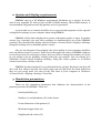
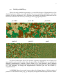
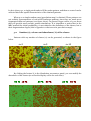
1
SIMMAP 2.0
Landscape categorical spatial patterns
simulation software
USER’S MANUAL
(May 2003)
Santiago Saura
ETSI Montes
Universidad Politécnica de Madrid
Ciudad Universitaria s/n
28040 Madrid
Spain
E-mail: [email protected]
This manual, software and related information can be downloaded from:
http://www2.montes.upm.es/personales/saura
INDEX
1. About SIMMAP
2
2. System and display requirements
3
3. Simulation parameters
3
4. Display and save options
11
5. Spatial pattern indices
13
6. Limitations and known errors
19
7. Where has been SIMMAP used?
21
2
1. About SIMMAP
SIMMAP is the result of implementing the modified random clusters (MRC
hereafter) simulation method. This method provides more general and realist results than
other commonly used landscape models, as has been described in the paper by Saura and
Martínez-Millán (2000), which is referenced below. The MRC method generates
categorical (thematic) landscape spatial patterns in raster format (grid-based data).
SIMMAP is distributed without charge for non-commercial use, with the only
condition of citing the following two references in any document or work in which
SIMMAP is used:
- Saura, S. and J. Martínez-Millán. 2000. Landscape patterns simulation with a
modified random clusters method. Landscape Ecology 15 (7): 661-678.
- Saura, S. 1998. Simulación de mapas temáticos mediante conglomerados
aleatorios. Proyecto fin de carrera. Escuela Técnica Superior de Ingenieros de Montes.
Universidad Politécnica de Madrid. Madrid, Spain.
Users are asked to provide the author a brief description about the applications for
which SIMMAP is used.
The objective of this manual is to briefly describe how to use SIMMAP. The
necessary information for understanding the effects of the simulation parameters on the
MRC patterns is provided. Also, a concise description of the landscape pattern
configuration indices that are used to quantify the spatial characteristics of the simulated
patterns is included. Further details about the MRC method and its results can be found in
the paper by Saura and Martínez-Millán (2000), and are out of the scope of this document.
SIMMAP simulations are very low computational time consuming. In a standard PC
at 333 MHz, typical computational times are less than one second for 200x200 pixels
patterns, around 2 seconds for 400x400 images, and around 4 seconds for 800x800 pixels
landscapes.
SIMMAP patterns may be used for many purposes in different fields such as
landscape ecology, remote sensing, spatial statistics, simulation and computer graphics,
etc (see section 7). The author hopes that this software is useful for your particular
application, and looks forward to hear about it.
SIMMAP is provided “as-is”, without warranty of any kind. The user assumes all the
responsibility for the accuracy and suitability of this program for a specific application.
Note that a point (and not a comma) should be set as your decimal separator in the
regional configuration settings of your computer when using SIMMAP.MAP
3
2. System and display requirements
SIMMAP runs on a PC-Windows environment (Windows 95 or newer). It can be
used in any standard PC with at least 16 MB of RAM memory. More RAM memory is
recommended if big patterns with big patches are to be generated.
A point (and not a comma) should be set as your decimal separator in the regional
configuration settings of your computer when using SIMMAP.
SIMMAP will be better displayed in screens of 800x600 pixels or more. In smaller
screens (e.g. 640x480) you may have problems to simultaneously see all the SIMMAP
windows. You can adjust the display size in Windows->Control Panel->Display->Settings,
fixing the Desktop area to 800x600 pixels or more.
Also, for an adequate colours display, the colour palette in your computer should be
set to 16 million colours (or more). If the icon in the upper left corner of SIMMAP windows
is not shown in brown and green colours, then you need to change the number of colours
in your palette (you are probably working with only 256 colours). You can change it in
Windows->Control Panel->Display->Settings, fixing the Colour palette to 16 million
colours (true colour, 16 bits) or more.
SIMMAP has been designed to run with small fonts (96 dpi). Big fonts (120 dpi) will
also work fine. Other font sizes out of this range (96-120 dpi) have not been tested, but
they are very rarely used. You may fix the font sizes in your computer in Windows>Control Panel->Display->Settings->Font Size.
3. Simulation parameters
There are five simulation parameters that influence the characteristics of the
patterns generated by SIMMAP. These are:
-
Initial probability (p)
-
Number (n) and abundance (%) of the classes
-
Linear dimension of the pattern (L)
-
Minimum mapped unit (m)
-
Neighbourhood criteria (N)
4
The controls for all these parameters are included in the Simulation parameters
panel located in the upper part of the SIMMAP 2.0 window.
A very wide variety of spatial categorical patterns can be obtained by adequately
varying these simulation parameters, as described below.
First of all, it is important to note that SIMMAP is based on a stochastic simulation
method. That is, any number of patterns can be obtained for the same values of the
simulation parameters, which differ in the exact location of classes in the pattern (each
generated image is really unique!), but are similar in their overall spatial structure and
appearance. This is illustrated in the figure below.
5
3.1.
Initial probability p
This is the main simulation parameter. p controls the degree of fragmentation of the
obtained patterns. When p is small, patches are more numerous and smaller, and thus
patterns are more fragmented. As p increases, the number of patches decreases and its
mean and maximum size increase, resulting in more aggregated patterns.
p=0.58
p=0.55
p=0.50
p=0.4
p=0.2
p=0
As shown in the figure above, the increase in pattern aggregation is not linear, but
more rapid as p is nearer a certain value, the percolation threshold (pc). pc 0.5928 for the
default 4-neigbourhood criterion. Other values of pc are obtained when different
neighbourhood criteria are used; however, as will be described later, for most simulations
it is not necessary to change the neighbourhood criterion (just use the default 4neighbourhood).
In SIMMAP there is no need to use values of p bigger than pc. All the variety of
patterns can be obtained with p<pc by adequately fixing the simulation parameters values.
6
In fact, when p>pc, a single patch tends to fill the entire pattern, and then no control can be
achieved about the spatial characteristics of the obtained patterns.
When p=0 a simple random map (percolation map) is obtained. These patterns are
not realistic representations of real-world landscape patterns, since they are much more
fragmented than real patterns (see figure above). In general, bigger values of p are those
that will provide more realistic pattern simulations. It is important to notice that in the
MRC method the initial probability p is not related to the abundance of the classes, but to
their fragmentation degree (this is opposite to what occurs in percolation maps).
3.2.
Number (n), colours and abundance (%) of the classes
Patterns with any number of classes (n) can be generated, as shown in the figure
below.
n=2
n=5
n=10
By clicking the button % in the Simulation parameters panel, you can modify the
abundance of the classes (as well as the display colour for each class).
90 % 10 %
50 %
50 %
20 %
80 %
7
To modify the percent of total area to be occupied by each of the classes, you have to
input the adequate values for each of the classes in the Class weights edit box. You may
enter any value bigger than 0. SIMMAP internally normalises the weight values (wi) that
are introduced by the user and converts them to abundance probabilities (a i), so that their
sum equals 1, as follows:
ai 
wi
k n
w
k 1
k
where ai and wi are respectively the abundance probability and weight
corresponding to class i, and n is the total number of classes in the pattern. For example, if
you introduce the weights of 25 and 50 in a two-classes pattern, SIMMAP will assign 0.33
and 0.67 as the abundance probabilities for each of the classes.
SIMMAP assigns classes to the patches in the pattern in a probabilistic manner; that
is, ai is the probability that class i is assigned to a given patch in the pattern (whatever its
size). In many cases, the obtained class abundance (actual percent of the pattern area
occupied by each of the classes in the final image) will be very close to 100·ai (the
“requested” abundance). However, if high values of the initial probability p are used, big
patches will be generated and it may be more problematic to obtain the desired classes
abundances. In particular, if p>pc a patch will tend to fill the landscape occupying, for
example, 80% of total area. In this case it will be impossible to obtain a 3-classes pattern
with each of them occupying 33% of the area (the class to which the big patch is assigned
will occupy at least 80%). Also, if p is near to pc big patches will appear that may make
difficult to obtain the desired abundances. Consider for illustrative purposes a hypothetical
pattern with 10 patches, each of them occupying 10% of total area. Suppose that the user
wants class 1 to occupy 20% of total area. Since classes are assigned randomly, 1 (10%) or 2
(20%) or 3 (30%) patches (etc.) may be assigned, with a certain probability, to class 1, and
is not ensured that the desired 20% will be obtained in a particular MRC simulation. These
effects are less pronounced the smaller the percent of total area occupied by the individual
patches in the pattern (i.e. the lower p is and the bigger L is). So, if you need to obtain a
more accurate class abundance increase L and/or decrease p.
The actual class abundance that is obtained in the generated MRC patterns is shown
in the Indices window, in the index PL (percent of pattern area occupied by each of the
classes).
On the right of the Change abundances and colours window, the colour
corresponding to each of the classes is displayed. Just press the button Change below Class
colour, and select the colour with which you want that class to be displayed, or specify it in
detail by its RGB components (by pressing Define custom colours).
8
3.3.
Map linear dimension (L)
Map linear dimension (L) is simply the length (in pixels) of the side of the square
pattern to be obtained. Thus, the total number of pixels in the resultant patterns is LxL.
L=300
L=200
3.4.
Minimum mapped unit (m)
m is the minimum mapped unit (size of the smallest patch) to appear in the MRC
patterns. The default (and minimum value) is 1 (patches comprised by a single pixel will
exist). Varying m you can simulate landscape patterns corresponding to different scales or
different degrees of detail in the interpretation of remotely sensed images.
m=1
m=20
m=50
9
m=1
3.5
m=20
m=50
Neighbourhood criterion (N)
This parameter is the last one you may want to vary, once you previously
understood and tested the influence of the previous ones. In general there is no need to
vary this parameter. You only need to change the neighbourhood criterion if patterns with
anisotropy (with patches oriented in a certain dominant direction) are to be obtained.
This parameter controls how patches (clusters, strictly speaking) are built from
initially random binary patterns (see the paper by Saura and Martínez-Millán (2000) for
further details). For each neighbourhood criterion a different value of the percolation
threshold (pc) is obtained (pc 0.5928 for the default 4-neigbourhood criterion).
A neighbourhood criterion is defined by entering, for each of the 8 neighbour cells,
the probabilities of being considered as belonging to the same cluster that the central pixel
(marked by an X in the figure below). For example, see below the definition of the 4neighbourhood criteria (the default used by SIMMAP). Other symmetric neighbourhood
criteria can be defined, as is the case of the 8-neighbourhood criteria (see below). For this
8-neighbourhood criterion, the percolation threshold (pc) is around 0.41. However,
changing to the 8-neighbourhood criteria does not provide a significant increase in the
variety of the obtained patterns (Saura 1998). However, there are neighbourhood criteria
that do provide different patterns than those that can be obtained with the 4neighbourhood rule; these are the asymmetrical neighbourhood criteria (both 4 and 8neighbourhood are symmetrical rules). These asymmetric criteria generate patterns with
anisotropy, that is, with patches oriented in a certain dominant direction (e.g. the
horizontal and the two diagonal criteria shown below).
0 1 0
1
1
0 1 0
1 1 1
1
1
1 1 1
0 1 1
1
1
1 1 0
4-Neighbourhood
8-Neighbourhood
Diagonal
0 0.2 1
0.2
0.2
0 0 1
1
1
1 0.2 0
0 0 1
Diagonal+
Horizontal
10
When the neighbourhood criteria is changed also the percolation threshold (pc)
changes, and thus the value of p that generates a certain pattern fragmentation degree is
also different. In general, wider neighbourhood criteria produce more aggregated patterns
for the same value of the initial probability p (e.g. the 8-neighbourhood is a wider criteria
than the 4-neighbourhood); so, pc is reduced and the range of p values interesting for the
simulations is also shortened. The opposite occurs when more restrictive criteria are used
(e.g. the “Diagonal+” criterion in the figure above is more restrictive than the “Diagonal”
one). These effects are illustrated in the p values used in the simulated patterns in the
figure below.
4-neighbourhood (p=0.55)
Diagonal (p=0.45)
8-neighbourhood (p=0.37)
Diagonal+ (p=0.7)
Horizontal (p=0.47)
To change the neighbourhood criterion, click the N button in the SIMMAP 2.0
window. You can just choose one of the common ones that are already predefined in
SIMMAP (the five criteria that are described and illustrated above) by selecting the option
Common criteria. Or you can specify in detail the criterion by entering the neighbourhood
probability values in each of the 8 adjacent cells (selecting the option Other criteria).
11
4. Display and save options
4.1.
Displaying the MRC patterns
These options (located in the Display options panel of the SIMMAP 2.0 window)
control how the generated patterns are displayed in your computer screen. The colours of
the classes to be used for the display are selected in the Classes abundance and colours
window (after pressing the % button in the Simulation parameters panel), as described in
section 3.2.
If you select the Window to pattern option, the MRC patterns will be displayed in a
window with the same number of pixels than the MRC patterns. On the contrary, the
Pattern to window option will fit the MRC simulated patterns in a window of specified
linear dimension (which is entered in the edit box below the Pattern to window option).
This allows enlarging or reducing the original MRC patterns when they are displayed. This
may be also useful to display MRC patterns bigger than the screen size.
L=400 displayed in
400x400 pixels window
(1 to 1 display scale)
L=400 displayed
in 200x200
pixels window (reduced)
12
L=200 displayed in
400x400 pixels window (enlarged)
L=200 displayed in
200x200 pixels window
(1 to 1 display scale)
If the Multiple windows option is enabled, each new pattern that is generated is
displayed in a new (different) display window. Thus, you get as many windows as
simulations you make. If your computer RAM memory is running out (normally this
should not be a problem), or if you do not feel comfortable with too many windows, disable
this option; each new pattern will be then displayed in the same display window, and thus
previous simulations will be lost.
4.2.
Saving the MRC patterns
The MRC patterns generated by SIMMAP can be saved in image files (“bmp“
format), which may be imported into other remote sensing, GIS or image processing
programmes if necessary. Just press the button Save in the upper left part of the windows
in which each of the generated patterns is displayed; a save dialogue will appear where you
can specify the location and name of the file where the corresponding pattern will be saved.
The option selected to display the MRC patterns has an influence in the
characteristics of the saved image file. When you save a pattern that has been generated
with the Window to pattern option, the resultant image file will have the same resolution
(number of pixels) than the original MRC pattern. This is highly recommended, as you are
13
saving the real spatial information provided by the MRC method (1:1 scale). On the
contrary, if the Pattern to window option is selected, what you are saving is not the real
MRC data but an enlargement or reduction as modified by the computer to show the
pattern in a display window of a given size. You should avoid this if further quantitative
analysis (not just for display or graphical purposes) are to be done with the simulated MRC
landscapes. If you want to save in “bmp” files MRC patterns bigger than your screen size
(and still retain the original MRC spatial data), just generate the simulations with the
Window to pattern option selected; you will not be able to see the entire obtained pattern
in your screen, but the Save button will always be visible in the upper left corner of the
pattern window; just press Save and you will store the entire generated pattern in the
image file (even if you can not see it completely in your screen).
5. Spatial pattern indices
Several landscape pattern configuration indices are computed on the MRC patterns.
This allows quantifying the spatial characteristics of the simulated landscapes, as well as
their comparison with real-world pattern data.
It is not the purpose of the author to give a description of the background and
behaviour of these pattern indices. This is out of the scope of this manual, and can be
found in the landscape ecology and spatial pattern analysis literature, where these indices
are frequently used. Only a brief description of the indices is provided, so that no
ambiguity exists about how they are calculated and what are they really measuring.
SIMMAP is itself a good tool to understand how these indices behave when varying pattern
characteristics (just change simulation parameters and see how indices vary!).
Two important definitions affect how indices are calculated and thus the obtained
values of the pattern indices:
- Definition of patch. A patch is defined in SIMMAP according to the 4neighbourhood rule (this has no relation with the neighbourhood criterion simulation
parameter; whatever the value of that simulation parameter the patches are always defined
in the same way to compute the indices values!). This 4-neighbourhood rule considers as
belonging to the same patch those pixels that are adjacent horizontal or vertically, but not
along the diagonals. Many authors use this definition of patch, although some others use
the 8-neighbourhood rule; indices values obtained with each of these two rules are not
directly comparable. The definition of patch affects many of the indices that are described
below (NP, PD, MPS, SMPS, AWMPS, PSSD, LPI, NPI, PPI, IA, MSI, AWMSI, PAFD, PC),
although the calculation of some others does not require previous identification of patches
on the pattern (EL, ED, IEL, IED).
- Definition of perimeter. SIMMAP defines perimeter as the length of the patch
outer boundary. So, edges defined by small islands embedded inside the patch are not
included in the definition of perimeter. However, many programmes that are commonly
used for the computation of landscape indices (e.g. FRAGSTATS) do not differentiate
between the inner edges and the true perimeter, including both concepts in the computed
“perimeter”. Both definitions of perimeter provide different values of the perimeter-
14
dependent indices that are described below (in general, higher values of MSI, AWMSI,
PAFD and PC are obtained if inner edges are included). Probably a more adequate
measurement of pattern shapes is obtained when inner edges are not included in patch
perimeters. However, for comparability purposes, SIMMAP includes the possibility of
obtaining the values of the indices corresponding to any of these two definitions. Just click
in the Include inner edges in perimeter option in the Indices window to view the indices
values according to the desired definition (if this option is activated, inner edges are also
included in the patch perimeters).
All the indices are computed both at the class (only patches that belong to a certain
class are considered in the calculation of the indices) and landscape-level (all patches in
the pattern are considered, independently of which class they belong to). The indices
values for each of the classes and for the entire simulated landscape are shown in the
Indices window, which is located by default at the right of the SIMMAP main window. All
these indices are calculated only if the option Indices (located under the Simulate button,
in the lower right part of SIMMAP main window) is activated.
One index is presented only at the class-level; this is PL (percent of total pattern
area occupied by a certain class).
5.1. Number of patches and size indices
NP : Number of Patches in the class or landscape.
PD : Patch Density (%). Is a normalised way to express NP, and is here calculated
as:
PD  100 
NP
L2
where NP is the number of patches (in the class or landscape) and L2 is the
total number of pixels in the entire landscape. L2 is also the maximum number of
patches (defined with the 4-neighbourhood rule) that may appear in raster
landscape data.
MPS : (Arithmetic) Mean Patch Size (expressed in pixels).
i  NP
MPS 
a
i 1
i
NP
where ai is the size (area, in pixels) of each of the patches in the class or
landscape.
15
SMPS : Squared Mean Patch Size (expressed in pixels). Is an alternative measure of
central tendency that gives smaller weight to the smaller patches in the pattern.
i  NP
a
SMPS 
i 1
2
i
NP
where ai is the size (area, in pixels) of each of the patches in the class or
landscape.
AWMPS : Area Weighted Mean Patch Size (expressed in pixels). Like MPS or
SMPS, but giving even less weight to the small patches in the pattern when computing the
mean size. It is calculated according to the following expression:
i  NP
AWMPS 
a
i 1
2
i
L2
PSSD : Patch Size Standard Deviation.
i  NP
PSSD 
 MPS  a 
2
i
i 1
NP
The values of PSSD, MPS and SMPS are related by the following simple expression:
SMPS 2  MPS 2  PSSD 2
LPI : Largest Patch Index (%). Is the percent of the total class or landscape area
occupied by the largest patch in the class or landscape.
NPI : Number of Patches with Islands. Islands are holes or inner patches embedded
inside bigger ones. NPI is just the total number of patches in the class or landscape which
have islands inside them.
PPI : Percent of Patches with Islands (%).
16
PPI  100 
NPI
NP
IA : Islands Area (%). Is the sum of the areas of the island patches (those that are
embedded inside a bigger patch) expressed as a percentage of the total pattern area. At the
class-level, IA sums the areas of the islands that are embedded in the patches of a given
class (not the areas of islands belonging to that class embedded in other patches).
5.2. Edge indices
EL : Edge Length (expressed in pixel sides). An edge is defined as a shared side
between two pixels that belong to different classes. Edges defined by map border are not
included.
ED : Edge Density (%). Expressed as percentage of the maximum edge length that
can appear in raster patterns of linear dimension L. It is simple to demonstrate that 2·L·(L1) is the maximum edge length that can appear in raster landscape data of linear
dimension L.
ED  100
EL
2·L·L  1
IEL : Inner Edge Length (expressed in pixel sides). Inner edges are defined as those
edges that are completely surrounded by pixels of the same class. Thus, it measures the
presence of holes or islands in the patches in the pattern.
IED : Inner Edge Density (%). Like ED, it is expressed as a percentage with respect
to the maximum edge length that can appear in grid based data (2·L·(L-1)). However, EL 
IEL and, in general, values for IED much nearer to 0 than to 100 are clearly to be expected.
IED  100
IEL
2·L·(L  1)
5.3. Shape indices
The following three indices (MSI, AWMSI and PAFD) intend to measure the
complexity, irregularity or elongation of the shapes in the pattern, taking higher values the
more convoluted and elongated the shapes are.
MSI : Mean Shape Index. Its minimum value (for perfectly squared patches shapes)
is 1.
17
i  NP
pi
ai
i 1
MSI 
NP
4
AWMSI : Area Weighted Mean Shape Index. It is similar to MSI (its minimum
value is also 1) but uses patch area as a weighting factor because larger patches are
assumed to have more importance for overall landscape structure.
i  NP
AWMSI 
pi
·ai
ai
 4·
i 1
i  NP
a
i 1
i
i  NP

p·
i 1
i
ai
i  NP
4·  ai
i 1
PAFD : Perimeter-Area Fractal Dimension. It derives from fractal theory. It can be
demonstrated that the perimeters (p) and areas (a) of a set of self-similar shapes obey the
following relation:
p  k a
PAFD
2
where k is a constant and PAFD is the Perimeter-Area Fractal Dimension
(theoretically ranging from 1 to 2) of the set of similar shapes. Assuming self-similarity in
the patches shapes, and taking logarithms in both sides of this equation, PAFD is
estimated as twice the slope of the fitted line of perimeters (p) versus areas (a) of each of
the patches of the class or landscape. However, the least-squares regression can be done in
two ways:
ln p  k ' 
PAFD
 ln a
2
(1)
(perimeter as dependent variable. PAFD equals twice the slope of the regression
line)
ln a  k '' 
2
 ln p
PAFD
(2)
(area as dependent variable. PAFD equals twice the inverse of the slope of the
regression line).
18
Both expressions yield (slightly) different values for PAFD, and there is not a special
reason why one should be preferable to the other. You may find PAFD calculated in any of
these two ways, depending on the author or the software used for its computation. If the
option Perimeter as dependent variable in the Indices window is enabled, PAFD is
computed according to expression 1; if it is disabled, then patch area is used as the
dependent variable in the regression (expression 2).
The coefficient of determination of this regression (R2) may be considered as an
indicator of self-similarity in the analysed pattern, and is included in the indices window
next to the PAFD value. Values of R2 bigger than 0.9 are very frequently obtained in
landscape patterns. The value of R2 is not affected by which of the two previous
expressions is used in the regression.
As estimated by regression techniques, PAFD needs a sufficient number of patches
in the pattern to be adequately estimated. When values outside the theoretical range of
variation for PAFD (1 to 2) or R2 (–1 to 1) are obtained, “NV” is displayed in the
corresponding boxes in the Indices window.
5.4. Other indices
PC : Patch Cohesion. This index was developed by Nathan H. Schumaker and,
according to the simulation model he developed, it correlates better with animal
populations dispersal success than any other of the commonly used landscape pattern
indices. It is calculated as:
i  NP

pi


PC  1  i  NPi 1

pi · ai
 
i 1

  1  1
·1  
  L

where pi and ai are the perimeter and area of each of the patterns in the class or
landscape, and L is pattern linear dimension (in pixels).
PC value is minimum (PC=0) when all patches of habitat are confined to single
isolated pixels, and maximum (PC=1) when every pixel is included in a single patch that
fills the landscape.
19
5.5. About the comparison of the indices values calculated with SIMMAP
and FRAGSTATS
Some users may wish to make the indices values given by SIMMAP equal to those
provided by a commonly used software like FRAGSTATS. If this is the case, select the
option Include inner edges in perimeter and deselect the option Perimeter as dependent
variable. Also, compute the indices in the raster version of FRAGSTATS with the 4neighbourhood rule (i.e. do not use diagonals in patch finding). This way the same values
of NP, LPI, MSI, AWMSI, PAFD (the initials for this index are DLFD in FRAGSTATS) and
PL (the initials for this index are %LAND in FRAGSTATS) will be obtained with both
programmes. Some other indices are also comparable in SIMMAP and FRAGSTATS,
although they require some slight modifications according to the following expressions:
MPS
SMP
MPS FRG

A pix
PSSD SMP 
PSSD FRG
A pix
PD SMP  PD FRG  Apix
EL
SMP

ELFRG
10000  A pix
ED SMP  ED FRG 
L  A pix
50  L  1
where ISMP and IFRG are respectively the values of the index I calculated by SIMMAP
and FRAGSTATS, and Apix is the area (in hectares) of the pixel, which is used by
FRAGSTATS to compute the values of those indices.
The rest of the indices that are calculated by SIMMAP are not computed by
FRAGSTATS or vice versa.
6. Limitations and known errors
SIMMAP has been checked in detail in order to avoid errors. Thus hopefully no
important problems should appear. However, it is possible that users find some bugs that
were not detected before. Help in reporting bugs is appreciated.
Some issues that may arise when using SIMMAP with non-adequate display settings
have been described in section 2 (System and display requirements).
20
Note that a point (and not a comma) should be set as your decimal separator in the
regional configuration settings of your computer when using SIMMAP.MAP
You may suffer from lack of RAM memory if you are generating very large patterns
with large patches and your computer RAM is not very large (e.g. only 16 MB). If this is the
case, try not to use p values over the percolation threshold (usually 0.5928, for the default
4-neighbourhood criterion) if you are generating big MRC patterns (big L), especially
considering that these values are not of particular interest in the MRC method. Also, if you
generate too many patterns (i.e. open too many display windows simultaneously) you may
have problems with your RAM memory, even if the patterns are not really big; however,
this should not happen frequently, even in computers with only 16 MB RAM. If so, disable
the option Multiple windows in the SIMMAP 2.0 main window; this way only one display
window will be presented in your screen, showing the last pattern you generated and
making less use of your RAM memory (note that then previously generated patterns will be
lost). You can notice that you are running out of RAM memory if your computer is making
an intensive use of the hard disk when generating the MRC patterns (if enough RAM is
available, SIMMAP does not need at all to use your hard disk; otherwise Windows may use
the space in your hard disk to place the data that can not be located in your RAM memory.
This will cause simulations to slow down).
Several simulation and display parameters have limitations in their maximum
values in SIMMAP 2.0. The limitations are the following:
- Maximum pattern linear dimension (L): 2000 pixels.
- Maximum minimum mapped unit (m): 99 pixels.
- Maximum number of classes (n): 29.
- Maximum display window linear dimension: 2000 pixels.
In what refers to the minimum mapped unit, SIMMAP will be able to remove a
maximum of 160.000 small patches (patches smaller than the specified minimum mapped
unit). Only in some combinations of simulation parameters values (which are not very
reasonable) this limitation may be exceeded. For example, if you simulate a pattern for
p=0 and L=1500, and in addition you want to obtain m=90, there will be too many patches
to remove from the original pattern (in fact probably all the patches will be of size smaller
than m, and that’s quite a lot!). If this happens, SIMMAP will show a message box saying
“Too many patches smaller than m pixels to remove! Requested pattern cannot be
successfully simulated”. In this case it is suggested to decrease m or L and/or increase p.
It is expected that these maximum values are more than enough for the majority of
the applications. If not, a version of SIMMAP with a higher maximum value for some of
these parameters may be provided, if possible, to those interested.
21
7. Where has been SIMMAP used?
SIMMAP and the modified random clusters method have been used as a key part of
the analyses in the following papers published in international SCI journals (Science
Citation Index), where you can find examples and ideas on the application of this software
for various purposes:
Díaz-Varela, E.R., Marey-Pérez, M.F., Álvarez-Álvarez, P. 2009. Use of simulated
and real data to identify heterogeneity domains in scale-divergent forest landscapes. Forest
Ecology and Management 258: 2490-2500.
Peng, J., Wang, Y., Zhang, Y., Wu, J., Li, W., Li, Y. 2010. Evaluating the
effectiveness of landscape metrics in quantifying spatial patterns. Ecological Indicators 10:
217-223.
Shuangcheng, L., Qing, C., Jian, P., Yanglin, W. 2009. Indicating landscape
fragmentation using L-Z complexity. Ecological Indicators 9: 780-790.
Hagen-Zanker, A. 2009. An improved Fuzzy Kappa statistic that accounts for spatial
autocorrelation. International Journal of Geographical Information Science 23: 61-73.
Estrada-Peña, A., Acevedo, P., Ruiz-Fons, F., Gortázar, C., de la Fuente, J. 2008.
Evidence of the importance of host habitat use in predicting the dilution effect of wild boar
for deer exposure to Anaplasma spp. PLoS ONE 3(8): e2999.
Hufkens, K., Bogaert, J., Dong, Q.H., Lu, L., Huang, C.L., Ma, M.G., Che, T., Li, X.,
Veroustraete, F., Ceulemans, R. 2008. Impacts and uncertainties of upscaling of remotesensing data validation for a semi-arid woodland. Journal of Arid Environments 72: 14901505.
Millington, J., Romero-Calcerrada, R., Wainwright J., Perry, G. 2008. An agentbased model of Mediterranean agricultural land-use/cover change for examining wildfire
risk. Journal of Artificial Societies and Social Simulation 11: 4.
La Sorte, F.A., Hawkins, B.A. 2007. Range maps and species richness patterns:
errors of commission and estimates of uncertainty. Ecography 30: 649-662.
Li, X.Z., He, H.S., Bu, R.C., Wen, Q.C., Chang, Y., Hu, Y.M., Li, Y.H. 2005. The
adequacy of different landscape metrics for various landscape patterns. Pattern
recognition 38 (12): 2626-2638.
Shen, W.J., Jenerette, G.D., Wu, J.G., Gardner, R.H. 2004. Evaluating empirical
scaling relations of pattern metrics with simulated landscapes. Ecography 27 (4): 459-469.
22
Li, X.Z., He, H.S., Wang, X.G., Bu, R.C., Hu, Y.M., Chang, Y. 2004. Evaluating the
effectiveness of neutral lanscape models to represent a real landscape. Landscape and
Urban Planning 69 (1): 137-148.
Saura, S. 2002. Effects of minimum mapping unit on land cover data spatial
configuration and composition. International Journal of Remote Sensing 23 (22): 48534880.
Saura, S., Martínez-Millán, J. 2001. Sensitivity of landscape pattern metrics to map
spatial extent. Photogrammetric Engineering and Remote Sensing 67 (9): 1027-1036.