Download IDEAS User Manual 4.0 - Department of Flow and Image Cytometry

Image Data Exploration and Analysis Software
User’s Manual
Version 4.0 December 2010
Amnis Corporation
2505 Third Avenue, Suite 210
Seattle, WA 98121
Phone: 206-374-7000
Toll free: 800-730-7147
www.amnis.com
Patents and Trademarks
Amnis Corporation's technologies are protected under one or more of the following
U.S. Patent Numbers: 6211955; 6249341; 6473176; 6507391; 6532061; 6563583;
6580504; 6583865; 6608680; 6608682; 6618140; 6671044; 6707551; 6,763,149;
6778263; 6875973; 6906792; 6934408; 6947128; 6947136; 6975400; 7006710;
7009651; 7057732; 7079708; 7087877; 7190832; 7221457; 7286719; 7315357;
7450229; 752275; 7567695; 7610942; 7634125; 7634126; 7719598. Additional U.S.
and corresponding foreign patent applications are pending.
Amnis, the Amnis logo, INSPIRE, IDEAS, and ImageStream, are registered or
pending U.S. trademarks of Amnis Corporation. All other trademarks are
acknowledged.
End User License Agreement
AMNIS CORPORATION SOFTWARE LICENSE AGREEMENT
PLEASE READ THE FOLLOWING TERMS AND CONDITIONS
CAREFULLY BEFORE DOWNLOADING, INSTALLING OR USING THE
SOFTWARE OR ANY ACCOMPANYING DOCUMENTATION
(COLLECTIVELY, THE “SOFTWARE”).
THE TERMS AND CONDITIONS OF THIS SOFTWARE LICENSE
AGREEMENT (“AGREEMENT”) GOVERN USE OF THE SOFTWARE
UNLESS YOU AND AMNIS CORPORATION (“AMNIS”) HAVE EXECUTED
A SEPARATE AGREEMENT GOVERNING USE OF THE SOFTWARE.
Amnis is willing to license the Software to you only upon the condition that you
accept all the terms contained in this Agreement. By clicking on the “I accept” button
below or by downloading, installing or using the Software, you have indicated that
you understand this Agreement and accept all of its terms. If you are accepting the
terms of this Agreement on behalf of a Company or other legal entity, you represent
and warrant that you have the authority to bind that Company or other legal entity to
the terms of this Agreement, and, in such event, “you” and “your” will refer to that
Company or other legal entity. If you do not accept all the terms of this Agreement,
then Amnis is unwilling to license the Software to you, and you must return the
Software to Amnis for a full refund, if you have paid for the license to the Software, or,
if Amnis has made the Software available to you without charge, you must destroy all
copies of the Software. Your right to return the Software for a refund expires 30 days
after the date of purchase.
1.Grant of License. Conditioned upon your compliance with the terms and
conditions of this Agreement, Amnis grants you a non-exclusive and non-transferable
license to Execute (as defined herein) the executable form of the Software on a single
computer, solely for your internal business purposes. You may make a single copy of
the Software for backup purposes, provided that you reproduce on it all copyright and
other proprietary notices that are on the original copy of the Software. Amnis reserves
all rights in the Software not expressly granted to you in this Agreement. For purposes
of this Agreement, “Execute” and “Execution” means to load, install, and run the
Software in order to benefit from its functionality as designed by Amnis.
2.Restrictions. Except as expressly specified in this Agreement, you may not: (a) copy
(except in the course of loading or installing) or modify the Software, including but
not limited to adding new features or otherwise making adaptations that alter the
functioning of the Software; (b) transfer, sublicense, lease, lend, rent or otherwise
distribute the Software to any third party; or (c) make the functionality of the Software
available to multiple users other than the users of the single computer for which it is
licensed through any means, including but not limited to uploading the Software to a
network or file-sharing service or through any hosting, application services provider,
service bureau, software-as-a-service (SaaS) or any other type of services. You
acknowledge and agree that portions of the Software, including but not limited to the
source code, file formats, and the specific design and structure of individual modules or
programs, constitute or contain trade secrets of Amnis and its licensors. Accordingly,
you agree not to disassemble, decompile or reverse engineer the Software or data files,
in whole or in part, or permit or authorize a third party to do so, except to the extent
such activities are expressly permitted by law notwithstanding this prohibition.
3.Ownership. The copy of the Software is licensed, not sold. You own the media on
which the Software is recorded, but Amnis retains ownership of the copy of the
Software itself, including all intellectual property rights therein. The Software is
protected by United States copyright law and international treaties. You will not
delete or in any manner alter the copyright, trademark, and other proprietary rights
notices or markings appearing on the Software as delivered to you.
4.Term. The license granted under this Agreement remains in effect for a period of 75
years, unless earlier terminated in accordance with this Agreement. You may
terminate the license at any time by destroying all copies of the Software in your
possession or control. The license granted under this Agreement will automatically
terminate, with or without notice from Amnis, if you breach any term of this
Agreement. Upon termination, you must at Amnis’ option either promptly destroy or
return to Amnis all copies of the Software in your possession or control.
5.Limited Warranty. Amnis warrants that, for thirty (30) days following the date of
purchase (or delivery, if Amnis has made the Software available to you without
charge), the Software will perform in all material respects in accordance with the
Documentation. As your sole and exclusive remedy and Amnis’ entire liability for any
breach of this limited warranty, Amnis will at its option and expense promptly correct
or replace the Software so that it conforms to this limited warranty. Amnis does not
warrant that the Software will meet your requirements, that the Software will operate
in the combinations that you may select for Execution, that the operation of the
Software will be error-free or uninterrupted, or that all Software errors will be
corrected. The warranty set forth in this Section 5 does not apply to the extent that
Amnis provides you with the Software (or portions of the Software) for beta,
evaluation, testing or demonstration purposes.
6.DISCLAIMER. THE LIMITED WARRANTY SET FORTH IN SECTION 5
IS IN LIEU OF AND AMNIS EXPRESSLY DISCLAIMS ALL OTHER
WARRANTIES AND CONDITIONS, EXPRESS OR IMPLIED, INCLUDING
BUT NOT LIMITED TO ANY IMPLIED WARRANTIES AND CONDITIONS
OF MERCHANTABILITY, FITNESS FOR A PARTICULAR PURPOSE AND
NONINFRINGEMENT, AND ANY WARRANTIES AND CONDITIONS
ARISING OUT OF COURSE OF DEALING OR USAGE OF TRADE. NO
ADVICE OR INFORMATION, WHETHER ORAL OR WRITTEN,
OBTAINED FROM AMNIS OR ELSEWHERE WILL CREATE ANY
WARRANTY OR CONDITION NOT EXPRESSLY STATED IN THIS
AGREEMENT.
7.Limitation of Liability. AMNIS’ TOTAL LIABILITY TO YOU FROM ALL
CAUSES OF ACTION AND UNDER ALL THEORIES OF LIABILITY WILL
BE LIMITED TO THE AMOUNTS PAID TO AMNIS BY YOU FOR THE
SOFTWARE OR, IN THE EVENT THAT AMNIS HAS MADE THE
SOFTWARE AVAILABLE TO YOU WITHOUT CHARGE, AMNIS’ TOTAL
LIABILITY WILL BE LIMITED TO $100. IN NO EVENT WILL AMNIS BE
LIABLE TO YOU FOR ANY SPECIAL, INCIDENTAL, EXEMPLARY,
PUNITIVE OR CONSEQUENTIAL DAMAGES (INCLUDING LOSS OF
DATA, BUSINESS, PROFITS OR ABILITY TO EXECUTE) OR FOR THE
COST OF PROCURING SUBSTITUTE PRODUCTS ARISING OUT OF OR
IN CONNECTION WITH THIS AGREEMENT OR THE EXECUTION OR
PERFORMANCE OF THE SOFTWARE, WHETHER SUCH LIABILITY
ARISES FROM ANY CLAIM BASED UPON CONTRACT, WARRANTY,
TORT (INCLUDING NEGLIGENCE), STRICT LIABILITY OR OTHERWISE,
AND WHETHER OR NOT AMNIS HAS BEEN ADVISED OF THE
POSSIBILITY OF SUCH LOSS OR DAMAGE. THE FOREGOING
LIMITATIONS WILL SURVIVE AND APPLY EVEN IF ANY LIMITED
REMEDY SPECIFIED IN THIS AGREEMENT IS FOUND TO HAVE FAILED
OF ITS ESSENTIAL PURPOSE.
8.U.S. Government End Users. The Software and Documentation are “commercial
items” as that term is defined in FAR 2.101, consisting of “commercial computer
software” and “commercial computer software documentation,” respectively, as such
terms are used in FAR 12.212 and DFARS 227.7202. If the Software and
Documentation are being acquired by or on behalf of the U.S. Government, then, as
provided in FAR 12.212 and DFARS 227.7202-1 through 227.7202-4, as applicable,
the U.S. Government’s rights in the Software and Documentation will be only those
specified in this Agreement.
9.Export Law. You agree to comply fully with all U.S. export laws and regulations to
ensure that neither the Software nor any technical data related thereto nor any direct
product thereof are exported or re-exported directly or indirectly in violation of, or
used for any purposes prohibited by, such laws and regulations.
10.General. This Agreement will be governed by and construed in accordance with
the laws of the State of Washington, without regard to or application of conflict of
laws rules or principles. The United Nations Convention on Contracts for the
International Sale of Goods will not apply. You may not assign or transfer this
Agreement or any rights granted hereunder, by operation of law or otherwise, without
Amnis’ prior written consent, and any attempt by you to do so, without such consent,
will be void. Except as expressly set forth in this Agreement, the exercise by either
party of any of its remedies under this Agreement will be without prejudice to its other
remedies under this Agreement or otherwise. All notices or approvals required or
permitted under this Agreement will be in writing and delivered by confirmed
facsimile transmission, by overnight delivery service, or by certified mail, and in each
instance will be deemed given upon receipt. All notices or approvals will be sent to
the addresses set forth in the applicable ordering document or invoice or to such other
address as may be specified by either party to the other in accordance with this section.
The failure by either party to enforce any provision of this Agreement will not
constitute a waiver of future enforcement of that or any other provision. Any waiver,
modification or amendment of any provision of this Agreement will be effective only
if in writing and signed by authorized representatives of both parties. If any provision
of this Agreement is held to be unenforceable or invalid, that provision will be
enforced to the maximum extent possible, and the other provisions will remain in full
force and effect. This Agreement is the complete and exclusive understanding and
agreement between the parties regarding its subject matter, and supersedes all
proposals, understandings or communications between the parties, oral or written,
regarding its subject matter, unless you and Amnis have executed a separate agreement.
Any terms or conditions contained in your purchase order or other ordering document
that are inconsistent with or in addition to the terms and conditions of this Agreement
are hereby rejected by Amnis and will be deemed null.
11.Contact Information. If you have any questions regarding this Agreement, you
may contact Amnis at 2505 Third Avenue, Suite 210, Seattle, WA 98121.
DURING INSTALLATION, IF YOU AGREE TO THE FOREGOING TERMS
AND CONDITIONS AND DESIRE TO COMPLETE INSTALLATION OF
THE SOFTWARE, PLEASE CLICK THE “I ACCEPT” BUTTON.
OTHERWISE, PLEASE CLICK THE “I DO NOT ACCEPT” BUTTON AND
THE INSTALLATION PROCESS WILL STOP.
Disclaimers
The screen shots presented in this manual were created using the Microsoft®
Windows® XP operating system and may vary slightly from those created using other
operating systems.
The Amnis® ImageStream® cell analysis system is for research use only and not for
use in diagnostic procedures.
Technical Assistance
Amnis Corporation
2505 Third Avenue, Suite 210
Seattle, WA 98121
Phone: 206-374-7000
Toll free: 800-730-7147
www.amnis.com
Chapter 1:
Preface
1
How to use this manual . . . . . . . . . . . . . . . . . . . . . . . . . . . . . . . . . . . . . . . . . 1
What’s New in IDEAS 4.0 . . . . . . . . . . . . . . . . . . . . . . . . . . . . . . . . . . . . . . . 2
Chapter 2:
Setting Up the IDEAS® Application
5
Hardware and Software Requirements. . . . . . . . . . . . . . . . . . . . . . . . . . . . . . . 5
Hardware Requirements . . . . . . . . . . . . . . . . . . . . . . . . . . . . . . . . . . . . . 5
Software Requirements . . . . . . . . . . . . . . . . . . . . . . . . . . . . . . . . . . . . . . 5
Installing the IDEAS® Application. . . . . . . . . . . . . . . . . . . . . . . . . . . . . . . . . . 6
Setting Your Computer to Run the IDEAS® Application . . . . . . . . . . . . . . . . 6
Setting the Screen Resolution . . . . . . . . . . . . . . . . . . . . . . . . . . . . . . . . . 6
Viewing File Name Extensions . . . . . . . . . . . . . . . . . . . . . . . . . . . . . . . . 6
Copying the Example Data Files . . . . . . . . . . . . . . . . . . . . . . . . . . . . . . . 7
Viewing and Changing the Application Defaults . . . . . . . . . . . . . . . . . . . . . . . 8
Chapter 3:
Overview of the IDEAS® Application
9
Understanding the Data Analysis Workflow . . . . . . . . . . . . . . . . . . . . . . . . . . 10
Overview of compensation, analysis tools and file structure. . . . . . . . . . . . . . . 12
Data Acquisition and Compensation . . . . . . . . . . . . . . . . . . . . . . . . . . . 12
Data Analysis Tools . . . . . . . . . . . . . . . . . . . . . . . . . . . . . . . . . . . . . . . . 12
Interface of the IDEAS Application . . . . . . . . . . . . . . . . . . . . . . . . . . . . 13
Overview of the Data File Types . . . . . . . . . . . . . . . . . . . . . . . . . . . . . . 13
Raw Image File (.rif) .........................................................................14
Compensated Image File (.cif) ...........................................................14
Data Analysis File (.daf) .....................................................................14
Template (.ast) ...................................................................................15
Compensation Matrix File (.ctm) .......................................................15
Review of Data File Types ................................................................16
Chapter 4:
Getting Started with the IDEAS Application
17
Guided Analysis . . . . . . . . . . . . . . . . . . . . . . . . . . . . . . . . . . . . . . . . . . . . . . 18
Application Wizards . . . . . . . . . . . . . . . . . . . . . . . . . . . . . . . . . . . . . . . 18
Open File: .........................................................................................19
Display Properties: .............................................................................20
Apoptosis: .........................................................................................21
Cell Cycle - Mitosis ..........................................................................22
Co-localization ..................................................................................23
Internalization ...................................................................................24
Nuclear Localization ..........................................................................25
Shape Change ...................................................................................26
Building Blocks: . . . . . . . . . . . . . . . . . . . . . . . . . . . . . . . . . . . . . . . . . . 27
i
Advanced Analysis . . . . . . . . . . . . . . . . . . . . . . . . . . . . . . . . . . . . . . . . . . . . 29
The File Menu . . . . . . . . . . . . . . . . . . . . . . . . . . . . . . . . . . . . . . . . . . . 29
Opening a .rif file ..............................................................................29
Opening a .cif file ..............................................................................33
Opening a .daf file .............................................................................35
Merging .cif files ................................................................................36
Viewing Sample Information . . . . . . . . . . . . . . . . . . . . . . . . . . . . . . . . . 37
Overview of Compensation . . . . . . . . . . . . . . . . . . . . . . . . . . . . . . . . . 38
Creating a New Compensation Matrix File . . . . . . . . . . . . . . . . . . . . . . 40
Preview a compensation matrix . . . . . . . . . . . . . . . . . . . . . . . . . . . . . . . 48
Merging Raw Image Files . . . . . . . . . . . . . . . . . . . . . . . . . . . . . . . . . . . 49
Merging Compensated Image Files . . . . . . . . . . . . . . . . . . . . . . . . . . . . 50
Saving Data Files . . . . . . . . . . . . . . . . . . . . . . . . . . . . . . . . . . . . . . . . . . 51
Saving a Data Analysis File (.daf) ........................................................51
Saving a Compensated Image File (.cif) ..............................................52
Saving a Template (.ast) .....................................................................52
Creating Data Files from Populations .................................................52
Batch Processing . . . . . . . . . . . . . . . . . . . . . . . . . . . . . . . . . . . . . . . . . . 54
Chapter 5:
Using the Data Analysis Tools
59
Overview of the Data Analysis Tools . . . . . . . . . . . . . . . . . . . . . . . . . . . . . . . 59
Using the Image Gallery . . . . . . . . . . . . . . . . . . . . . . . . . . . . . . . . . . . . . . . . 60
Overview of the Image Gallery . . . . . . . . . . . . . . . . . . . . . . . . . . . . . . . 61
Setting the Image Gallery Properties . . . . . . . . . . . . . . . . . . . . . . . . . . . 64
Working with Individual Images . . . . . . . . . . . . . . . . . . . . . . . . . . . . . . 70
Creating Tagged Populations . . . . . . . . . . . . . . . . . . . . . . . . . . . . . . . . . 71
Using the Analysis Area . . . . . . . . . . . . . . . . . . . . . . . . . . . . . . . . . . . . . . . . 73
Overview of the Analysis Area . . . . . . . . . . . . . . . . . . . . . . . . . . . . . . . . 73
Creating Graphs . . . . . . . . . . . . . . . . . . . . . . . . . . . . . . . . . . . . . . . . . . 75
Creating Regions on Graphs . . . . . . . . . . . . . . . . . . . . . . . . . . . . . . . . . 80
Analyzing Images . . . . . . . . . . . . . . . . . . . . . . . . . . . . . . . . . . . . . . . . . 85
Adding Text to the Analysis Area . . . . . . . . . . . . . . . . . . . . . . . . . . . . . 88
Using the Statistics Area . . . . . . . . . . . . . . . . . . . . . . . . . . . . . . . . . . . . . . . . 89
Overview of the Statistics Area . . . . . . . . . . . . . . . . . . . . . . . . . . . . . . . 89
Viewing the Population Statistics . . . . . . . . . . . . . . . . . . . . . . . . . . . . . . 89
Viewing the Object Feature Values . . . . . . . . . . . . . . . . . . . . . . . . . . . . 92
Using the Mask Manager . . . . . . . . . . . . . . . . . . . . . . . . . . . . . . . . . . . . . . . 94
Overview of the Mask Manager . . . . . . . . . . . . . . . . . . . . . . . . . . . . . . 94
Creating New Masks with the Mask Manager . . . . . . . . . . . . . . . . . . . . 94
Example of Creating a Mask . . . . . . . . . . . . . . . . . . . . . . . . . . . . . . . . . 98
Viewing and Editing a Mask . . . . . . . . . . . . . . . . . . . . . . . . . . . . . . . . 100
Using the Feature Manager . . . . . . . . . . . . . . . . . . . . . . . . . . . . . . . . . . . . . 101
Overview of the Feature Manager . . . . . . . . . . . . . . . . . . . . . . . . . . . . 101
Creating New Features with the Feature Manager . . . . . . . . . . . . . . . . 103
Using the Population Manager . . . . . . . . . . . . . . . . . . . . . . . . . . . . . . . . . . 108
ii
Using the Region Manager . . . . . . . . . . . . . . . . . . . . . . . . . . . . . . . . . . . . . 111
Chapter 6:
Creating Reports and Exporting Data
113
Printing Reports. . . . . . . . . . . . . . . . . . . . . . . . . . . . . . . . . . . . . . . . . . . . . 113
Creating a Statistics Report Template . . . . . . . . . . . . . . . . . . . . . . . . . . . . . 116
Generating a Statistics Report using .daf Files. . . . . . . . . . . . . . . . . . . . . . . . 118
Exporting Data . . . . . . . . . . . . . . . . . . . . . . . . . . . . . . . . . . . . . . . . . . . . . . 119
Exporting Feature Data . . . . . . . . . . . . . . . . . . . . . . . . . . . . . . . . . . . . 120
Exporting Pixel Data . . . . . . . . . . . . . . . . . . . . . . . . . . . . . . . . . . . . . . 121
Creating TIFs From Population for Export . . . . . . . . . . . . . . . . . . . . . 121
Chapter 7:
Understanding the IDEAS® Features and Masks
123
Overview of the IDEAS® Features and Masks . . . . . . . . . . . . . . . . . . . . . . . 124
About Features . . . . . . . . . . . . . . . . . . . . . . . . . . . . . . . . . . . . . . . . . . . . . . 125
The Base Features at a Glance sorted Alphabetically . . . . . . . . . . . . . . . . . . . 126
The Base Features at a Glance by Category . . . . . . . . . . . . . . . . . . . . . . . . . 128
Understanding the Detailed Feature Descriptions . . . . . . . . . . . . . . . . . . . . . 134
Understanding the Size Features . . . . . . . . . . . . . . . . . . . . . . . . . . . . . . . . . 134
Area Feature . . . . . . . . . . . . . . . . . . . . . . . . . . . . . . . . . . . . . . . . . . . . 134
Diameter Feature . . . . . . . . . . . . . . . . . . . . . . . . . . . . . . . . . . . . . . . . 135
Height Feature . . . . . . . . . . . . . . . . . . . . . . . . . . . . . . . . . . . . . . . . . . 136
Length Feature . . . . . . . . . . . . . . . . . . . . . . . . . . . . . . . . . . . . . . . . . . 136
Major Axis and Minor Axis Features . . . . . . . . . . . . . . . . . . . . . . . . . . 137
Major Axis Intensity and Minor Axis Intensity Features . . . . . . . . . . . . 138
Perimeter Feature . . . . . . . . . . . . . . . . . . . . . . . . . . . . . . . . . . . . . . . . 139
Spot Area Min Feature . . . . . . . . . . . . . . . . . . . . . . . . . . . . . . . . . . . . 140
Thickness Max Feature . . . . . . . . . . . . . . . . . . . . . . . . . . . . . . . . . . . . 141
Thickness Min Feature . . . . . . . . . . . . . . . . . . . . . . . . . . . . . . . . . . . . 141
Width Feature . . . . . . . . . . . . . . . . . . . . . . . . . . . . . . . . . . . . . . . . . . 142
Understanding the Location Features . . . . . . . . . . . . . . . . . . . . . . . . . . . . . . 143
Angle Feature . . . . . . . . . . . . . . . . . . . . . . . . . . . . . . . . . . . . . . . . . . . 143
Angle Intensity Feature . . . . . . . . . . . . . . . . . . . . . . . . . . . . . . . . . . . . 143
Centroid X and Centroid Y Features . . . . . . . . . . . . . . . . . . . . . . . . . . 144
Centroid X Intensity and Centroid Y Intensity Features . . . . . . . . . . . . 145
Delta Centroid X and Delta Centroid Y Features . . . . . . . . . . . . . . . . . 146
Delta Centroid XY Feature . . . . . . . . . . . . . . . . . . . . . . . . . . . . . . . . . 147
Max Contour Position Feature . . . . . . . . . . . . . . . . . . . . . . . . . . . . . . 149
Raw Centroid X and Raw Centroid Y Features . . . . . . . . . . . . . . . . . 150
Spot Distance Min Feature . . . . . . . . . . . . . . . . . . . . . . . . . . . . . . . . . 151
Valley X and Valley Y Features . . . . . . . . . . . . . . . . . . . . . . . . . . . . . . 152
Understanding the Shape Features . . . . . . . . . . . . . . . . . . . . . . . . . . . . . . . . 154
iii
Aspect Ratio Feature . . . . . . . . . . . . . . . . . . . . . . . . . . . . . . . . . . . . . . 154
Aspect Ratio Intensity Feature . . . . . . . . . . . . . . . . . . . . . . . . . . . . . . . 156
Circularity Feature . . . . . . . . . . . . . . . . . . . . . . . . . . . . . . . . . . . . . . . 156
Compactness Feature . . . . . . . . . . . . . . . . . . . . . . . . . . . . . . . . . . . . . 158
Elongatedness Feature . . . . . . . . . . . . . . . . . . . . . . . . . . . . . . . . . . . . . 159
Lobe Count Feature . . . . . . . . . . . . . . . . . . . . . . . . . . . . . . . . . . . . . . 160
Shape Ratio Feature . . . . . . . . . . . . . . . . . . . . . . . . . . . . . . . . . . . . . . 161
Symmetry 2, 3, 4 Features . . . . . . . . . . . . . . . . . . . . . . . . . . . . . . . . . . 162
Understanding the Texture Features . . . . . . . . . . . . . . . . . . . . . . . . . . . . . . 163
Bright Detail Intensity R3 and Bright detail Intensity R7 Features . . . . . 163
Contrast Feature . . . . . . . . . . . . . . . . . . . . . . . . . . . . . . . . . . . . . . . . . 165
Gradient Max Feature . . . . . . . . . . . . . . . . . . . . . . . . . . . . . . . . . . . . . 166
Gradient RMS Feature . . . . . . . . . . . . . . . . . . . . . . . . . . . . . . . . . . . . 167
H Texture Features . . . . . . . . . . . . . . . . . . . . . . . . . . . . . . . . . . . . . . . 168
Modulation Feature . . . . . . . . . . . . . . . . . . . . . . . . . . . . . . . . . . . . . . 169
Spot Count Feature . . . . . . . . . . . . . . . . . . . . . . . . . . . . . . . . . . . . . . 170
Std Dev Feature . . . . . . . . . . . . . . . . . . . . . . . . . . . . . . . . . . . . . . . . . 171
Understanding the Signal Strength Features . . . . . . . . . . . . . . . . . . . . . . . . . 172
Bkgd Mean Feature . . . . . . . . . . . . . . . . . . . . . . . . . . . . . . . . . . . . . . . 172
Bkgd StdDev Feature . . . . . . . . . . . . . . . . . . . . . . . . . . . . . . . . . . . . . 172
Intensity Feature . . . . . . . . . . . . . . . . . . . . . . . . . . . . . . . . . . . . . . . . . 173
Max Pixel Feature . . . . . . . . . . . . . . . . . . . . . . . . . . . . . . . . . . . . . . . . 174
Mean Pixel Feature . . . . . . . . . . . . . . . . . . . . . . . . . . . . . . . . . . . . . . . 175
Median Pixel Feature . . . . . . . . . . . . . . . . . . . . . . . . . . . . . . . . . . . . . 176
Min Pixel Feature . . . . . . . . . . . . . . . . . . . . . . . . . . . . . . . . . . . . . . . . 176
Raw Intensity Feature . . . . . . . . . . . . . . . . . . . . . . . . . . . . . . . . . . . . . 177
Raw Max Pixel Feature . . . . . . . . . . . . . . . . . . . . . . . . . . . . . . . . . . . 177
Raw Mean Pixel Feature . . . . . . . . . . . . . . . . . . . . . . . . . . . . . . . . . . . 179
Raw Median Pixel Feature . . . . . . . . . . . . . . . . . . . . . . . . . . . . . . . . . 179
Raw Min Pixel Feature . . . . . . . . . . . . . . . . . . . . . . . . . . . . . . . . . . . . 180
Saturation Count Feature . . . . . . . . . . . . . . . . . . . . . . . . . . . . . . . . . . 181
Saturation Percent Features . . . . . . . . . . . . . . . . . . . . . . . . . . . . . . . . . 182
Spot Intensity Min and Spot Intensity Max Features . . . . . . . . . . . . . . . 183
Understanding the Comparison Features . . . . . . . . . . . . . . . . . . . . . . . . . . . 184
Bright Detail Similarity R3 Feature . . . . . . . . . . . . . . . . . . . . . . . . . . . 184
Intensity Concentration Ratio Feature . . . . . . . . . . . . . . . . . . . . . . . . . 186
Internalization Feature . . . . . . . . . . . . . . . . . . . . . . . . . . . . . . . . . . . . . 187
Similarity Feature . . . . . . . . . . . . . . . . . . . . . . . . . . . . . . . . . . . . . . . . 188
XCorr Feature . . . . . . . . . . . . . . . . . . . . . . . . . . . . . . . . . . . . . . . . . . 190
Understanding the System Features . . . . . . . . . . . . . . . . . . . . . . . . . . . . . . . 191
Camera Line Number Feature . . . . . . . . . . . . . . . . . . . . . . . . . . . . . . . 191
Camera Timer Feature . . . . . . . . . . . . . . . . . . . . . . . . . . . . . . . . . . . . 191
Flow Speed Feature . . . . . . . . . . . . . . . . . . . . . . . . . . . . . . . . . . . . . . 191
Object Number Feature . . . . . . . . . . . . . . . . . . . . . . . . . . . . . . . . . . . 191
Objects/ml Feature . . . . . . . . . . . . . . . . . . . . . . . . . . . . . . . . . . . . . . . 191
Objects/sec Feature . . . . . . . . . . . . . . . . . . . . . . . . . . . . . . . . . . . . . . . 192
Time Feature . . . . . . . . . . . . . . . . . . . . . . . . . . . . . . . . . . . . . . . . . . . 192
About Masks . . . . . . . . . . . . . . . . . . . . . . . . . . . . . . . . . . . . . . . . . . . . . . . 193
iv
List of Function Masks . . . . . . . . . . . . . . . . . . . . . . . . . . . . . . . . . . . . . . . . 195
Dilate Mask . . . . . . . . . . . . . . . . . . . . . . . . . . . . . . . . . . . . . . . . . . . . 195
Erode Mask . . . . . . . . . . . . . . . . . . . . . . . . . . . . . . . . . . . . . . . . . . . . 195
Fill Mask . . . . . . . . . . . . . . . . . . . . . . . . . . . . . . . . . . . . . . . . . . . . . . 195
Inspire Mask . . . . . . . . . . . . . . . . . . . . . . . . . . . . . . . . . . . . . . . . . . . . 196
Intensity Mask . . . . . . . . . . . . . . . . . . . . . . . . . . . . . . . . . . . . . . . . . . 196
Interface Mask . . . . . . . . . . . . . . . . . . . . . . . . . . . . . . . . . . . . . . . . . . 197
Morphology Mask . . . . . . . . . . . . . . . . . . . . . . . . . . . . . . . . . . . . . . . 198
Object Mask . . . . . . . . . . . . . . . . . . . . . . . . . . . . . . . . . . . . . . . . . . . . 198
Peak Mask . . . . . . . . . . . . . . . . . . . . . . . . . . . . . . . . . . . . . . . . . . . . . 199
Range Mask . . . . . . . . . . . . . . . . . . . . . . . . . . . . . . . . . . . . . . . . . . . . 199
Skeleton Mask . . . . . . . . . . . . . . . . . . . . . . . . . . . . . . . . . . . . . . . . . . 200
Spot Mask . . . . . . . . . . . . . . . . . . . . . . . . . . . . . . . . . . . . . . . . . . . . . 201
System Mask . . . . . . . . . . . . . . . . . . . . . . . . . . . . . . . . . . . . . . . . . . . . 203
Threshold Mask . . . . . . . . . . . . . . . . . . . . . . . . . . . . . . . . . . . . . . . . . 204
Valley Mask . . . . . . . . . . . . . . . . . . . . . . . . . . . . . . . . . . . . . . . . . . . . 205
Chapter 8:
Troubleshooting
207
Application Hanging. . . . . . . . . . . . . . . . . . . . . . . . . . . . . . . . . . . . . . . . . . 207
Compensation . . . . . . . . . . . . . . . . . . . . . . . . . . . . . . . . . . . . . . . . . . . . . . 207
Creating a TIFF . . . . . . . . . . . . . . . . . . . . . . . . . . . . . . . . . . . . . . . . . . . . . 209
Deleting a Population and Region. . . . . . . . . . . . . . . . . . . . . . . . . . . . . . . . 209
Delay in Copy/Paste. . . . . . . . . . . . . . . . . . . . . . . . . . . . . . . . . . . . . . . . . . 209
Object Number set to Zero . . . . . . . . . . . . . . . . . . . . . . . . . . . . . . . . . . . . 209
Buttons or options in windows are not appearing . . . . . . . . . . . . . . . . . . . . . 209
Images and brightfield channel appear uniformly bright . . . . . . . . . . . . . . . . 210
Chapter 9:
Glossary
211
v
vi
Chapter 1
Preface
Welcome to the IDEAS version 4 application documentation. IDEAS
4.0 or later versions are required to open ImageStreamX data. Many
new improvements have been added to the application.
“How to use this manual” on page 1
“What’s New in IDEAS 4.0” on page 2
How to use this manual
This manual provides instruction for using the Amnis IDEAS® application to analyze
data files from the Amnis ImageStream cell analysis system.
The intuitive user interface of the IDEAS application makes it easy for you to explore
and analyze data. The application contains powerful algorithms that allow you to
create an unlimited number of tailored features for a specific experiment. The
application can quantify cellular activity by performing statistical analyses on thousands
of events and, at the same time, permit visual confirmation of any individual event.
Furthermore, you can operate the application in a batch processing mode and store
specific analysis templates for either repeated use or sharing with colleagues.
The fastest way to put the IDEAS application to work is to first skim through this
manual—becoming familiar with the application’s structure, compensation, file types,
and analysis tools—and then use the application wizards on some sample experimental
data to begin exploring the power that the application provides. This manual has been
integrated into the IDEAS application to provide searchable and context sensitive help.
Typing F1 while in the application opens the help files.
Preface 1
What’s New in IDEAS 4.0
IDEAS 4.0 is required to analyze data from the ImageStreamX and offers numerous
improvements for analyzing data from any ImageStream instrument. Please refer to the
our web site for the latest improvements and updates to this manual.
1 ImageStreamX
•
Data files collected on the ImageStreamX have new requirements that are built
in to IDEAS 4.0 software.
2 General
•
Multiple files can be opened in a single instance of IDEAS.
•
Multiple window layouts can be displayed with resizable panels.
•
Open large data files that would not previously load due to memory constraints.
•
Drag and drop data files into an open instance of IDEAS.
•
Open data files containing up to 12 channels of imagery.
•
.daf files can be used as a template for loading data files.
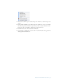
3 Guided Analysis
•
New application wizards:
— Open File
— Display Properties
— Apoptosis
— Cell Cycle - Mitosis
— Co-localization
— Internalization
— Nuclear localization
— Shape change
•
New building blocks to generate graphs with recommended feature choices
and default scaling:
— Single cells
— Focus
— Fluorescence positives
4 Statistics and Reporting
•
New statistic, Concentration. Reports the concentration of a population.
•
View and export statistics for multiple populations or feature values for multiple
objects in the statistics area.
•
New mean and median RD statistics available in the statistics area.
•
View and export graphs in the analysis area with a white (light mode) or dark
(dark mode) background.
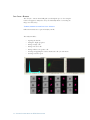
5 Image Display
2 Preface
•
Display settings accommodate 10 and 12 bit imagery as well as higher pixel
intensities that result from EDF deconvolution.
•
Multiple objects in an image are now separated into individual objects.
•
Objects in the image gallery are vertically and horizontally centered.
•
Object numbers appear in the upper left corner of an image and may be turned
off for reporting.
•
Zoom option to enlarge images in the image gallery and in the analysis area.
•
Unlimited columns in Viewing modes in the image gallery.
•
Any mask can be assigned to a column of a viewing mode, regardless of the
image in that column.
6 Compensation
•
Select any .cif, .daf, or .ctm file to obtain a compensation matrix.
•
New compensation menu for viewing and editing compensation matrices and
preview process for testing a matrix.
•
Improved algorithm for selection of positive populations that eliminates saturated events.
7 Feature and Mask Improvements
Features
•
Improved the Object per second and Objects/ml calculations.
•
New Spot Intensity Max feature.
•
New features:
— Ensquared energy
— Raw Centroid X
— Raw Centroid Y
— Shift X
— Shift Y
— XCorr
Masks
•
The Spot mask’s spot to cell background ratio has improved.
•
Inspire mask is new.
Preface 3
4 Preface
Chapter 2
Setting Up the IDEAS® Application
This chapter describes the hardware and software requirements for
the application, which includes the procedures for installing,
removing, and upgrading the application. The following
subsections cover this information:
“Hardware and Software Requirements” on page 5
“Installing the IDEAS® Application” on page 6
“Setting Your Computer to Run the IDEAS® Application” on page 6
“Viewing and Changing the Application Defaults” on page 8
Hardware and Software Requirements
This section states the minimum and the recommended hardware and software
requirements for running the IDEAS application.
Hardware Requirements
The minimum hardware requirements are 512 MB of RAM and a 1-GHz processor.
However, due to the large size of the image files that the ImageStream cell analysis
system creates, a larger amount of RAM will prevent paging and thus increase
performance.
Software Requirements
IDEAS 64 bit version requires that the Windows 7 operating system be installed on
your computer. IDEAS 32 bit version requires Windows SP, Windows 2000 or later
version of the operating system. The latest service pack and any critical updates for the
operating system must be included. You must also install the Microsoft .NET
Framework 2.0, which requires Microsoft Internet Explorer 5.01 or later.
Important: If the software requirements are not met, Setup will not block installation
nor provide any warnings.
Note that service packs and critical updates are available from the Microsoft Security
Web Site.
Setting Up the IDEAS® Application 5
Installing the IDEAS® Application
If the IDEAS application has previously been installed, the previous version will be
removed during installation.
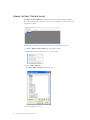
To install IDEAS software
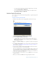
1 Insert the CD or DVD that is labeled IDEAS application. Or download the application Setup file from your account at www.amnis.com.
2 View the contents in My Computer or Windows Explorer.
3 Double-click Setup.exe.
4 Follow the instructions until the installation process has completed.
5 MadCap help viewer is installed and opened during installation or upgrade.
6 An icon appears on the desktop and IDEAS Application appears on the All Programs menu.
Setting Your Computer to Run the IDEAS® Application
“Setting the Screen Resolution” on page 6
“Viewing File Name Extensions” on page 6
“Copying the Example Data Files” on page 7
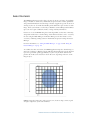
Setting the Screen Resolution
Confirm that the screen resolution is adequate for the IDEAS application. To be able
to view the entire application window, you must set the width of the screen resolution
to a minimum of 1024 pixels.
To set the screen resolution
1 From the Start menu, select Control Panel, and then click Display.
2 Click the Settings tab to set the screen resolution.
Viewing File Name Extensions
When loading a file, the IDEAS application uses the file name extension to determine
the file type. It will be easier for you to distinguish raw image files, compensated image
files, and data analysis files from each other if Windows Explorer does not hide the
extensions.
To view file name extensions
1 In Windows Explorer, go to Tools > Folder Options.
2 Click the View tab, and make sure that the Hide extensions for known file types
check box is not selected.
3 Click OK.
6 Setting Up the IDEAS® Application
Copying the Example Data Files
If the CD or DVD includes data files, copy them to a single directory on your hard
drive. Sample data files are also available on your workstation or at www.amnis.com/
login for customers with an Amnis account.
Note that the default data directory is installation directory\ImageStreamData, where
installation directory is the directory that you installed the IDEAS application in. For
example, the default data directory might be C:\Program
Files\AmnisCorporation\IDEAS\ImageStreamData.
To copy the example data files
1 Copy the data files.
2 Right-click the directory that contains the data files, and click Properties.
3 Clear the Read-only check box.
4 Click OK.
Setting Up the IDEAS® Application 7
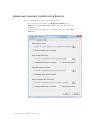
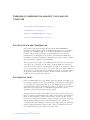
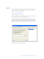
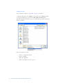
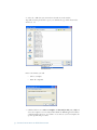
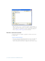
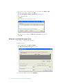
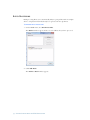
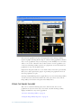
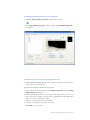
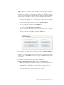
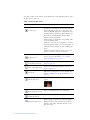
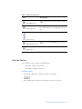
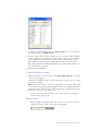
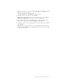
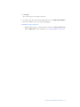
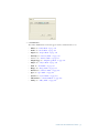
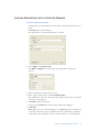
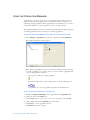
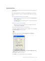
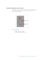
Viewing and Changing the Application Defaults
Files are automatically saved to the specified default directory.
•
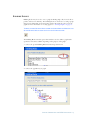
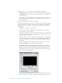
To view or change these defaults, click Application Defaults on the
Options menu, and the Directories tab will be displayed, as shown in the following figure.
•
To view or change the default color or symbol for populations, click the Populations tab.
8 Setting Up the IDEAS® Application
Chapter 3
Overview of the IDEAS® Application
This chapter provides an overview of the IDEAS application user
interface, the files that the IDEAS application creates and uses, the
recommended directory organization and an overview of the
workflow.
“Understanding the Data Analysis Workflow” on page 10
“Overview of compensation, analysis tools and file structure” on
page 12
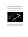
The ImageStream cell analysis system possesses unique capabilities that neither flow
cytometry nor microscopy alone can deliver. Examples include the analysis of
molecule co-localization and translocation, the analysis of cell-to-cell contact regions
and signaling interactions, the detection of rare molecules and cells, and a
comprehensive classification of large numbers of cells. The IDEAS application acquires
data from INSPIRE™, compensates the images, and allows the user to evaluate the
images with data analysis tools.
Overview of the IDEAS® Application 9
Understanding the Data Analysis Workflow
Data analysis in IDEAS begins with opening a raw image file (.rif) that was collected
and saved using INSPIRE on the ImageStream. Then, an existing compensation
matrix or a new compensation matrix is applied to the .rif file and two additional files
are created, the .cif (compensated image file) and .daf (data analysis file).
A compensation matrix performs fluorescence compensation, which removes
fluorescence that leaks into other channels. See “Overview of Compensation” on
page 38 for more information about compensation. A compensated image can
accurately depict the correct amount of fluorescence in each cell image. Compensation
is defined as the correction of the fluorescence crosstalk. When creating the .cif the
IDEAS application also automatically performs corrections to the raw imagery using
values saved from the instrument at the time of data collection. These corrections
include flowspeed normalization, brightfield gains, and spatial registry.
A template is used to define the features, graphs, image display properties and analysis
for the .daf. The default template includes over 200 calculated features per object. An
expanded template is available that includes over 600 calculated features per object.
Within the .daf file, the user can perform many analyses using the tools and wizards
within the application and save the results as a template file (.ast).
The IDEAS application then calculates feature values and shows the data as specified by
the selected template.
Once a data analysis file (.daf file) or compensated image file (.cif file) is saved, it can be
opened directly for data analysis. You would only open a .cif if you wanted to change
the template or a .rif file to change the compensation.
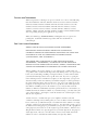
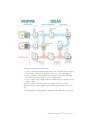
The diagram on the next page displays this workflow.
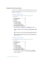
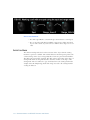
10 Overview of the IDEAS® Application
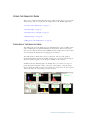
Overview of Data Analysis Workflow
1 Create a compensation matrix using the single color control files. Open an experimental .rif file or from the Compensation menu choose Create New Matrix.
2 A .cif and .daf file are automatically created. Analyze the experimental file using
data analysis tools in the .daf file to create an analysis template.
3 Create a statistics report template within the .daf file and save the data file, and an
anlaysis template.
Note: this is usually done on the positive and negative controls to create the
appropriate analysis and then applied to the rest of the experimental files in the next
step.
4 Perform batch processing, applying compensation and template files created above.
Overview of the IDEAS® Application 11
Overview of compensation, analysis tools and file
structure
“Data Acquisition and Compensation” on page 12
“Data Analysis Tools” on page 12
“Interface of the IDEAS Application” on page 13
“Overview of the Data File Types” on page 13
Data Acquisition and Compensation
Data are first acquired from the ImageStream using the Amnis INSPIRE™
instrument-control application. Next, the IDEAS application processes and analyzes
the image data. The IDEAS application contains the algorithms and tools that are
needed to analyze the imagery. Preprocessing algorithms and tools correct for
instrument biases, including flowspeed variations, spatial alignments, illumination
irregularities, and camera background. Compensation for spectral crosstalk is calculated
from control files and applied to experimental files.
After the preprocessing completes, the IDEAS application allows for the interrogation
of the image data, segmenting out cells, nuclei, cytoplasm, FISH spots, beads, and
other objects of interest. Using a default template, the application calculates the values
for over 200 standard features per object, to be used in subsequent analyses. Guided
analysis for many common applications is available through the use of wizards. Finally,
the application displays imagery and feature-calculation results, and it defines cell
populations in a host of plots and histograms.
Data Analysis Tools
Data in the IDEAS application can be further explored by using the data analysis tools.
For example, populations of cells can be identified by drawing regions on histograms
or scatter plots, or by tagging individual objects. The IDEAS application provides
standard distribution statistics for all defined populations. In addition, users can further
define images by creating features—a mathematical expression that contains
quantitative and positional information about the image.
The application also contains tools that allow you to view grayscale and pseudocolor
images, to apply gains and thresholds, and to build composite images. For individual
images, tools are available to examine pixel intensities, create line profiles of pixel
intensities, and compute the distribution statistics of the pixels in a region of an image.
Both morphological measurements and intensity information are available for
calculating feature values. Histograms and scatter plots display feature data graphically
and the population distribution statistics include a variety of calculations such as the
mean, standard deviation, and coefficient of variation (CV).
12 Overview of the IDEAS® Application
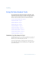
Interface of the IDEAS Application
The IDEAS Application allows the opening of multiple data files within one instance
of the program. Each file is divided into three sections: the Image Gallery, the Statistics
Area, and the Analysis Area. The placement and size of these areas are adjustable.
•
The Image Gallery displays the images of populations of cells, segmentation
masks and composite images . For more information, refer to “Overview of the
Image Gallery” on page 61.
•
The Statistics Area displays feature values for objects and populations in tabular form. For more information, refer to “Overview of the Statistics Area” on
page 89.
•
The Analysis Area displays plots and distributions of cellular feature values.
Individual images and text panels. For more information, refer to “Overview of
the Analysis Area” on page 73.
Overview of the Data File Types
Data from the ImageStream cell analysis system are collected and managed using three
types of data files: raw image file (.rif), compensated image file (.cif), and data analysis
file (.daf).
This section describes each file type and the table summarizes the features of each file.
Overview of the IDEAS® Application 13
Raw Image File (.rif)
The INSPIRE application saves the image data that were acquired by the ImageStream
cell analysis system to a .rif file. A .rif file contains:
•
Pixel intensity data (counts and location) that the camera collected for each
object that the instrument detected
•
Instrument settings that were used for data collection
Compensated Image File (.cif)
The IDEAS application creates a .cif file when the user opens a .rif file and applies a
compensation matrix. The segmentation algorithm automatically defines the
boundaries of each object, creating a mask that is used for calculating feature values.
The applied compensation matrix performs pixel-by-pixel fluorescence compensation
prior to segmentation.
During the creation of the .cif file, the application makes corrections to the imagery.
These corrections include:
•
Removal of artifacts from variability in the flow speed, camera background, and
brightfield gains.
•
Alignment of the objects to subpixel accuracy, which allows the viewing of
multi, composite imagery and the calculation of multi feature values, such as
the Similarity value.
•
Coincident objects are cut apart to place into individual image frames. Note
that this will increase the number of objects in the file.
Multiple .cif files can be created from a single .rif file by applying a different
fluorescence compensation matrix or correction each time a .rif file is opened and
choosing a unique name for the .cif file. Similarly, you can create a new .daf file from a
single .cif file by creating a new name and applying a different analysis template.
Data Analysis File (.daf)
The IDEAS application creates a .daf file while it is loading a .cif file into a template
file (.ast). The .daf file is the interface to visualize and analyze the imagery that the .cif
file contains. The .daf file contains:
•
Feature definitions
•
Population definitions
•
Calculated feature values
•
Image display settings
•
Definitions for graphs and statistics
Loading a .daf file restores the application to the same state it was in when the file was
saved, i.e., with the same views, graphs, and populations. In IDEAS versions 3.0 or
later, a .daf file may be used as a template.
14 Overview of the IDEAS® Application
Note: When a .daf file is opened, the .cif file must be located in the same directory as
the .daf file since the .daf file points to images used for analysis that are stored in the
associated .cif file.
Template (.ast)
The IDEAS application saves the set of instructions for an analysis session in a .daf file
to a template (.ast file). Note that a template contains no data; it simply contains the
structure for the analysis. This structure includes definitions for:
•
Features
•
Graphs
•
Regions
•
Populations
The .ast also contains settings for:
•
Image viewing
•
Image names
•
Statistics
The \templates subdirectory (under the directory where the IDEAS application
was installed) contains the default template, named defaulttemplate.ast. Because a
template is required for loading a .cif file, you must use the default template to create
the first .daf file. After you save a custom template, you can use it for any subsequent
loads of .cif files.
Note: The default template may change between releases of the IDEAS application
software. In IDEAS versions 3.0 or later, a .daf file may be used as a template. The
default template contains over 200 calculated features per object. An expanded
template is also available that includes over 600 calculated features per object.
Compensation Matrix File (.ctm)
The IDEAS application saves the compensation values that are created and saved
during the spectral compensation of control files to a compensation matrix file (.ctm
file). This file has no associated object data; it is created and saved to be applied to
experimental files.
Overview of the IDEAS® Application 15
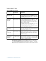
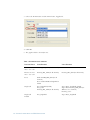
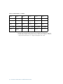
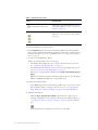
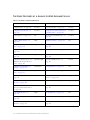
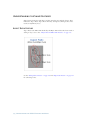
Review of Data File Types
Table 1: Review of Data File Types
File Acronym
and Name
File Creation
Description
.rif
Raw Image File
Created in INSPIRE
Contains instrument setup data, pixel intensity data, and
uncorrected image data from the INSPIRE application.
The IDEAS application uses the .rif file to create a compensated image file (.cif file).
.cif
Compensated
Image File
User creates a .cif
from the .rif and .ctm
Contains imagery that has been corrected for variations in
the camera background, camera gains, flow speed, and
vertical and horizontal positioning between channels.
Serves as a database of images used for feature-value calculations and imagery display.
The IDEAS application also performs fluorescence compensation, if necessary, when creating a .cif file.
The IDEAS application loads the .cif file into a template
to create a data analysis file (.daf file)
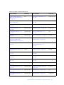
.daf
Data Analysis
File
References the .cif
The main working data file that contains the calculated
feature values, the graphs, and the statistics used for analysis. The .daf file references the .cif.
.ast
Template File
Created from the .daf
This file contains no data; it contains the structure for the
analysis, such as, definitions for features, graphs, regions,
and populations; image viewing settings; image names;
and statistics settings.
.ctm
Compensation
Matrix File
User creates new
.ctm when opening a
.rif
Contains compensation values that are created and saved
during the spectral compensation of control .rif files. This
file has no associated object data; it is created and saved to
be applied to experimental .rif files.
Note about Case Sensitivity: Even though Windows does not treat file names as
case sensitive, the IDEAS application depends on the case-sensitive .rif, .cif, and .daf
file name extensions to identify the file types. Avoid the use of illegal characters for file
names such as: “\/:*?<>!”.
16 Overview of the IDEAS® Application
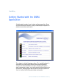
Chapter 4
Getting Started with the IDEAS
Application
Guided analysis makes it easy to start analyzing your data. Once
you are familiar with the basic analysis available you may want to
perform more advanced analysis.
This chapter is divided into two sections. First, guided analysis is
described using the analysis wizards and second, advanced
analysis with more detailed instructions that describe how to
open, compensate, merge, save, and create data files without using
the wizards. Building blocks are also discussed which provide a
short cut method to building commonly used graphs.
Getting Started with the IDEAS Application 17
Guided Analysis
Guided analysis consists of Application Wizards that help you to analyze your data for
specific applications and “Building Blocks:” on page 27 to define specific parameters
for common graphs.
Application Wizards
Application wizards are available to guide you through an analysis. The wizard
window is organized so that the instructions for each step are written at the top of the
window, the progress through the wizard is shown in the list on the right side and
there may be tips provided at the bottom of the window. Follow the instructions in
the wizard to complete an analysis.
The following wizards are available:
General:
•
“Open File:” on page 19
— Guides you through the process of opening a data file
•
“Display Properties:” on page 20 (available only after a file is open)
— Automatically optimizes the display of the pixel intensities
Application specific:
•
“Apoptosis:” on page 21
— Guides you through the process of creating the features and graphs for analyzing apoptosis.
•
“Cell Cycle - Mitosis” on page 22
— Guides you through the process of creating the features and graphs for analyzing the cell cycle and enumerating mitotic events.
•
“Co-localization” on page 23
— Guides you through the process of creating the features and graphs for analyzing the co-localization of 2 probes.
•
“Internalization” on page 24
— Guides you through the process of creating the features and graphs for analyzing the internalization of a probe.
•
“Nuclear Localization” on page 25
— Guides you through the process of creating the features and graphs for analyzing the nuclear localization of a probe.
•
“Shape Change” on page 26
— Guides you through the process of creating the features and graphs for analyzing the circular shape of a cell using a surface stain or brightfield image.
18 Getting Started with the IDEAS Application
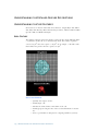
Open File:
This wizard will guide you through the opening of a data file. Use this wizard to open
a file if you are not using one of the application specific wizards. The application
specific wizards incorporate opening a file.
To begin, double-click on Open File
Follow the instructions to open your file.
Tip: You can limit the view to specific file types (.daf, .cif or .rif) by using the dropdown menu ‘Files of type:’ in the Select Data File window.
A .daf file will open directly without further input, a .cif file will require a template
and a .rif file will require a template and a compensation matrix. If the template or
compensation matrix boxes are left blank, the default template and/or matrix will be
applied. For more information on opening data files see “The File Menu” on page 29 .
Once a data file is open you may begin analysis.
Getting Started with the IDEAS Application 19
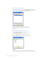
Display Properties:
Once you have an open data file, this wizard is available from the Guided Analysis
menu or from the wizard icon. This wizard will set the image display mapping for the
channel images you select. Brightfield and scatter images will be automatically
adjusted. This wizard is also incorporated into the first steps of the application specific
wizards.
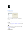
To begin, select wizards from the Guided Analyis menu or click the wizard
icon to the left of the analysis area.
The Wizards window opens.
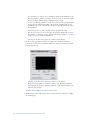
Double-click on the Display Properties option and follow the instructions.
The Display Properties adjusts the mapping of the pixel intensities to the display range
for optimizing the display. This is for display only and does not effect the pixel values.
For more information on image display see “Setting the Image Gallery Properties” on
page 64.
20 Getting Started with the IDEAS Application
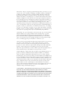
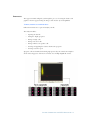
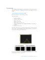
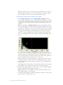
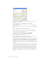
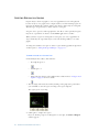
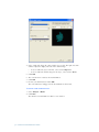
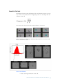
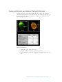
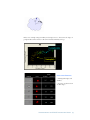
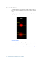
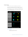
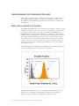
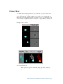
Apoptosis:
The apoptosis wizard will guide you through the process of creating the features and
graphs to measure apoptosis using the images of the nuclear dye and brightfield.
To begin, double-click on Apoptosis
Follow the instructions to open and analyze your file.
The analysis includes:
•
Opening the data file
•
Setting the display properties
•
Gating on single cells
•
Gating on focused cells
•
Gating on fluorescent positive cells
•
Creating and graphing the features that measure apoptosis
•
Creating a statistics report
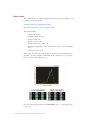
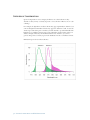
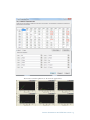
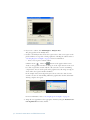
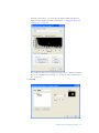
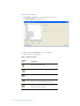
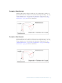
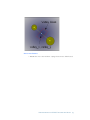
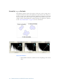
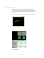
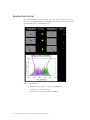
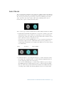
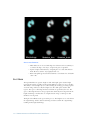
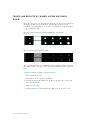
Apoptotic cells are identified in the final graph presented by the wizard. An example is
shown below. Apoptotic cells have low nuclear area and high brightfield contrast.
Getting Started with the IDEAS Application 21
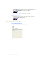
Cell Cycle - Mitosis
The cell cycle - mitosis wizard will guide you through the process of creating the
features and graphs to analyze the cell cycle and identify mitotic events using the
images of a nuclear dye.
To begin, double-click on Cell Cycle - Mitosis
Follow the instructions to open and analyze your file.
The analysis includes:
•
Opening the data file
•
Setting the display properties
•
Gating on single cells
•
Gating on focused cells
•
Gating on fluorescent positive cells
•
Creating and graphing the features that measure cell cycle and mitosis
•
Creating a statistics report
22 Getting Started with the IDEAS Application
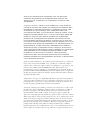
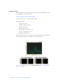
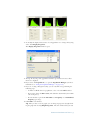
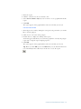
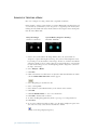
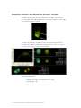
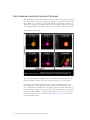
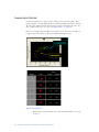
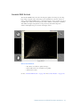
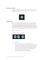
Co-localization
The co-localization wizard will guide you through the process of creating the features
and graphs to measure the co-localization of two probes in any population of cells you
identify.
To begin, double-click on Co-Localization
Follow the instructions to open and analyze your file.
The analysis includes:
•
Opening the data file
•
Setting the display properties
•
Gating on single cells
•
Gating on focused cells
•
Gating on fluorescent positive cells
•
Creating and graphing the feature ‘Bright Detail Similarity’ for measuring colocalization
•
Creating a statistics report
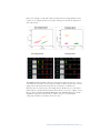
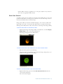
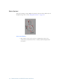
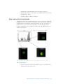
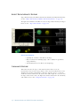
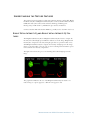
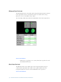
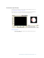
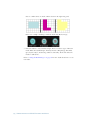
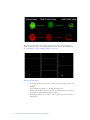
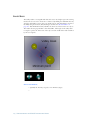
Cells with colocalized probes are identified in the final graph presented in the wizard.
In this example, cells with high Bright Detail Similarity values have co-localization of
the two probes, CD107a (green) and CpG (red).
For a more thorough explanation of the Bright Detail Similarity feature see “Bright
Detail Similarity R3 Feature” on page 184 .
Getting Started with the IDEAS Application 23
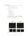
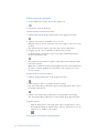
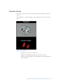
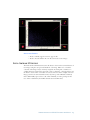
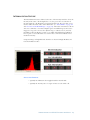
Internalization
This wizard will create an analysis template for measuring the internalization of a probe
in any population of cells you identify.
To begin, double-click on Internalization
Follow the instructions to open and analyze your file.
The analysis includes:
•
Opening the data file
•
Setting the display properties
•
Gating on single cells
•
Gating on focused cells
•
Gating on fluorescent positive cells
•
Creating and graphing the feature
•
Creating a statistics report
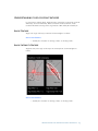
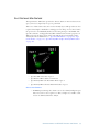
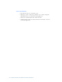
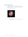
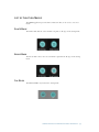
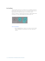
cells with internalized probe are identified in the final graph presented in the wizard.
The example below shows the internalization of labeled CpG (red).
For a more thorough explanation of the Internalization feature see “Internalization
Feature” on page 187
24 Getting Started with the IDEAS Application
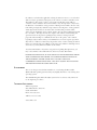
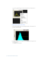
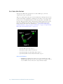
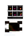
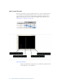
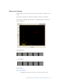
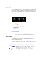
Nuclear Localization
This wizard will create an analysis template for measuring the nuclear localization of a
probe in any population of cells you identify.
To begin, double-click on Nuclear Localization
Follow the instructions to open and analyze your file.
The analysis includes:
•
Opening the data file
•
Setting the display properties
•
Gating on single cells
•
Gating on focused cells
•
Gating on fluorescent positive cells
•
Creating and graphing the feature
•
Creating a statistics report
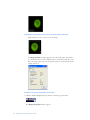
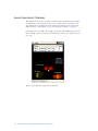
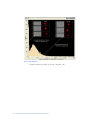
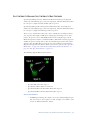
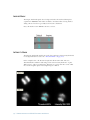
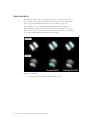
Nuclear localization of a probe is measured using the Similarity feature in the final
graph presented in the wizard. The example shown here is of THP1 cells stimulated
with 1 ug LPS for 90 minutes and stained with DRAQ5 (red) and NFkB (green) to
measure the nuclear localization of the NFkB.
For a more thorough explanation of the Similarity feature see “Similarity Feature” on
page 188 .
Getting Started with the IDEAS Application 25
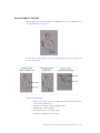
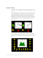
Shape Change
This wizard will create an analysis template for measuring the shape (circularity) of any
population of cells you identify.
To begin, double-click on Shape Change
Follow the instructions to open and analyze your file.
The analysis includes:
•
Opening the data file
•
Setting the display properties
•
Gating on single cells
•
Gating on focused cells
•
Gating on fluorescent positive cells
•
Creating and graphing the feature Circularity of a surface stain or brightfield
image
•
Creating a statistics report
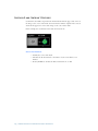
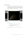
Shape change is measured in the final graph presented in the wizard. Cells with low
circularity scores have a highly variable radius. In this example monocytes in whole
blood were stained with CD14 (green).
For a more thorough explanation of the Circularity feature see “Circularity Feature”
on page 156 .
26 Getting Started with the IDEAS Application
Building Blocks:
Building blocks may be used to create a graph for finding single cells, focused cells or
positive cells based on Intensity. The building blocks are shortcuts to creating a graph
that provide a limited list of relevant features with set X and Y axis scales set for the
graph. For more information on creating graphs see “Creating Graphs” on page 75.
To begin, choose Building Blocks from the Guided Analysis Menu or click
on the Building Blocks icon to the left of the analysis area.
The Building Blocks window opens. This window is used to define a graph with a
specified set of features available depending on the purpose of the graph.
1 Choose the specific Building Block from the drop-down menu.
2 Choose the population(s) to graph.
Getting Started with the IDEAS Application 27
3 Choose the X Axis Feature and the Y Axis feature, if applicable.
4 Click OK.
5 The graph is added to the analysis area.
Table 1: Building blocks overview
Building Block
X axisFeatures
Flourescence Positives - one color
Intensity_MC_ChX (for all channels)
Flourescence Positives - two color
Intensity_MC_ChX (for all channels)
Focus
Gradient RMS_MX_ChX (for all
channels)
Note: Gradient RMS of brightfield is
default
Single Cell
Area_brightfield (default)
Area_scatter
Intensity_MC_ChX (for all channels)
Aspect Ratio_brightfield (default)
Aspect Ratio Intensity_MX_ChX (for
all fluorescence channels)
Intensity_scatter
Single Cell
Default
Area_brightfield
Aspect Ratio_brightfield
28 Getting Started with the IDEAS Application
Y axis Features
Intensity_MC_ChX (for all channels)
Advanced Analysis
“The File Menu” on page 29
“Viewing Sample Information” on page 37
“Overview of Compensation” on page 38
“Creating a New Compensation Matrix File” on page 40
“Merging Raw Image Files” on page 49
“Saving Data Files” on page 51
“Creating Data Files from Populations” on page 52
“Batch Processing” on page 54
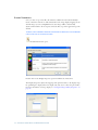
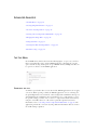
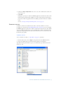
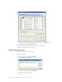
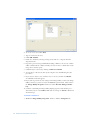
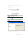
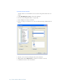
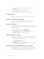
The File Menu
Use the File menu, which is shown in the following figure, to open, save, and close
image and analysis files and to quit the IDEAS application. Alternatively, you may
open a data file by drag and drop into an open IDEAS window. Muliple data files can
be open in one instance of the IDEAS application.
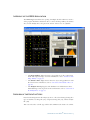
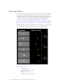
Opening a .rif file
A .rif file is opened when there is new data and the IDEAS application needs to apply
corrections. When opening a .rif file, the IDEAS application corrects each image for
the spatial alignment between channels, camera background normalization, flow speed,
and brightfield gain normalization. If you want fluorescence compensation to correct
for spectral overlap, you must create or choose a compensation matrix at this time by
using the control files that were collected for a particular experiment. For more
information, refer to “Creating a New Compensation Matrix File” on page 40. The
application performs the corrections by using calibration information that was saved to
the .rif file during acquisition.
Getting Started with the IDEAS Application 29
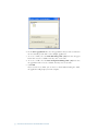
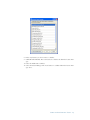
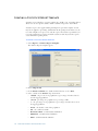
To open a .rif file
To use a wizard to do this see “Open File:” on page 19, otherwise:
1 From the File menu, choose Open or drag the file into the IDEAS window.
2 Select the .rif file that you want in the Select File To Load window.
Tip: while browsing for the file to open you can limit the type of file shown in the
window to .rif files.
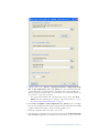
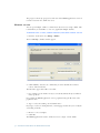
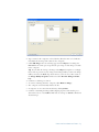
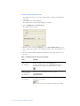
In the next window you will:
•
Choose a compensation matrix
•
Choose a template
•
Name the output files
•
Choose the number of events to process
30 Getting Started with the IDEAS Application
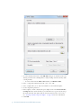
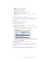
3 Click the folder next to Select a compensation matrix, compensated image
file, or data analysis file (.ctm, .cif, .daf) field to choose the matrix that was
generated from the controls used for the experiment. If you leave it blank, the
default compensation matrix will be used, but this is not recommended unless you
do not want to compensate your data.
•
If a compensation matrix for the experiment has not been made, click New
Matrix. For more information on creating a compensation matrix see “Creating a New Compensation Matrix File” on page 40.
4 In the Select a template or data analysis file (.ast, .daf) field, select a template
file to load by clicking the folder and browsing for the file. If left blank, the Default
template with the basic features, masks, and settings will be used.
5 Name the output files with a new name, if necessary.
6 You may change the number of objects to load in the box under Enter the number of objects to process. The default value is the number of objects in the file.
Getting Started with the IDEAS Application 31
Tip: you can select a smaller number than the maximum if you have a large number
of objects to load. This helps save time for creating a template file. The IDEAS
application randomly loads the specified number of objects within the file.
7 Click OK.
The application then creates the .cif and .daf files and the .daf file is loaded into the
Image Analysis area.
32 Getting Started with the IDEAS Application
.Rif File Option: Setting Advanced Corrections
Most often, the defaults will be adequate. For some older data files, you may need to
provide control files for certain settings.
•
To view the corrections that will be applied to the .rif file, click Advanced
within the Opening a .rif file window.
The Opening file window appears.
•
Make any changes to the corrections that you need, and then click OK. Refer
to the Troubleshooting chapter “Troubleshooting” on page 207 for more
information about these options.
Opening a .cif file
A .cif file is generated when corrections are applied to a .rif file, as described in
“Compensated Image File (.cif)” on page 14. When opening a .cif file, the IDEAS
application calculates feature values and creates a .daf file to display images and graphs.
When opening a .cif file, an analysis template is selected. The template provides the
initial characteristics of the analysis. Opening the .cif file causes the IDEAS application
to calculate feature values and to use populations, graphs, and image viewing settings to
display the cells as defined by the template.
To open a .cif file
To use a wizard to do this see “Open File:” on page 19, otherwise:
1 From the File menu, choose Open or drag the file into the IDEAS window.
Getting Started with the IDEAS Application 33
2 Select the .cif file that you want in the Select File To Load window.
Tip: while browsing for the file to open you can limit the type of file shown in the
window to .cif.
In the next window you will:
•
Choose a template
•
Name the output file
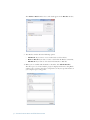
3 Click the folder next to Select a template or data analysis file (.ast, .daf) and
choose the template to use for analysis. If left blank, the IDEAS application will use
a default template. However, it is useful to create and save your own templates for
specific experimental procedures.
34 Getting Started with the IDEAS Application
4 Change the Data analysis file name, if necessary. The default name matches the
name of the .cif.
5 Click OK.
During the opening of a .cif file, the IDEAS application calculates the values of the
features that are defined in the template you selected. The progress is shown by a
progress bar. After the application has successfully opened the .cif file, the .daf file is
saved.
See also: “Saving a Compensated Image File (.cif)” on page 52.
Opening a .daf file
A .daf file contains the calculated feature values so that they will not need to be
recalculated, as described in “Data Analysis File (.daf)” on page 14. To open a .daf file,
the IDEAS application requires the .cif file to reside in the same directory. The .daf file
does not contain any image data, so you can think of the .cif file as the database that
contains the imagery. Because all of the feature values have been saved in it, the .daf
file should open quickly.
To open a .daf file
To use a wizard to do this see “Open File:” on page 19, otherwise:
1 From the File menu, choose Open or drag the file into the IDEAS window.
2 Select the .daf file that you want in the Select File To Load window.
Tip: while browsing for the file to open you can limit the type of file shown in the
window to .daf.
Getting Started with the IDEAS Application 35
The progress is shown by a progress bar. The state of the IDEAS application is restored
to what it was when the .daf file was saved.
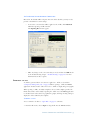
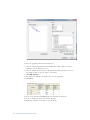
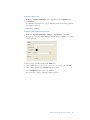
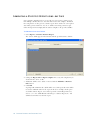
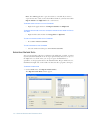
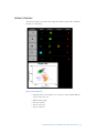
Merging .cif files
You can open multiple .cif files to combine their data and create a single .daf file. This
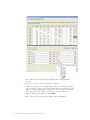
is useful when you would like to create one graph with multiple data files.
To open multiple .cif files, combine their data, and create a single .daf file
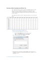
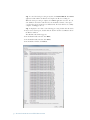
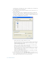
1 From the Tools menu, select Merge .cif Files.
The Load Multiple .cif Files window appears.
2 Click Add Files, and select the .cif files that you want. Click Remove Files to
remove a file from the list.
The file names appear in the Files to Load list.
3 For each file, type the number of objects to load. By default, all objects will load
unless specified.
For each file, the IDEAS application creates a population using the file name as the
population name.
4 Type or select the resulting .cif and .daf file names.
If you type or select an existing file name, a warning appears that asks you to verify the
overwriting of the file.
5 Browse to select a template.
6 Click OK.
The IDEAS application loads the .cif files and creates a single .cif and .daf file.
36 Getting Started with the IDEAS Application
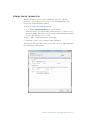
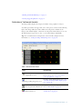
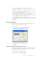
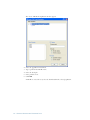
Viewing Sample Information
All of the information associated with an IDEAS file, such as the collection
information, camera settings and corrections, is saved within IDEAS and can be
viewed in the Sample Information window.
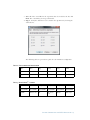
To open the Sample Information window
1 Go to Tools > Sample Information to open the window.
Information for the open data file will be loaded otherwise you can browse for a
data file by clicking on the folder. You can open the Sample Information Window
for any of three file types: .rif, .cif, or .daf.
2 Select a Tab to see the information for each heading.
3 Click Print to print a report of all of the sample information.
Tip: You may click on the folder and browse for a file to view the sample information
for any file without loading the file.
Getting Started with the IDEAS Application 37
Overview of Compensation
Spectral compensation corrects imagery for fluorescence that leaks into nearby
channels so that you may accurately depict the correct amount of fluorescence in each
cell image.
For example, the light from one fluorochrome may appear primarily in channel 3, but
some of the light from this fluorochrome may appear in channel 4 as well, because the
emission spectrum of the probe extends beyond the channel 3 spectral bandwidth. The
light from a second fluorochrome may appear primarily in channel 4 but, unless you
subtract the light emitted by the first fluorochrome into channel 4, you cannot
generate images that accurately represent the distribution of the second fluorochrome.
Emmission Spectra for two fluorochromes:
38 Getting Started with the IDEAS Application
Below is an example of cells stained with two fluorochromes independently and run
together as one sample. Intensity scatter plots and images are shown uncompensated
and compensated.
Uncompensated
Compensated
The IDEAS application builds a matrix of compensation values by using one or more
control files. A control file contains cells stained with one fluorochrome. You can mix
singly stained cells and run them together, but you must be careful that the
fluorochromes do not bleed onto other singly stained cells. Because it is critical that
matrix values be calculated from intensities derived from a sole source of light, control
files are collected without brightfield illumination. The IDEAS application performs
brightfield compensation when it loads a .rif file. The process of creating the
compensation matrix is described in the next section.
Getting Started with the IDEAS Application 39
Creating a New Compensation Matrix File
The compensation matrix is a table of coefficients. The IDEAS application uses this
table to place the detected light that is displayed in each image into the proper
channels, on a pixel-by-pixel basis. The coefficients are normalized to 1. Each
coefficient represents the normalized amount of the leakage of the fluorochrome into
the other channels.
The default matrix, which is used if no compensation matrix is chosen, is the identity
matrix.
To generate a new compensation Matrix file
1 Start the Compensation Wizard in one of two ways:
— Click the New Matrix button when opening a .rif file
— OR select Compensation>Create New Matrix .
The compensation wizard opens to Step 1:
2 Add compensation control files by clicking Add Files and browsing for the no
brightfield control files for the experiment. Hold down the control key to select
multiple files at once.
40 Getting Started with the IDEAS Application
3 When all of the control files for the experiment have been added to the list, click
Next. The control file(s) are merged and loaded.
4 Step 2: Verify the channels for each control in the experiment by checking the
channel boxes.
The following tables are provided as a guide for each instrument configuration.
Table 2: First generation ImageStream
Ch 1
Ch 2
Ch3
Ch 4
Ch 5
Ch 6
470-500nm
400-470nm
500-560nm
560-595nm
595-660nm
660-735nm
Scatter
DAPI
Fluorescein
PE
7-AAD
PE-Cy5
Table 3: ImageStreamX- 1 camera
Ch 1
Ch 2
Ch 3
Ch 4
Ch 5
Ch 6
430-505nm
505-560nm
560-595nm
595-660nm
660-745nm
745-800nm
DAPI
Fluorescein
PE
PE-TexasRed
AF647
APC-Cy7
Getting Started with the IDEAS Application 41
Table 4: ImageStreamX- 2 camera
Ch 1
Ch 2
Ch 3
Ch 4
Ch 5
Ch 6
430-480nm
480-560nm
560-595nm
595-660nm
660-745nm
745-800nm
BF
Fluorescein
PE
PE-TexasRed
PE-Cy5
PE-Cy7
Ch 7
Ch 8
Ch 9
Ch 10
Ch 11
Ch 12
430-505nm
505-570nm
570-595nm
595-660nm
660-745nm
745-800nm
DAPI
Pacific
Orange
BF
Texas Red
AF647
APC-Cy7
5 Background and spatial offset corrections are performed, the imagery is displayed,
bivariate plots of adjacent channels Intensity are added to the analysis area and the
compensation matrix values are computed and displayed in a table.
42 Getting Started with the IDEAS Application
The Positive Control Populations are shown in the graphs below.
Getting Started with the IDEAS Application 43
6 In Step 3, choose one of two methods for calculating the coefficients.
•
The Best Fit method is used for objects such as cells where intensities vary.
•
The Means method is used for objects such as beads that have only slight variations in intensity.
•
For each fluorochrome, the application automatically identifies a positive control population, excluding the brightest and dimmest objects, and assigns it to
the proper channel.
7 Inspect the matrix values in the table of coefficients.
Coefficients should always be less than 1, and decrease from the assigned channel.
In other words, leakage should be greater in the channel nearest to the assigned
channel. Fluorescence always extends in the long-wavelength direction from the
exciting light.
•
Verify that no coefficients are larger than 1.
•
Verify that, in a column corresponding to a fluorochrome, the coefficients
decrease from the assigned channel.
•
Verify that the coefficient is greater in the channel below the 1 in the table than
the value above the 1 in the table. Verify that these coefficients also decrease in
subsequent channels below the 1.
•
Verify that there are no changes from the identity matrix in the columns where
there are no fluorochromes, including the scatter and brightfield channels. If
necessary, the column can be set to the identity values by double-clicking on
the heading.
•
Inspect the coefficients in the matrix by double-clicking on the coefficient.
Coefficients highlighted by red have errors greater than 1%.
A graph representing the coefficient appears. The population potted in the
graph is the positive control population of the column of the coefficient. The
X Axis represents the intensity in the assigned channel of the fluorochrome.
The Y Axis represents the intensity in the channel of leakage. The coefficent
value and error are also displayed.
•
You can use the automatically generated control populations as they are, or you
can refine them and create different populations by using the region tools. See
44 Getting Started with the IDEAS Application
the option below to remove objects from the population. By default, the populations are named 3_Positive, 5_Positive, and so on. You can view the populations in the Image Gallery. Some populations may be empty.
•
To choose a different population, use the arrow and select the population from
the list. The hierarchical relationship is shown in the population list. Assign
populations only to the channels that correspond to the fluorochromes used in
the experiment.
•
If you want to clear a column, double click on the channel heading.
•
If needed, you can create new scatter plots by using the Analysis Area toolbar.
For example, a 4_Intensity versus 5_Intensity plot may be useful. See “Creating
Graphs” on page 75 for more information.
The slope of the line on the plot is the coefficient in the matrix.
8 If objects in the population exist that are outliers, they should most likely be
removed from the positive population within the compensation matrix by the following optional steps.
The slope of the line on the plot is the coefficient in the matrix.
If objects in the population exist that are outliers, they should most likely be
removed from the positive population within the compensation matrix by the
following optional steps.
Option: Remove Objects from the Population
1 Within Step 2 of the compensation wizard, double-click the coefficient to display
the intensity plot.
45 Getting Started with the IDEAS Application
2 If you notice outliers, click Add Graph to Analysis Area.
The plot populates in the Analysis Area.
3 Return to the Analysis Area and use the region tools to draw a new region on the
plot that defines a new positive control population, excluding the outliers. Refer to
“Creating Regions on Graphs” on page 80 for more information.
•
Create a new region to exclude outliers.
Click the Resize
and Zoom
buttons on the graph toolbar to more
clearly see the population of interest. Using one of the region buttons on the toolbar, draw a region that contains only the cells you want to use for determining
compensation. You can click a point on the graph and view the image to help you
decide where the region boundaries should be.
In the example below, the Polygon Region tool was selected to draw a border
around a selection of cells. Clicking within the graph anchors the line and doubleclicking completes the region.
For more information, refer to “Creating Regions on Graphs” on page 80.
4 Assign the new population to the appropriate channel by using the Positive Control Populations list for that channel.
46 Getting Started with the IDEAS Application
5 The coefficient value is automatically recalculated when a new population is
selelcted.
6 Repeat these steps as required to redefine the coefficients.
7 Click Preview Images to view individual objects with corrections applied. Double
click on an image to add it to the preview window. Note: the corrections are only
applied to on-camera channels. For example, if the object is brightest in channel 3
on the first camera, only channels 1-6 are shown corrected for that object.
8 When the matrix appears satisfactory, click Finish.
9 Enter a name for the compensation matrix file (.ctm) and click Save
47 Getting Started with the IDEAS Application
.
Note: The matrix is saved as a compensation matrix file (.ctm file). This file contains the compensation values and can be opened later for editing. To provide the
values for fluorescence compensation, you select a .ctm file when opening a .rif
file. See “Opening a .rif file” on page 29 for more information.
Preview a compensation matrix
A compensation matrix can be applied to a population or .rif file in a preview mode
for editing a matrix.
To open a compensation Matrix
1 Select Open>Compensation Matrix from the File menu or Select View/Edit compensation matrix from the Compensation menu to view, edit or preview the
matrix on image data.The matrix values are displayed in a table and may be edited.
48 Getting Started with the IDEAS Application
2 To preview the matrix on image data, browse for a file or select a population from
the current file to preview and click Preview.
3 You may repeat editing the matrix and previewing until satisified.
4 When done, click OK and save the matrix.
Merging Raw Image Files
You can merge .rif files together for analysis.
To merge .rif files
1 On the Tools menu, click Merge .rif Files.
The Merge Raw Image Files window appears.
2 To select the .rif files to merge, click Add Files.
The .rif file names appear in the list.
49 Getting Started with the IDEAS Application
3 If you want to remove a file from the list, select it and then click Remove File.
4 When the merge list is complete, click OK.
The Save Merged Raw Image (.rif) File dialog box appears.
5 Type a unique file name.
6 Click Save.
The Creating merged .rif file window appears.
When the merge is complete, the Merged .rif Created message appears.
7 Click OK.
Merging Compensated Image Files
You can merge .cif files together for analysis.
To merge .cif files
1 On the Tools menu, click Merge .rif Files.
The Merge Raw Image Files window appears.
2 To select the .cif files to merge, click Add Files.
50 Getting Started with the IDEAS Application
The .cif file names appear in the list.
3 If you want to remove a file from the list, select it and then click Remove File.
4 Type a unique name for the output files.
5 Select a template..
6 Click OK.
7 The merged files are created and the new .daf file is loaded with a population created from each file.
Saving Data Files
Data files are saved at several stages of analysis. Raw image files are saved during data
acquisition, by merging multiple .rif files or by creating new files from populations.
Compensated image files and Data analysis files are saved when opening .rif files,
opening multiple .cif files, using the file menu or when running a batch analysis. The
IDEAS application also saves other types of files that are used for data correction and
presentation. Template files (.ast) save the structure of an analysis and compensation
matrix files (.ctm) save the compensation matrices.
Application Defaults are set that direct the files into specific folders and can be viewed
or changed by the user. See “Viewing and Changing the Application Defaults” on
page 8 for more information.
Saving a Data Analysis File (.daf)
A .daf file contains a snapshot of an analysis as described in “Data Analysis File (.daf)”
on page 14. Saving the analysis as a .daf file allows you to recall that analysis simply by
opening the file. When you quit the IDEAS application, you are always prompted to
save changes to a .daf file. You can also save changes from the File menu. Remember
that the .daf file does not contain image information, so opening the .daf file requires
the related .cif file to reside in the same directory.
To save a .daf file
1 On the File menu, click Save as Data Analysis File (.daf).
2 Enter a file name. Note that the default directory is the one where the .cif file was
saved.
If you select an existing file name, a warning appears that asks you to verify the
overwriting of the existing file.
3 Click Save.
The data is now ready for analysis. You can create graphs, view imagery, and display feature values and statistics. After you have defined an analytical procedure in
the .daf file, you can save the file as a template, which allows you to use the procedure for analyzing other files. Refer to “Using the Data Analysis Tools” on page 59
for more information.
option: Saving a data analysis file with only the feature values used.
When you want to reduce the size of a data analysis file you may save the .daf with
only the features that are used for analysis of statitics or graphs.
51 Getting Started with the IDEAS Application
On the File menu, click Save as Data Analysis File - Used Features Only. and follow
the instructions 2-3 above.
Saving a Compensated Image File (.cif)
The IDEAS application creates and saves a .cif file when a .rif file is opened. By
default, the application names the .cif file with the same name that the .rif file has,
replacing the .rif extension with .cif. The application also places the .cif file in the same
directory as the .rif file. The .cif file will be larger than the .rif file because the .cif file
contains masking information as well as corrected and/or compensated images.
Saving a Template (.ast)
Saving an analysis as a template allows you to apply the structure of the analysis to
other .cif files. Save a template file after saving a .daf file. A template includes all graph
definitions, Image Gallery settings, feature definitions, and statistics settings. No data
are saved in a template. Therefore, selected images and populations that are dependent
on specific objects, such as tagged populations, are not saved.
To save a template
1 On the File menu, click Save As Template File (.ast).
A Save File dialog box appears.
2 Enter the name of the file to save.
3 Click Save.
If you select an existing file name, a warning appears that asks you to verify the
overwriting of the existing file.
Tip: You can change the default template directory in the menu Analysis >
Application Defaults.
Creating Data Files from Populations
To further analyze a population or merge it with other data when working in a .daf,
you can save it to a new data file. This course of action is useful if your data file
contains a large number of objects that are not pertinent to your experiment.
Decreasing the data file size results in better performance by the IDEAS application, as
described in “Creating Regions on Graphs” on page 80. Note that you cannot create a
new .cif or .rif when multiple data files are open.
To create data files from populations
1 On the Tools menu, click Create Data File from Populations.
The Create .cif and/or .rif From Populations window appears.
52 Getting Started with the IDEAS Application
2 In the Select populations list, select the populations that you want to include in
the new data file(s). Ctrl click to select multiple populations.
3 To create a .rif file, select the New Raw Image File (.rif) check box, the population name is used as a default. You may enter a new name.
4 To create a .cif file, select the New Compensated Image File (.cif) check box,
the population name is used as a default. You may enter a new name.
5 Click OK.
If you created a new .cif file, you can choose to load it. When loading the .cif file,
the application will prompt you for the template.
53 Getting Started with the IDEAS Application
Batch Processing
Batch processing allows you to automatically analyze a group of files with one template
when a compensation matrix has already been generated for the experiment.
To perform batch processing
1 On the Tools menu, select Batch Data Files.
The Batches window appears. It lists a record of all batches you have processed.
2 Click Add Batch.
The Define a Batch window appears.
54 Getting Started with the IDEAS Application
3 To select the files for the batch, click Add Files. Navigate to the files and select by
clicking on the file. Select multiple files to add by holding down the Ctrl key while
selecting the files.
•
To remove files from the Files to Process list, click Remove Files.
4 Select a compensation matrix from a file (.ctm, .cif, or .daf).
5 Select a template file (.ast or .daf). Leave blank to use the Default template.
6 Set the output files parameters.
7 If the template contains a Statistics Report template click on the Preview Statistics Report button. Order the files as you wish them to be reported by selecting a
file with a left-click, then right-click the desired position and select ‘move here’.
See “Creating a Statistics Report Template” on page 116 for more information.
8 Click OK.
55 Getting Started with the IDEAS Application
The Define a Batch window closes. The batch appears in the Batches window.
9 The Batches window offers the following options:
•
Add Batch: If you want to create another batch to add to the list.
•
Remove Batch: If you want to remove a batch from the Batches to Run list.
•
Edit Batch: If you want to edit a batch in the Batches to Run list.
10 When you are satisfied with the Batches to Run list, click Submit Batches.
The files to process are listed and the progress is displayed in the Processing Batch
window. Once you have started processing batches, it may use up a fair amount of
your computer’s processing power.
56 Getting Started with the IDEAS Application
Tip: To cancel the batch processing at any time, click Cancel Batch. The IDEAS
application will confirm cancellation and complete the file it is working on.
When the batch processing is complete, the IDEAS application saves the .rif, .cif,
and .daf files in the batch results directory. In the Batches window, a list of processed batches appears in the Processed Batches list. If a batch did not successfully
complete, it will appear in red.
Tip: To display the error that occurred during processing, double-click the batch.
11 If you want a batch report, double-click the batch in the Processed Batches list of
the Batches window.
The Batch Results window appears.
12 In the Batch Results window, click Print.
13 In the Batch Results window, click Close.
14 In the Batches window, click Close.
57 Getting Started with the IDEAS Application
58 Getting Started with the IDEAS Application
Chapter 5
Using the Data Analysis Tools
This section describes how to view imagery; graph data; create
populations by drawing regions in graphs, or by tagging objects;
perform statistical analysis of data; and create new features.
“Overview of the Data Analysis Tools” on page 59
“Using the Image Gallery” on page 60
“Using the Analysis Area” on page 73
“Using the Statistics Area” on page 89
“Using the Mask Manager” on page 94
“Using the Feature Manager” on page 101
“Using the Population Manager” on page 108
“Using the Population Manager” on page 108
“Using the Region Manager” on page 111
Overview of the Data Analysis Tools
The IDEAS application provides a powerful tool set that allows you to explore and
analyze data. The rich feature set lets you create hundreds of your own features to
differentiate objects and statistically quantify your results.
As shown in the following figure, the application window is divided into three
panels—Image Gallery, Statistics Area, and Analysis Area—which each provide the
corresponding tools that you can use for data analysis. There are muliple window
layouts with resizable panels.
Using the Data Analysis Tools 59
You can create populations of objects by tagging hand-selected images, drawing
regions on graphs, and using Boolean logic to combine existing populations. Another
way to create a population of objects is by basing it on the similarity of a set of feature
values to one or more cells in the data set. After you have created a population, you
can view it in the Image Gallery or plot it on a graph. You can view the statistics for
populations or objects in the Statistics Area.
Graphs show data plotted with one or two feature values, and tools are provided that
allow you to draw regions for the purpose of generating new populations. You can
show any population on a plot.
Selecting an individual data point in a graph allows you to view it in the Image Gallery
or look at its feature values in the Statistics Area. Any object that is selected in the
Image Gallery is also shown on the plots in the Analysis Area.
Using the Image Gallery
This section contains the following subsections, which describe how to view
populations of objects in various ways, view masks, customize the Image Gallery
display, and hand-select objects for a population:
“Overview of the Image Gallery” on page 61
“Setting the Image Gallery Properties” on page 64
60 Using the Data Analysis Tools
“Working with Individual Images” on page 70
“Creating Tagged Populations” on page 71
Overview of the Image Gallery
The Image Gallery displays the imagery and masks of any population of objects.
A toolbar is provided in the upper-left corner of the panel, as shown in the following
figure. The Image Gallery also makes different viewing modes available for the
imagery. The default template contains the viewing modes which allows you to view
all channel images in grayscale or color, or each channel image individually.
Tip: You can build custom viewing modes as shown in this example. For more
information, see “Setting the Image Gallery Properties” on page 64.
Table 1: Image Gallery Tools
Tool
Description
Tagging Mode Tool
Allows you to create a population of handpicked objects. See: “To create a handselected population” on page 71.
Image Gallery Properties Tool
Provides custom display features. See: “To
customize the Image Gallery display properties” on page 65.
Show Segmentation Mask Tool
Displays masks on the imagery. See: “To
show or hide masks” on page 62.
Show Color Tool
Sets the Image Gallery color. See: “To show
or hide color” on page 63.
Using the Data Analysis Tools 61
Table 1: Image Gallery Tools
Tool
Description
Show Saturation Color Tool
Zoom Tools
Click on the tool and it will show any saturated pixels will turn red. See: “To show saturation” on page 63.
Zoom in or out and reset zoom on the image
gallery. See: “To zoom on the image gallery”
on page 63
To view the imagery for a population
1 In the Population drop down menu of the Image Gallery, click the population
that you want. (The list includes all the populations as well as the currently selected
bin from a histogram.) To create a population, refer to “Creating Tagged Populations” on page 71.
2 To select an individual image, click it.
A thin, green frame indicates the selected object.
•
The Statistics Area displays the object’s feature values if an object is selected.
See “Overview of the Statistics Area” on page 89.
•
The Analysis Area identifies the object in each scatter plot graph with a green
cross. See “Overview of the Analysis Area” on page 73.
•
The image can be placed in the Analysis area by right click>Display Single
Image.
Tip: Conversely in the analysis area, clicking a graphical point causes the Image
Gallery to highlight and display the corresponding object.
To change the viewing mode
•
In the View drop down menu of the Image Gallery, select a specific view. The
imagery display changes according to the new view. See “To customize the
Image Gallery views images and masks” on page 67 for more information.
To show or hide masks
•
Click the Show Segmentation Masks toolbar button to toggle between
showing and hiding the selected masks for all images in the Image Gallery. See
“To change the name or color for each image” on page 65 for more information.
The mask is shown as a transparent cyan layer over each image.
62 Using the Data Analysis Tools
Tip: To hide the mask for a specific channel only, set the individual channel
mask to None. For more information, see “Setting the Image Gallery Properties” on page 64.
To show or hide color
•
Click the Show Color toolbar button to toggle between showing and hiding
the colors for all images in the Image Gallery. See “To change the name or
color for each image” on page 65 for more information.
To zoom on the image gallery
•
Click the Zoom In toolbar button to view the images in the gallery closer and
the Zoom Out or Reset Zoom to reverse the zoom.
To show saturation
•
Click the Show Saturation Color toolbar button.
Saturated pixels in images, if any, appear in red.
Using the Data Analysis Tools 63
Setting the Image Gallery Properties
When a new data file opens in the default template, you might find it difficult to
clearly see cell morphology because the Image Gallery display properties have not yet
been properly adjusted for the data set.
To optimize the display you may use the wizard “Display Properties:” on page 20 to
set the pixel intensity mapping to the display range. Manual adjustment is described
below.
Clicking the Image Gallery Properties toolbar button opens the Image Gallery
Properties window, which contains the following tabs:
•
Display Properties—Allows you to define the name, color, and display intensity mapping for each image. Allows adjustment of the image size for the image
gallery.
•
Views—Allows you to customize the views for the Image Gallery.
•
Composites—Allows you to create composites and adjust the amount of color
from a channel that is included in a composite image.
64 Using the Data Analysis Tools
To customize the Image Gallery display properties
1 Click the Image Gallery Properties toolbar button to begin.
The Image Gallery Properties window appears with the Display Properties
tab displayed.
To change the size of the panels in the image gallery
1 Display Width and Display Height can be specified or changed to Auto Fit in the
lower left section of this window.
To change the name or color for each image
1 Select an image in the list of images on the Display Properties tab of the Image
Gallery Properties window.
2 On the right side of the window you can type a new, unique name for the selected
image. Note that each image is provided with a default name and the image names
appear near the top of the Image Gallery.
3 Click the colored square for the selected image.
4 Click the color that you want in the color palette.
5 Click OK to close the palette.
Using the Data Analysis Tools 65
Tip: The grayscale image in each channel is assigned a default color for image display in the gallery. Setting the color to white is equivalent to using the original
grayscale image. The colors are also used to build composite images.
To fine-tune the image display intensity for an image
1 On the Display Properties tab of the Image Gallery Properties window,
select an image by clicking the image name in the list. The graph for the currently
selected image is shown in the window and updates as the changes are made. Select
and image in the image gallery that has intensities for the image channel you are
adjusting.
Note: You will adjust the Display Intensity settings on the graph (the Y Axis),
the value of the display to (the X axis), the range of pixel intensities. The range of
pixel intensities will depend on the instrument and the collection mode set during
acquisition. The display range is 0–255; the range of intensities from the camera is
0–1023 (10 bits) for the first generation ImageStream or 0-4095 for the ImageStreamX or 0-32,767 for EDF mode collection. The limits of the graph enable
you to use the full dynamic range of the display to map the pixel intensities of the
image.
At each intensity on the X Axis of the graph, the gray histogram shows the number
of pixels in the image. This histogram provides you with a general sense of the
range of pixel intensities in the image. The dotted green line maps the pixel intensities to the display intensities, which are in the 0–255 range.
Manual setting is done by Click-dragging the vertical green line on the left side
(crossing the X Axis at 0) allows you to set the display pixel intensity to 0 for all
intensities that appear to the left of that line. Doing so removes background noise
from the image.
Click-dragging the vertical green line on the right side allows you to set the display
pixel intensity to 255 for all intensities that appear to the right of that line.
2 From the Image Gallery window, select the object to use for setting the mapping.
It appears in the Image Gallery Properties window.
Tip: You might need to select different objects for different channels because an
object might not fluoresce in all channels.
3 To adjust the pixel mapping for display, click-drag the vertical green line by clicking near it (but not near the yellow cross).
66 Using the Data Analysis Tools
Tip: For fluorescence channels, set the vertical green line that appears on the left
side to the dimmest pixel in the image and set the right vertical green line to the
brightest pixel. To get a good mapping range, adjust the same line so that the yellow cross is centered among the pixel intensities on the X Axis. For the brightfield
channel, set the vertical lines to about 50 counts to the right and left of the histogram to produce an image with crisp brightfield contrast.
•
To change the mapping curve to be logarithmic or exponential, click-drag the
yellow cross.
•
To restore the mapping to a linear curve, Click Set Linear Curve.
•
To see the full scale for the X Axis Click Full Scale.
•
To set the display mapping of the X Axis to the lowest and highest values for a
selected object, Click Set Range to Pixel Data.
•
To set the scale of the X Axis to the range of the vertical green lines or of all the
pixel intensities for the selected object—whichever is larger—Click Autoscale.
•
You may enter values manually by selecting the Manual tab.
4 If you want to preview the changes in the Image Gallery, click Preview Changes
in Gallery.
5 Continue customizing the Image Gallery display properties with another procedure
in this section, or click OK to finish and save changes or Cancel to finish and discard changes.
To customize the Image Gallery views images and masks
1 Within the Image Gallery Properties window, click the Views tab.
Note: The Image Gallery view can be customized to view any combination of
channel images or composites. The default view All Channels is a view that
displays all image channels that were included during acquisition of the file
with their associated default masks. This mask may be changed for the default
view however, the images in this view cannot be changed.
Using the Data Analysis Tools 67
2 To create a new view, Click New.
3 Type in a name for the view.
4 Click Add Column.
5 Define the column by selecting an image and a mask or a composite from the
dropdown menu.
6 Repeat the previous 2 steps until finished adding columns to the view. A column
will be added under the column currently selected. To insert a column click on the
image above insertion point.
7 Columns may be removed by clicking on Remove Column.
8 A view may be edited at any time by selecting the view and following the same
procedures.
9 If you want to delete a view, click the view to select it, and then click Delete.
A confirmation window appears.
10 If you want to preview any new changes in the Image Gallery, return to the Image
Gallery and choose your new view in the View drop down menu. Then return to
the Image Gallery Properties window and click Preview Changes in Gallery.
11 Continue customizing the Image Gallery display properties with another procedure in this section, or click OK to finish and save changes or Cancel to finish and
discard changes.
To create a composite
1 Within the Image Gallery Properties window, click the Composites tab.
68 Using the Data Analysis Tools
2 Type a name for the composite or leave blank to allow the name to be built automatically from the image names added to the composite.
3 Click Add Image. The selected image appears in the Object box. Change the
Percent if desired. The percent specifies the percentage of of the image to include
in the composite.
Tip: As you make the changes, the image in the Object box updates accordingly.
If you want to preview any new changes in the Image Gallery, return to the Image
Gallery and select the View drop down menu to your new view. Then return to
the Image Gallery Properties window and click Preview Changes in Gallery.
4 Continue to add images as desired.
5 To remove and image from the composite, Click Remove Image.
6 The composite is automatically added to the list .
7 A composite can be removed from the list by clicking Delete.
8 Continue customizing the Image Gallery display properties with another procedure in this section, or click OK to finish and save changes or Cancel to finish and
discard changes.
Using the Data Analysis Tools 69
Working with Individual Images
You can work with individual images in the Image Gallery. You can zoom in or out
on the images. You can add a larger version of an image to the Analysis Area for further
analysis, show or hide masks for a single image in the Image Gallery, and copy one or
more images to the Clipboard.
To manipulate individual images
1 In the Image Gallery, right-click an image that you are interested in.
A menu appears.
•
To place the image in the Analysis Area, click Display Single Image. (For
more information, see “Analyzing Images” on page 85.)
•
To show or hide the masks for the object image, click Show Masks or Hide
Masks, respectively. (One or the other will appear depending on the current
state.)
•
To turn the colors on or off for the object image, click Color On or Color
Off, respectively.(One or the other will appear depending on the current state.)
•
To show or hide the saturation color for the object image, click Show or
Hide Saturation Color respectively.(One or the other will appear depending
on the current state.)
To copy images for use in reports
1 In the Image Gallery, right-click an image that you are interested in.
A menu appears.
•
To copy the image to the Clipboard, click Copy Image to Clipboard.
•
To copy the single channel image to the Clipboard, click Copy Column
Image to Clipboard.
70 Using the Data Analysis Tools
•
To copy the single channel image for all of the displayed images to the Clipboard, click Copy Column to Clipboard.
•
To copy all the visible images in the Image Gallery to the Clipboard, click
Copy Displayed Images to Clipboard.
Creating Tagged Populations
You can hand-select objects from either the Image Gallery or a graph and group them
into a population.
To create a hand-selected population
1 Within the Image Gallery, click the Tagging Mode toolbar button to begin.
The Tagged Populations window appears.
2 Select either Update existing or Create New.
•
To Create New, double-click images within the Image Gallery and select
Save. Create a new population name and display properties in the Create a
New Population window.
3 If you selected Update existing, choose a population to update in the drop down
menu.
4 In the Image viewing mode list, choose the mode that you want from the drop
down menu. See “To customize the Image Gallery views images and masks” on
page 67 for more information.
5 To add or remove an image from the tagged population, double-click either the
image in the Image Gallery or a dot in a bivariate plot.
The selected channel image for each tagged cell is displayed in the viewing area of
the Tagged Populations window. In the Image Gallery, a small smiley-face icon
appears on the left side of each tagged image. Each tagged object is also displayed as
a yellow star in a graph in the Analysis Area.
6 If you are updating an existing population, click the Update button in the Tagged
Populations window.
7 When you are finished, click Close in the Tagged Populations window.
Using the Data Analysis Tools 71
Note: The tagging mode remains open until you click Close, and as long as the
Image Gallery is in tagging mode, you cannot create, resize, or move any regions
on the graphs.
72 Using the Data Analysis Tools
Using the Analysis Area
This section contains the following subsections, which describe how to create graphs,
analyze images, and use text panels in the Analysis Area of the IDEAS application:
“Overview of the Analysis Area” on page 73
“Creating Graphs” on page 75
“Creating Regions on Graphs” on page 80
“Analyzing Images” on page 85
“Adding Text to the Analysis Area” on page 88
Overview of the Analysis Area
The Analysis Area provides display space for individual images, plots of cellular feature
values, visualizations of population distributions and statistics, and text annotations.
You can select different layouts for the IDEAS window and placement of the analysis
area and expand the Analysis Area by dragging it’s boundaries.
The Analysis Area is divided into panels of a fixed size. The size of the panels is
automatically adjusted to fit in the available display space. A vertical scroll bar appears
when the number of panels exceeds the space available on the window.
As illustrated by the following figure, the Analysis Area can contain seven types of
panels: histogram, histogram overlay, scatter plot, channel image, composite image,
and text. Each panel will contain its own toolbar and context menu. To move a panel
click on the bar at the top and drag to another location.
Using the Data Analysis Tools 73
A toolbar is visible on the left side of the Analysis Area. The following table describes
the function for each tool..
Table 2: Analysis Area Tools
Tool
Description
Pointer Tool
Provides the normal mode of interaction with the
graphs. Clicking a point on a scatter-plot graph
causes the IDEAS application to display the corresponding image in the Image Gallery (if the population that is currently displayed in the Image
Gallery contains that point).
Click an image to display the corresponding statistics in the Statistics Area.
Click the top of a bin in a histogram to select the
bin. In the Image Gallery, you can view images of
cells in the bin by clicking the Selected Bin population.
Click Pointer Tool while drawing a region on a
graph to cancel the creation of a region.
Tagging Tool
Allows you to create a population of hand-picked
objects. For more information, see “Creating
Tagged Populations” on page 71.
New Histogram Tool
Creates a new histogram. Refer to “To create a
graph” on page 75.
New Scatter Plot Tool
Creates a new scatter plot. Refer to “To create a
graph” on page 75.
Text Tool
Allows user to add text notes to the Analysis Area.
Refer to “Adding Text to the Analysis Area” on
page 88.
Line Region Tool
Draws a horizontal line on a histogram to define a
region.
Draws a rectangular region on a scatter plot.
Rectangle Region Tool
Draws an oval region on a scatter plot.
Oval Region Tool
Polygon Region Tool
74 Using the Data Analysis Tools
Draws a polygon region on a scatter plot graph.
Each click starts a new segment in the polygon
until the entire image is double-clicked to complete the region.
Table 2: Analysis Area Tools
Tool
Description
Graph Bkgd Tool
Tile Graphs Tool
Changes the background of the graphs to black or
white.
Tiles graphs in the analysis area after changing the
size of the analysis area to fit all graphs to the new
space.
Chooses a layout for the IDEAS window.
Layout Tools
Building Blocks Tool
Short-cut to using Building Blocks for guided
analysis.
Short-cut to using Wizards for guided analysis.
Wizards Tool
Creating Graphs
You can add two types of graphs to the Analysis Area:
•
Histogram—Graphs a single feature.
•
Scatter Plot—Graphs two features.
To create a graph
1 Click the New Histogram or New Scatter Plot toolbar button.
The New Histogram or New Scatterplot window appears, respectively.
Using the Data Analysis Tools 75
2 Select the one or more populations to graph by clicking them. To select more than
one population, use the Ctrl key.
The title defaults to the selected population. You can edit the title.
3 In the X Axis Feature drop down menu, select the feature that you want to
graph on the X Axis.
4 If you want to change the label for the X axis, edit the text in the X Axis Label
field.
The label defaults to the name of the selected feature.
5 If you are creating a scatter plot, select a feature and a label for the Y Axis.
6 Set the scaling for each axis of the graph. (The default is Auto, which allows the
application to automatically scale the graph.)
7 To set minimum and maximum values for an axis, select Manual.
8 Select Linear or Log and enter Maximum and Minimum limits.
9 If you selected Log, enter the X > value.
Note: You can scale the X Axis of a graph or the Y Axis of a scatter plot in one of
two modes: Linear or Log. The Linear mode is the default.
The Log mode allows you to logarithmically scale a section of the graph or scatter
plot. Selecting this mode causes the IDEAS application to perform bi-exponential
plotting. The > X value defines the linear portion of the graph as -X through X.
The application plots the values outside of these limits on a logarithmic scale. You
can plot negative values as well as positive ones on a logarithmic scale by adjusting
the limits.
Take care not to split a population such that it appears to be two separate populations. This splitting is especially likely when negative values exist due to compensation or corrections on the imagery. The graph on the left side was plotted on a
linear scale; the ones in the center and on the right side were plotted on logarithmic scales. The graph on the right side split the population because the change
from a linear to a logarithmic scale occurred in the middle of the population. The
IDEAS application automatically chose 1000 for the scale of the graph that is in the
center.
76 Using the Data Analysis Tools
10 To modify the display characteristics of each population or to change the layering
order, click Display Properties.
The Display Properties window opens.
11 Arrange the layering of the populations with the up and down arrows to allow
them to be displayed.
12 If you want, click Populations... to open the Population Manager. (For more
information, see “Using the Population Manager” on page 108.)
13 If you are creating a histogram overlay, you can customize it by performing the
following steps:
•
To fill or not fill the line for a population, select or clear the Fill checkbox.
•
If you want, change the Bin count. (The default is determined by the X Axis
scale of the plots.)
•
Decide whether to plot the Y Axis Units as a Frequency or a Normalized
frequency percentage.
14 Click OK in each window.
Tip: After you have created a graph, you can change its properties by right-clicking the graph and selecting Graph Properties. The same window that you used
Using the Data Analysis Tools 77
to create the graph will reappear, and you can then make any changes that you
want.
To show selected statistics for a graph
1 You can show and hide statistics is by clicking the Statistics toolbar button in the
panel that contains the graph.
2 Or, right-click anywhere on the graph, and, click Statistics on the graph context
menu that appears.
The Statistics window appears.
78 Using the Data Analysis Tools
3 To display the statistics for the graph, select Show statistics. To close the Statistics
Area for the graph, select Hide statistics.
4 Select the statistics that you want to display. The selected statistics will be displayed
for each population on the graph. The statistics that are supported are the Count,
Percent Total, Percent Gated, Percent, Concentration (count/sample volume),
Mean, Median, Standard Deviation, MAD (Median Average Deviation) RD Mean, RD -Median, CV, Minimum, Maximum, Geometiric Mean, Mode, variance, and NaN (not a number).
5 When finished, click Close.
To show the legend for a graph
1 Right-click anywhere on the graph, and click Show/Hide Legend on the graph
context menu that appears.
If the legend was hidden, it appears on the graph. If the legend was shown, it disappears from the display.
Note: The legend contains an entry for each population on the graph. If the graph
is a scatter plot, the legend shows the population and its associated point style and
color. If the graph is a histogram or overlay histogram, the legend shows the population name, associated color, and line type.
•
To move the legend, click and drag it. (You cannot drag the legend past the
boundary of the graph panel.)
Moving a Graph
•
With any graph in the Analysis Area, you can move it to another location by
clicking in the upper section of the graph and dragging it.
Using the Data Analysis Tools 79
Creating Regions on Graphs
Regions may be drawn on graphs to create new populations, based on the physical
location of objects on a graph, and to compute statistics. Tools for drawing regions are
found on the Analysis Area toolbar. A line region may be drawn only on a histogram.
All other types of regions may be drawn only on a scatter plot.
A region can be copied to another graph in the same file or other open files. Regions
may also be copied from one instance of the IDEAS application to another.
When you draw a region on a histogram or scatter plot, you create a population of
objects defined by the region that may be viewed in the Image Gallery or on other
graphs.
To change the attributes of a region or delete a region and the populations dependent
on that region see “Using the Region Manager” on page 111 .
To draw a region on a Scatter Plot
On the Analysis Area toolbar, click either the:
•
Rectangle Region, or
•
Oval Region, or
•
Polygon Region button on the Analysis Area toolbar. Refer to “Polygon Tool
Option” on page 81 for more details.
1 The Rectangle and Oval tools work by clicking on the graph at the point where
you would like to start the region, and drag to the region endpoint.
The region grows as you drag.
2 Click again to complete the region.
If you are drawing a region on a histogram or scatter plot, the Create a Region
window appears.
80 Using the Data Analysis Tools
3 Name the region.
4 Click the colored box to select an alternate color.
5 Select Use for statistics only if you do not want to create a population from this
region.
6 Click OK.
The region appears on the graph with the name and color that you selected.
Polygon Tool Option
1 The Polygon tool works by clicking the scatter plot at the point where you would
like to start the polygon.
2 Click once for each vertex of the polygon.
3 Double-click to complete the drawing of the region.
A window appears that allows you to name the population created by the polygon
region and to assign the region’s display properties.
4 Click OK.
The region appears on the graph with the name and color that you selected.
Tip: Before you click OK, you can click Cancel or you can click the Pointer button on the Analysis Area toolbar if you decide not to create the region.
Using the Data Analysis Tools 81
To Draw a region on a Histogram
1 On the Analysis Area toolbar, click the Line Region tool.
2 Drag the line across the histogram.
To move or resize a region on a graph
1 Click the Move/Resize Region toolbar button on the graph panel toolbar.
2 Click the region that you would like to move or resize.
When the region is selected, squares that can be moved appear at the vertices and
the label.
3 The first time that you drag the region, the entire region and label move.
4 Dragging a specific vertex or label moves only that vertex or label.
5 To finish moving or resizing the regions on the graph, click the Move/Resize
Region toolbar button again.
The populations and statistics are updated, and the Move/Resize Region toolbar
button is deactivated.
Note: The recalculation of statistics and populations may take a moment if the data
file is large or if many populations are dependent on the regions that are being
moved or resized.
To zoom in on the scale of a graph
1 Click the Scaling toolbar button on the graph panel toolbar.
2 Click and drag to define a rectangular region for rescaling.
The Zoom Out Scaling toolbar button appears in the graph panel toolbar, next to
the Scaling toolbar button.
3 Click the Zoom Out Scaling toolbar button to automatically scale the graph.
The Zoom Out Scaling toolbar button is removed from the graph panel toolbar.
To resize a graph
•
Click the sizing buttons on the graph panel toolbar. (A graph may be resized
from small (the default) to medium or large. The two options that are not currently in use are available on the toolbar.)
To copy and paste a region to another graph
82 Using the Data Analysis Tools
1 Right-click anywhere on a graph, and click Copy Region to Clipboard on the
graph context menu that appears.
The Copy a Region to the Clipboard window appears.
2 Click the region to copy in the list, and click OK.
3 Right-click on the graph where you want to paste the region, and click Paste
Region from Clipboard on the graph context menu that appears.
4 If the region already exists (in other words, you are copying it within the same
instance of the application), the Create a Region window appears.
5 Rename the region and set the display properties for the resulting new population,
and click OK.
Note: When you copy a region, the scale is copied and is no longer associated
with the feature from which it was originally drawn. Therefore, the region might
not fit on the new graph.
Using the Data Analysis Tools 83
To Apply or Remove a region on a graph
1 Right-click anywhere on the graph, and click Apply/Remove Region on the
graph context menu that appears. The Apply Graph Regions window appears.
2 Select the regions that you want to appear on the graph.
3 Clear the regions that you want to remove from the graph.
4 Click OK.
To show or hide a population on a scatter plot
1 Click Show/Hide Populations on the graph context menu.
The Show/Hide Populations window appears.
2 Select the populations that you want to appear on the graph.
3 Clear the populations that you want to remove from the graph.
4 Click OK.
Tip: On a scatter plot, you may show or hide any population on the graph—
regardless of the features on the axes. Each scatter plot has an original, or base, pop-
84 Using the Data Analysis Tools
ulation. When you show a population on a scatter plot, only those objects that are
also in the base population will be shown.
Analyzing Images
To analyze an image in more detail, place the image in the Analysis Area to view pixel
positions and intensities as well as generate statistics for an area of the image. You can
also show the Measurement tool for the image.
Image panels, which are shown in the following figure, each contain a toolbar in the
upper-right corner and a context menu that appears when you right-click an image.
An image in the Analysis Area is three times the size of an image in the Image Gallery.
To add an image panel to the Analysis Area
•
Right-click an image in the Image Gallery or Analysis Area, and click Display
Single Image on the context menu that appears.
The image panel appears in the Analysis Area.
To view the individual pixel intensities of a single channel image
•
Move the mouse pointer across the image.
The pixel positions and intensities appear under the image. (The pixel (0, 0) is
positioned at the upper left of the image.)
To display the Measurement tool in an image panel
•
Right-click the image panel, and click Show Measurement Tool on the
context menu that appears.
The 10-micron bar appears.
Using the Data Analysis Tools 85
To examine a line profile or the statistics for an area of an image
•
Click and drag to create a boxed area on the image.
The Image Statistics window appears next to the image panel. The statistics
are calculated for the area that is defined by the box. The line profile (the wavy
line in the image panel) represents the pixel intensity at each position along the
red line of the box.
To change the display properties of an image
1 Click the Channel Display Properties button on the image panel toolbar.
The Display Properties window appears.
86 Using the Data Analysis Tools
•
For single channel image, you can change the displayed mask and adjust the
display intensity mapping. For more information, see “Setting the Image Gallery Properties” on page 64.
•
For a composite image, you can change the images in the composite and adjust
the percent contribution of each image, see “Setting the Image Gallery Properties” on page 64.
2 Click OK.
Using the Data Analysis Tools 87
To show or hide the mask for a single channel image
•
Click the Mask button on the image panel toolbar, or right-click the image and
then click Show/Hide Mask on the image context menu.
The mask appears as a transparent cyan overlay on the image.
To turn the color on or off
•
Click the Color button on the image panel toolbar, or right-click the image
and then click Color Off or Color On.
Adding Text to the Analysis Area
To add text to the Analysis Area
1 Click the Text button on the Analysis Area toolbar.
A text panel appears.
2 Type a title and text.
88 Using the Data Analysis Tools
Using the Statistics Area
This section contains the following subsections, which describe how to view the
population statistics, the object feature values, and the compensation matrix:
“Overview of the Statistics Area” on page 89
“Viewing the Population Statistics” on page 89
“Viewing the Object Feature Values” on page 92
Overview of the Statistics Area
The Statistics Area allows you to view both multiple feature values for an object and
population statistics. Feature values and population statistics are presented in tabular
form, rather than graphical form. You can copy data from the Statistics Area to the
Clipboard as well as export the data to applications such as Microsoft Excel® and
Microsoft Word®.
Viewing the Population Statistics
The Population Statistics tab displays selected feature values and statistics for chosen
populations. The statistics that are supported are the Count, Percent Total, Percent
Gated, Percent, Concentration (count/sample volume), Mean, Median, Standard
Deviation, MAD (Median Average Deviation) RD -Mean, RD -Median, CV,
Minimum, Maximum, Geometiric Mean, Mode, variance, and NaN (not a number).
To view and customize the population statistics
1 Click the Populations Statistics tab in the Statistics Area.
2 Right-click anywhere in the tab and the menu opens.
Use Short Population Names is enabled by default. This will display only the last
part of the population name and not the entire tree. For example the short name
for Population R1 &R2 &R3 &R4 is R4.
3 Select Add Statistics
The Add Statistics Rows and Columns window appears.
Using the Data Analysis Tools 89
4 Select the populations from the list under Rows.
5 Select the statistics from the list under Columns. If a statistic requires a reference
population (percent, RD) choose one.
6 Select the Features for the statistics in the Features list. Hint: Sort features by category, mask or image to select an entire set of features.
7 Click Add Statistics.
8 The Statistics are added to the statistics table for each population.
9 Click Close.
10 Rows can be deleted by highlighting the row and using the delete key.
11 Rows or columns can be moved by click-dragging.
12 Right-click anywhere in the table to open the menu.
90 Using the Data Analysis Tools
13 Edit Statistic Column opens a Statistics Properties window to enable changes to the
statistic.
14 Clone Statistic Column opens a Statics Properties window to create a new statistic
with the same parameters. This is a quick way to make a statistic that shares some
parameters with the original by changing the desired parameters.
15 Clear All removes all of the statistics from the table.
16 Copy Statistics to Clipboard copies the table in a text format that can be pasted into
other programs such as Excel.
Using the Data Analysis Tools 91
Viewing the Object Feature Values
The Object Feature Values tab, which is shown in the following figure, displays a
selected set of feature values for selected objects. For each feature, the name, value, and
description are shown.
To view and customize the features shown on the Object Data tab
1 Click the Object Feature Values tab in the Statistics Area.
2 Right-click anywhere in the tab area to open the menu.
3 Choose Select Features.
The Select Object Features window appears.
4 Select the features to view.
92 Using the Data Analysis Tools
5 Click OK.
The features appear on the Object Data tab.
6 To add selected objects to the table right-click and choose Add Current Object.
7 Rows and columns can be moved by click-dragging.
To export or copy statistics
•
Right-click the statistics or features shown, and then click Copy feature values to clipboard. For more information, see “Exporting Data” on page 119.
Using the Data Analysis Tools 93
Using the Mask Manager
This section contains the following subsections, which describe how to create, edit,
and delete a mask:
“Overview of the Mask Manager” on page 94
“Creating New Masks with the Mask Manager” on page 94
Overview of the Mask Manager
A mask defines a specific area of an image to use for displaying feature-value
calculations. The IDEAS application contains a Mask Manager for viewing existing
masks and creating new ones.
When the IDEAS application loads a .rif file, the application creates a segmentation
mask for each channel image and stores the mask along with the image in the .cif file.
The masks, labeled M1 through M6, contain pixels that are detected as brighter than
the background. In addition, the application generates a Combined Mask, named MC
and a Not Combined Mask, Not MC for each object. A combined mask consists of
the union of the masks of all the channels of the object. A Not Combined Mask is all
of the pixels with no intensities above background.
You might need to adjust the masks or create new ones that include only a specific
area of a cell, such as the nucleus. You can combine masks by using Boolean logic, or
you can adjust them by applying functions.
Creating New Masks with the Mask Manager
There are two ways to work with new masks in the Mask Manager. First, masks can be
created by using functions, which allows you to choose an input mask and, if needed,
adjust the channel and scalar input. Alternatively, masks can be created by combining
masks through Boolean logic.
To create a new mask using Functions
1 Select Analysis > Masks.
2 Click New.
The Name box and Definition toolbar become enabled.
94 Using the Data Analysis Tools
3 Click Function.
The Define Mask Function window appears with 13 available masks to use.
•
Dilate: See “Dilate Mask” on page 195
•
Erode: See “Erode Mask” on page 195
•
Inspire: See “Inspire Mask” on page 196
•
Intensity: See “Intensity Mask” on page 196
•
Interface: See “Interface Mask” on page 197
•
Morphology: See “Morphology Mask” on page 198
•
Object: See “Object Mask” on page 198
•
Peak: See “Peak Mask” on page 199
•
Range: See “Range Mask” on page 199
•
Skeleton: See “Skeleton Mask” on page 200
•
Spot: See “Spot Mask” on page 201
•
System: See “System Mask” on page 203
•
Threshold: See “Threshold Mask” on page 204
•
Valley: See “Valley Mask” on page 205
Using the Data Analysis Tools 95
4 Select a mask and change the scalar parameters as needed. The right side of the
window adjusts the display and view of the channel image.
•
To view a different object in the file, select it in the Object list.
•
To view a different channel image for the object, select it in the Ch list.
5 Click OK.
6 The new function is added to the mask definition.
7 Click OK.
8 Review your information and click OK.
The new mask name will appear in the list of Masks on the left side.
To create a new combined mask
1 Select Analysis > Masks.
2 Click New.
The Name box and Definition toolbar become enabled.
96 Using the Data Analysis Tools
3 Use the Masks list on the left and the Definition toolbar to build a new mask
using the definitions of existing masks with Boolean logic explained in the table
below.
Table 3: Mask Tasks and Toolbar
Task
Toolbar
Add a mask to the
definition.
Double-click the feature in the Masks list.
Or, single click the feature in the Masks list and click the
leftmost down-arrow button on the toolbar.
Combine two
masks.
Use the Boolean AND or OR operator.
Use the AND operator to include only the pixels that
are in both of the original masks.
Use the OR operator to include the pixels that are in
either one of the original masks.
Select all pixels
that are not in the
original mask.
Use the Boolean NOT operator.
The NOT operator specifies which mask will not be
used.
Affect the order
of operations.
Use the parentheses toolbar buttons.
Remove an item
from the end of
the definition.
Click the left-arrow button on the toolbar.
4 Add masks and Boolean logic to the definition as needed.
5 Click OK to add the definition to the Masks list.
6 Click Close.
Using the Data Analysis Tools 97
Example of Creating a Mask
Here is an example of creating a mask of the cytoplasmic membrane.
In this example, cells were stained with a green intracellular marker (in Channel 3) and
a red nuclear dye (in Channel 5). You can generate a cytoplasm-specific mask by first
refining the intracellular and nuclear masks and then removing the nuclear mask pixels
from the intracellular mask.
Grayscale Images
Channel 3 Channel 5
System Masks (Turquoise Overlay)
Mask M3 Mask M5
1 Observe the system masks in the Image Gallery. Since the system masks are
designed to capture all the light in an image, they tend to include light that exists
beyond the perceived boundaries of the images. In this case, both the intracellular
and nuclear masks need to be refined. Start by creating morphology contour masks
for both channel images because the Morphology mask is designed to conform to
the shape of the image.
2 Select Analysis > Masks.
3 Click New.
4 Click on the Function toolbar button to adjust the mask that will define the whole
cell. The Define Mask Function window appears.
5 Select Morphology in the Function list.
6 Select a starting Mask.
7 Select Channel 3 (intracellular marker) on the left side of the window.
8 Click OK.
9 Click Set Default Name or, enter a new mask name.
10 Click OK to add this mask to the list.
11 To make the Morphology(Nuclear) mask, repeat steps 3–10 using Channel 5.
12 Click Close.
13 To view the resulting morphology masks, open the Image Display Properties window and, if necessary, select the new mask for the channel.
(Icon for Image Display Properties)
98 Using the Data Analysis Tools
14 Next, you will subtract the nuclear morphology mask from the intracellular mask.
In the Mask Manager window, click New.
15 Double-click Morphology(Intracellular) in the Masks list.
16 Click the AND button on the toolbar.
17 Click the NOT button on the toolbar.
18 Double-click Morphology(Nuclear) in the Masks list.
19 Enter a new mask name.
20 Click OK to add this mask to the list.
21 Click Close.
22 To view the resulting mask on a Channel 3 image, open the Image Display Properties window and select the new mask for the channel.
23 You can further refine this mask by eroding the Morphology(Nuclear) mask such
that it allows the Cytoplasm mask to better capture the cytoplasm close to the
nuclear boundary. To do so, open the Mask Manager window.
24 Click Cytoplasm in the Masks list, and click Edit.
25 Select the Morphology(Nuclear) mask in the Cytoplasm mask definition.
26 Click the Function toolbar button.
The Define Mask Function window appears.
27 Select Erode in the Function list. The mask will already be selected. Set the number of pixels to 1.
28 Click OK to complete the 1-pixel erosion of the Morphology(Nuclear) mask.
The eroded mask appears in the definition.
29 Click OK to complete the edit of the Cytoplasm mask.
30 Click Close in the Mask Manager window.
31 To view the resulting mask on a Channel 3 image, open the Image Display Properties window and, if necessary, select the new mask for the channel.
Using the Data Analysis Tools 99
Viewing and Editing a Mask
To view a mask definition
1 Select Analysis > Masks.
The Mask Manager window appears.
2 Click a mask in the Masks list to view the definition in the Definition area.
3 Click Close.
To edit a mask function
1 In the Mask Manager window, select the mask that contains the function you want
to edit.
2 Click Edit.
3 Remove the definition for the combined mask using the back arrow tool as
needed. Refer to “To create a new combined mask” on page 96 for more information on the definition tools.
4 Or click the Function button on the toolbar for a function mask. The Define
Mask Function window appears. Refer to “To create a new mask using Functions” on page 94 for more information.
5 Click OK when finished.
100 Using the Data Analysis Tools
Using the Feature Manager
This section describes how to create and delete features, and it provides a high-level
description of the base features that are provided by the IDEAS application. The
following subsections cover this information:
Overview of the Feature Manager
The IDEAS application defines a set of base features that you can use to create features
for each object. To do so, you use the object’s mask or its channel images. After a
feature has been created and its value calculated for all cells, you can plot the feature
values or view them as statistics for any population. For descriptions of all the base
features, see “Overview of the IDEAS® Features and Masks” on page 124.
When the IDEAS application opens a .cif or .rif file, the application calculates the
values of features as defined by the selected template. You can refine your template so
that it includes only those features of interest for your experiment.
You use the Feature Manager to examine existing features and to define new ones. To
gain access to the Feature Manager, select Analysis > Features or select one of the
context menus that are available in the histogram and scatter plot panels. While the
Feature Manager is open, all calculations for creating graphs and statistics are disabled.
However, you may view images and change the population and channel views. When
you close the Feature Manager, any changes to feature names, definitions, and values
are reflected in any currently displayed graphs and statistics. The values of newly
created features are also calculated at this time.
You can create single features and combined features. You create a single feature by
selecting a base feature, such as Area or Intensity, along with a mask and/or an image.
You create a combined feature by defining a mathematical expression that includes
one or more single features.
Some features, such as Area, depend on the boundary of a cell. These features require
you to select a mask that defines the portion of the image to use for the calculation.
Other features, such as Max Pixel, depend on pixel intensity measurements and require
you to select an image. Other features require you to select a mask and one or more
images.
You can add and remove features from the feature list. The feature definitions are
stored in templates, so the definitions are available when you analyze multiple data
files. The default template includes most of the base features for each channel image
and channel mask that the feature list contains. Certain features, such as Similarity and
Spot, require extensive calculations so the default template does not include them. The
reason is to save time when you load files. However, you can add these features to the
feature list.
Using the Data Analysis Tools 101
To view existing features
1 Click Analysis > Features or select a graph panel context menu.
The Feature Manager window appears.
2 Click a feature in the Features list to view its definition.
3 Choose an icon to sort the features:
Table 4: Sorting Features
Feature
Icon
Definition
Sorts features alphabetically.
Sorts features based on the images used.
Sorts features based on the masks used.
Sorts features by category, such as size, location,
shape, texture, signal strength, and system.
Sorts by base features, such as area, aspect ratio,
intensity, and object number.
102 Using the Data Analysis Tools
Creating New Features with the Feature Manager
To create a new single feature
A single feature uses the definitions of a base feature along with a mask and/or an
image.
1 Click New in the Feature Manager.
The right-hand area of the Feature Manager is enabled.
2 Select Single as the Feature Type.
The Mask and Image lists become visible depending on the single feature
selected.
3 Select the mask and/or image that you want.
4 Enter a unique feature name or click Set Default Name.
The default name is the name of the base feature followed by the name of the mask
and name(s) of the image(s).
5 Click OK to add the new feature.
It appears in the Features list on the left side of the Feature Manager.
6 Click Close.
Note: When you close the Feature Manager, the IDEAS application calculates values for the new features. These calculations may take several minutes, depending
on the number and complexity of the new features and the size of the image file.
Using the Data Analysis Tools 103
To create multiple features
A single feature uses the definitions of a base feature along with a mask and/or an
image.
1 Click Add Multiple Features in the Feature Manager.
2 Sort the feature list alphabetically or categorically.
3 Select multiple base features and masks
4 Select one image or check the box to create for all channels using default masks and
images.
5 Any list can be cleared by clicking the Clear Selected button.
6 When finished click Add Features to add the new features to the list.
7 Confirm the features in the next window.
104 Using the Data Analysis Tools
8 Delete any features you do not want to calculate.
9 Click OK when finished. The new features are added to the list in the feature manager.
10 Close the Add Features window.
11 Close the Feature Manager. The new features are calculated when the feature manager closes.
Using the Data Analysis Tools 105
To create a new combined feature
A combined feature uses one or more single features created by a mathematical
expression.
1 Click New in the Feature Manager.
The right hand area of the Feature Manager is enabled.
2 Select Combined as the Feature Type:
The editing interface appears.
3 Enter the feature name in the Name box or use Set Default Name after you
have created your expression. The default name is the name of the definition created.
4 Use the toolbar to build a definition (mathematical expression) of features and
operators:
Table 5: Combined Feature Tasks and Toolbar
Task
Toolbar
Add a feature to
the definition.
Double-click the feature in the Features list.
Or, single click the feature in the Features list and select
click the leftmost down-arrow button on the toolbar.
Add an operator
or a parenthesis to
the definition.
Click the corresponding button on the toolbar.
Add a number to
the definition.
Enter the number in the box and then click the corresponding down-arrow button.
If the area is greyed-out, an operator must be selected first.
106 Using the Data Analysis Tools
Table 5: Combined Feature Tasks and Toolbar
Task
Toolbar
Add a function to
the definition.
Select the function in the list and then click the corresponding down-arrow button.
The available functions are ABS (absolute),
COS (cosine), SIN (sine), SQR (square), and
SQRT (square root).
If the area is greyed-out, an operator must be
selected first.
Remove an item
from the end of
the definition.
Click the left-arrow button on the toolbar.
5 Click OK.
6 Click Close.
Note: When you close the Feature Manager, the IDEAS application calculates values for the new features. These calculations may take several minutes, depending
on the number and complexity of the new features and the size of the image file.
To delete a feature
1 Select one or more features in the Features list by clicking them. To select more
than one feature, use the Ctrl key.
2 Click Delete.
A warning message will confirm or cancel deletion.
Note: Deleting a feature also deletes any populations that are dependent on that
feature. Your feature list may become large and unwieldy. You can narrow down
the list without deletions by sorting the list. See “Sorting Features” on page 102 for
more information.
Using the Data Analysis Tools 107
Using the Population Manager
A population is a group of objects. You create populations by drawing regions on
graphs, by hand-selecting (tagging) objects in the Image Gallery or on plots, or by
combining existing populations. After a population has been defined, you can view it
in the Image Gallery or on a plot and you can use it to calculate statistics.
The Population Manager provides a central place for maintaining the display properties
of existing populations and for creating new combined populations.
To open the Population Manager and view the population definitions
1 Select Analysis > Populations or right click a graph and select Populations.
The Population Manager window appears.
Note: The list of populations is presented as a hierarchy that shows the dependencies of the populations on each other. The icon associated with a population indicates how the population is defined.
•
The tagged icon indicates a tagged population.
•
A population defined by a region is indicated by one of the following icons.
The definition of a selected population is shown in the Definition area.
To edit the display properties of a population
1 Within the Population Manager, click a population in the Populations list.
2 Change the name in the Name box.
3 Click a Color square to select a new color on the color palette and click OK.
4 Click a display symbol in the Symbol drop down menu.
5 Click Close to save the population changes.
6 Click Revert to reject the changes.
108 Using the Data Analysis Tools
To delete a population
1 Within the Population Manager, click a population in the Populations list.
2 Click Delete.
A confirmation warning message appears indicating all the dependent populations
that will also be deleted.
3 Click Yes to confirm.
To create a new combined population
1 Within the Population Manager (Analysis > Populations), click New.
The right side of the Population Manager window changes to allow you to define
a new population.
2 Enter a unique population name in the Name box.
3 Click a Color square to select a new color on the color palette and click OK.
4 Click a display symbol in the Symbol drop down menu.
5 Select Combined for this combined population.
The toolbar for creating a combined population appears.
Using the Data Analysis Tools 109
6 Use the toolbar to build the population definition as described in the table and
click OK when done:
Table 6: Population Tasks and Toolbar
Task
Toolbar
Add a population
to the definition.
Double-click the population.
Or, single click the population and select the down-arrow
button on the toolbar.
Combine two
populations.
Use the Boolean AND or OR operator.
Use the AND operator to include only the pixels that
are in both of the original populations.
Use the OR operator to include the pixels that are in
either one of the original populations.
Select all pixels
that are not in the
original population.
Use the Boolean NOT operator.
The NOT operator specifies which population will not
be used.
Affect the order
of operations.
Use the parentheses toolbar buttons.
Remove an item
from the end of
the definition.
Click the left-arrow button on the toolbar.
110 Using the Data Analysis Tools
Using the Region Manager
The Region Manager provides a central place for defining the display properties,
names, and positions of existing regions. Regions can be deleted in the Region
Manager tool.
Regions are drawn on graphs to create new populations, based on the physical location
of objects on a graph, and to compute statistics. Tools for drawing regions are found
on the Analysis Area toolbar. See “Creating Regions on Graphs” on page 80.
To open the Region Manager and view the region definitions
1 Select Analysis > Regions or right click a graph and select Regions.
The Region Manager window appears.
To edit a region
1 Within the Region Manager, click a region in the Regions list.
2 Change the name in the Name box.
3 Click a Color square to select a new color on the color palette and click OK.
4 Change the X or Y position of the vertices in the Vertices box.
5 Select or de-select the Use for statistics only box.
6 Click Delete to delete a region.
7 Click Revert to reject the changes.
8 Click Close when finished.
Note: When a region is deleted, all populations that are defined by that region will be
deleted. A warning dialog box appears listing the populations that will be deleted.
111 Using the Data Analysis Tools
112 Using the Data Analysis Tools
Chapter 6
Creating Reports and Exporting Data
The following subsections describe how you can print data directly
from the IDEAS application or export data to other applications,
such as those in Microsoft Office.
“Printing Reports” on page 113
“Creating a Statistics Report Template” on page 116
“Generating a Statistics Report using .daf Files” on page 118
“Exporting Data” on page 119
Printing Reports
The IDEAS application provides color mapping from the dark mode that you see in
the Analysis Area to a light mode that has a white background for the printing and
exporting of data. Because the population colors might not show on a white
background, you can change the colors when using the light mode.
To print the Analysis Area data
•
Select Reports > Print Analysis Area.
The IDEAS application prints all the graphs, statistics, text panels, and images
that are displayed in the Analysis Area.
To print the Image Gallery data
•
Select Reports > Print Image Gallery.
The IDEAS application prints all the images that are visible in the Image Gallery.
Creating Reports and Exporting Data 113
To map the dark mode colors to light mode colors
1 Select Options > Manage Color Schemes.
The Modify Reporting Color Scheme window appears.
2 In the Select Dark Mode Color drop-down menu, select the color that you
want to map.
3 To choose a different color, click the Select Light Mode Color Mapping color
square and click a new color on the color palette.
4 Click Update All Populations.
5 If you want to return the settings to the IDEAS defaults, click Reset to Standard.
6 Click OK to save the changes or Cancel to exit.
To print an individual graph
1 Right-click the graph and then select Print Graph on the graph context menu.
The Print Graph window appears.
2 Select the checkboxes Graph, Statistics, Legend, Cursor, Show Sample
Name in Title to include the elements in the report.
3 If necessary, adjust the size scaling factor. Recomended setting is 100%.
114 Creating Reports and Exporting Data
4 Click OK to print the graph.
Creating Reports and Exporting Data 115
Creating a Statistics Report Template
A statistics report template is a separate template in a .daf file or an .ast template file. It
allows users to select specific statistics within a .daf file and open the data in Excel.
A statistics report can be applied during batching if it is part of the template used. It
may also be applied to preexisting .daf files from the Reporting menu. In this case, the
rest of the template is not processed—only the report. The statistics report allows you
to specify population percentages and feature statistics and the layout of the report is
accessed from the reporting menu.
To create a Statistics Report Template
1 Select Reports > Statistics Report Template.
The Statistics Report Template appears.
2 Enter a Report title.
3 In the Statistic Columns area, double click the blue bar or select New.
4 Select a statistic in the Statistic drop-down menu.
•
%Gated - the percent of one population as a percentage of another, but not
used for tagged populations
•
%Total - percentage of a population as a percentage of All
•
% - the percentage of one population as a percentage of another, also is used
for tagged populations
•
Count - the absolute count of the population
•
CV - the coefficient variable
•
Geometric Mean - standard statistical definition
•
Maximum - standard statistical definition
•
Mean - standard statistical definition
116 Creating Reports and Exporting Data
•
Medium - standard statistical definition
•
Minimum - standard statistical definition
•
Mode - standard statistical definition
•
Standard Deviation - standard statistical definition
•
Variance - standard statistical definition
•
NaN - stands for not a number; the number of objects whose values are not
valid numbers.
5 Based on the selected statistic, select a population.
6 Select a Feature. This is not available for the %-related statistics or the Count.
7 Enter an appropriate name. This will be name of the column in the Excel file.
8 Click Add.
The information pairs in the Statistic Columns area.
9 Add Statistics Columns as necessary.
10 Adjust the Statistic Columns as necessary.
•
Edit or double clicking allows changes to a previously created statistic.
•
Delete removes a selected statistic.
•
Right clicking a statistic and drag and dropping it to a new location changes the
order of the columns as they will appear in the report table.
•
To reorder longer lists, hold the Ctrl key for an individual item or the shift key
for multiple items and click each individual statistic in the desired order. Then,
right click and select Move Here.
11 Click Generate Report when complete to generate a report for a
current (opened) .daf file.
A prompt appears to save the text file. This text file can be opened from Excel.
12 If you do not want to generate a report, click OK to save your changes and exit
the window.
13 The saved template can generate statistics for multiple data files during batch processing. See “Batch Processing” on page 54 for more information.
Creating Reports and Exporting Data 117
Generating a Statistics Report using .daf Files
Once a Statistics Template has been created, the user can generate a statistics report
from multiple .daf files. However, these files must use the same template. The Batch
Processing feature can also generate a statistics report where statistics for each required
data will be generated either for .rif, .cif, or .daf files. Generating a statistics report
under the Reports menu simply adds the statistics template to the specified .daf files.
To Generate a Statistics Report
1 Select Reports > Generate Statistics Report.
The current .daf file appears in the window with the specified statistics columns.
2 Change the Report title or Report template if necessary. The template may be
obtained from a .daf or .ast file.
3 Additional .daf files can be added or removed with the Add Files or Remove
Files buttons.
4 Click OK.
A prompt will confirm that the .daf file will be saved. The report title name will be
used as the default file name for the report. In the above example, the file generated will be named “Report 1.txt”. If the report title contains illegal characters,
such as “\/><“ the default filename will change to “Statistics Report.txt”. Tab
delimited text format is used for the report.
118 Creating Reports and Exporting Data
Exporting Data
The IDEAS application allows users to export feature data, pixel data, or TIF files for
separate analyses.
You can export graphs, statistics, and images to other applications. See “Setting the
Image Gallery Properties” on page 64 to optimize the image display before copying
images.
To copy the Image Gallery data to the Clipboard
•
Right-click anywhere in the Image Gallery and then click Copy Displayed
Images to Clipboard.
The IDEAS application copies all the images that are visible in the Image Gallery to the Clipboard.
To copy a single image to the Clipboard
•
Right-click an image in the Image Gallery or in the Analysis Area and then
click Copy Image to Clipboard.
To copy a graph and/or statistics to the Clipboard
1 Select light or dark mode graphs in the analysis area using the tool or selecting Use
Light Mode Graphs in the Reports menu.
2 Right-click a graph and then click Copy Graph/Stats To Clipboard.
The Copy Graph window appears.
3 Select Graph, Statistics, Legend, Cursor and/or Show Sample Name and
Title depending on what you want to copy.
4 Adjust the Size scaling factor as desired.
5 Click OKto copy the graph and/or the statistics to the Clipboard.
Creating Reports and Exporting Data 119
Note: The IDEAS application copies the statistics as a metafile. If you want to
export the data into a table, such as that in Microsoft Excel, you must instead click
Export Statistics to Clipboard on the context menu.
To export graph statistics to the Clipboard
•
Right-click a graph and then click Export Statistics To Clipboard.
To export population statistics or object feature values from the Statistics Area
•
Right-click the table and then click Copy data to clipboard.
To copy the entire screen to the Clipboard
•
Press CTRL+PRINT SCREEN.
To copy a window to the Clipboard
•
Select the window and then press ALT+PRINT SCREEN.
Exporting Feature Data
You can export feature values for a population to the Clipboard, a text file, or a Flow
Cytometry Standard (FCS) file. You can export pixel intensity values for an object to
the Clipboard or a text file. Later, you can open or paste the FCS file into a
spreadsheet or other programs that uses the FCS file format. Keep in mind, however,
that limitations might exist on the number of values that these programs can import.
To export feature data
1 On the Tools menu, click Export Feature Values.
The Export Feature Data window appears.
120 Creating Reports and Exporting Data
2 Add files to the list on the left to export values for multiple files.
3 In the Select a population drop down menu, select the population that you
want.
If you haven’t defined any populations, All is the default. To make a new population, refer to “Creating Tagged Populations” on page 71.
4 In the Select feature values to export area, select features by clicking items in
the list or hold down the Ctrl while clicking to select multiple items.
5 Select the Export to option that you want. Note that data exported to the Clipboard can be pasted directly into a spreadsheet program.
6 Select the Order by option that you want. Note that ordering by object causes the
values to be listed in a column, whereas ordering by feature causes the values to be
listed in a row.
7 Click OK.
Exporting Pixel Data
Exporting pixel data is useful when importing the data into third-party programs
where you would need to graph the individual pixels.
To export pixel data
1 On the Tools menu, click Export Image Pixel Values.
The Export Image Pixel Values window appears.
2 Select the object to export in the drop down menu.
3 Select to Export to either the Clipboard or File.
4 Click OK.
Creating TIFs From Population for Export
The IDEAS application allows users to create separate TIF files for channel images for
every event in that population. The exported TIF files can be opened in image
viewing applications that support 16 bit Tif format.
to Create TIFs From Population for Export
1 On the Tools menu, click Export .tif Images.
Creating Reports and Exporting Data 121
The Create TIFs From Population window appears.
2 Select the population and channels.
3 Type a prefix for the TIF file name.
4 Select the bit depth.
5 Select padded or raw.
6 Click OK.
A TIF file is created for every selected channel within the selected population.
122 Creating Reports and Exporting Data
Chapter 7
Understanding the IDEAS® Features and
Masks
This section contains the following subsections, which describe the
features that the IDEAS application uses for data analysis:
“Overview of the IDEAS® Features and Masks” on page 124
“The Base Features at a Glance by Category” on page 128
“Understanding the Size Features” on page 134
“Understanding the Location Features” on page 143
“Understanding the Shape Features” on page 154
“Understanding the Texture Features” on page 163
“Understanding the Signal Strength Features” on page 172
“Understanding the System Features” on page 191
“Understanding the Comparison Features” on page 184
“About Masks” on page 193
“List of Function Masks” on page 195
Understanding the IDEAS® Features and Masks 123
Overview of the IDEAS® Features and Masks
Objects passing through the ImageStream cell analysis system are illuminated in
different directions by lasers and/or brightfield LEDs. Light emitted from the object is
focused through an objective lens and relayed to a spectral decomposition element,
which divides the light into six spectral bands located side-by-side across a chargecoupled detector (CCD), as shown in the following diagram. Therefore, each object
has six images that can be individually analyzed or, because they are in spatial register
with respect to one another, reconstructed. Each of the separate bands is called a
channel. Below is an example of collecting 6 images. The ImageStreamx system has a
second camera option which enables collection of up to 12 images per object.
The IDEAS application provides a large selection of criteria, or features, for analyzing
images. A feature is described by a mathematical expression that contains quantitative
and positional information about the image. A feature is applied to specific locations of
an image by the use of a mask that identifies pixels within the region of interest of the
image. A few system features, such as Object Number, Camera Background and Flow
Speed, do not require calculations, masks, or image intensity information.
124 Understanding the IDEAS® Features and Masks
About Features
The IDEAS application provides a large selection of criteria, or features, for analyzing
images. A feature is described by a mathematical expression that contains quantitative
and positional information about the image. A feature is applied to specific locations of
an image by the use of a mask that identifies pixels within the region of interest of the
image. A few system features, such as Object Number, Camera Background and Flow
Speed, do not require calculations, masks, or image intensity information.
Features are created in IDEAS using base feature algorithms, such as Area or Intensity,
along with a mask and/or a channel image. New masks and features can be created by
the user using the Mask Manager and Feature Manager tools. New features can be
created by combining existing features in mathematical expressions using the Feature
Manager.
For more information, see “Using the Mask Manager” on page 94 and “Using the
Feature Manager” on page 101.
To calculate the value of a feature, the IDEAS application maps the channel image to
X and Y coordinates, as illustrated by the following diagram. Each box in the diagram
represents a pixel that equals approximately 0.5 µm × 0.5 µm. Each channel is 88
pixels in the X direction and varies in the Y direction, depending on the size of the
imaged object.
IDEAS groups the features into eight categories: size, location, shape, texture, signal
strength, comparison, system and combined.
Understanding the IDEAS® Features and Masks 125
The Base Features at a Glance sorted Alphabetically
Table 1: Features Listed Alphabetically
Feature Name
Category
Feature Name
Category
“Angle Feature” on page 143
Location
“Contrast Feature” on page 165
Texture
“Angle Intensity Feature” on
page 143
Location
“Delta Centroid X and Delta Centroid Y Features” on page 146
Location
“Area Feature” on page 134
Size
“Delta Centroid XY Feature” on
page 147
Location
“Aspect Ratio Feature” on
page 154
Shape
“Diameter Feature” on page 135
Size
“Aspect Ratio Intensity Feature” on page 156
Shape
“Elongatedness Feature” on
page 159
Shape
“Bkgd Mean Feature” on
page 172
Signal Strength
“Flow Speed Feature” on page 191
System
“Bkgd StdDev Feature” on
page 172
Signal Strength
“Gradient Max Feature” on
page 166
Texture
“Bright Detail Intensity R3 and
Bright detail Intensity R7 Features” on page 163
Signal Strength
“Gradient RMS Feature” on
page 167
Texture
“Bright Detail Similarity R3
Feature” on page 184
Comparison
“Height Feature” on page 136
Size
“Camera Line Number Feature” on page 191
System
“H Texture Features” on page 168
Texture
“Camera Timer Feature” on
page 191
System
“Intensity Concentration Ratio
Feature” on page 186
Comparison
“Centroid X and Centroid Y
Features” on page 144
Location
“Intensity Feature” on page 173
Signal Strength
“Centroid X Intensity and
Centroid Y Intensity Features”
on page 145
Location
“Internalization Feature” on
page 187
Comparison
“Circularity Feature” on
page 156
Shape
“Length Feature” on page 136
Size
“Compactness Feature” on
page 158
Shape
“Lobe Count Feature” on page 160
Shape
“Major Axis and Minor Axis
Features” on page 137
Size
“Raw Median Pixel Feature” on
page 179
Signal Strength
126 Understanding the IDEAS® Features and Masks
Table 1: Features Listed Alphabetically
Feature Name
Category
Feature Name
Category
“Major Axis Intensity and
Minor Axis Intensity Features”
on page 138
Size
“Saturation Count Feature” on
page 181
Signal Strength
“Max Contour Position Feature” on page 149
Location
“Saturation Percent Features” on
page 182
Signal Strength
“Max Pixel Feature” on
page 174
Signal Strength
“Shape Ratio Feature” on page 161
Shape
“Mean Pixel Feature” on
page 175
Signal Strength
“Similarity Feature” on page 188
Comparison
“Median Pixel Feature” on
page 176
Signal Strength
“Spot Area Min Feature” on
page 140
Size
“Min Pixel Feature” on
page 176
Signal Strength
“Spot Count Feature” on page 170
Texture
Minor Axis: see “Major Axis
Intensity and Minor Axis
Intensity Features” on page 138
Size
“Raw Centroid X and Raw Centroid Y Features” on page 150
Location
“Modulation Feature” on
page 169
Texture
“Spot Intensity Min and Spot
Intensity Max Features” on
page 183
Signal Strength
“Object Number Feature” on
page 191
System
“Std Dev Feature” on page 171
Texture
“Objects/ml Feature” on
page 191
System
“Symmetry 2, 3, 4 Features” on
page 162
Texture
“Objects/sec Feature” on
page 192
System
“Thickness Max Feature” on
page 141
Size
“Perimeter Feature” on
page 139
Size
“Thickness Min Feature” on
page 141
Size
“Raw Intensity Feature” on
page 177
Signal Strength
“Time Feature” on page 192
System
“Raw Max Pixel Feature” on
page 177
Signal Strength
“Valley X and Valley Y Features”
on page 152
Location
“Raw Mean Pixel Feature” on
page 179
Signal Strength
“Width Feature” on page 142
Size
“Raw Min Pixel Feature” on
page 180
Signal Strength
“XCorr Feature” on page 190
Comparison
Understanding the IDEAS® Features and Masks 127
The Base Features at a Glance by Category
Table 2: List of Features by category
In
Default
Template?
In
Expanded
Default
Template
?
Mask_Image
Used in
Default
Template
“Area Feature” on page 134
The size of the mask in square microns.
Yes
Yes
M1-M6,MC
“Diameter Feature” on page 135
Estimates the diameter of the mask based on Area.
No
Yes
M1-M6
“Height Feature” on page 136
Based on a bounding rectangle, the Width is the smaller side and the
Height is the longer side of the rectangle.
Yes
Yes
M1-M6
“Length Feature” on page 136
Measures the longest part of the mask.
Yes
Yes
M1-M6
“Major Axis and Minor Axis Features” on page 137
Describes the widest part of the mask and the narrowest part of the
mask, respectively.
No
Yes
M1-M6
“Major Axis Intensity and Minor Axis Intensity Features” on
page 138
Based on a bounding ellipse, the Minor Axis is the narrow part and
the Major Axis is the widest part.
No
Yes
M1_Ch1M6_Ch6
Minor Axis: “Major Axis and Minor Axis Features” on page 137
No
Yes
M1-M6
“Perimeter Feature” on page 139
Describes circumference of the mask.
No
Yes
M1-M6
“Spot Area Min Feature” on page 140
The Area of the smallest spot in the mask. (See also “Raw Centroid X
and Raw Centroid Y Features” on page 150, “Spot Intensity Min and
Spot Intensity Max Features” on page 183 and “Spot Count Feature”
on page 170.
No
No
“Thickness Max Feature” on page 141
Describes the longest width of the mask.
No
Yes
M1-M6
“Thickness Min Feature” on page 141
Describes the shortest width of the mask.
No
Yes
M1-M6
Feature
category
Feature name
Size
Size-based Features are in microns.
128 Understanding the IDEAS® Features and Masks
Table 2: List of Features by category
Feature
category
In
Default
Template?
In
Expanded
Default
Template
?
Mask_Image
Used in
Default
Template
Yes
Yes
M1-M6
“Angle Feature” on page 143
The angle of the major axis from a horizontal plane in radians.
No
No
“Angle Intensity Feature” on page 143
The angle of the major axis intensity from a horizontal plane in radians.
No
No
“Centroid X and Centroid Y Features” on page 144
The central tendency of the pixels along the X Axis and Y Axis,
respectively.
No
Yes
M1-M6
“Centroid X Intensity and Centroid Y Intensity Features” on
page 145
The central tendency of the pixels along the X Axis and Y Axis,
respectively, with the pixel intensities weighted.
No
Yes
M1_Ch1M6_Ch6
“Delta Centroid X and Delta Centroid Y Features” on page 146
The distance between the X or Y Centroids of two images.
No
No
“Delta Centroid XY Feature” on page 147
The distance between the Centroids of two images.
No
No
“Max Contour Position Feature” on page 149
The location of the contour in the cell that has the highest intensity
concentration.
No
No
“Raw Centroid X and Raw Centroid Y Features” on page 150
The shortest distance between two components (spots). See also
“Spot Area Min Feature” on page 140, “Spot Intensity Min and Spot
Intensity Max Features” on page 183 and “Spot Count Feature” on
page 170.
Yes
No
“Valley X and Valley Y Features” on page 152
The (X,Y) coordinates of the minimum intensity within the skeletal
lines that are used when creating the Valley Mask.
No
No
Yes
Yes
Feature name
“Width Feature” on page 142
Based on a bounding rectangle, the Width is the smaller side and the
Height is the longer side of the rectangle.
Location
Shape
Location Features are in X,Y pixel coordinates from an origin in the upper left corner, pixels or contour
Shape Features define the mask shape and have units that
vary with the feature.
“Aspect Ratio Feature” on page 154
The ratio of the Minor Axis divided by the Major Axis.
Understanding the IDEAS® Features and Masks 129
M1-M6
Table 2: List of Features by category
Feature
category
Texture
In
Default
Template?
In
Expanded
Default
Template
?
Mask_Image
Used in
Default
Template
“Aspect Ratio Intensity Feature” on page 156
The ratio of the Minor Axis Intensity divided by the Major Axis
Intensity.
Yes
Yes
M1_Ch1M6_Ch6
“Circularity Feature” on page 156
The degree of the mask’s deviation from a circle.
No
No
“Compactness Feature” on page 158
Describes the density of intensities within the object.
No
No
“Elongatedness Feature” on page 159
The ratio of the Height/Width which use the bounding box.
No
Yes
“Lobe Count Feature” on page 160
The number of lobes in a cell. (Also see Symmetry)
No
No
“Shape Ratio Feature” on page 161
The ratio of Thickness Min/Length features.
No
Yes
“Symmetry 2, 3, 4 Features” on page 162
These three features measure the tendency of the object to have a single axis of elongation, a three-fold and a four-fold variation of the
shapes. See also “Lobe Count Feature” on page 160.
No
No
“Bright Detail Intensity R3 and Bright detail Intensity R7 Features”
on page 163
The Intensity of the pixels in the bright detail image using a 3 or 7
pixel structuring element. Also, see “Spot Mask” on page 201 for a
description of the bright detail image.
Yes
(R3)
No
(R7)
Yes
MC_Ch1MC_Ch6
“Contrast Feature” on page 165
Enumerates changes of pixel values in the image to measure the focus
quality of an image.
Yes
Yes
M1_Ch1M6_Ch6
“Gradient Max Feature” on page 166
The maximum slope of the pixel value changes in the image to measure focus quality of an image.
No
Yes
M1_Ch1M6_Ch6
“Gradient RMS Feature” on page 167
Enumerates changes of pixel values in the image to measure the focus
quality of an image.
Yes
Yes
M1_Ch1M6_Ch6
“H Texture Features” on page 168
Measures Haralick texture features.
No
Yes
M1_Ch1_5M6_Ch6_5
Feature name
M1-M6
M1-M6
Texture features measure pixel or regional variation and indicate the granularity or complexity of the image.
130 Understanding the IDEAS® Features and Masks
Table 2: List of Features by category
Feature
category
Signal
Strength
In
Default
Template?
In
Expanded
Default
Template
?
Mask_Image
Used in
Default
Template
“Modulation Feature” on page 169
Measures the intensity range of an image, normalized between 0 and
1.
Yes
Yes
M1_Ch1M6_Ch6
“Spot Count Feature” on page 170
Enumerates the number of spots.
See also “Raw Centroid X and Raw Centroid Y Features” on
page 150, “Spot Area Min Feature” on page 140, and “Spot Intensity
Min and Spot Intensity Max Features” on page 183.
No
No
“Std Dev Feature” on page 171
Describes the overall distribution of pixel intensities.
No
Yes
M1_Ch1M6_Ch6
“Bkgd Mean Feature” on page 172
The average intensity of the camera background.
Yes
Yes
Ch1-Ch6
“Bkgd StdDev Feature” on page 172
The standard deviation of the background intensities.
No
Yes
Ch1-Ch6
“Intensity Feature” on page 173
The sum of the pixel intensities in the mask, background subtracted.
Yes
Yes
MC_Ch1MC_Ch6
“Max Pixel Feature” on page 174
The largest pixel value within the mask, background subtracted.
Yes
Yes
MC_Ch1MC_Ch6
“Mean Pixel Feature” on page 175
The average pixel value within the mask, background subtracted.
Yes
Yes
M1_Ch1M6_Ch6
“Median Pixel Feature” on page 176
The median pixel value within the mask, background subtracted.
Yes
Yes
M1_Ch1M6_Ch6
“Min Pixel Feature” on page 176
The smallest pixel value within the mask, background subtracted.
No
No
“Raw Intensity Feature” on page 177
The sum of the pixel intensities within the mask.
No
No
“Raw Max Pixel Feature” on page 177
The smallest pixel intensity.
Yes
Yes
“Raw Mean Pixel Feature” on page 179
The average pixel intensity: Raw does not have background subtracted.
No
No
Feature name
Signal Strength Features are measured in pixel values.
Understanding the IDEAS® Features and Masks 131
MC_Ch1MC_Ch6
Table 2: List of Features by category
Feature
category
Comparison
System
Mask_Image
Used in
Default
Template
In
Default
Template?
In
Expanded
Default
Template
?
“Raw Median Pixel Feature” on page 179
The median pixel intensity.
No
No
“Raw Min Pixel Feature” on page 180
The lowest pixel value within the mask.
Yes
Yes
MC_Ch1MC_Ch6
“Saturation Count Feature” on page 181
The number of pixels in the mask that are saturated.
Yes
Yes
M1_Ch1M6_Ch6
“Saturation Percent Features” on page 182
The Percentage of pixels in the mask that are saturated.
Yes
Yes
“Spot Intensity Min and Spot Intensity Max Features” on page 183
The raw intensity (not background subtracted) of the dimmest component (spot).
See also “Spot Count Feature” on page 170, “Raw Centroid X and
Raw Centroid Y Features” on page 150, and “Spot Area Min Feature” on page 140.
No
No
“Bright Detail Similarity R3 Feature” on page 184
Measures the correlation of the bright details between image pairs.
No
No
“Intensity Concentration Ratio Feature” on page 186
Given two masks, the ratio of the intensity in one mask to the total
intensity in both masks.
No
No
“Internalization Feature” on page 187
The ratio of the intensity inside the cell to the intensity of the entire
cell.
No
No
“Similarity Feature” on page 188
The Similarity is a measure of the degree to which two images are linearly correlated pixel by pixel within a masked region.
No
No
“XCorr Feature” on page 190
The XCorr is a measure of the degree to which two images frequencies are cross correlated.
No
No
No
Yes
Feature name
Difference of intensity measurements between masks or
pixels.
System features do not require a mask and tend to deal with
system wide metrics.
“Camera Line Number Feature” on page 191
An incremental count of objects.
132 Understanding the IDEAS® Features and Masks
Table 2: List of Features by category
Feature
category
Combined
In
Default
Template?
In
Expanded
Default
Template
?
“Camera Timer Feature” on page 191
The clock rate in KHz. This is relative time.
No
Yes
“Flow Speed Feature” on page 191
The calculated flow speed in mm/sec.
Yes
Yes
“Object Number Feature” on page 191
The sequence of objects.
Yes
Yes
“Objects/ml Feature” on page 191
A local concentration of all objects per ml.
Note: to get objects per ml of a population, use the statistic ‘Concentration’.
No
Yes
“Objects/sec Feature” on page 192
A local concentration of number of objects per second. Note: to get
objects per ml of a population, use the statistic ‘Concentration’
No
Yes
“Time Feature” on page 192
The camera timer feature, converted to seconds.
Yes
Yes
Any combined feature will be listed under Combined
No
No
Feature name
Understanding the IDEAS® Features and Masks 133
Mask_Image
Used in
Default
Template
Understanding the Detailed Feature Descriptions
Understanding the Size Features
Size features are in microns and include Area, Diameter, Length, Major Axis, Minor
Axis, Major Axis Intensity, Minor Axis Intensity, Perimeter, Thickness Max and Min,
Spot Area Min, and Width and Height.
Area Feature
The number of microns squared in a mask is equal to the Area. In the following figure,
a 1 symbolizes whether the area is included in the mask. The number of pixels is
converted to µm2. Note that 1 pixel = 0.25 µm2. As an example, a cell with a mask
that includes 2000 pixels is therefore equal to 500 µm2.
Application Examples:
— Quantify and compare cell size.
— Identify single cells.
— Calculate the radius, diameter and volume of the cell.
— Identify apoptosis using the Area of the 30% threshold mask of a nuclear
dye.
— Create a pseudo FSC va. SSC plot for comparing with flow cytometry.
134 Understanding the IDEAS® Features and Masks
Diameter Feature
The Diameter feature provides the diameter of the circle that has the same area as the
object. The accuracy of the diameter is highly dependent on a close fitting mask and
roundness of the cell.
The images below depicts beads with a uniform diameter of 9 microns.
In the next figure, note that images with longer shapes that have the same area will
have the same diameter value.
Application Example:
— Used to obtain approximate size of the cell.
Understanding the IDEAS® Features and Masks 135
Height Feature
Using the bounding rectangle, Height is the number of microns of the longer side and
Width the shorter side. See also “Elongatedness Feature” on page 159.
Application Example:
— These features can be used to separate rectangular shaped objects. For
curved objects, measurement is more accurately obtained using the thickness features.
Length Feature
Length measures the longest part of an object. Unlike the Major Axis feature, Length
can measure the object's length even if it folds to form a cashew, banana, or doughnut
shape, where in many of these cases the major or minor axis features would not be able
to differentiate these with true circular shaped objects with no hole.
This feature is based on an input mask and is sensitive to the variation of the input
mask shape. Selecting an input mask that can accurately capture the object shape is
important. See the “Shape Ratio Feature” on page 161, “Thickness Min Feature” on
page 141, and “Thickness Max Feature” on page 141 for more information.
136 Understanding the IDEAS® Features and Masks
Major Axis and Minor Axis Features
The Major Axis is the longest dimension of an ellipse of best fit. The Minor Axis is the
narrowest dimension of the ellipse of best fit. See the “Aspect Ratio Feature” on
page 154 for more information.
Application Examples:
— Quantify and compare cell shape.
— Identify small, medium, and large cells.
Understanding the IDEAS® Features and Masks 137
Major Axis Intensity and Minor Axis Intensity Features
The Major Axis Intensity is the longest dimension of an ellipse of best fit and is
intensity weighted. The Minor Axis Intensity is the narrowest dimension of the ellipse
of best fit and is intensity weighted.
The figure below illustrates the difference between intensity weighted and nonintensity weighted Major or Minor Axis and Aspect Ratio. See the “Aspect Ratio
Intensity Feature” on page 156 for more information.
Application Examples:
— Quantify and compare the image fluorescence shape.
— Identify single cells.
138 Understanding the IDEAS® Features and Masks
Perimeter Feature
The perimeter feature measures the boundary length of the mask in the number of
microns.
This example uses a 1-pixel wide mask created to illustrate how a perimeter would
appear.
Application Examples:
— Quantify and compare cell circumference.
— Identify cells with highly irregular surfaces from smooth cells.
— Perimeter of the morphology or threshold masks can identify cells with or
without dendrites.
Understanding the IDEAS® Features and Masks 139
Spot Area Min Feature
The Spot Area Min feature provides the area of the smallest spot (connected
component) in a spot or peak mask.
This is one of four features that can be used to identify objects with spots that are close
together, dim, bright or small when counting spots in an image. To use these features,
the spots need to be individually masked, such as using the Spot or Peak Mask. The
Spot Area Min, Spot Distance Min, and Spot Intensity Min or Max features measure
properties of different spots in an image and are often used with the Spot Count
feature (under Texture). For more information see “Raw Centroid X and Raw
Centroid Y Features” on page 150“Spot Count Feature” on page 170“Spot Intensity
Min and Spot Intensity Max Features” on page 183.
•
Spot Area Min is the Area of spot 1
•
Spot Distance Min is distance 2 in microns
•
Spot Intensity Max is the Raw Mean Pixel of spot 2
•
Spot Intensity Min is the Raw Mean Pixel value of spot 3
Application Example:
— In FISH Spot Counting, these features are used to identify objects with
ambiguous spots that are located too close together, are too dim to count or
are too small in order to remove these objects from the analysis.
140 Understanding the IDEAS® Features and Masks
Thickness Max Feature
Thickness Max measures the largest width of an object. This feature is based on an
input mask and therefore sensitive to the variation of the input mask shape. Selecting
an input mask that can accurately capture the object shape is important. See also
“Thickness Min Feature” on page 141, “Length Feature” on page 136 and “Shape
Ratio Feature” on page 161 for more information.
Thickness Min Feature
Thickness Min measures the smallest width of an object. This feature is based on an
input mask and therefore sensitive to the variation of the input mask shape. Selecting
an input mask that can accurately capture the object shape is important. See also
“Thickness Max Feature” on page 141, “Length Feature” on page 136 and “Shape
Ratio Feature” on page 161 for more information.
Understanding the IDEAS® Features and Masks 141
Width Feature
Using the bounding rectangle, Width is the number of microns of the smaller side and
Height the longer side. See also “Elongatedness Feature” on page 159.
Application Example:
— These features can be used to separate rectangular shaped objects. For
curved objects, measurement is more accurately obtained using the thickness features.
142 Understanding the IDEAS® Features and Masks
Understanding the Location Features
Location features include Angle, Angle Intensity, Centroid X, Centroid Y, Centroid
X Intensity, Centroid Y Intensity, Delta Centroid X, Delta Centroid Y, Delta
Centroid XY, Max Contour position, Spot Distance Min, Valley X and Valley Y.
Angle Feature
Angle is the angle of the major axis from a horizontal plane in radians.
Application Example:
— Identify the orientation of an image relative to the image frame.
Angle Intensity Feature
Angle Intensity is the angle of the major axis intensity from a horizontal plane in
radians.
Application Example:
— Identify the orientation of an image relative to the image frame.
Understanding the IDEAS® Features and Masks 143
Centroid X and Centroid Y Features
Centroid X is the number of pixels in the horizontal axis from the upper, left corner of
the image to the center of the mask. Centroid Y is the number of pixels in the vertical
axis from the upper, left corner of the image to the center of the mask.
In this example, the Centroid X=54 and the Centroid Y=32.
Application Examples:
— Identify the center of the mask.
— Calculate the Delta Centroid or the distance between two fluorescent
markers.
— Used by IDEAS to calculate the Delta Centroid X, Y, or XY.
144 Understanding the IDEAS® Features and Masks
Centroid X Intensity and Centroid Y Intensity Features
Centroid X Intensity is the intensity weighted X centroid and is shifted from the
center of the mask toward the center of fluorescence. The Centroid Y Intensity is the
intensity weighted Y centroid. X and Y pixel coordinates are calculated from an
origin in the upper left corner.
Application Examples:
— Identify the center of peak fluorescence.
— Calculate the distance between two fluorescent markers.
— Used by IDEAS to calculate the intensity weighted Delta Centroid X, Y or
XY.
Understanding the IDEAS® Features and Masks 145
Delta Centroid X and Delta Centroid Y Features
Both the Delta Centroid X and Y features measure the distance between the Centroids
X or Centroids Y, respectively, of two images using the user-provided masks for each
image. Either one or both the centroids of the images may be intensity-weighted. X
and Y pixel coordinates are calculated from an origin in the upper left corner to obtain
the centroid positions and the distance between the centroids is converted to microns.
An example is shown below.
The graph below illustrates using the Delta Centroid X versus Delta Centroid Y to
identify cells with a variation of location of a protein with respect to the nucleus.
Cells with no spatial shift of signal between the nuclear stain(Ch6) and protein of
interest(Ch4) have a low Delta Centroid X and Y and are found in the lower left
corner. Cells with a large shift between the images in both the X and Y direction are
found in the upper, right section and those with a large shift in X but not Y are found
in the lower, right. Similarly a cell with a large shift in the Y direction and not X are
found in the upper, left. See “Delta Centroid XY Feature” on page 147 to measure
the X and Y shift together.
146 Understanding the IDEAS® Features and Masks
Application Example:
— Used to identify capped versus not capped cells.
— Used to measure shifts in X or Y direction between two images.
Delta Centroid XY Feature
The Delta Centroid XY feature measures the distance between the Centroid feature of
two images using the user-provided masks for each image. Either one or both the
centroids of the images may be intensity-weighted. X and Y pixel coordinates are
calculated from an origin in the upper left corner to obtain the centroid positions and
the distance between the centroids is converted to microns. In the example, below an
image pair is shown stained with the nuclear dye Draq 5 and a PE labeled antibody
that is differentially expressed two cells, either uniformly or in the pseudopod. The
two cells are identified by their different Delta Centroid XY values.
Understanding the IDEAS® Features and Masks 147
Below is an example of using the Delta Centroid XY. A bivariate graph of a shape
ratio versus Delta Centroid XY can identify cells with caps as shown here:
Application Examples:
148 Understanding the IDEAS® Features and Masks
— Quantify the spatial relationship between two fluorescent probes.
— Identify false apoptotic positive cells in the TUNEL and Annexin V assays.
— Quantify shape change.
— Quantify capping of cell surface antigens.
Max Contour Position Feature
The Max Contour Position is defined as the location of the contour in the cell that has
the highest intensity concentration. It is invariant to object size and can accommodate
localized intensity concentrations. The actual location in the object is mapped to a
number between 0 and 1, with 0 being the object center and 1 being the object
perimeter, which allows one to compare the results across cells of different sizes. An
example is shown below.
Application Example:
— Used in conjunction with the Internalization feature to determine the distribution of intensity within a cell.
Understanding the IDEAS® Features and Masks 149
Raw Centroid X and Raw Centroid Y Features
The centroid X and Y of the original position of the image during acquisition before it
was centered IDEAS. Data analyzed in IDEAS versions 4.0 or later cut and center
objects that were collected as one image in INSPIRE.
150 Understanding the IDEAS® Features and Masks
Spot Distance Min Feature
The Spot Distance Min feature provides the shortest distance in microns between two
spots (connected components) in a spot or peak mask.
This is one of four features that can be used to identify objects with spots that are close
together, dim, bright or small when counting spots in an image. To use these features,
the spots need to be individually masked, such as using the Spot or Peak Mask. The
Spot Area, Distance, and Spopt Intensity Min or Max features measure properties of
different spots in an image and are often used with the Spot Count feature (under
Texture). For more information see “Spot Area Min Feature” on page 140; “Spot
Count Feature” on page 170; “Spot Intensity Min and Spot Intensity Max Features”
on page 183.
•
Spot Area Min is the Area of spot 1
•
Spot Distance Min is distance 2 in microns
•
Spot Intensity Max is the Raw Mean Pixel of spot 2
•
Spot Intensity Min is the Raw Mean Pixel value of spot 3
Application Example:
— In FISH Spot Counting, these features are used to identify ambiguous spots
that are located too close together, too dim, to bright or too small to count
and can be eliminated from the analysis.
Understanding the IDEAS® Features and Masks 151
Valley X and Valley Y Features
The Valley X and Y are the exact X,Y coordinates of the minimum intensity within
the skeletal lines of the input mask. The objects condensed shape, typically 1-pixel
wide skeletal line is determined from the starting mask. This is also the origin of the
Valley mask. See “Valley Mask” on page 205 and “Skeleton Mask” on page 200.
In the figure below, the Valley X and Valley Y position of the 7AAD image is shown.
In this example a protein of interest in the PE image localizes to the synapse between
two cells.
These features define the origin of the Valley mask.
152 Understanding the IDEAS® Features and Masks
Application Example:
— Measure the exact center of where a synapse between two cells is located.
Understanding the IDEAS® Features and Masks 153
Understanding the Shape Features
Shape features define the mask shape and have units that vary with the feature. They
include the Aspect Ratio, Aspect Ratio Intensity, Compactness, Elongatedness, Lobe
Count, and Symmetry 2,3,4.
Aspect Ratio Feature
Aspect Ratio is the Minor Axis divided by the Major Axis and describes how round or
oblong an object is. See also: “Major Axis and Minor Axis Features” on page 137.
See also “Elongatedness Feature” on page 159 and “Shape Ratio Feature” on page 161
for other shape ratios.
154 Understanding the IDEAS® Features and Masks
Application Examples:
— Quantify the roundness of the mask.
— Identify single cells vs. doublets.
— Cell classification based on shape change.
— Identify recently divided cells in mitosis.
Understanding the IDEAS® Features and Masks 155
Aspect Ratio Intensity Feature
Aspect Ratio Intensity is the Minor Axis Intensity divided by the Major Axis Intensity.
See also: “Major Axis Intensity and Minor Axis Intensity Features” on page 138.
The figure below illustrates the difference between Aspect Ratio Intensity and Aspect
Ratio. See also: “Aspect Ratio Feature” on page 154.
Application Examples:
— Quantify the roundness of the fluorescent image.
— Better resolution for identifying single cells vs. doublets in experiments
using a DNA dye.
— Cell classification based on fluorescent morphology.
Circularity Feature
This feature measures the degree of the mask’s deviation from a circle. Its
measurement is based on the average distance of the object boundary from its center
divided by the variation of this distance. Thus, the closer the object to a circle, the
smaller the variation and therefore the feature value will be high. Vice versa, the more
the shape deviates from a circle, the higher the variation and therefore the Circularity
value will be low. See also “Compactness Feature” on page 158.
156 Understanding the IDEAS® Features and Masks
Below is an example using Circularity and Compactness to characterize the shape of
peripheral blood mononuclear cells stained with the DNA dye Draq 5.
Application Examples:
—Distinguish singlets and
doublets.
—Separate circular and non
circular shapes.
Understanding the IDEAS® Features and Masks 157
Compactness Feature
Compactness measures the degree of how well the object is packed together. This
feature is similar to the Circularity feature but unlike Circularity, this feature includes
all of the pixels within the mask and is intensity weighted. The higher the value, the
more condensed the object. See also “Circularity Feature” on page 156.
Below is an example using Circularity and Compactness to characterize the shape of
peripheral blood mononuclear cells stained with the DNA dye Draq 5.
Application Example:
— Differentiate between rounded objects with smooth boundary to less regular objects.
158 Understanding the IDEAS® Features and Masks
Elongatedness Feature
Elongatedness is the ratio of the Height over Width of the object’s bounding box. See
also “Width Feature” on page 142.
See also “Aspect Ratio Feature” on page 154 and “Shape Ratio Feature” on page 161
for other shape ratios.
Application Examples:
— Measure object shape properties to differentiate between long and narrow
versus short and thick objects.
— Quantify the roundness of the morphology mask.
— Identify single cells and doublets.
— Cell classification based on shape change.
— Identify recently divided cells in mitosis.
Understanding the IDEAS® Features and Masks 159
Lobe Count Feature
The Lobe Count feature counts the number of lobes in a cell. It is determined based
on the maxima of the weighted Symmetry features. The feature reports the values
1,2,3 or 4. If an object does not have a high value for Symmetry 2, Symmetry 3, or
Symmetry 4 it is reported as 1 for no lobes. An example is shown below. See also
“Symmetry 2, 3, 4 Features” on page 162.
Application Example:
— Used in cell classification studies. Also used to differentiate small round cells
from small square cells of similar area.
160 Understanding the IDEAS® Features and Masks
Shape Ratio Feature
The Shape Ratio is Thickness Min divided by Length.
The Shape Ratio feature is based on an input mask and is sensitive to the variation of
the input mask shape. Selecting an input mask that can accurately capture the object
shape is important.
See also “Aspect Ratio Feature” on page 154 and “Elongatedness Feature” on
page 159 for other shape ratios.
Application Example:
— Measure object's elongatedness to provide shape classification.
Understanding the IDEAS® Features and Masks 161
Symmetry 2, 3, 4 Features
The Symmetry 2 feature measures the tendency of the object to have a single axis of
elongation and therefore 2 lobes. The Symmetry 3 feature measures the tendency of
the object to have a three-fold axis of symmetry and likewise, Symmetry 4 a four-fold
axis. The absolute value of these features are dependent on the number of lobes. For
example an image that has high 4 lobe symmetry will also have high 2 lobe symmetry.
See the “Lobe Count Feature” on page 160 for more information.
Application Example:
— Classify different white blood cells based on the morphology of the nuclear
image.
162 Understanding the IDEAS® Features and Masks
Understanding the Texture Features
The Texture features determine local intensity variations in images and include Bright
Detail Intensity R3 and Bright Detail Intensity R7, Contrast, Gradient Max, Gradient
RMS, H Texture (H-Contrast, H-Correlation, H-Energy, H-Entropy, HHomogeneity, and H-Variance), Modulation, Spot Count, and Std Dev.
Contrast, Gradient Max and Gradient RMS are generally used to determine best focus.
Bright Detail Intensity R3 and Bright detail Intensity R7 Features
The Bright Detail Intensity R3 and Bright Detail Intensity R7 features compute the
intensity of localized bright spots within the masked area in the image. Bright Detail
Intensity R3 computes the intensity of bright spots that are 3 pixels in radius or less,
while Bright Detail Intensity R7 computes the intensity of bright spots in the image
that are 7 pixels in radius or less. In each case, the local background around the spots is
removed before the intensity computation.
The figure below shows the process of obtaining the localized bright spots in the
image.
The graph below illustrates the use of the Bright Detail Intensity R3 feature on a
nuclear image to separate apoptotic cells from non-apoptotic cells.
Understanding the IDEAS® Features and Masks 163
Application Example:
— Identify cells that have bright specks such as Apoptotic cells.
164 Understanding the IDEAS® Features and Masks
Contrast Feature
The Contrast feature measures the sharpness quality of an image by detecting large
changes of pixel values in the image and is useful for the selection of focused objects or
apoptotic brightfield images. For every pixel, the slopes of the pixel intensities are
computed using the 3x3 block around the pixel. This is similar to the Gradient RMS
calculation with different weighted assignments to the pixel arrays with no background
subtraction. Example images are shown in the figure below.
Application Examples:
— Find apoptotic images with high contrast in brightfield imagery.
— Determine overall focus quality of images.
— Use with Gradient RMS to determine focus quality.
— Characterize texture.
See also: “Gradient Max Feature” on page 166 and “Gradient RMS Feature” on
page 167.
Understanding the IDEAS® Features and Masks 165
Gradient Max Feature
The Gradient Max feature measures the sharpness quality of an image by detecting
largest change of pixel values in the image and is useful for the selection of focused
objects.
This figure shows the change in intensity across the red line. The top image has a
larger slope change than the lower image.
Application Example:
— Determine peak focus quality of images.
— Also used to characterize texture. However, the Gradient RMS and Contrast feature are more robust for these applications.
See also: “Gradient RMS Feature” on page 167 and “Contrast Feature” on page 165.
166 Understanding the IDEAS® Features and Masks
Gradient RMS Feature
The Gradient RMS feature measures the sharpness quality of an image by detecting
large changes of pixel values in the image and is useful for the selection of focused
objects. The Gradient RMS feature is computed using the average gradient of a pixel
normalized for variations in intensity levels. This is similar to the Contrast calculation
with different weighted assignments to the pixel arrays and with background
subtracted. Example images are shown in the figure below.
Application Examples:
— Determine overall focus quality of images.
— Used with Contrast to determine focus quality.
— Characterize texture.
See also: “Gradient Max Feature” on page 166 and “Contrast Feature” on page 165.
Understanding the IDEAS® Features and Masks 167
H Texture Features
H Texture features include the following: H Energy Mean and Std, H Entropy Mean
and Std, H Contrast Mean and Std, H Homogeneity Mean and Std, H Correlation
Mean and Std, H Variance Mean and Std Features.
R.M. Haralick (H) defined a set of texture features that characterize the spatial
relationships amongst the pixel values in an image1. IDEAS uses a common
normalization method so that images with different intensities can be directly
compared. For each H texture feature, the mean reflects the average value and the
standard deviation (Std) reflects the presence of texture orientation.
The user defines the texture grain by assigning a granularity value. For very fine
textures, this value is small (1-3 pixels), while for very coarse textures, it is large (>10).
In the IDEAS default template, the granularity value is 5.
While these features have value for distinguishing cellular texture when used
individually, images often contain a mixture of different textures at different grains.
Therefore, these features are most powerful when combined.
Application Example:
— Quantify texture in cells.
1
Haralick, R.M., K. Shanmugan, and I. Dinstein, "Textural Features for Image
Classification", IEEE Transactions on Systems, Man, and Cybernetics, Vol. SMC-3, 1973,
pp. 610-621.
168 Understanding the IDEAS® Features and Masks
Modulation Feature
The Modulation feature measures the intensity range of an image, normalized between
0 and 1.
The formula is: Modulation = Max Pixel - Min Pixel / Max Pixel + Min Pixel
The following example illustrates Modulation on brightfield images and Intensity of
scatter in channel 1.
High Modulation
Low Modulation
Low Modulation
Application Example:
— Quantify image quality and characterize contrast and texture in cells.
Understanding the IDEAS® Features and Masks 169
Spot Count Feature
The Spot Count feature provides the number of connected components in an image.
The connected component algorithm examines the connectivity of each pixel based
on whether this pixel is connected to a particular spot or the background. In order to
count the number of connected components the mask input is very important. See
“Spot Mask” on page 201, “Peak Mask” on page 199, and “Range Mask” on
page 199 for information on masking spots. See also “Spot Area Min Feature” on
page 140, “Raw Centroid X and Raw Centroid Y Features” on page 150, and“Spot
Intensity Min and Spot Intensity Max Features” on page 183 for more information.
The following figure illustrates the application of Spot Counting to quantify parasitic
infection of Babesia in erythrocytes by staining nuclei with YOYO (green).
Application Examples:
— Counting parasites.
— Counting phagocytosed particles.
— FISH spot counting.
— Counting punctate spots in images.
170 Understanding the IDEAS® Features and Masks
Std Dev Feature
The Std Dev feature describes the overall distribution of pixel intensities.
The Std Dev is the standard deviation of the pixel intensity values in the mask. The
Std Dev value provides an indication of the texture or complexity of an object.
The following illustrates that apoptotic cells (AnxnV positive) exhibit higher Std Dev
values in the darkfield channel (scatter) and higher brightfield Modulation values than
non-apoptotic cells (AnxnV negative).
Application Example:
— Quantify intensity variation within a mask.
— Distinguish apoptotic and necrotic cells.
Understanding the IDEAS® Features and Masks 171
Understanding the Signal Strength Features
Signal Strength features include the following:
•
Bkgd Mean and Bkgd StdDev features describe the background of the image.
•
Intensity and Raw Intensity features quantify the intensities in the region of
interest.
•
Raw Max, Raw Min, Raw Mean and Raw Median Pixel report single pixel
values in an image.
•
Max, Min, Mean and Median Pixel report background subtracted single pixel
values in an image.
•
Saturation Count and Saturation Percent quantify the saturated pixels.
•
Spot Intensity Min is used when counting spots.
Note that when the name includes ‘Raw’, this means that there is no background
subtraction.
Bkgd Mean Feature
The Bkgd Mean feature estimates the average camera background level in an image by
taking the mean of the background pixels.
Application Examples:
— Obtain estimate of the mean camera background level.
— Compute background-subtracted pixel values in other feature computations.
Bkgd StdDev Feature
The Bkgd Std Dev feature estimates the standard deviation of the camera background
level in an image computed using the background pixels.
Application Example:
— Obtain estimate of the camera background noise.
172 Understanding the IDEAS® Features and Masks
Intensity Feature
The Intensity feature is the sum of the background subtracted pixel values within the
masked area of the image.
Application Examples:
— Quantify relative levels of fluorescence between cells and within different
regions of the same cell.
— Immunophenotyping.
— Cell cycle analysis.
— Protein expression.
— Protein activation.
Understanding the IDEAS® Features and Masks 173
Max Pixel Feature
The Max Pixel feature is the largest value of the background-subtracted pixels
contained in the input mask. An example plot is shown below that demonstrates the
advantage of using this feature over the Intensity feature for identifying true positive
events. For a concentrated signal, Max Pixel is more sensitive than Intensity as shown
in the figure below.
The relationship of Max, Mean, Median, and Min Pixel is shown in the figure below:
Application Examples:
174 Understanding the IDEAS® Features and Masks
— Used to estimate the true peak fluorescence activity. Is preferred over the
Raw Max Pixel for this application.
— Max Pixel to Mean Pixel ratio identifies bright punctate staining vs. uniform staining.
Mean Pixel Feature
The Mean Pixel feature is the mean of the background-subtracted pixels contained in
the input mask. This is computed as Intensity/number of pixels.
The relationship of Max, Mean, Median and Min Pixel is shown in the figure below:
Application Examples:
— Estimate the average fluorescence activity. This feature is preferred over the
Raw Mean Pixel feature.
— Quantify relative levels of mean fluorescence between cells.
— Identify bright punctate spots by calculating the max to mean pixel ratio.
— Track internalization of surface bound antibodies.
Understanding the IDEAS® Features and Masks 175
Median Pixel Feature
The Median Pixel feature is the median of the background-subtracted pixels contained
in the input mask. It is more robust than the mean as an estimate of the average
fluorescence since it is less influenced by outliers.
The relationship of Max, Mean, Median and Min Pixel is shown in the figure below:
Application Example:
— Estimate the average fluorescence activity. This feature is preferred over the
Raw Median Pixel feature.
Min Pixel Feature
The Min Pixel feature is the smallest value of the background-subtracted pixels
contained in the input mask. There will be some negative numbers due to the
background subtraction, therefore the Raw Min Pixel feature is preferred.
Application Examples:
176 Understanding the IDEAS® Features and Masks
— Obtain the minimum value in an image after background subtraction. Very
likely to be negative in brightfield imagery.
— Quantify spectral absorbance using the brightfield image.
— Identify over compensated images.
Raw Intensity Feature
The Raw Intensity feature is the sum of the pixel values within the mask including
camera background.
Application Example:
— Estimate raw fluorescence activity. This feature is less relevant than the
Intensity feature because it includes camera background intensity.
Raw Max Pixel Feature
The Raw Max Pixel feature is the largest value of the pixels contained in the input
mask.
Understanding the IDEAS® Features and Masks 177
Application Examples:
— Determine the presence of saturated events.
— May also be used to estimate the peak fluorescence activity, though the
Max Pixel feature is recommended for this application.
— Measure the maximum pixel value within the mask.
— Identify cells that saturate the CCD, Saturation Count feature can also be
used for this application.
178 Understanding the IDEAS® Features and Masks
Raw Mean Pixel Feature
The Raw Mean Pixel feature is the mean of the pixels contained in the input mask.
This is computed as Raw Intensity/number of pixels.
Application Example:
— Estimate the raw average fluorescence activity. This feature is less relevant
that the Mean Pixel feature.
Raw Median Pixel Feature
The Raw Median Pixel feature is the median of the pixels contained in the input
mask.
Application Example:
— Estimate the raw average fluorescence activity that is robust to outliers. This
feature is less relevant than the Median Pixel feature.
Understanding the IDEAS® Features and Masks 179
Raw Min Pixel Feature
The Raw Min Pixel feature is the smallest value of the pixels contained in the input
mask. The example below illustrates quantifying the level of malarial infected cells by
using Min Pixel values of brightfield imagery.
Application Example:
— Quantify spectral absorbance using the brightfield image.
— Identify over compensated images.
— Measure the level of malaria infection in RBCs.
180 Understanding the IDEAS® Features and Masks
Saturation Count Feature
The Saturation Count feature reports the number of saturated pixels in an object. See
also “Saturation Percent Features” on page 182.
In the figure below, objects with saturated pixels are lined up at the Raw Max Pixel
value of 1023 and a selected image is shown with saturated pixels in red.
Application Example:
— Measure the validity of the experiment setup. Saturated data may not produce useful information.
Understanding the IDEAS® Features and Masks 181
Saturation Percent Features
The Saturation Percent feature reports the percentage of saturated pixels in an image.
Pixel intensities are measured on the camera pixels from 0 to 1023 (10 bit) and
therefore become saturated and cannot be quantified after 1023. See also “Saturation
Count Feature” on page 181.
An object with saturated pixels shown in red:
Application Example:
— Measure the validity of the experiment setup. Saturated data may not produce useful information.
182 Understanding the IDEAS® Features and Masks
Spot Intensity Min and Spot Intensity Max Features
Spot Intensity Min provides the smallest Raw Mean Pixel value (not background
subtracted) of the dimmest spot (connected component). The Raw Mean Pixel values
for each spot is computed and the smallest value is reported.
Spot Intensity Max provides the largest Raw Mean Pixel value (not background
subtracted) of the brightest spot (connected component). The Raw Mean Pixel values
for each spot is computed and the largest value is reported.
These are two of four features that can be used to identify objects with spots that are
close together, dim, bright or small when counting spots in an image. To use these
features, the spots need to be individually masked, such as using the Spot or Peak
Mask. The Spot Area, Distance, and Intensity Min or Max features measure properties
of different spots in an image and are often used with the Spot Count feature (under
Texture). Spot Area Min (Size) provides the area of the smallest spot. Spot Distance
Min (Location) provides the shortest distance between two spots. See also “Spot Area
Min Feature” on page 140, “Raw Centroid X and Raw Centroid Y Features” on
page 150, and “Spot Count Feature” on page 170.
The following diagram illustrates these features:
•
Spot Area Min is the Area of spot 1
•
Spot Distance Min is distance 2 in microns
•
Spot Intensity Max is the Raw Mean Pixel value of spot 2
•
Spot Intensity Min is the Raw Mean Pixel value of spot 3
Application Example:
— In FISH Spot Counting, these features are used to identify ambiguous spots
that are located too close together, too dim, to bright or too small to count
and can be eliminated from the analysis.
Understanding the IDEAS® Features and Masks 183
Understanding the Comparison Features
The Comparison features describe the difference of intensity measurements between
masks or pixels in different images or the same image with different masks. These
include Bright Detail Similarity R3, Intensity Concentration Ratio, Internalization,
and Similarity.
Bright Detail Similarity R3 Feature
The Bright Detail Similarity R3 feature is designed to specifically to compare the small
bright image detail of two images and can be used to quantify the co-localization of
two probes in a defined region, such as that of endosomes. The Bright Detail
Similarity R3 feature is the log transformed Pearson’s correlation coefficient of the
localized bright spots with a radius of 3 pixels or less within the masked area in the two
input images. Since the bright spots in the two images are either correlated (in the
same spatial location) or uncorrelated (in different spatial locations), the correlation
coefficient varies between 0 (uncorrelated) and 1 (perfect correlation), and does not
assume negative values. The coefficient is log transformed to increase the dynamic
range between {0, inf}.
The following figure shows the Bright Detail Similarity R3 graph of two populations,
one that has colocalization and one that has no colocalization.
The figure below illustrates the process of obtaining the localized bright spots. The
bright areas are eroded from the original image and the detail eroded image is
subtracted from the original image resulting in the bright detail image.
184 Understanding the IDEAS® Features and Masks
The figure below shows the correlation analysis between an image pair.
Application Examples:
— Quantify the degree of colocalization between two probes.
— Track internalization and intracellular trafficking of antibody drug conjugates to either the endosomes or the lysosomes.
— Colocalization of Rituxan and compliment C3b.
Understanding the IDEAS® Features and Masks 185
Intensity Concentration Ratio Feature
The intensity concentration ratio is defined as the ratio of the intensity inside the first
input mask to the intensity of the union of the two masks - the higher the score, the
greater the concentration of intensity inside the first mask. All pixels are backgroundsubtracted. The ratio is invariant to cell size and can accommodate concentrated bright
regions and small dim spots. The ratio is mapped to a log scale to increase the dynamic
range to values between {-inf, inf}. This feature is a generalization of the
Internalization feature. See “Internalization Feature” on page 187 for more
information.
Application Example:
— Quantify relative intensity concentrations between different cellular compartments. Internalization is a special case of this where the first mask is the
internal compartment and the second is the membrane region.
186 Understanding the IDEAS® Features and Masks
Internalization Feature
The Internalization feature is defined as the ratio of the intensity inside the cell to the
intensity of the entire cell. The higher the score, the greater the concentration of
intensity inside the cell. All pixels are background-subtracted. The user must create a
mask to define the inside of the cell for this feature (see “About Masks” on page 193
and “Overview of the Mask Manager” on page 94). The feature is invariant to cell size
and can accommodate concentrated bright regions and small dim spots. The ratio is
mapped to a log scale to increase the dynamic range to values between {-inf, inf}.
Internalized cells typically have positive scores while cells with little internalization
have negative scores. Cells with scores around 0 have a mix of internalization and
membrane intensity.
Composite Images of brightfield and channel 6 are shown for High, Medium, and
Low Internalization values.
Application Examples:
— Quantify internalization when supplied with the internal mask.
— Quantify the intensity ratio of a region of interest to the whole cell.
Understanding the IDEAS® Features and Masks 187
Similarity Feature
The Similarity feature is the log transformed Pearson’s Correlation Coefficient and is a
measure of the degree to which two images are linearly correlated within a masked
region.
The following figure shows two image pairs that are in spatial registry to one another.
On the left the NF-kB (green) is predominantly located in the cytoplasm of the cell
and has a dissimilar distribution compared to the 7-AAD image (red). When the
intensity of the green is high, the intensity of the red is low and vice versa. The
Similarity value for this cell is -2.067 indicating that the image pair has a high degree of
dissimilarity. Analysis of the image pair on the right shows that when the intensity of
the green is high, the intensity of the red is high and the Similarity value is a high
positive number.
Below are examples of cells with varying amounts of similarity between the NFkB
image in green and 7-AAD image in red shown here as a composite image. The most
dissimilar image pairs in the upper left to the most similar image pairs in the upper
right.
188 Understanding the IDEAS® Features and Masks
Application Examples:
— Quantify translocation.
— Identify copolarization of two probes.
Understanding the IDEAS® Features and Masks 189
XCorr Feature
The XCorr feature is a measure of similarity or 'sameness' between two images - the
higher the value, the more similar the images. It is robust to intensity variations and
relative shifts between the images and is typically used with the combined mask MC.
It is computed using the normalized cross correlation between the two input images.
Application Examples:
— Used as a mask-independent measure of similarity between two images.
190 Understanding the IDEAS® Features and Masks
Understanding the System Features
The system features do not require a mask.
Camera Line Number Feature
The Camera Line Number feature returns the camera line number values. This feature
is obtained from INSPIRE.
Application Example:
— Used in objects per mL feature.
Camera Timer Feature
The Camera Timer feature returns the camera timer values that are in ticks. This
feature is obtained from INSPIRE.
Application Example:
— Used in Time feature.
Flow Speed Feature
The Flow Speed is the calculated flow speed, in mm/sec, of the object.
The Flow Speed feature is the speed of flow of the cells. It is obtained from INSPIRE.
It should be very consistent across all cells in a file.
Application Example:
— Determine consistency of flow.
Object Number Feature
The Object Number feature denotes the serial number of a cell in a file.
Application Example:
— Reference an object in a file.
Objects/ml Feature
The Objects per mL feature returns the object concentration with respect to local
volume.
Application Example:
— Monitor the object flow during the run. Note: Use the statistic Concentration to obtain objects/ml of a population.
Understanding the IDEAS® Features and Masks 191
Objects/sec Feature
The Objects per sec feature returns the local object concentration with respect to
time.
Application Example:
— Monitor the throughput during a run. Note: Use the statistic Concentration to obtain objects/ml of a population.
Time Feature
The Time feature returns the camera timer values that are in ticks, converted to secs
with a formula.
Application Example:
— Obtain the time taken to collect a sample
192 Understanding the IDEAS® Features and Masks
About Masks
The set of pixels that contains the region of interest is called the mask. In the following
picture, the mask consists of the set of pixels in the right image that are colored cyan.
The cell is represented in the greyscale image on the left. Calculating some feature
values, such as the Area value, requires only a mask. Calculating others, such as
Intensity value, requires a mask and intensity values.
There are three types of masks: Default masks, Combined Masks and Function Masks:
1 Default masks named M01 through M12 are created when a .rif file is opened. The
default masks obtain a region of interest corresponding to objects in the imagery
using the Object function, default option described below. These masks are stored
in the .cif file and cannot be changed by the user.
Conversion note: Versions of IDEAS prior to 3.0 were using the System function
mask with a weight of 5 for the default masks which was more permissive and
resulted in larger masks. Below is an example of the difference between the old and
new default masks.
Image
System(5)
Object(default)
2 Combined masks are created using Boolean logic to combine and subtract masks.
For example, the cytoplasmic mask is created by taking the brightfield mask and
not the morphology mask of the nuclear image.
You can use the Mask Manager to combine masks of different regions or images.
The IDEAS application default template provides a combined mask named MC
that is the union of the pixels from all six channel masks and a NMC mask that is
everything outside of MC. The following illustration shows two channel masks
Understanding the IDEAS® Features and Masks 193
that are combined into one mask, which is shown in the right-most panel.
Below is an example of making a membrane mask using Boolean Logic.
3 Function masks are created with user input. There are fourteen types of function
masks, Dilate; Erode; Fill; Inspire; Intensity; Interface; Morphology; Threshold;
Spot; System; Object; Peak; Range; Skeleton; and Valley. Each of the functions
masks are defined here.
Refer to “Using the Mask Manager” on page 94 for more details about how to create
new masks.
194 Understanding the IDEAS® Features and Masks
List of Function Masks
The IDEAS application provides thirteen functions that can be used to create new
masks:
Dilate Mask
The Dilate mask adds the selected number of pixels to all edges of the starting mask.
Erode Mask
The Erode mask removes the selected number of pixels from all edges of the starting
mask.
Fill Mask
The Fill mask fills in any holes in the starting mask.
Understanding the IDEAS® Features and Masks 195
Inspire Mask
The Inspire mask masks pixels above background and is the mask used during data
acquisition in INSPIRE. This mask is available to understand what is being masked
during collection and is not generally used for feature calculations.
Note: this mask is new in IDEAS versions 4.0 or later.
Intensity Mask
The Intensity mask masks pixels between the lower and upper raw intensity thresholds
not background subtracted. See also “Threshold Mask” on page 204.
In the example below, cell #10678 is bright and cell #11992 is dim. The 50%
Threshold mask is similar for both images whereas the Intensity mask 250+ is quite
different, since only a few pixels in the dim image are greater than 250 counts, while
most of the metaphase plates in the bright image are masked.
196 Understanding the IDEAS® Features and Masks
Interface Mask
The interface mask identifies pixels in an object where the object is in contact with a
second object. Three input parameters are defined. First, the mask of one of the
objects (cell of interest). Next, the mask that covers both objects (conjugate). A close
fitting mask using another function mask such as Object (tight) can be used for the cell
of interest mask. A brightfield mask can be used for the conjugate. Finally, the width of
the interface mask from the contact point towards the cell of interest is entered.
Examples are shown below:
Application Examples:
— Used to quantify synapses in T cell APC (antigen presenting cell) conjugates.
Understanding the IDEAS® Features and Masks 197
Morphology Mask
The Morphology mask includes all pixels within the outermost image contour. This
mask, which is used in fluorescence images, is best used for calculating the values of
overall shape-based features.
Object Mask
The Object mask segments images to closely identify the area corresponding to the
cell. It is based on the assumption that background pixels exhibit high uniformity to
each other. This helps distinguish the background from the cell pixels. The mask
characterizes the background pixels using a set of features and then segments the image
by determining all the pixels that deviate from the background feature set. The default
option is used for the default segmentation masks. The tight option uses a different set
of features to characterize the background which results in a tighter fit around the cell.
Examples are shown below:
Image
Object
(default)
Object
(tight)
Application Examples:
— Used to get a close fit around the cellular area (tight option).
— Can be used in lieu of the morph mask for applications where the morph is
so tight that it provides incomplete masking, sometimes splitting cells into
two regions, such as a nuclear dye image of cells in anaphase or telophase.
— Can be used in lieu of the morphology mask with the Similarity feature
when measuring nuclear translocation for better separation between
untranslocated and translocated cells (tight option).
— Used as the default segmentation masks (default option).
198 Understanding the IDEAS® Features and Masks
Peak Mask
The Peak mask identifies intensity areas from an image that have local maxima (bright)
or minima (dark). Initially, the peak mask will identify all peaks in the image. To select
peaks which have certain brightness, the spot to cell background ratio is used. This is
the ratio between the spot pixel value to the mean camera background value in the
original image.
Below is an example of the Peak, bright option.
Application Examples:
— Used with the Spot Count feature to quantify the speckleness of cells.
— Separate connected spots in a Spot Mask into individual components.
Range Mask
The Range mask provides a capability to select components in an image within a
selected size and/or aspect ratio by setting a minimum and maximum area and
minimum and maximum aspect ratio.
To select pixels within a range of intensity values, see “Intensity Mask” on page 196.
199 Understanding the IDEAS® Features and Masks
Application Examples:
— Use with a Spot Mask to constrain the Spot Count feature to round spots.
— Use on any other mask that has multiple components to define unwanted
objects such as debris, objects that are too small or whose shapes are not circular.
Skeleton Mask
The skeleton mask provides the barebone structure of the object from the starting
mask. Two options are available: thin or thick skeletons. The thin option produces the
condensed shape of the object and typically takes a form of 1-pixel wide skeletal line.
The thick option is intensity weighted. The thin option is dependent on the shape of
starting mask; thick uses the pixel intensities and is less sensitive to the shape of the
starting mask. The user will need to pay careful attention to the starting mask. In the
example below the Morphology mask of the image was used as the starting mask for
creating the skeleton.
200 Understanding the IDEAS® Features and Masks
Application Examples:
— Thick skeletons can be used with shape-based features such as symmetry to
accentuate the shape of an object, and provide greater separations.
— Separate singlets and doublets by computing the area of the thin skeleton
mask. We have used the object(tight) for this case.
— Nuclear morphology measurements with lobe count feature for cell classification cells.
Spot Mask
The Spot Mask has two options: bright or dark. The bright option obtains bright
regions from an image regardless of the intensity differences from one spot to another.
The ability to extract bright objects is achieved using the an image processing step that
erodes the image and leaves only the bright areas. The dark option obtains dark
regions. The spot to cell background ratio and radius are specified by the user. The
spot to cell background ratio is the spot pixel value divided by the background in the
bright detail image. A radius value of x implies that the image contains spots with
thickness of 2x+1 pixels.
The figure below illustrates the open residue process. The bright areas are eroded from
the original image and the detail eroded image is subtracted from the original image
resulting in the bright detail image.
201 Understanding the IDEAS® Features and Masks
The image pairs below show objects in grayscale next to their corresponding Spot
Masks in cyan. Spot masks can be further refined using the Peak and/or Range masks.
See “Peak Mask” on page 199“Range Mask” on page 199.
Application Examples:
— Used with the Spot Count feature to enumerate spots in images such as for
FISHIS®.
— Used with Intensity features to quantify intensity in spots.
— Dark spot finds valleys in images such as the low intensity between 2 stained
nuclei and is useful for finding immune synapses.
— Identifies the dark areas in red blood cells or parasitic infections in brightfield imagery.
202 Understanding the IDEAS® Features and Masks
System Mask
The System mask segments objects in an image based on a probability model of how
pixels should be grouped together. The user sets a weight value that defines a loose or
tight grouping. A low weight value groups in a more permissive manner.
Shown is an example of a cell with a apoptotic bleb that is not masked with the System
mask weight set at 5 but is masked with the System mask weight set at 2.
Application Example:
— Used on brightfield images to capture a low contrast areas such as cells that
undergo a blebbing process, tails of sperm or other low contrast type of
structures.
203 Understanding the IDEAS® Features and Masks
Threshold Mask
The Threshold mask is used to exclude pixels, based on a percentage of the range of
intensity values as defined by the starting mask. The user chooses the starting mask
when creating the Threshold mask. See also “Intensity Mask” on page 196.
In the example below, cell #10678 is bright and cell #11992 is dim. The 50%
Threshold mask is similar for both images whereas the Intensity mask 250+ is quite
different, since only a few pixels in the dim image are greater than 250 counts, while
most of the metaphase plates in the bright image are masked.
Application Example:
— Used with the Area feature to define apoptotic cells.
204 Understanding the IDEAS® Features and Masks
Valley Mask
The Valley mask is a rectangular mask that sits between two bright regions in a starting
mask, such as between two nuclei. It is constructed by finding the minimum intensity
along the skeletal line between these two bright regions. The skeletal line is obtained
internally using the skeleton (thin) masking as described in “Skeleton Mask” on
page 200. This minimum intensity identifies the intersection between the two objects.
The mask is drawn perpendicular to this skeletal like. The length of the valley mask
rectangle is equal to the minor axis of the object and the width of the mask is defined
by the user in pixels.
Application example:
— Quantify the intensity of a probe in an immune synapse.
—
205 Understanding the IDEAS® Features and Masks
206 Understanding the IDEAS® Features and Masks
Chapter 8
Troubleshooting
This chapter covers common issues and provides solutions.
“Application Hanging” on page 207
“Compensation” on page 207
“Object Number set to Zero” on page 209
“Object Number set to Zero” on page 209
“Delay in Copy/Paste” on page 209
“Images and brightfield channel appear uniformly bright” on page 210
Application Hanging
If the IDEAS application is hanging, there may be a memory issues, especially with
large file processing. You must use the Task Manager to force quit the application.
1 Press and hold Ctrl + Alt + Delete.
2 The Window Task Manager appears.
3 Under the Applications tab, select IDEAS Application.
4 If the status is Not Responding, select End Task.
5 The manager will force quit the application after a confirmation.
Compensation
Sometimes an applied matrix produces poorly compensated data. This can happen for
a number of reasons: 1) miscalculation of the compensation matrix by inclusion of
inappropriate events (such as doublets, saturated pixel events, or artifacts), 2) controls
used for matrix calculation differ significantly from the experimental samples (different
cell type, different probe), or 3) cells exhibit substantial autofluorescence. This
protocol describes a method for manually adjusting and validating a compensation
matrix for difficult samples.
To troubleshoot and repair a compensation matrix:
1Create a population of cells that are miscompensated using the tagging tool. See
“Creating Tagged Populations” on page 71. Choose single cells that are exhibiting
crosstalk. Choose a range of intensities from negative to bright but not saturated,
Troubleshooting 207
preferably single color. If single color cells are not available, choose cells with a distinct staining pattern in the peak channel.
2 Create Intensity scatter plots of adjacent channels in order to observe the over- or
under-compensation.
3 Identify the matrix values that need adjusting by inspecting the scatter plots and
images. Each column contains the coefficients for the peak channel into the corresponding crosstalk channels (rows). For example the crosstalk of channel 2 (green)
into channel 3 is highlighted in the matrix below.
•
Undercompensation (crosstalk coefficient is too low):
Plots: Intensity mean for the single color positive population is higher than the
unlabeled population in the crosstalk channel or the intensity in the crosstalk
channel trends diagonally upwards.
Images: the crosstalk channel contains an apparent fluorescent mirror-image.
•
Overcompensation (crosstalk coefficient is too high):
Plots: Intensity mean for the single color positive population is lower than the
unlabeled population in the crosstalk channel or the intensity in the crosstalk
channel trends diagonally downwards.
Images: the crosstalk channel contains dark spots corresponding to the bright
spots in the fluorescent channel of interest.
4 In the Compensation menu choose View/Edit Matrix and manually change the
incorrect crosstalk matrix values identified above. Start with changes of ~.1 or ~.05
and use smaller and smaller increments as you refine the matrix.
208 Troubleshooting
5 Click Preview and choose the tagged population to view the results of the
changed coefficient.
6 Repeat steps 4 and 5 until the matrix is corrected.
7 Click Save, append manual to the matrix name, then click OK.
8 Open the .cif file and use the new matrix to create a new .daf file.
Creating a TIFF
If you cannot see the TIFF image that you created, trying changing the resolution to
8-bit.
Deleting a Population and Region
Often, a user deletes a population but forgets to delete the region. Deleting a
population does not delete the region. You must delete the region itself.
Delay in Copy/Paste
When copying and pasting histogram information to a clipboard, you may experience
a delay. In this case, there may be too many bins displaying. Adjust the number of bins
through the following steps.
1 Right click on the histogram and select Graph Properties.
2 In the Graph Properties window, click Display Properties.
3 In the Bin count drop-down menu, decrease the bin count as needed.
4 Click OK in both windows to return to the histogram.
Object Number set to Zero
When opening a .daf file, there may be an error if the object number is set to zero.
This can happen if the data was collected during a crash within INSPIRE. This error
can be corrected with the following procedure.
1 Select Tools > Merge .rif Files.
2 Click Add Files to select the single .rif file.
3 Click OK. Enter a new name if desired. The single .rif file will merge with itself
and rewrite the file with the proper object count.
Buttons or options in windows are not appearing
When the font size setting is set to large some windows will not size properly causing
buttons or text boxes to not appear. To change the font size in Windows go to the
Control Panel>Display>Appearance and select Font size Normal.
209 Troubleshooting
Images and brightfield channel appear uniformly
bright
Image files collected on early ImageStream instruments may have incorrect flowspeed
information. IDEAS versions 2.2 and later automatically perform flow speed
normalization and will attempt to use the incorrect information, causing the imagery
to appear uniformly bright.
Here is an example of imagery taken from IDEAS for a file with this
problem:
Here is what the imagery should look like:
The user must disable flow speed normalization when loading these older, problematic
files. If this problem occurs on recently acquired files call Amnis customer support for
help.
To load a file with incorrect flow speed values
when loading a .rif file:
1 Click Advanced in the opening a .rif window.
2 Uncheck the Perform Normalizaation checkbox in the Flow Speed section and
proceed loading the file.
when batching files
1 Uncheck the Flow speed normalization checkbox in the Corrections section.
210 Troubleshooting
Chapter 9
Glossary
Table 1: Glossary of Terms
Term
Definition
acquisition
The process of collecting data from the ImageStream cell analysis system.
brightfield
A type of illumination that uses transmitted light. On the ImageStream
cell analysis system, this light is provided by a halogen lamp.
brightfield image
An image that is produced by transmitted light. On the ImageStream cell
analysis system, this light is provided by a halogen lamp.
brightfield
The camera channel that the brightfield image appears in.
calibration
The precise adjustment of instrument components based on test results
for the purpose of optimizing functionality.
CCD
See charge-coupled detector (CCD).
channel
One of the six physical partitions on the camera. Each camera channel
collects a different spectral band of imagery, which allows for the collection of brightfield, darkfield, and up to four fluorescence images per
object.
charge-coupled detector (CCD)
A sensor for recording images that consists of a particular type of integrated circuit—one that contains an array of linked, or coupled, capacitors. Under the control of an external circuit, each capacitor can transfer
its electric charge to either of its neighbors.
coefficient of variation
(CV)
The mean-normalized standard deviation, expressed as a percentage.
The CV measures the variation of a feature value independent of the
population mean value. The formula is: CV = 100 × standard deviation
/ mean
CV
See coefficient of variation (CV).
Glossary 211
Table 1: Glossary of Terms
Term
Definition
compensation
The process of removing intensity—specifically, intensity that was
derived from fluorescence crosstalk that originated from dyes centered in
other channels. The IDEAS application performs compensation on a
pixel-by-pixel basis.
compensation matrix
The set of values that report the relative amount of fluorescence of each
probe in each channel. The compensation matrix is used to subtract
intensity originating from dyes centered in other channels.
crosstalk
Leakage of fluorescence signal from a fluorochrome into adjacent channels.
darkfield
A type of illumination in which the sample is illuminated at angles that
do not directly enter the objective. On the ImageStream cell analysis system, 90-degree angle side scatter from the 488-nm laser provides the
darkfield imagery.
FISH
See fluorescent in situ hybridization (FISH).
fluorochrome
A fluorescent dye used to label cellular constituents or specific probes of
cellular constituents.
fluorescence
Light emitted by a fluorescent dye following excitation.
fluorescence compensation
The adjustments made to remove the fluorescence emissions of a fluorochrome into adjacent channels.
fluorescent in situ
hybridization (FISH)
A physical mapping approach that uses fluorescent tags to detect the
hybridization of probes with metaphase chromosomes or the less-condensed somatic interphase chromatin.
gain
The amplification of a detector signal.
grayscale
The brightness level, ranging from black to white, of a pixel or group of
pixels.
pixel
A pixel is equal to a half micron in length with the 40X objective, 1
micron with the 20X objective and 0.33 microns with the 60X objective. Note that 1 pixel = x µm2.
saturation
The state of a pixel that has a value at or above 1023 for the IS100 or
4095 for the ImageStreamX.
212 Glossary
Table 1: Glossary of Terms
Term
Definition
segmentation
The process of discriminating an object from its background.
spectral decomposition element
A custom set of longpass dichroic filters arranged in an angular array.
The spectral decomposition element directs different spectral bands to
laterally distinct channels on the detector. With this technique, an image
is optically decomposed into a set of six sub-images, each corresponding
to a different color component and spatially isolated from the remaining
sub-images.
spatial offset
The registration error of the six channel images for a single cell. The
spatial offset is measured during calibration and the values are saved to
the image database.
Table of Coefficients
The table used by the compensation matrix to place the detected light
that is displayed in each image into the proper channels, on a pixel-bypixel basis.
template
A file that saves the set of instructions for an analysis session. Note that a
template contains no data; it simply contains the structure for the analysis. This structure includes definitions of features, graphs, regions, and
populations; image viewing settings; channel names; and statistics settings.
Glossary 213
214 Glossary
Index
A
Analysis Area
adding an image panel 85
adding text 88
overview 73
printing 113
tools 74
application defaults 7
ast
about 15
B
batch processing 54
C
cif
about 14
opening 33
saving 52
compensation
creating 40
overview 38
compensation matrix file
about 15
creating 40
composites 68
copying example data files 7
copying images 70
ctm
about 15
creating 40
D
daf
about 14
opening 35
saving 51
data analysis tools
about 59
data analysis workflow 10
E
exporting data 119
F
Feature Manager
overview 101
tasks 106
tools 102
features
angle 143
angle intensity 143
aspect ratio 154
aspect ratio intensity 156
Bkdg mean 172
Bkgd std dev 172
bright detail intensity 163
camera line number 191
camera timer 191
centroid delta x and y 146
centroid delta xy 147
centroid x and y 144
circularity 156
compactness 158
contrast 165
create new 103, 104
delete 107
diameter 135
elongatedness 159
flow speed 191
gradient max 166
gradient RMS 167
height 136, 142
intensity 173
internalization 187
lobe count 160
major and minor axis intensity 138
major axis and minor axis 137
max contour position 149
min pixel 176
modulation 169
object number 191
object per mL 191
object per sec 192
overview 124
perimeter 139
raw intensity 177
raw max pixel 177
raw mean pixel 179
raw median pixel 179
raw min pixel 180
saturation count 181
saturation percent 182
shape ratio 161
similarity 188
similarity texture R3 184
spot area min 140
spot count 170
spot distance min 151
spot intensity min 183
std dev 171
symmetry 2 162
table 128
thickness max 141
time 192
valley x and y 152
viewing 102
width and height 136, 142
file name extensions 6
fluorochromes
table 41, 42
G
graphs
apply or remove region 84
copy and paste 82
creating 75
creating regions 80
legend 79
moving 79
printing 114
resizing regions 82
statistics 78
zoom 82
Index 215
H
hardware requirements 5
I
IDEAS
installing 6
interface 13
upgrading 6
Image Gallery
channel view 62
composites 68
overview 61
population 62
printing 113
properties 65
resize 63
show-hide color 63
show-hide masks 62
tools 61
using 60
individual image
display properties 86
manipulating 70
measurement tool 85
pixel intensities 85
show-hide mask 88
M
Mask Manager
overview 94
tools 97
masks
about 193
creating new 94
dilate 195
erode 195
examples 98
fill 195
intensity 196
morphology 198
object 198
peak 199
range 199
skeleton 200
spot 201
216 Index
system 203
threshold 204
valley 205
viewing definitions 100
merging raw images files 49, 50
O
Object Data 92
P
Population Manager 108, 111
tools 110
Population Statistics 89
populations
creating 71
creating combined 109
deleting 109
display properties 108, 111
viewing 108, 111
R
reports
creating 116
printing 113
rif
about 14
opening 29
S
saving data files 51
scatter plots
show-hide populations 84
screen resolution 6
software requirements 5
Statistics Area
overview 89
T
template file
about 15
saving 52
TIFs
creating 121