Download the Kansas Geological Survey

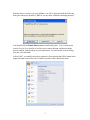
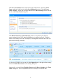
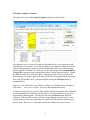
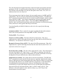
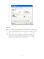
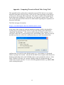
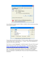
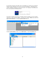
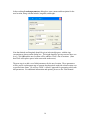
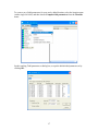
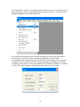
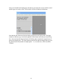
Kansas Geological Survey
Kansas Geological Survey Barometric Response
Function Software User’s Guide
By
Geoffrey C. Bohling, Wei Jin, and James J. Butler, Jr.
Kansas Geological Survey Open File Report 2011-10
August 2011
The University of Kansas, Lawrence, KS 66047 (785) 864-3965; www.kgs.ku.edu
Kansas Geological Survey Barometric Response
Function Software User’s Guide
Open-file Report No. 2011-10
Geoffrey C. Bohling
Wei Jin
James J. Butler, Jr.
Kansas Geological Survey
Geohydrology Section
The University of Kansas Geological Survey
1930 Constant Avenue
Lawrence, KS 66047
Disclaimer
The Kansas Geological Survey does not guarantee this document to be free from
errors or inaccuracies and disclaims any responsibility of liability for
interpretations based on data used in the production of this document or
decisions based thereon.
Acknowledgments
The software described in this report was a product of the calibration monitoring (index)
well program of the Kansas Geological Survey. This program is a pilot study to develop
improved approaches for measuring and interpreting hydrologic responses at the local
(section to township) scale in the Ogallala-High Plains aquifer. The study is supported
by the Kansas Water Office (KWO) with Water Plan funding as a result of KWO’s
interest in and responsibility for long-term planning of groundwater resources in western
Kansas. We thank Bob Buddemeier, Dustin Fross, Ed Reboulet, and Randy Stotler for
their comments on the current and earlier versions of this software.
Introduction
The KGS Barometric Response Function (BRF) software implements the method
discussed in Butler et al. (2011) and Stotler et al. (2011) for computing a BRF and the
method discussed in Stotler et al. (2011) for using the BRF to correct water level (WL)
measurements for the influence of barometric pressure (BP) fluctuations. The software
can also compute earth tide response functions (ETRF) and correct for the influence of
earth tides. However, the calculation of ETRFs is still the subject of ongoing research.
Our preliminary investigations indicate that ETRF estimation can be problematic when
the influence of earth tides is small, so this option should be used with caution. The
appendix describes how to compute theoretical earth tides for a given location using free
software developed at the Royal Observatory of Belgium.
File Management
The KGS BRF software has two components, an Excel worksheet contained in the
workbook KGS_BRF.xls, and a compiled program (executable) named kgs_brf.exe,
both of which are contained in the zip file that includes this document. Questions should
be directed to Geoff Bohling ([email protected], (785) 864-2093).
The Excel worksheet serves as a front end to the executable, providing a template for
managing the water level, barometric pressure, and (optionally) earth tide data. The
worksheet contains three buttons, one to fill gaps in the data records, one to run the
computations for estimating a BRF (and also correct water levels), and one to correct
water levels using a BRF that has already been computed. The Visual Basic code that is
behind these latter two buttons reads information from the worksheet, writes it out to a set
of input files for the executable, runs the executable, and then reads the output from the
executable back into Excel. This means that the Excel worksheet cannot work without
access to the executable. Consequently, a copy of the executable file, kgs_brf.exe, has to
exist in the folder that contains the Excel workbook with which you are working.
You may make copies of kgs_brf.exe using any of the methods provided by Windows
Explorer – selecting an existing copy of the file, then copying and pasting the new copy
in the desired folder, selecting and ctrl-dragging, etc. To see the full file name, with the
extension, you will need to tell Windows Explorer to show you file extensions. But even
if you don’t, the Excel file, KGS_BRF.xls, should be tagged with an Excel icon,
distinguishing it from the executable.
You will likely want to use workbooks that are named something other than
KGS_BRF.xls. The Excel Visual Basic code is directly attached to the Input_Template
worksheet in KGS_BRF.xls. This means that you can make copies of this worksheet
and/or workbook, using any name you please, and the code will be part of each new
copy. This allows you to create and save copies of the Input_Template worksheet using
more meaningful names without “breaking” the software. But, again, you will need to
copy the executable, kgs_brf.exe, to each folder that you work in. You cannot change
the name of kgs_brf.exe because the Excel VB code looks for it by that name.
1
The executable program has been designed so that it can be used on its own, without the
Excel front end. Using it involves creating a set of plain text input files (a parameter file
and input data files) and then running the program in a DOS command window. The
details of this process will be explained in a separate report. The Visual Basic code
attached to the Input_Template worksheet automates the process of generating the input
files and reading the output files.
The Excel workbook (and included Visual Basic code) has been created in Excel 2003. It
should also work in more recent versions of Excel.
Macro Security
To be able to run the Visual Basic code included in KGS_BRF.xls, you may need to alter
Excel’s macro security level from its current setting. In Excel 2003, you set the macro
security level by selecting Options… from the Tools menu, then selecting the Security
tab on the Options dialog box, and then clicking the Macro Security… button on that
tab. On the resulting dialog box, you should set the security level to Medium:
2
With the macro security level set to Medium, you will be presented with the following
dialog box when you open KGS_BRF.xls (or any other workbook containing macros):
You should click the Enable Macros button on this dialog box. If you set the macro
security level to Low, then Excel will just open a macro-bearing workbook with the
macros enabled, without asking for your permission. As noted on the Security dialog
box, this is not advisable.
In Excel 2007, you modify the security options by first selecting the Office button in the
upper left-hand corner of the Excel window to get the Office drop-down menu:
3
Select the Excel Options button at the bottom right on this menu, then select Trust
Center in the list on the left side of the Excel Options dialog box. Click the Trust
Center Settings… button (on the right) and then select Macro Settings from the list on
the left of the Trust Center dialog box:
Select Disable all macros with notification, which is comparable to the Medium
security setting in Excel 2003, then click OK (twice) to get back to Excel. With this
security level setting, Excel 2007 will display a warning below the menu bar when you
open a macro-bearing workbook:
To allow the KGS BRF code to run, click the Options button to the right of the warning
and select Enable this content on the resulting dialog box.
Alternatively, you could choose Enable all macros under Macro Settings in the Trust
Center dialog box. This is comparable to the Low security level in Excel 2003.
4
The Input_Template worksheet
The (upper left corner of the) Input_Template worksheet looks like this:
Hovering the cursor over the cells marked with triangles will reveal comments briefly
explaining the cell contents. To use this spreadsheet, you update the information in the
yellow cells appropriately; paste your measurement time, water level, and barometric
pressure data into columns A-C, starting at row 20; and then press the Compute BRF or
Correct WL button (the latter requires that you have already done the former). Neither
the BRF nor water level correction (WLC) computations allow missing values in the
measurements. If you have gaps in the data, like the WL measurements that are missing
from cells B24 and B25 above, you should fill them using the Fill Gaps button, as
explained below.
Important: The Visual Basic code looks for each piece of information by cell address.
This means . . . don’t move anything. Just revise the information in place.
In order to avoid mixing up your new data with the data that are already in the worksheet,
we recommend that you delete the old data first, by selecting the data from row 20 on
down and then deleting them. Clearing the cells using the Delete button should be
sufficient. If the new data record is as long or longer than the old data record, so that
pasting in the new data will completely overwrite the old data, then the deletion step is
not necessary. However, it is advisable to delete the old data first, just to be sure.
5
The code determines the length of the data record based on the measurement time data
starting in cell A20. It reads down this column from row 20 until it finds a blank cell.
The cell above this first blank cell is the last data point in the record, even if there are
additional data below the blank cell.
The measurement times listed in column A do not actually matter to the BRF and WLC
computations. They are solely for informational and plotting purposes. The BRF and
WLC computations assume that the data are (strictly) regularly sampled, with the sample
interval given in cell B9. Time in these computations is given by the sample interval
multiplied by the sample number (index). The code behind the Fill Gaps button,
however, does use the measurement times and requires that they be in strictly increasing
order (each time is strictly greater than the previous time).
You should modify cells B4-B16 (labels in cells A4-A16) to specify the following
information:
Comment (cell B4): This is a place for user notes regarding the data and/or analysis.
These notes will be passed on to the output BRF and WLC worksheets.
Well (cell B5): The well name.
Water Level Units (cell B6): The units of the WL measurements. This cell is
implemented as a pick list allowing selection from the units listed in cells M5-M6 (feet
and meters). See information about units on page 11.
Barometric Pressure Units (cell B7): The units of the BP measurements. This cell is
implemented as a pick list allowing selection from the units listed in cells P5-P10. See
information about units on page 11.
Earth Tide Units (cell B8): The units of the earth tide (ET) values. This information is
not used if the number of ET lags is set to -1. If ET data are employed, the code will
accept any units that you type into cell B8 and the ET response coefficients will end up
having units of feet per earth tide unit, whatever that unit may be.
Sample Interval (cell B9): The sample interval for the measurements. The BRF and
WLC computations assume that the measurements are regularly sampled at the sample
interval, and ignore the actual measurement time values listed in column A (except when
selecting the data subsets to use for BRF and WLC computations, as described below).
Assuming that these measurement time values are Excel date/time values, then a
convenient way to specify the sample interval is to set cell B9 equal to the difference
between the first two measurement times, that is, cell A21 minus cell A20. This
difference will yield a numeric value, which is in days (e.g., 0.4167 days if the
measurements are one hour apart).
6
Sample Interval Units (cell B10): Or, in other words, the units of time. If the sample
interval is specified as described above (difference between cells A21 and A20, with
those cells containing Excel date/time values), then the sample interval will be in days.
Number of BP Lags (cell B11): The number of lagged values of BP to use in the
analysis. This means the number of values preceding the current WL measurement. A
lag of zero means the BP measurement at the same time as the current WL measurement,
so the number of BP values used in the analysis is the number of BP lags plus 1. You
could set the number of BP lags to 0 to use just the zero-lag BP value – meaning there
would still be something to compute. To exclude BP values from the analysis, you
should set the number of BP lags to -1. You would do this only if you wanted to analyze
responses to earth tides alone.
Number of ET Lags (cell B12): Same as above, except for ET values, instead of BP
values. If the number of ET lags is set to -1, then ET values (column D) are not required
and will be ignored if they are present.
BRF Start Date and BRF End Date (cells B13 and B14): The BRF will be computed
based on a subset of the data measured between the two date/time values specified in
cells B13 and B14. The selection includes these two end points, assuming they
correspond to actual measurement times in the data record. If you have set the number of
BP lags to -1 (only analyzing responses to earth tides), the start and end dates will be for
the ETRF calculation. See further information on selection of start and end dates in
Guidelines for Data Selection on page 10.
Correction Start Date and Correction End Date (cells B15 and B16): The WLC
process will be applied to the subset of data between the two date/time values specified in
cells B15 and B16, again including the end points.
Filling Data Gaps
The BRF and WLC computations do not allow missing values of WL or BP within the
range of measurement times spanned by the BRF or correction start and end dates (cells
B13 and B14 or cells B15 and B16). The same applies to ET values when earth tides are
considered. For the sake of illustration, the WL and BP columns shown in the screen
dump on page 5 include a few missing values. You can use the Fill Gaps button to
interpolate across gaps within the data series, like the gap in the water level series
represented by the empty cells B24-B25. However, the Fill Gaps code will not fill
empty cells at the beginning or end of the record, like the three missing BP values
represented by cells C20-C22, since this would involve extrapolating beyond the
available data.
The Fill Gaps code performs a linear interpolation between the observed data values on
either side of the gap, interpolating to the provided measurement times for the missing
data values. This code requires that the measurement times be in strictly increasing order
7
and will display an error message and stop if they are not. Once it is done running, the
code will present a dialog box showing the number of missing data values that it filled in:
As stated by the dialog box, the interpolated values will be highlighted in red:
The red highlighting is a change to the formatting of the cells and will not go away unless
you change the formatting by some mechanism, such as explicitly changing the format or
pasting in new values with formats included. However, the Fill Gaps code will also set
(or re-set) the font color for non-empty cells to black. The reasoning for this behavior is
that if we pasted in a new data record and then ran Fill Gaps, the black and red font
colors would then correctly indicate the measured and interpolated values in this new
record, even if we hadn’t bothered to undo the red formatting of the interpolated cells in
the previous record. However, a side effect of this behavior is that the code also
eliminates the highlighting of interpolated cells if we run it again on a record that
contains interpolated values. That is, if we ran Fill Gaps again with the worksheet in the
state shown above, then the two interpolated WL values would be taken as “present” (not
missing) and their font would be set to black. The resulting dialog box would also
indicate that the code had filled in 0 WL values. That is, running Fill Gaps more than
once on the same data record will obliterate the distinction between measured and
interpolated values.
Computing a BRF (and Correcting Water Levels)
When you have your data in place and have modified the informational (yellow) cells
appropriately, click on the Compute BRF (and Correct WL) button to
1) compute a BRF based on the WL and BP measurements in the worksheet with
measurement times between the BRF Data Start and BRF Data End date/times
(inclusive) specified in cells B13 and B14, and
8
2) use that BRF to remove (or significantly reduce) the influence of BP variations
from the WL measurements in the worksheet with measurement times between
the Correction Data Start and Correction Data End date/times (inclusive) specified
in cells B15 and B16.
The coefficients of the computed BRF, along with confidence intervals on those
coefficients, will be written out to a new worksheet that is added to the current workbook.
The name of this new worksheet will be BRF n, where n is an integer. The code will
count all the worksheets in the active workbook whose names start with “BRF” and then
set n to that number plus 1. The code will also add a plot to the BRF worksheet showing
the BRF values (equation (2) of Butler et al. (2011)) with error bars.
If ET values are used, then the BRF worksheet will also contain the earth tide response
function (ETRF) coefficients and a plot of ETRF values with the corresponding error
bars.
This new BRF worksheet is yours to do with what you will: rename it, move or copy it,
etc. It contains no links (via formulas) to the original data sheet or to the Visual Basic
code and will not “break” if you move it. Nor does the BRF worksheet contain any VB
code of its own, so if you copied or moved it to a new workbook, you would not be
adding any macros to that workbook (leading to a need to enable macros when you open
that workbook). All the VB code is associated only with the Input_Template worksheet
(or copies thereof). However, if you want to use the BRF contained in this worksheet
later to correct other water levels, then you should not alter the contents of this
worksheet. When you correct water levels using a previously calculated BRF, the WLC
code will expect to find the right information in appropriate cells in the BRF worksheet.
The corrected water levels will also be written out to a new worksheet, which will be
named WLC n, where n is 1 plus the number of worksheets in the current workbook
whose names start with “WLC”. This worksheet will include a plot showing the original
and corrected water levels, along with the BP values (on the secondary Y axis). This
corrected water levels worksheet is also yours to do with what you will. Unlike the BRF
worksheet, there is no need to be concerned about altering the contents of the WLC
worksheet, since it will not be accessed again by the VB code.
The listing of corrected WL values will not start until the number of measurements is
equal to the number of BP lags plus 1. This is because this number of previous BP values
has to be accumulated before the correction can be applied.
Correcting Water Levels (with selected BRF)
It is possible that you will want to correct a series of WL measurements using a BRF
computed using some other series of measurements. You can accomplish this using the
Correct WL (with Selected BRF) button. The correction will be applied to the
measurements in the Input_Template worksheet (or copy thereof), but the BRF
9
coefficients will be read from the worksheet whose name appears in cell J14 (following
the Selected BRF label). Whenever you compute a new BRF, the code will put the name
of the newly generated BRF worksheet into cell J14 on the Input_Template worksheet.
However, you can replace this with the name of any other BRF worksheet by typing the
name of that worksheet into cell J14. The BRF worksheet needs to reside in the active
workbook, but this could be accomplished by copying the BRF worksheet from some
other workbook.
Guidelines for Data Selection
When you compute a BRF, you should do so based on a reasonably stationary data record
that clearly exhibits water level responses to barometric pressure variations, possibly
superimposed on a long-term trend. The same proviso also applies to the estimation of an
ETRF. You should avoid using data records showing abrupt or short-term changes in
water level caused by other factors, such as onset or cessation of pumping, since these
changes could adversely impact the estimation of the BRF (and/or ETRF) coefficients
(see discussion following equation (1) in Butler et al. (2011)). You may apply the
estimated BRF to filter out the influence of barometric pressure variations from more
complicated data records, including those impacted by changes in pumping, as long as
the record you are correcting shares the same barometric response characteristics as those
exhibited by the data used to compute the BRF.
10
Water Level and Barometric Pressure Units
The cells for specifying the measurement units of WL and BP, cells B6 and B7 of the
Input_Template worksheet, are implemented as drop-down pick lists using Excel’s
Validation… option (on the Data menu). Given the number of possible units that can be
used for WL and BP and the challenge of anticipating what combinations are most
probable for this application, the software finesses the issue by converting WL to feet and
BP to equivalent feet of water, performing all calculations in those units, and then
transforming back to the original units. Currently, the list of WL units in cell B6 comes
from cells M5 and M6, which contain “feet” and “meters”. Cells N5 and N6 contain the
multipliers needed to convert each of these units to feet, namely 1 and 3.281. The code
will use the multiplier corresponding to the selected units to convert water levels to feet.
Similarly, the allowed BP units are listed in cells P5 to P10, with the multipliers required
to convert them to equivalent feet of water listed in cells Q5 to Q10. The code will use
the appropriate multiplier to convert BP to feet of water:
Additional options could be added to these lists by adding the label for the units to the list
in column M or P and adding the multiplier for conversion to feet to the adjacent cell in
column N or Q. To add the new units to the drop-down list of options, select either cell
B6 or B7, then select Validation… from the Data menu and expand the list of cells
serving as the Source for the list. For example, to add meters to the list of allowable BP
units, you could type meters in cell P11 and 3.281 in cell Q11, and then use the Data
Validation dialog box to change the Source for the list in cell B7 to include cell P11:
11
References
Butler, J.J., Jr., W. Jin, G.A. Mohammed, and E.C. Reboulet, 2011, New insights from
well responses to fluctuations in barometric pressure, Ground Water, 49(4), 525533.
Stotler, R., J.J. Butler, Jr., R.W. Buddemeier, G.C. Bohling, S. Comba, W. Jin, E.
Reboulet, D.O. Whittemore, and B.B. Wilson, 2011, High Plains aquifer
calibration monitoring well program: Fourth year progress report, Kansas
Geological Survey, Open-File Rept. 2011-4, 175 pp.
12
Appendix: Computing Theoretical Earth Tides Using TSoft
This appendix briefly explains how to obtain the program TSoft and use it to compute
theoretical earth tides for any location. TSoft is a free software package for the analysis
of time series, and gravity data in particular. The software, which was developed at the
Royal Observatory of Belgium, is described in Van Camp and Vauterin (2005). Please
refer to that paper and references therein for further details regarding the computation of
theoretical earth tides.
The TSoft web page is located at:
http://seismologie.oma.be/TSOFT/tsoft.html
At the time of this writing, the software installation package could be downloaded by
scrolling down to near the bottom of this web page and clicking on the link labeled
“Download TSoft Package”. (The current version at the time of this writing is 2.1.12.)
The target of this link is a self-extracting archive named Tsoft_c.exe. After you click on
the link, your browser will ask for confirmation that you want to download the file:
and then either save the file in the default location (e.g., your desktop or a downloads
folder) or prompt for a location. After the file has been saved, navigate to that location in
Windows and double-click on the file Tsoft_c.exe to extract (install) the software. Most
likely, Windows will show you a security warning, asking for confirmation that you
really want to run the extractor. To do so, click the appropriate button (e.g., Run or OK)
on the warning dialog box:
13
You will then be prompted to specify a folder to which the software (and associated data
files) should be extracted:
You can either accept the default folder (C:\Tsoft) or specify a different one by typing in
a different folder name or using the browse (…) button. Then click the Start button to
extract the files to the specified folder.
The Tsoft user’s manual, Tsman.pdf, is available through the “Download TSoft manual”
link near the bottom of the TSoft web page listed above. (The URL for the manual is
http://seismologie.oma.be/TSOFT/Tsman.pdf.) It would make sense to
save this file in the same folder as the software (e.g., C:\Tsoft). The computation of
theoretical earth tides is discussed in the manual’s fourth chapter, entitled “Synthetic
tides”. The remainder of this appendix presents the essential steps for computing
theoretical earth tides at a desired location. Please refer to the TSoft manual for further
information.
14
To start TSoft, navigate to the folder where you installed it (C:\Tsoft if you accepted the
default location) and double-click on the icon for the file tsoft.exe. Depending on how
you have Windows configured, you may not see the “.exe” extension. Nevertheless, the
file’s icon should look something like this:
Once TSoft is running, the first step is to add the location at which you want to compute
earth tides to TSoft’s location database. To do this, go to TSoft’s Tides menu, then select
Open location database… from the Synthetic tides submenu:
In the Location database window, select Add location… from the Location menu:
15
In the resulting Location parameters dialog box, enter a name and description for the
new location, along with the latitude, longitude, and height:
Note that latitude and longitude should be given in decimal degrees, with the sign
conventions as shown on the dialog box. The height should be given as meters above sea
level. Click OK and the new location will be added to TSoft’s list of locations. (Note
that TSoft will replace spaces in the name with underscores.)
The next step is to add a set of tidal parameters for the new location. These parameters
will be used in a subsequent step to compute the theoretical earth tide at that location over
a specified time frame. We will use TSoft’s “default” approach for generating solid earth
tide parameters. For additional information and options, please see the TSoft manual.
16
To create a set of tidal parameters for your newly added location, select the location name
(with a single left click) and then choose Compute tidal parameters from the Theotide
menu:
On the resulting Tidal parameter set dialog box, accept the default tidal parameter set by
clicking OK:
17
Now that you have created a set of tidal parameters, the next step is to create the series of
times at which you want to compute the theoretical earth tide values. To do this, select
Create new data set from TSoft’s File menu:
You will then be presented with a dialog box asking for the time series specification.
Presumably you will want to enter values that will generate a series of times
corresponding to the measurement times for the water level data that you are analyzing.
To generate a series of times at hourly (3600-second) intervals starting from 4:00 pm
(16:00:00) on November 4, 2010, and extending for 120 full days to 4:00 p.m. on March
4, 2011 (2881 hourly samples, including both end points), you would enter:
18
After you click OK on the dialog box, the data set (an empty time series) will be created
and the upper left corner of the TSoft window will show summary information:
Note that the date format used in this display (and in time axis labels in the TSoft plot
window) is dd-mm-yyyy, exactly the opposite of the format used in the previous dialog
box. Also note that the duration shown (120.04 days here) includes the sample interval
past the last sample time. The time span between the first and last sample times is given
by (sample interval)*(number of sample points – 1), or, in this case, (3600 s)*(2880) =
120 days.
19
Now that you have generated the series of sample times, return to the Location database
window (opening it if necessary by selecting Open location database… from the
Synthetic tides submenu of the Tides menu, or using the Shift+L keyboard shortcut),
select (single click) the location name on the left (Thomas_Co_IW in our example), and
then select (also with a single click) the synthetic tide parameter set on the right (WDD):
Take a moment to make sure that both the desired location and the synthetic tide
parameter set are highlighted, and then select Calculate from the Theotide menu:
Once you click Calculate, the code will compute the theoretical earth tide values for the
selected location and specified times.
20
The computed values will be added as a new “channel” in the time series. You can
display these values in the plot window by clicking on the leftmost of the two squares
next to the channel name:
To export the computed values from TSoft, click the rightmost of the two squares next to
the channel name. It will turn red to indicate that the channel is selected for export. Then
select Export channels from the File menu. This will generate a plain text file named
expchan.dat. For this example, the first few lines of this file contain:
7383
7384
7385
7386
7387
7388
7389
7390
7391
97.1388935
-50.1369591
-31.3465880
148.4776570
433.5105504
732.7225562
945.0343588
986.9680693
815.4135353
The first column contains a sample time index and the second column contains the
theoretical earth tide value for that time, in nm/s2 (nanometers per square second).
According to the manual, the time index represents the “number of sample intervals since
the first January of the first year of the current data series.” A bit of experimentation has
shown that the proper way to translate this index into the appropriate date/time value in
Excel is essentially:
21
sample time/date = (1/1/yyyy 0:00) + (sample interval in days) * (index + 1)
where yyyy is the year containing the first sample time in the series. In this example, if
we import expchan.dat into Excel (as a space-delimited text file), and add a couple
headers, we get:
Since the series starts in 2010, we can add sample times by entering midnight of Jan 1,
2010, as an “anchor” for the calculations, then generate a column of times using the
formula above, formatting the results as date/time values:
The first sample time, in cell C2, is highlighted, and its formula appears in the formula
bar above. $E$2 refers to the date in cell E2, with the dollar signs to fix that cell address
as you fill down the column, (1/24) is the sample interval (one hour) expressed in days,
and (A2+1) is first cell index plus 1. This generates a sample time that corresponds to the
22
series start time shown in TSoft, and pulling down the formula to the last sample
generates the intended end time of 3/4/2011 16:00:
Generating a column of sample times in this fashion will help you confirm that you are
properly matching up the computed earth tides with your water level measurements.
Once you have done so, you can transfer the earth tide values column D of the
Input_Template worksheet in KGS_BRF.xls (or a copy thereof) by copying and
pasting.
Reference
Van Camp, M., and P. Vauterin, 2005, Tsoft: graphical and interactive software for the
analysis of time series and Earth tides, Computers & Geosciences, 31(5), 631-640.
23