Download njit-etd1991-017 - New Jersey Institute of Technology

Copyright Warning & Restrictions
The copyright law of the United States (Title 17, United
States Code) governs the making of photocopies or other
reproductions of copyrighted material.
Under certain conditions specified in the law, libraries and
archives are authorized to furnish a photocopy or other
reproduction. One of these specified conditions is that the
photocopy or reproduction is not to be “used for any
purpose other than private study, scholarship, or research.”
If a, user makes a request for, or later uses, a photocopy or
reproduction for purposes in excess of “fair use” that user
may be liable for copyright infringement,
This institution reserves the right to refuse to accept a
copying order if, in its judgment, fulfillment of the order
would involve violation of copyright law.
Please Note: The author retains the copyright while the
New Jersey Institute of Technology reserves the right to
distribute this thesis or dissertation
Printing note: If you do not wish to print this page, then select
“Pages from: first page # to: last page #” on the print dialog screen
The Van Houten library has removed some of the
personal information and all signatures from the
approval page and biographical sketches of theses
and dissertations in order to protect the identity of
NJIT graduates and faculty.
OFF-LINE PROGRAMMING USING IGRIP
by
NARAHARI K. BHANDARY
Thesis submitted to the faculty of the Graduate School of
the New Jersey Institute of Technology in partial fulfillment of
the requirements for the degree of
Master of Science in Mechanical Engineering
1991
APPROVAL SHEET
Title of Thesis
: OFF-LINE PROGRAMMING USING IGRIP
Name of candidate : Narahari K. Bhandary
Thesis and Abstract
approved by
Date
Prof. N.Levy/
Associate Professor
Department of Mechanical Engineering
Faculty Committee
Date
Prof. D.Lubliner
Adjunct Assistant Professor
Department of Manufacturing Engineering
Prof. M. Leu Date
Professor
Department of Mechanical Engineering
VITA
NAME
: Narahari K. Bhandary
DEGREE AND DATE TO BE CONFERRED : M.S.M.E., October 1991
MAJOR
SECONDARY EDUCATION
: Mechanical Engineering
: Central School(KVM)
Mangalore, India 1982
POST SECONDARY EDUCATION
DATES DEGREE DATE OF DEGREE
COLLEGE
New Jersey Institute of
Technology, Newark
9/89 - 5/91
MSME
Sri Jayachamarajendra College
of Engineering, Mysore
9/84 - 11/88
BSME
Oct. 1991
Nov. 1988
ABSTRACT
Title of Thesis
: OFF-LINE PROGRAMMING USING IGRIP
By
: Narahari K. Bhandary, MSME, 1991
Thesis directed by : Dr. N. Levy
Department of Mechanical Engineering
AT&T's FWS-200(Flexible Work Station) has been modeled and simulated to implement Off-Line Programming(OLP). IGRIP(Interactive Graphics Robot Instruction
Program) from Deneb Robotics, Inc. has been used to simulate the FWS operation.
A GSL(Graphics Simulation Language) program has been used to simulate the chip
placements during PCB assembly. The program leads the user through the motions of
chip placement, and after the simulation run downloads the motion sequence to the FWS.
The animation sequences of the FWS have been downloaded to the FWS on the
Factory Floor using a C program, which is utilized to communicate the data to an M 2 L
program on the FWS. An awk program is used to take care of the handshake protocol
between the Silicon Graphics workstation running IGRIP and the 80386 PC running
M 2 L.
The use of simulation has been observed to help the user in visualizing the sequence
of chip placement. OLP offers a naive user the option of running the FWS without
learning M 2 L, and an experienced user significant savings in programming time and a
testbed for optimization.
ACKNOWLED GEMENTS
I would like to acknowledge Prof. N. Levy's role in this venture of mine and thank
him for his suggestions during the course of this thesis. I wish also to acknowledge the
Graduate Advisor, Prof. H. Herman and the Chairman, Dr. B. Koplik for their support.
I would like to take this opportunity to express my gratitude to Prof. D. Lubliner for his
invaluable guidance and moral support available to me all through. Without his backing
and encouragement at all times(which is highly appreciated), this thesis would never have
been. I would also like to thank Prof. M. Leu for his helpful suggestions.
Contents
1
1
2
2
3
3
1 Introduction
1.1 Simulation 1.2 Off-Line Programming 1.3 IGRIP 1.4 AT&T FWS 1.5 Objective 2 AT&T FWS-200
2.1 General Overview 2.1.1 Hardware Description 2.1.2 MML 2.2 Power-Up Sequence 2.3 MML Procedures 2.4 Power-down sequence 5
5
6
9
9
10
15
3 Simulation
3.1 Introduction 3.2 Characteristics of a simulation system 3.3 IGRIP
3.3.1 CAD 3.3.2 DEVICE 3.3.3 Setting up DEVICE Kinematics 3.3.4 WORKCELL Layout 3.3.5 Tag Points 3.3.6 Input/Output Signals 3.3.7 PROGRAM 3.3.8 GSL Programs 3.3.9 MOTION 16
16
16
17
20
20
22
25
26
27
28
33
63
4
65
65
66
66
Off-Line Programming(OLP)
4.1 Introduction 4.2 OLP 4.3 Principles of OLP ii
4.4 OLP Systems 4.4.1 CAD system 4.5 OLP software 4.6 Postprocessor
4.6.1 C Program 4.6.2 AWK 4.7 OLP Benefits 67
68
71
72
72
74
76
5 Simulation Run
5.1 Simulation Setup 5.2 Running the simulation 5.3 Output File 78
78
79
85
6 Conclusions
89
7 Recommendations
90
Appendix A
91
Appendix B
93
Glossary
97
Sources Consulted
100
List of Figures
7
8
2.1 FWS 2.2 CONTROL PANEL 4.1
OLP Schematic 70
5.1
5.2
5.3
5.4
5.5
5.6
AT&T FWS-200 Simulation Run: Step 1 Simulation Run: Step 2 Simulation Run: Step 3 Simulation Run: Step 4 Simulation Run: Step 5
80
81
82
83
86
87
iv
Chapter 1
Introduction
1.1
Simulation
Simulation is the technique of constructing and running a computer model of a real
system in order to make a dynamic analysis without disrupting its environment, prior to
its implementation.
Simulation provides requisite information to determine the feasibility of a system
by studying it under totally dynamic conditions. It is used to construct and display
mathematical models with the same constraints as those of the actual robots, so as to
manipulate and visualize the three dimensional models accurately. It is also a real time
analysis and control tool as it allows the designer to visualize motions at every stage of
the cycle in real time. It also helps an engineer select the best robot for the job based
on interference checks, and reachability of various points in the workcell. Various studies
like cycle time analysis and collision detection help in optimization.
Simulation is one of the best ways to design an integrated, complex robotic workcell.
It reduces the overall design time and increases the probability of success of the workcell
implementation.
1
2
1.2 Off-Line Programming
Off Line Programming(OLP) is the technique of developing a computer program
-
without involving the robot itself in the programming process to run a robot from a
remote site.
Robots have conventionally been programmed by 'teach-by-show' methods which
involve using a teach pendant and are sometimes slow and tedious. These involve stopping
the assembly line for the duration of the teaching process to incorporate any changes.
On-Line Programming involves coding and debugging on the machine which is trying
and time-consuming, also it hinders production.
Off-Line Programming is essential in CIM(Computer Integrated Manufacturing ).
It is very helpful in factory floor operation as it doesn't interfere with production. It can
prove very helpful if the assembly operation isn't fixed, especially in a FMS (Flexible
Manufacturing System) environment, where reprogramming for different specifications
can be very time-consuming and tedious.
OLP assumes a great significance on account of its several advantages. It does away
with the teach pendant altogether. It uses simulation and animation data to develop the
robot program which can be modified very easily if required. Once the workcell undergoes
some test runs, the probability of success of the program on the actual workcell increases.
The workcell need be taken out of production only when the program is ready for testing.
The program can be tested immediately by downloading it to the workcell via a hard
wired connection, the network (if a card is present), or some transfer media like floppy
disks.
1.3 IGRIP
IGRIP (Interactive Graphics Robot Instruction Program) from Deneb Robotics, Inc. is
3
a simulation/animation package used for workcell layout, simulation, and OLP.
IGRIP consists of a CAD section, a Device modeler and a Layout section. Parts
are modeled in the CAD section using primitives like cone, block, sphere, pipe, cylinder
etc. Devices with multiple degrees-of-freedom comprising Parts are defined in the Device
section. These Devices are laid out with I/O signals set up between them in the Layout section. Simulation is carried out by running GSL(Graphic Simulation Language)
programs in the Motion section.
1.4 AT&T FWS
The AT&T FWS-200 is a 4-axis gantry-style, pick-and-place robot with two types of
manipulators - one with a vacuum tool, the other with a tool changer accommodating
a vacuum tool and a gripper. It is programmed in a multitasking, modular, BASIC-like
control language, M 2 L (Modular Manufacturing Language), and controlled by a 80386based PC.
1.5 Objective
The objective of this work is to enable communication between the simulation system,
IGRIP, and the FWS on the factory floor. This involves overcoming the handshake
protocol between the different hardware devices involved. Serial communication requires
protection against data loss during transmission. As the FWS is not a member of the
library of robots in IGRIP, the kinematics of the manipulators need to be set up.
The work in this thesis can be broadly classified into two sections. In the first, the
simulation setup was designed. This involved modeling of the AT&T FWS-200, setting up
the kinematics of the manipulators, and programming of the FWS simulation setup using
GSL. The second part involved the setting up of a physical communication link between
4
the Silicon Graphics Workstation on which the IGRIP software resides and the FWS on
the factory floor via a RS-232 cable running between their serial ports; programming
to enable communication between the simulation system, IGRIP, and the AT&T FWS
using C.
The following chapters discuss how the AT&T FWS-200 has been modeled, simulated
and programmed off-line from the simulation software IGRIP.
Chapter 2
AT&T FWS-200
2.1 General Overview
The AT&T FWS-200 (Flexible Work Station) is a pick and place robot with a built-in
operator interface, and programmed in a multitasking control language, M 2 L, Modular
Manufacturing Language.
The FWS-200 is an overhead gantry style, four-axis robot primarily used for precise
positioning of light to moderate weight work pieces. It supports multiple manipulators
within a common workspace. It can be easily customized, and can function as a standalone unit or as an integrated part of an assembly line.
The FWS is modular in design and equipped with an user programmable touchscreen interface. A 80386 based PC is used for robot system control. The Modular
Manufacturing Language, M 2 L, is a modular, BASIC-like language which allows multitasking control of the robot and other equipment such as machine vision systems.
The FWS has two manipulators: one with a vacuum tool and a camera, the other
with a tool changer accomodating a gripper and a vacuum tool. It also includes an
up-looking camera connected to an IRI SVP 512 vision system.
The FWS's main application is placement of a variety of components into a printed
circuit board. Both through-hole and surface mount components are placed with the
5
CHAPTER 2. AT&T FWS-200
6
surface mount parts ranging from 25 to 50 mil pitch. The through-hole parts are picked
from a feeder and mechanically nested before placement. If the part does not immediately
insert, a spiral search pattern called vibratory insertion is used until the part drops in.
The 50 mil pitch surface mount devices are also mechanically nested. The 25 mil pitch
surface mount devices are visually nested before placement.
The manipulators can quickly accelerate to a velocity of 60 inches per second yielding
a typical part acquisition-placement cycle of 2 seconds per part per manipulator. The
maximum velocity of the X- and Y-axis is 75 inches per second but in practice, it averages
around 30 inches per second.
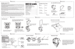
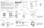
2.1.1 Hardware Description
The control cabinet houses
• Control display - system power buttons, touch display, pressure and vacuum gauges,
and emergency stop button
• 80386-based PC - controls the FWS
• Manipulators - provide X, Y, Z, & 0 motion of the system.
• Pneumatic & ventilation systems
• Power supplies
• Axes control electronics
• Industrial I/O modules & STD bus
FLEXIBLE WORK STATION
Figure 2.1
CONTROL PANEL
Figure 2.2
CHAPTER 2. AT&T FWS-200
9
2.1.2 MML
M 2 L is an interpretive language. The interpreter reads and executes one line of a program
at a time immediately and, without requiring an intermediate compilation phase.
M 2 L is :
• Familiar: BASIC-like syntax
• Multitasking: can handle many tasks simultaneously while supporting communication and synchronization between various tasks
• Flexible: can be customized to control any machine or process and is not restricted
to just robot control
• Portable: easily portable as it's written in C
• Full Featured: equipped with a full screen editor, debugger and support for other
editors like vi
2.2 Power-Up Sequence
To turn the FWS on:
1. Turn on the power by pressing the Emergency Reset ON pushbutton. The fans
will turn on and the Emergency Reset POWER light will illuminate.
2. Turn the Main Power Key Switch to the ON position.
3. Turn on the computer by pressing the Computer ON pushbutton. The Computer
POWER light will illuminate, and the computer will boot up.
4. Turn on Servo #1 and Servo #2 by pressing the START pushbuttons. The
Servo lights will illuminate .
CHAPTER 2. AT&T FWS-200
10
5. Press the AIR ON pushbutton. The AIR light will illuminate. The air valve
will open supplying air pressure to the system. Note: If the air pressure is
insufficient(<85 psi), the INTERLOCK fault light will illuminate.
6. Check INTERLOCK light, if it is lit, close any open drawers, safety shields, or
correct the air pressure.
2.3 MML Procedures
There are three methods of executing a procedure in M 2 L.
• The run command runs the procedure with all the currently defined variables available to it.
run [procname] [(arglist)]
where procname is the name of the procedure to run, and arglist is a list of arguments separated by commas.
• The call command also runs the given procedure, but in a different data space.
This means that any variables that the procedure creates will be gone when the
procedure returns.
call procname[(arglist)]
• The debug command is identical to the call command, except that execution is
suspended before each line of the procedure in order for you to inspect variables,
set breakpoints, etc.
debug procname[(arglist)]
The procedure "corn" is used to configure the serial port of the PC running M 2 L.
The procedure "demorun2" is used to read the data sent over the RS-232 cable from
the SGT, to be subsequently used in carrying out the motions of the manipulators. The
CHAPTER 2. AT&T FWS-200 11
program is invoked by typing 'run cdemo' at the mml prompt on the FWS (after the
power-up sequence).
procedure com
sdefine ""coral"
' Defines the device called coral i.e, the serial port
stype "com1"
' Uses the device handler called coma for the device previously
' defined with the sdefine command
sset "port", 1
sset "baud", 9600
sset "parity", "even"
sset "size", 7
sset "stopb", 1
sset "enable", 1
' Sets the database fields(name, base, port, avail, baud,
' parity, size, or stopb) to their respective values
procedure demorun2
loadg datapts
' Loads the geometry variables from the file named datapts .v
call com
' Calls the procedure called com
CHAPTER 2. AT&T FWS-200
int a = 0
string s = ""
string i = ""
string j = ""
int errflag = true
int rob = 1
string tol = "vac"
point safpt = sp1
point pp
point cpoint
point plpoint
offset over = offset( 0, 0, 0.5, 0 )
sopen "coma"
' Opens a connection to the device called coma
while j <> "END"
s = sgets( "com1" )
' Obtains a string s from the SIO device called com1
i = strtok( s, "*" )
' Is the first invocation of strtok() that is to be used
' The string s is passed along with the delimiter *
j = strtok( ":" )
wend
sclose "com1"
' Closes the connection to the device called coma
fopen "i", 3, "testy.dat"
' Opens the file whose name is testy.dat using mode i(input)
12
CHAPTER 2. AT&T FWS-200 ' And file identifier 3
j =
while j <> "END"
fline_input 3,s
' Places all the characters of a line from the file pointed to by
' 3 into the mml string s
i = strtok( s, "*" )
j = strtok( ":" )
k = strtok( "x\n" )
switch j
case "SPEED"
speed val(k), val(k), val(k), 500
' Sets the speeds in in./sec for X,Y,Z and deg/sec for theta
case "OFFSET"
offset over = offset( 0, 0, val(k), 0 )
case "ROBOT"
if k = "1" then attach "1"
' Will cause manipulator 1 to be attached to the mml interpreter and
' Also cause it to be completely initialized
if k = "1" then tol = "vac"
040
if k = "2" then a = 1
call home
' Calls the procedure called home
if a = 1 then call gettool( 2, "grip" )
' Calls the procedure called gettool to pick up the gripper from
13
CHAPTER 2. AT&T FWS-200
' the tool changer
if k = "2" then imove -4,0,0,0
' Moves the manipulator 4 inches away from the tool changer
a = 0
if k = "1" then rob = 1
case "SAFE_POINT"
if k = "sp1" then move sp1
break
' Used to insure that the move has been completed
if k = "sp2" then safpt = sp2
case "PICK_POINT"
if k = "ch10" then pp = ch10
call pick( pp, over, tol, errflag )
' Calls the procedure pick
case "CHECK_POINT"
if k = "cp1" then cpoint = cp1
4.0
move cpoint+over
move cpoint
move cpoint+over
case "PLACE_POINT"
if k = "ch310" then plpoint = ch310
14
CHAPTER 2. AT&T FWS-200
call place( plpoint, over, tol, errf lag)
' Calls the procedure place
move safpt
endsw
wend
fclose 3
' Closes the file with file identifier 3
2.4 Power-down sequence
To power-down the unit:
1. Press the AIR OFF pushbutton.
2. Press the Servo #1 and Servo #2 OFF pushbuttons.
3. Turn the Main Power Key Switch to the OFF position.
15
Chapter 3
Simulation
3.1 Introduction
Interactive computer graphics for simulation and Off-Line Programming is a powerful
tool for implementing robotic applications. Simulation systems provide significant time
savings in the layout and modeling of robotic workcells. Furthermore, as manufacturing
equipment becomes more complex and costly, these systems provide added assurance in
cell layout optimization. It has been estimated that 60% - 80% of the task of implementing a robotic workcell is devoted to cell layout, equipment design, robot selection, and
hardware mockup of the workcell. Remaining efforts are in the programming and actual
implementation on the factory floor.
The general characteristics of a simulation system as well as the salient features of
the IGRIP, the simulation system used in this work, are discussed.
3.2 Characteristics of a simulation system
The main objectives of a simulation system:
• Improved Accuracy
• Improved Communication
16
CHAPTER 3. SIMULATION 17
• Reduced Development Time
A simulation system should have good graphics capabilities as well as a solid modeling module so that the user can validate the model for accuracy and completeness.
It should also allow the import of standard file formats such as ICES (Initial Graphics
Exchange Specification). The system should be user-friendly to enable easy, interactive
modeling and simulation. Ability to simulate different operations like painting, welding,
etc., is desired to increase the system's versatility. Features like collision detection and
cycle time analysis are a must to assist in optimization. The user should have access to a
database of the most commonly used robots. The system should be able to simulate the
kinematic and dynamic behavior of the robots. The simulation system should possess the
capability of interfacing with the shop floor equipment so as to download the simulation
sequences directly to the robot controller.
Simulation should be continued even after workcell implementation on the shop
floor for optimization. The underlying philosophy is to provide a dynamic, interactive
environment on a high-performance engineering workstation and to be able to shorten
the design/evaluation cycle as well as optimize the operations.
3.3 IGRIP
IGRIP TM is a user-friendly computer graphics based simulation system for workcell layout, simulation and off-line programming (OLP). Parts modeled within the Part Modeler
(CAD Context) are put together to define Devices with multiple degrees of freedom. A
Device has both geometric and non-geometric information stored with it. Non-geometric
information like kinematics, dynamics, velocities etc. can be entered through interactive menus. A Workcell is composed of Devices, positioned relative to each other
(WORKCELL Context). Devices may be selected from a library of robots, conveyors,
CHAPTER 3. SIMULATION
18
end-effectors or modeled by the user in the DEVICE context. IGRIP has the capability
to generate robot programs interactively (MOTION Context). Several Devices may be
simulated simultaneously with Input/Output signaling set up between them.
The IGRIP menu system is divided mainly into Contexts, which are arranged across
the top of the IGRIP screen, each of which has a group of subdivisions called Pages. The
Contexts are :
• CAD The CAD Context allows the user to create and modify 3-D surface or
wireframe geometry used to represent Parts.
• DEVICE The DEVICE Context allows the user to build and modify Devices by
putting together the Parts built in the CAD context.
• LAYOUT The LAYOUT Context allows the user to lay out a workcell. This
includes positioning Devices, creating Paths for motion definition, connecting I/O
signals and creating Collision Queues.
• MOTION The MOTION Context allows the user to define and execute motion
for Devices. Motion can be commanded interactively or through Program control
(when running a simulation). Simulation Programs can also be downloaded to
specific controller or generic formats.
• DIMENSION The DIMENSION Context allows the user to create and manipu-
late various kinds of dimension entities to document workcell layouts and geometric
data. Dimensions are fully three dimensional planar entities, and can be translated
and rotated in space with respect to a coordinate system that is local to the dimension. Dimensions are also dynamically associative, or "data-driven", which implies
that the dimensions are attached to geometry, and are continuously updated to
reflect the current state of that geometry.
CHAPTER 3. SIMULATION
19
• USER The USER Context allows customization of the user interface to define
custom Menu Pages with functions taken from other Pages, or functions to invoke
CLI(Command Line Interpreter) macro files.
• ANALYSIS The ANALYSIS Context allows the user to perform various forms of
analysis. Functions on the MEASURE Page allow identification of various items in
the world, as well as the determination of the distances and angles between them.
The units for reporting as well as the frame of reference may be set by the user.
Entity properties such as area and volume may be queried using functions on the
PROPERTIES Page. All analysis functions utilize "Analysis Registers" that can
be used in conjunction with IGCALC. Some of the Registers and the data values
they represent are :
— c: Value of the current Popup field
—p: Last value entered
— x, y, z x-, y-, and z-coordinate of a point respectively
— dx, dy, dz: Distance in the x-, y-, and z-direction respectively
— d: Total Cartesian distance
— V: Object volume
— A: Object area
— dia: Polygon diameter
- ang: Angle between entities
— R, P, Y: Roll, Pitch, and Yaw angle about Z-, Y-, and X-axis respectively
• SYSTEM The SYSTEM Context provides system utilities to modify the system
environment and world attributes as well as to interact with the UNIX file system.
CHAPTER 3. SIMULATION
20
• CLI The CLI( Command Line Interpreter ) Button is used to enter CLI commands
interactively. This enables the expert user to type in a command from any Context
without switching to the relevant Context.
3.3.1 CAD
Before beginning the design of Parts, the units should be set up (if other than the default,
mm, is desired) as below :
• Select the ANALYSIS context. Select the UNITS Button and enter the new units
in the Popup (or use the LMB to select from the choices). The new units will be
used for all subsequent operations.
• To actually design the Parts, select the CAD context and click on the CREATE
Button to go to the CREATE page. The CAD context is used to model the geometry used to design Parts, which consist of one or more Objects which in turn
comprise one or more Subobjects composed of Lines and Polygons.
• Objects are created using the CAD primitives Block, Cylinder, Cone, Wedge, Pipe,
and Sphere. These Objects are modified using the CAD operators such as Cut,
Mirror, Loft, Clone, Extrude & Revolve. From MODIFY page, use Merge, Smash,
Scale, Cut, Color Object, and Extract Obj to further modify the Objects. From
Auxiliary page, create Coorsys to assist in attaching subobjects to make up an
Object.
3.3.2 DEVICE
To build a new Device, use the following procedure:
• Select the DEVICE Context, then the NEW DEVICE Button. You will be placed
in the Syslib/PARTS directory. Select the appropriate directory in the Popup to
CHAPTER 3. SIMULATION
21
move to your directory.
• Select the Part to be used as the base of the new Device.
• Enter a name for the Device and accept the defaults for the Device parameters in
the Popup.
• Select the AXES Button, then pick the Part that was just retrieved, to force the
Coorsyses to always stay visible.
• Select the ATTACH PART Button and then pick the base of the Part to indicate
the Part that the new Part will be attached onto.
• Choose the other Parts and then the key Coorsyses, placed in the CAD Context to
facilitate easy positioning of the Parts.
• Select the KIN Page, and select the JOINT TYPES Button. This is where the
Translational vs Rotational dof are assigned at each joint. Change the first three
to be Translational and accept the default, Rotational for the other three joints.
• Select the SET DOF Button and pick the Part which is supposed to move along
X- and/or Y-axis. The "Link Transformation" Popup is used to describe how the
Joint should move. The most common choices are to Translate along an axis, or to
Rotate about an axis.
• First specify "Set Home", next specify "Trans X", enter a 1 for the "Translate X
Expr:", finally select "Return". The "Set Home" option indicates that the system
should use the current location and orientation as the "zero" position when calculating the location. The "Trans X" option defines motion along the Part's X axis.
This motion is tied to Degree of Freedom number 1. In other words, Joint 1 is
a Translational Joint that moves positive in the Part's positive X direction. The
CHAPTER 3. SIMULATION
22
"Return" choice completes the DOF definition. It is possible to have more than one
DOF number for the same Part, as also to have one DOF number control motion
for many Parts, in many different directions, as well as mixing types of motion.
• Select the other Parts and repeat the above except choose "Trans Y", "Trans Z",
"Rotate Z", "Rotate Y", and "Rotate X" with DOF numbers 2,3,4,5,and 6 respectively.
• Now select the KINEMATICS Button and choose the "Inverse Kinematics" option
from the Popup.
3.3.3 Setting up DEVICE Kinematics
To begin with, the manipulators were assigned Simple Kinematics. It was observed
that the Device split up into its constituent Parts while moving to a Tag Point.
The Utool did align with the Tag Point, but as the FWS is an overhead gantry
style robot, Simple Kinematics was not suitable for the purpose. Then, the Generic
kinematics method was used, and finally the Device Kinematics method was used.
There are 2 methods of configuring the manipulators of the FWS-200, one by using
an inverse kinematics routine from the IGRIP library and two by using Generic
Kinematics. To model a new Device the kinematics of any of the existing Devices
can be used, if the following conditions are satisfied:
1. The base coordinate systems for each part on each Device must match exactly.
The positive/negative directions of rotation must be identical.
2. The number of dofs for both Devices must be same.
3. The type of dof must be the same in both Devices(i.e., ROTATIONAL vs
TRANSLATIONAL).
CHAPTER 3. SIMULATION 23
Selecting 'Device Kinematics' from the displayed Popup allows the user to select
any Device existing in the DEVICE directory. The Device being built will assume
the kinematics math-routine defined for the Device name selected from the file-list
Popup. Note that if any of the parameters mentioned above (link lengths, link
offsets, link types, mounting plate offset, or DOF definition) do not match those of
the selected Device, the new Device will not be able to reach its points.
— Select JOINT LENGTHS. This is where the D.H. parameters(The Denavit
Hartenberg notation is used to represent the robot kinematics parameters.
The gist of this is to represent the robot kinematically using link lengths
and offsets based on the coordinate system of each link fixed at arbitrary
locations. i.e, lengths between base coordinate systems as well as offsets from
the principal plane ) are assigned.
— Select BASE PRT and pick the Part of the Device which is to serve as the
base. Use UFRAME under the MOTION Context to verify by picking the
`Display' option from the Popup, that the UFRAME is the base Coorsys of
the Base Part.
— Select the MNT FLT Button. Here the user graphically selects the part
which represents the Device mounting plate and defines the offset values. Use
UTOOL Button under MOTION Context to set the Tool Point. Pick 'Display'
from the Popup and verify the Tool Point.
— Select HOME POSITION Button and set the home position to be the current
Joint value by choosing the "Use Current Position" option in the Popup.
— Select the SPEEDS Button located under the LIMITS Title and complete the
Popup.
— Select the ACCELS Button and set the maximum accelerations.
CHAPTER 3. SIMULATION
24
— Select the TRAVEL Button and set the travel limits.
— This completes the definition of the new Device. If any modifications are
necessary, use REDEFINE DEVICE Button and make the requisite changes
in the Popup.
— Finally, select SAVE DEVICE Button and complete the Popup with the name
of your directory and the filename.
The Generic Kinematics method can be used to model a new robot with any number
of degrees of freedom (dofs). It is very slow to execute as compared to the closed
form solutions on account of it uses an iterative approach which only searches for
solutions which lie within the specified link limits. It can provide a solution where
other methods fail, but at the same time it doesn't always come up with a solution
even when one exists. To setup the FWS manipulator using Generic Kinematics:
— Select the DEVICE context, then select the Attributes Button to go to the
Attributes menu Page.
— Select LINK TYPES and choose "Translational" for the first three joints and
"Rotational" for the other three joints.
— Select DOF( This allows one to define the type of transformation being applied
at each joint). Choose the top part of the manipulator, click on "Set Home"
in the Popup, then click on "Trans X" and type in 1 in response to the Popup
and finally click on "Return". This signifies that the first dof is translational
along the X-axis. Repeat the above sequence except this time choose "Trans
Y" and type in 2. Next choose the middle part of the manipulator and repeat
in the same order by choosing "Trans Z" and typing 3. Then choose the
bottom part of the manipulator and choose "Rotate Z" and type in 4 in the
CHAPTER 3. SIMULATION
25
same order. Finally, choose the bottom plate at the tip of the tool and choose
"Rotate Y" as 5 and "Rotate X" as 6 in the same sequence.
— Select KINEMATICS and choose "Generic" from the Popup.
— Select MNT PLT and choose the plate at the tip of the tool.
— Select BASE PRT and choose the plate attached to the top of the manipulator.
— Select GENERIC KIN and choose "Cartesian class".
— Select JOINTS PRESENT and choose "All 6 Present".
— Select OFFSETS and type in 0.5 for 1 & 2, 16.11 for 3 and 0 for the rest.
— Select WRIST ROTN and type in -90 for "Roll Offset" (Z Rotn).
3.3.4 WORKCELL Layout
To layout a Workcell, follow the steps below:
• Select the LAYOUT Context and the WORKCELL Page.
• Select the RETRIEVE DEVICE Button. Choose your directory from the Popup,
and pick the relevant Device.
• Select the AXES Button; this will toggle the Device's display mode so that it's
Coorsyses are always displayed.
• Select the RETRIEVE DEVICE Button again to pick the other Devices to be laid
out in the Workcell.
• Select TRN DEV or ROT DEV to arrange the Devices in the Workcell. The SNP
Button is a quick way to do 90 degree rotations about the primary axis. The LMB
rotates about X, MMB about Y, and the RMB about the Z axis. If any Devices are
CHAPTER 3. SIMULATION
26
to be attached to another Device, select SNAP DEV Button. Choose the 'Frame'
option from the "Snap Device On..." and pick the Coorsyses on the Device.
• Select the ATTACH Button using the MMB (Middle Mouse Button). This will
give a list of all the Devices that are currently in the Workcell. Choose a Device
and pick a part on the Device to attach it to. The part should highlight and any
Coorsyses, if present, will appear. Pick the right Coorsys and the Device will snap
onto the part using the orientation of the Coorsys.
• At this point, the locations and orientations of each Device should be saved. Move
to the SYSTEM Context, WORLD Page, and pick the SAVE POSITIONS Button.
Choose the "All Devices" option from the "Save/Restore Positions" Popup. This
establishes "Restore Positions" for the location and the Joint values of each Device.
This can be used as the starting point when running simulations. If this is not done,
when the simulation is RUN using "Previous Values" all the Devices jump to the
World Origin.
• Use the World Display functions to move to a view of the Workcell that shows most
of the Devices, and save the Workcell using SAVE WORKCELL Button.
3.3.5 Tag Points
Tag Points are primarily used to indicate destination positions for robot motion. The
user places Tag Points at the desired location and orientation and then, instructs the
robot to move to the Tag Point position.
Tag Points may be set up as follows:
• Select the LAYOUT Context and then the RETRIEVE WORKCELL Button.
Choose the Workcell from the Popup.
CHAPTER 3. SIMULATION
27
• Select the TAGS Page and then the NEW PATH Button, pick the Device to attach
the Path to.
• Select the SETUP Button and complete the Popup. This allows you to constrain
or free the Degrees of Freedom.
• Select the SURFACE Button and then, using the LMB (Left Mouse Button), pick
the surface to snap the Tag Point onto. You may also select the VERTEX, EDGE,
FRAME Buttons as appropriate.
• If the orientation of the most recently created Tag Point is desired for subsequent
Tag Point placements, pick the surface with the RMB (Right Mouse Button). This
will place a new Tag Point at that position with the same orientation as the previous. If your Tag Point names end in integer numbers, the new Tag Point will be
added to the current Path and given the next available ending number.
If only part of the Tag Point is visible, part of it is hidden inside of the polygon. You
may want to go to the SYSTEM Context and select the Z-BUFFER Button, it should
dehighlight (which means the real time Z-Buffer is turned off) and all of the Tag Point
axes become visible.
This completes the Path layout. To check on the reachability of these Tag Points,
select the T-JOG Button. Pick the Device (Robot) to be T-Jogged when the Tags are
moved. Now the Device will move to any Tag Point picked, align itself to the Tag Point
using its Utool, and follow it. The Tag Points can be selected one by one to check position
and orientation. If needed, any changes may be made using TRN TAG and ROT TAG
Buttons.
3.3.6 Input/Output Signals
To layout the I/O connections:
CHAPTER 3. SIMULATION 28
• Select the LAYOUT Context and the WORKCELL Page. Select the RETRIEVE
WORKCELL Button and retrieve your Workcell from your directory.
• Select the I/O Page.
• Select the DUAL CONNECTION Button to allow signals to be sent both directions.
Pick the first Device and select I/O 01 as the line you want to connect to it. Now
pick the second Device to connect line 01 to. Select I/O 01 as the corresponding
line.
• Select DISPLAY CONNECTION Button and pick the Device whose signals you
want to display. The Popup will show the Device's input 01 coming from the other
Device and it's output 01 going to the other.
3.3.7 PROGRAM
The PROGRAM Page in the MOTION Context is primarily used for Program Scripting.
This is the process of automatically scripting program statements with correct syntax to
a GSL program using menu Buttons. The program statements are executed when they
are scripted so that you can interactively see the effect of each statement.
To use the PROGRAM Page for program writing:
• Select NEW PROGRAM, pick the Device to be programmed and enter the program
name. A Program Edit Window should appear with a basic program template in
it.
• Select the SYSTEM VARS Button, set the variables desired by choosing the UNITS,
Speed, Motype options.
• Select the MOVE Button and choose the "Move To" option. Pick the Tag Point
to be moved to and the Device should move to it. If you cant see the Tag Point to
CHAPTER 3. SIMULATION
29
pick it, select the "Move To" option using the MMB (Middle Mouse Button) and
the system will let you select the Tag Point from the list of all available Tag Points.
• You can also add Routines or Procedures, If, While, For conditions to your program
by picking the function Buttons. You can enter text like "sim_update" using the
GSL Button and the "Enter Text" option. I/O statements may be added by means
of the I/O Button.
• To see the program run, move the mouse up in the file until the highlighted line is
the UNITS = METRIC line. Select the EXECUTE Button and watch the system
step through the program.
• If the program runs satisfactorily, select the WRITE Button located on the left
side of the Program Edit Window. Save the program into your directory.
GSL Program Outline
The Graphic Simulation Language, GSL, is a procedural language used to program individual Devices in a simulation to govern their actions and behavior. It incorporates
high-level computer languages' conventions with specific enhancements for Device motion
and simulation environment inquiries. GSL is not case sensitive and has a free format,
which means that multiple statements can be entered in one line and also one statement
can wrap down to one or more lines.
A GSL program comprises a program declaration statement followed by declaration
section, subprograms section, and the main body of the program. A GSL program always
starts with the program declaration. The statement block within BEGIN and END is
the main body of the program. The overall structure of a GSL program is
PROGRAM progname
[Declaration_section
CHAPTER 3. SIMULATION 30
[Subprogram_section
BEGIN [ progname I MAIN
[Statement_block
END [ progname I MAIN
[Subprogram_section
where progname is the user defined name of the program.
Declaration Section
Comprises 1 or more of the different data sections — Global, Structure, Variable, Cli_var,
Constant, and Forward section. All variables declared in GSL are automatically initialized. The initial value is zero for numeric, FALSE for boolean, and blank for string.
• GLOBAL Variables declared in this section are global, i.e. values set for these
variables in one program, are accessible by any other program in the workcell. All
programs referencing a global variable, must declare it in their Global section with
the same data type.
• VAR All variables referenced within a GSL program must be declared in this
section.
— INTEGER Variables of integer type can store integral values only.
— REAL Variables of this type can store fractional values.
— BOOLEAN Boolean variables can store a TRUE or FALSE value only.
— STRING String variables can store 0 or more characters.
— POSITION and PATH Variables of these types refer to Tag Points and Paths
within a Workcell. These are read-only string variables with pre-assigned
values.
CHAPTER 3. SIMULATION
31
• CLI_VAR Variables to be shared by the GSL program and CLI (Command Line
Interpreter), are declared in this section.
• FORWARD This section is used to declare the identifiers which are fully defined
after they are referenced in the program. This makes it possible for Routines and
Procedures to appear after the main program.
Subprogram Section
Subprograms in GSL may be either Routines or Procedures. If a subprogram returns a
value it is a Routine, otherwise it is a Procedure. The data type of the value returned by
a Routine defaults to Real. Variables which store the values passed to a subprogram are
known as parameters. The parameter list is the list of these variables along with their
data types. If a parameter's name is preceded by VAR, then it may be used to pass back
a value from the subprogram.
Subprograms provide a method of performing repetitive tasks in a modular way.
Subprograms cant include other subprogram definitions within themselves. They can be
called by the program in which they are declared or by any subprogram, defined in the
same program. A subprogram can call itself in a recursive fashion. When the subprogram
execution is completed, the control passes back to the point where the subprogram call
was made.
Subprograms work on a set of values in two ways. The first method is to use Global
and Main variables (variables declared outside any subprogram) in the subprogram and
assign them the proper values before each invocation. The second method is to use
Parameters. Parameters are the local variables of a subprogram to which values are
passed when a call to the subprogram is made. The values to be passed to the parameters
are called arguments. Arguments are passed to the subprogram in two ways - by reference
CHAPTER 3. SIMULATION
32
or by value.
When arguments are passed by value, the value of the argument expression is computed when the call to the subprogram is made. This value is assigned to the corresponding parameter which is a new variable created for the life of the execution of the
subprogram. The value of the parameter is lost as soon as the subprogram execution is
over.
When arguments are passed by reference, the corresponding parameter uses the
same memory location as the argument and starts with the value of the argument at
the invocation of the call. The final value of the parameter at the end of subprogram
execution is accessible through the argument used. This method is mainly used to return
more than one value from a subprogram and to modify the values of variables in a
subprogram.
Statement Block
This forms the main body of the program and subprograms. The statements here specify
the task to be accomplished by the program.
System Variables : are built into GSL and are used to control the motion and
simulation related behavior of a Device during the program execution. All these variables
start out with a default value and most are of type Real.
• $APPROACH_AXIS indicates which axis of the Device tool will approach the
Tag Point for MOVE NEAR and MOVE AWAY commands.
• $CYCLE_TIME indicates the Current Device's elapsed cycle time in seconds.
• $SPEED indicates the desired speed for MOVE commands. A valid value is
a number representing cartesian speed in current units/sec if $SPEED_MODE is
ACTUAL or a number between 0 and 1 representing the percentage of maximum
CHAPTER 3. SIMULATION
33
speed if $SPEED_MODE is PERCENT. Cartesian speeds dont apply when moving
in Joint interpolated mode or when moving Joints. In this case, $SPEED will be
interpreted as a percentage of maximum tcp speed, and that percentage will be
applied to the maximum speed for each Joint to determine the maximum Joint
speeds for the move.
• $SPEED_MODE indicates the mode for interpreting $SPEED. Valid values are
ACTUAL and PERCENT.
• $STEPSIZE contains the value of the current Simulation Step Size in seconds.
• UFRAME is a six component variable (x, y, z, yaw, pitch, roll) that represents a transformation which may be imposed on a Device, in the Device reference
frame. The effect of UFRAME is to simulate shifting the base of the Device by the
UFRAME offset values. It is a write only variable.
• UNITS defines the units to be used by the system for the program.
• UTOOL is a six component real variable (x, y, z, yaw, pitch, roll) which represents the tool point offset. It is a write only variable. It may consist of both a
translational and a rotational component.
3.3.8 GSL Programs
The following GSL programs are loaded into the two manipulators of the FWS - ATT1
in the first manipulator (with the vacuum) as "att_1_2.gsl" and ATT2 in the second
manipulator (with the gripper) as "att_2_1.gsl". These programs are used to run the
simulation of the FWS, and invoke the C program by way of a system call, if the user
chooses to download during the run. The cycle time is also displayed at the end of the
run.
CHAPTER 3. SIMULATION
PROGRAM ATT1
-- Routine and Procedure declarations
FORWARD stop : ROUTINE : BOOLEAN
FORWARD query : ROUTINE : BOOLEAN
FORWARD demo : PROCEDURE
FORWARD move_to : PROCEDURE
-- Global variables declaration
GLOBAL
demon : STRING
margin, fast : REAL
pick_pt, place_pt, safe_pt, chk_pt : STRING
x, y, z : REAL
outfile : STRING
rob_arm, chip : STRING
chip_tag : INTEGER
CLI variable declaration
CLI_VAR
cmd : STRING
-- Other variables declaration
VAR
dl : STRING
hype : BOOLEAN
34
CHAPTER 3. SIMULATION
35
BEGIN MAIN
UNITS = ENGLISH
-- Sets the units to inches
$Stepsize = 0.2
-- Sets the value of the current Simulation Step Size to 0.2 seconds
$Approach_Axis = Y_AXIS
-- Indicates that the Y-axis of the Device tool will be used to approach
-- the Tag Point
$Speed_Mode = PERCENT
-- Indicates that speed will be interpreted as a percentage of maximum
- tcp speed
-- Initialization of variables
margin = 1
demon = "n"
dl = "y"
hype = TRUE
OPEN WINDOW 'ATT FWS' 00.5,1.0:4 as 1
OPEN WINDOW 'ATT FLEXIBLE WORKSTATION' @-0.3,-0.5:2 as 4
OPEN WINDOW 'YOUR SELECTION' @-1.0,1.0:6 as 2
OPEN WINDOW 'USER INTERFACE' @0.5,0.0:3 as 3
-- Opens a window called USER INTERFACE at .5,0 with 3 lines as window#3
-- Opens windows with the specified name at the specified location with
CHAPTER 3. SIMULATION
36
-- the specified number of lines in the windows
CLI("SET VIEW TO tv IN 0")
CLI("SET VIEW TO rfv IN 1")
CLI("SET VIEW TO rgv in 1")
CLI("SET VIEW TO rry IN 1")
CLI("SET VIEW TO ry IN 1")
CLI("SET VIEW TO lry IN 1")
CLI("SET VIEW TO lv IN 1")
CLI("SET VIEW TO lfv IN 1")
CLI("SET VIEW TO fv IN 0")
-- Changes view to the specified user-defined view in the specified time
WRITE @4,('WELCOME TO ATT FWS SIMULATION',CR)
-- Displays WELCOME TO ATT FWS SIMULATION in window #4
READ_KBD('Would you like to see a demo?<n>',demon)
-- Displays prompt and reads data into a variable from the keyboard
IF ( demon == "y" ) THEN
DOUT[5] = ON
DOUT[4] = ON
demo()
ENDIF
-- If the variable demon contains 'y', 0/P signals 4,5 are set on
-- and the demo procedure is invoked
DOUT[4] = ON
DOUT[1] = OFF
-- Sets the 0/P signal 1 off
WRITE @4,(CLS)
CHAPTER 3. SIMULATION READ_KBD('Enter desired output filename',outfile)
OPEN FILE '/usr/deneb/igrip.4d/att/'+ outfile +'.out' FOR APPEND AS 1
-- Opens a file in the /usr/deneb/igrip.4d/att directory with the user
-- specified filename with a '.out' extension as file #1 in append mode
CLI(" RESTORE ALL POSITIONS ")
-- Restores the original positions of all Devices after the demo ends
READ_KBD('Enter desired speed of robot arms <20in/sec>',fast)
$Speed = fast
-- Sets the speed to the user-defined value from the variable fast
WRITE 02,(' SPEED : ', fast ,CR)
READ_KBD('Enter an offset < 1 in.>',margin)
WRITE 02,(' OFFSET : ', margin ,CR)
CLI(" SET VIEW TO clrobs IN 1")
WRITE #1,('ROBOT:', 'robot1' ,CR)
WRITE #1,('SPEED:', fast ,CR)
WRITE #1,('OFFSET:', margin ,CR)
WRITE 01,(' The robot arm on your left is used to handle',CR)
WRITE 051,(' the grey-colored chips on the left feeders.',CR)
WRITE 01,(' The robot arm on your right is used to handle the',CR)
WRITE 01,(' yellow chips on the right feeder.',CR)
WRITE (03,(' Select one of the robot arms',CR)
WHILE(NOT MOUSE_PICK(DEVICE,WORKCELL,rob_arm,x,y,z)) DO
SIM_UPDATE
ENDWHILE
-- Waits until a Device is picked by mouse
IF ( rob_arm == 'robot1' ) THEN
37
CHAPTER 3. SIMULATION DOUT[1] = OFF
ENDIF
-- If the picked Device is robot1 then the 0/P signal 1 is set off
IF ( rob_arm == 'robot2' ) THEN
DOUT[1] = ON
WAIT UNTIL DIN[1] == ON
IF( DIN[10] == ON ) THEN
GOTO not_used
ENDIF
DOUT[1] = OFF
ENDIF
-- If the picked Device is robot2 then the 0/P signal 1 is set on
-- Waits for I/P signal 1 to be on. If I/P signal 10 is also on
-- program control jumps to the label not_used and 0/P signal 1 is
-- set off
CLI("SET VIEW TO clpcb IN 1")
WRITE 1121,(' The points on the PCB denote the positions',CR)
WRITE 01,( 1 of the chips.',CR)
:again:
REPEAT
IF( hype ) THEN
WRITE c02,(' ROBOT :
'robot1' ,CR)
ENDIF
CLI("SET VIEW TO clchips IN 0")
WRITE 03,(' Select the first chip in one of the feeders.',CR)
WHILE(NOT MOUSE_PICK(DEVICE,'robot1',chip,x,y,z)) DO
38
39
CHAPTER 3. SIMULATION
SIM_UPDATE
ENDWHILE
chip_tag = VAL( SUBSTR( chip,5,1 ) )
-- Variable chip_tag is assigned the fifth character of the variable chip
SWITCH chip_tag
CASE 1:
pick_pt = 'ch10'
chk_pt = 'cp2'
CASE 2:
pick_pt = 'ch20'
chk_pt = 'cp1'
CASE 3:
WRITE (03,(' These chips are to be handled',CR)
WRITE 03,(' by the robot arm on your right.',CR)
hype = FALSE
GOTO again
-- If the third chip is picked, the flag hype is set to false and
-- program control jumps back to the label again to repeat
ENDSWITCH
CLI("SET VIEW TO nor IN 1")
MOVE TO 'sp1'
WRITE 02,(' CHIP : ', chip ,CR)
WRITE #1,('SAFE_POINT:', 'sp1' , CR)
WRITE @2,(' SAFE POINT : 'sp1' , CR)
WRITE #1,('PICK_POINT:', pick_pt , CR)
WRITE 02,(' PICK POINT : pick_pt , CR)
40
CHAPTER 3. SIMULATION
WRITE #1,('CHECK_POINT:', chk_pt, CR)
WRITE 02,(' CHECK POINT :
chk_pt, CR)
move_to( pick_pt )
-- Invokes the procedure move_to with pick_pt as the argument
CLI("SET VIEW TO clpcb IN 0")
WRITE (03,(' Select a corresponding color place point', CR)
WHILE(NOT MOUSE_PICK(TAG,'robot1',place_pt,x,y,z)) DO
SIM_UPDATE
ENDWHILE
-- Waits until a Tag point is picked wrt robot1 and assigned to the
-- variable place_pt
IF(pick_pt == 'ch10') THEN
IF(NOT(VAL(SUBSTR(place_pt,3,1)) == 1)) THEN
-- Checks if the third character of the variable place_pt is a 1
WRITE (03,(' This chip does not belong here.',CR)
WRITE 032,(' Select a dark-grey colored place point.',CR)
WHILE(NOT MOUSE_PICK(TAG,'robot1',place_pt,x,y,z)) DO
SIM_UPDATE
ENDWHILE
ENDIF
ENDIF
IF(pick_pt == 'ch20' ) THEN
IF(NOT(VAL(SUBSTR(place_pt,3,1)) == 2)) THEN
WRITE (03,(' This chip does not belong here.',CR)
WRITE 03,(' Select a light-grey colored place point.',CR)
WHILE(NOT MOUSE_PICK(TAG,'robot1',place_pt,x,y,z)) DO
CHAPTER 3. SIMULATION
41
SIM_UPDATE
ENDWHILE
ENDIF
ENDIF
WRITE #1,('PLACE_POINT:', place_pt ,CR)
WRITE 01)2,(' PLACE POINT : place_pt ,CR)
CLI("SET VIEW TO nor IN 1")
move_to( place_pt )
IF( query() ) THEN
-- Checks if the routine query returns true
DOUT[1] = ON
WAIT UNTIL DIN [1] == ON
DOUT[1] = OFF
IF( DIN[10] == ON ) THEN
GOTO ouch
ENDIF
WRITE #1,('ROBOT:', 'robot1' ,CR)
ENDIF
UNTIL( stop() )
-- Repeats until the routine stop returns true
:ouch:
CLI("SET VIEW TO nor IN 1")
DOUT[10] = ON
DOUT[1] = ON
WRITE @1,(CLS)
WRITE @3,(CLS)
CHAPTER 3. SIMULATION
42
:not_used:
WRITE @4,('It took ', $Cycle_time,' sec. to complete the run.',CR)
WRITE @2,(' RUN TIME : ',$Cycle_time,CR)
WRITE @4,('Your output is in ../deneb/igrip.4d/att/' + outfile + '.out',CR)
READ_KBD('Do you want to download to the FWS now?<y>',dl)
IF( dl == "y" ) THEN
cmd = "att/hit att/" + outfile + ".out"
CLI("SYSTEM cmd")
ENDIF
- - Makes a system call to invoke the C program
IF( dl == "n" ) THEN
WRITE @4,('To download your 0/P go to /usr/deneb/igrip.4d/att,',CR)
WRITE @4,('enter hit ' +outfile+' .out',CR)
ENDIF
DELAY 7000
- - Delays execution for 7000 milliseconds
CLI("FULL SCREEN")
-- Invokes the full screen mode of IGRIP
MOVE HOME
CLOSE #1
CLOSE @1
CLOSE @3
CLOSE 0
-- Closes all open files and windows
CHAPTER 3. SIMULATION
END MAIN
PROCEDURE move_to( pint : STRING )
BEGIN
SWITCH pint
CASE pick_pt:
CLI("SET VIEW TO clchide IN 1")
MOVE NEAR pick_pt BY margin
MOVE TO pick_pt
GRAB chip AT LINK 6
MOVE AWAY margin
update_chips( chip )
-- Calls the update_chips procedure
CASE place_pt:
CLI("SET VIEW TO clside IN 1")
MOVE NEAR place_pt BY margin
MOVE TO place_pt
RELEASE chip
MOVE AWAY margin
CLI(" SET VIEW TO nor IN 1 ")
MOVE TO 'sp1'
GOTO next
ENDSWITCH
CLI("SET VIEW TO nor IN 1")
43
CHAPTER 3. SIMULATION
MOVE NEAR chk_pt BY margin
MOVE TO chk_pt
MOVE AWAY margin
:next:
END
ROUTINE query() : BOOLEAN
VAR
ans : BOOLEAN
ques : STRING
BEGIN
ans = FALSE
READ_KBD(' Do you want to activate the other arm?<n>',ques )
IF( ques == "y" ) THEN
ans = TRUE
ENDIF
RETURN( ans )
END
ROUTINE stop(); BOOLEAN
VAR
44
CHAPTER 3. SIMULATION
status : BOOLEAN
qu : STRING
BEGIN
status = FALSE
READ KEYBOARD,'Continuing!(q TO QUIT)',qu
IF ( qu == "q" ) THEN
status = TRUE
ENDIF
RETURN( status )
END
PROCEDURE demo()
VAR
: INTEGER
j, ct, 1, k, m
tag_is, tag_isno
: STRING
dev_is, dev_isno
: STRING
pl_pt
: STRING
ch, cp
: STRING
cpl, cp2, sp1
: POSITION
flag
: BOOLEAN
-- Variable declarations
45
CHAPTER 3. SIMULATION
BEGIN
i = 1
j = 0
1 = 10
m = 1
ct = 0
cp = 'cp2'
flag = TRUE
-- Variable initializations
CLI(" SET VIEW TO demovw IN 1")
CLI(" SET TIME STEP TO 0.1")
-- Sets the Simulation Step Size to 0.1 seconds
WHILE (TRUE) DO
:start:
WRITE @4,(CLS)
WRITE @4,('DEMO IN PROGRESS',CR)
MOVE TO 'sp1'
tag_is = 'ch' + str('%g',i)
tag_isno = tag_is + str('%g',ct)
dev_is = 'chip' + str('%g',i)
dev_isno = dev_is + str('%g',j)
-- Appends numerals to the string variable
MOVE NEAR tag_isno BY m
MOVE TO tag_isno
GRAB dev_isno AT LINK 6
46
CHAPTER 3. SIMULATION
-- Grabs Device dev_isno by joint #6
MOVE AWAY m
update_chips( dev_isno )
pl_pt = tag_is + str('%g',l)
MOVE NEAR cp BY m
MOVE TO cp
MOVE AWAY m
IF ( flag ) THEN
WAIT UNTIL DIN[2] == ON
DOUT[1] = ON
flag = FALSE
GOTO skip
ENDIF
DOUT[1] = ON
WAIT UNTIL DIN[1] == ON
:skip:
DOUT[1] = OFF
MOVE NEAR pl_pt BY m
MOVE TO pl_pt
RELEASE dev_isno
-- Releases the previously grabbed Device
MOVE AWAY m
4' 1
1 = 1 + 10
IF ( (i == 1) AND ( j > 3 )) THEN
i = i + 1
47
CHAPTER 3. SIMULATION
j = 0
1 = 10
cp = 'cp1'
ENDIF
IF((i == 2) AND (j > 2)) THEN
GOTO out
ENDIF
ENDWHILE
:out:
DOUT[1] = ON
MOVE TO 'sp1'
WAIT UNTIL DIN[3] == ON
MOVE HOME
DOUT[1] = OFF
END
PROCEDURE update_chips( dev_isno:STRING )
VAR
which_chip : STRING
which, which_one : INTEGER
wh, why : STRING
48
CHAPTER 3. SIMULATION
BEGIN
wh = SUBSTR( dev_isno,5,1)
why = SUBSTR( dev_isno,6,1 )
which = VAL(wh)
which_one = VAL( why )
-- Assigns the integral value of a string variable
SWITCH which
CASE1:GOThel
CASE 2 : GOTO hell2
ENDSWITCH
:hell1:
SWITCH which_one
CASE 0 :
CLI("PLACE chip11 AT TAG ch10")
CLI("PLACE chip12 AT TAG ch11")
CLI("PLACE chip13 AT TAG ch12")
CLI("PLACE chip14 AT TAG chl3")
CLI("ROTATE chip15 ABOUT X_AXIS BY 40")
CLI("PLACE chip15 AT TAG ch14")
CASE 1 :
CLI("PLACE chip12 AT TAG ch10")
CLI("PLACE chip13 AT TAG ch11")
CLI("PLACE chip14 AT TAG ch12")
CLI("PLACE chip15 AT TAG ch13")
CASE 2 :
49
CHAPTER 3. SIMULATION
CLI("PLACE chip13 AT TAG ch10")
CLI("PLACE chip14 AT TAG ch11")
CLI("PLACE chip15 AT TAG ch12")
CASE 3 :
CLI("PLACE chip14 AT TAG ch10")
CLI("PLACE chip15 AT TAG ch11")
CASE 4 :
CLI("PLACE chip15 AT TAG ch10")
RETURN
ENDSWITCH
:hell2:
SWITCH which_one
CASE 0 :
CLI("PLACE chip21 AT TAG ch20")
CLI("PLACE chip22 AT TAG ch21")
CLI("ROTATE chip23 ABOUT X_AXIS BY 40")
CLI("PLACE chip23 AT TAG ch22")
CASE 1 :
CLI("PLACE chip22 AT TAG ch20")
CLI("PLACE chip23 AT TAG ch21")
CASE 2 :
CLI("PLACE chip23 AT TAG ch20")
RETURN
ENDSWITCH
END
50
CHAPTER 3. SIMULATION
PROGRAM ATT2
FORWARD stop
: ROUTINE: BOOLEAN
FORWARD query : ROUTINE: BOOLEAN
FORWARD move_to : PROCEDURE
FORWARD demo : PROCEDURE
GLOBAL
margin, fast : REAL
pick_pt, place_pt, safe_pt, chk_pt : STRING
x, y, z : REAL
outfile : STRING
rob_arm, chip : STRING
chip_tag : INTEGER
VAR
gino
: BOOLEAN
BEGIN MAIN
UNITS = ENGLISH
$Stepsize = 0.2
$Approach_Axis = Y_AXIS
$Speed_Mode = PERCENT
UTOOL = ( 0,0,0,0,0,0 )
-- Sets the Utool
51
CHAPTER 3. SIMULATION
margin = 1
gino = TRUE
OPEN WINDOW 'ATT FLEXIBLE WORKSTATION' 0-0.3,-0.5:2 AS 4
OPEN WINDOW 'USER INTERFACE' @0.5,0.0:3 AS 3
OPEN WINDOW 'YOUR SELECTION' @-1.0,1.0:6 AS 2
OPEN WINDOW 'ATT FWS' @0.5,1.0:4 AS 1
WAIT UNTIL DIN[4] == ON
DOUT[1] = OFF
IF ( DIN[5] == ON ) THEN
demo()
ELSE
GOTO ok
ENDIF
:ok:
WRITE @4,(CLS)
WAIT UNTIL DIN[1] == ON
IF( DIN[10] == ON ) THEN
GOTO not_used
ENDIF
OPEN FILE '/usr/deneb/igrip.4d/att/'+ outfile +'.out' FOR APPEND AS 1
MOVE NEAR 'g1' BY margin
MOVE TO 'g1'
GRAB 'gripper' AT LINK 6
MOVE AWAY margin
UTOOL = ( 0.125, 1.655, 0.125, 0, 90, 0 )
52
CHAPTER 3. SIMULATION
-- Sets the new Utool to accomodate the gripper
MOVE TO 'sp3'
WRITE #1,('ROBOT:','robot2', CR)
:again:
REPEAT
IF( gino == TRUE ) THEN
WRITE @2,(' ROBOT : ','robot2', CR)
ENDIF
CLI("SET VIEW TO clchips IN O")
:jump:
WRITE (03,(' Select the first chip in the right feeder.',CR)
WHILE(NOT MOUSE_PICK(DEVICE, 'robot1',chip,x,y,z)) DO
SIM_UPDATE
ENDWHILE
chip_tag = VAL( SUBSTR( chip,5,1 ) )
SWITCH chip_tag
CASE 1:
CONTINUE_CASE
CASE 2:
WRITE @3,(' These chips are to be handled',CR)
WRITE @3,(' by the other robot arm.',CR)
gino = FALSE
GOTO again
CASE 3:
pick_pt = 'ch3O'
chk_pt = 'cp3'
53
••
CHAPTER 3. SIMULATION
54
ENDSWITCH
CLI("SET VIEW TO nor IN 0")
MOVE TO 'sp2'
WRITE (02,(' CHIP : ', chip ,CR)
WRITE #1,('SAFE_POINT:', 'sp2' , CR)
WRITE @2,(' SAFE POINT : ' sp2' , CR)
WRITE #1,('PICK_POINT:', pick_pt , CR)
WRITE @2,(' PICK POINT : pick_pt , CR)
WRITE #1,('CHECK_POINT:', chk_pt, CR)
WRITE @2,(' CHECK POINT : chk_pt, CR)
move_to( pick_pt )
CLI("SET VIEW TO clpcb IN 0")
WRITE (03,(' Select a corresponding color place point', CR)
WHILE(NOT MOUSE_PICK(TAG,'robotl',place_pt,x,y,z)) DO
SIM_UPDATE
ENDWHILE
IF(NOT(VAL(SUBSTR(place_pt,3,1)) == 3)) THEN
WRITE @3,(' This chip does not belong here.',CR)
WRITE @3,(' Select a yellow colored place point.',CR)
WHILE(NOT MOUSE_PICK(TAG,'robot1',place_pt,x,y,z)) DO
SIM_UPDATE
ENDWHILE
ENDIF
WRITE #1,('PLACE_POINT:', place_pt ,CR)
WRITE (02,(' PLACE POINT :
CLI("SET VIEW TO nor IN 1")
place_pt ,CR)
CHAPTER 3. SIMULATION
move_to( place_pt )
IF( query() ) THEN
DOUT[1] = ON
WAIT UNTIL DIN[1] == ON
DOUT[1] = OFF
IF ( DIN[10] == ON ) THEN
GOTO finito
ENDIF
WRITE #1,('ROBOT:','robot2', CR)
GOTO again
ENDIF
UNTIL( stop() )
DOUT[10] = ON
DOUT[1] = ON
:finito:
CLI("SET VIEW TO nor IN 1")
MOVE TO 'sp3'
MOVE NEAR 'g1' BY margin
UTOOL = ( O,O,O,O,O,O )
MOVE TO 'g1'
RELEASE 'gripper'
MOVE AWAY margin
-- Sets the Utool back to the original after returning the gripper
MOVE HOME
:not_used:
SIM_UPDATE
55
CHAPTER 3. SIMULATION
END MAIN
PROCEDURE move_to( pint : STRING )
BEGIN
SWITCH pint
CASE pick_pt:
CLI("SET VIEW TO clchide IN 1")
MOVE NEAR pick_pt BY margin
MOVE TO pick_pt
GRAB chip AT LINK 6
MOVE AWAY margin
update_chips( chip )
CASE place_pt:
CLI("SET VIEW TO clside IN 1")
MOVE NEAR place_pt BY margin
MOVE TO place_pt
RELEASE chip
MOVE AWAY margin
MOVE TO 'sp2'
GOTO next
ENDSWITCH
CLI(" SET VIEW TO nor IN 1")
56
CHAPTER 3. SIMULATION
MOVE NEAR chk_pt BY margin
MOVE TO chk_pt
MOVE AWAY margin
:next:
END
ROUTINE query() : BOOLEAN -- As above( in PROGRAM ATT1 )
ROUTINE stop() : BOOLEAN -- As above( in PROGRAM ATT1 )
PROCEDURE demo()
VAR
i, j, ct, l, k, m
: INTEGER
tag_is, tag_isno : STRING
dev_is, dev_isno :
STRING
pl_pt : STRING
ch, chip : STRING
cp3, sp2, sp3 : STRING
g1 : POSITION
BEGIN
UNITS = ENGLISH
$Approach_Axis = Y_Axis
57
CHAPTER 3. SIMULATION
$Speed = 5
-- Sets the speed to 5 inches per second
UTOOL = ( 0,0,0,0,0,0 )
i = 3
j = 0
1 = 10
m = 1
ct = 0
CLI(" SET TIME STEP TO 0.1")
MOVE NEAR 'g1' BY m
MOVE TO 'g1'
GRAB 'gripper' AT LINK 6
MOVE AWAY m
UTOOL = ( 0.125,1.655,0.125,0,90,0 )
MOVE TO 'sp3'
MOVE TO 'sp2'
DOUT[2] = ON
WAIT UNTIL DIN[1] == ON
WHILE (TRUE) DO
:start:
tag_is = 'ch' + str('%g',i)
tag_isno = tag_is + str('%g',ct)
dev_is = 'chip' + str('%g',i)
dev_isno = dev_is + str('%g',j)
58
CHAPTER 3. SIMULATION MOVE NEAR tag_isno BY m
MOVE TO tag_isno
GRAB dev_isno AT LINK 6
MOVE AWAY m
update_chips( dev_isno )
MOVE NEAR 'cp3' BY m
MOVE TO 'cp3'
MOVE AWAY m
MOVE TO 'cp3'
MOVE AWAY m
DOUT[1] = ON
WAIT UNTIL DIN [1] == ON
DOUT[1] = OFF
pl_pt = tag_is + str('%g',l)
MOVE NEAR pl_pt BY m
MOVE TO pl_pt
RELEASE dev_isno
MOVE AWAY m
MOVE TO 'sp2'
IF ( j == 9 ) THEN
GOTO out
ENDIF
j = j + 1
1 = 1 + 10
ENDWHILE
:out:
59
CHAPTER 3. SIMULATION
DOUT[1] = ON
MOVE TO 'sp2'
MOVE TO 'sp3'
MOVE NEAR 'g1' BY margin
UTOOL = ( 0,0,0,0,0,0 )
MOVE TO 'g1'
RELEASE 'gripper'
DOUT[3] = ON
MOVE AWAY margin
MOVE HOME
DOUT[1] = OFF
WRITE @4,(CLS)
WRITE 04, ('DEMO COMPLETED',CR)
CLI(" SET TIME STEP TO 0.05")
-- Restores the Simulation Step Size after demo is completed
END
PROCEDURE update_chips( dev_isno:STRING )
VAR
which_one : INTEGER
why : STRING
BEGIN
60
CHAPTER 3. SIMULATION
why = SUBSTR( dev_isno,6,1)
which_one = VAL(why)
SWITCH wbich_one
CASE 0 :
CLI ("PLACE chip31 AT TAG ch3O")
-- Places Device chip3l at Tag point ch3O in zero simulation time
CLI("PLACE chip32 AT TAG ch3l")
CLI("PLACE chip33 AT TAG ch32")
CLI("ROTATE chip34 ABOUT X_AXIS BY 40")
CLI("PLACE chip34 AT TAG ch33")
-- Chip is rotated before placing to accomodate the junction in
-- the feeder
CLI("PLACE chip33 AT TAG cb34")
CLI("PLACE chip36 AT TAG cb33")
CLI("PLACE cbip37 AT TAG cb36")
CLI ("PLACE chip3O AT TAG ch37")
CLI("PLACE chip39 AT TAG ch3O")
CASE 1 :
CLI("PLACE chip32 AT TAG ch30")
CLI("PLACE chip33 AT TAG ch3l")
CLI("PLACE chip34 AT TAG ch32")
CLI("ROTATE chip35 ABOUT X_AXIS BY 40")
CLI("PLACE chip35 AT TAG ch33")
CLI("PLACE chip36 AT TAG ch34")
CLI("PLACE chip37 AT TAG ch35")
CLI("PLACE chip38 AT TAG ch36")
61
CHAPTER 3. SIMULATION
CLI("PLACE chip39 AT TAG ch37")
CASE 7 :
CLI("PLACE chip33 AT TAG ch30")
CLI("PLACE chip34 AT TAG ch31")
CLI("PLACE chip37 AT TAG ch37")
CLI("ROTATE chip36 ABOUT X_AXIS BY 40")
CLI("PLACE chip36 AT TAG ch33")
CLI("PLACE chip37 AT TAG ch34")
CLI("PLACE chip3O AT TAG ch33")
CLI("PLACE chip39 AT TAG ch36")
CASE 3 :
CLI("PLACE chip34 AT TAG ch3O")
CLI("PLACE chip33 AT TAG ch3l")
CLI("PLACE chip36 AT TAG ch37")
CLI("ROTATE chip37 ABOUT X_AXIS BY 40")
CLI("PLACE chip3T AT TAG ch33")
CLI("PLACE chip3O AT TAG ch34")
CLI("PLACE chip39 AT TAG ch37")
CASE 4 :
CLI("PLACE chip33 AT TAG ch3O")
CLI("PLACE chip36 AT TAG ch3l")
CLI("PLACE chip3T AT TAG ch37")
CLI("ROTATE chip38 ABOUT X_AXIS BY 40")
CLI("PLACE chip3O AT TAG ch33")
CLI("PLACE chip39 AT TAG ch34")
CASE 5 :
62
CHAPTER 3. SIMULATION
63
CLI("PLACE chip36 AT TAG ch3O")
CLI("PLACE chip3T AT TAG ch3l")
CLI("PLACE chip38 AT TAG ch32")
CLI("ROTATE chipO9 ABOUT X_AXIS BY 40")
CLI("PLACE chip39 AT TAG ch3O")
CASE 6 :
CLI("PLACE chip3T AT TAG ch3O")
CLI("PLACE chip38 AT TAG ch3l")
CLI("PLACE chip39 AT TAG ch32")
CASE 7 :
CLI("PLACE chipOO AT TAG ch3O")
CLI ("PLACE chipO9 AT TAG ch3l")
CASE O :
CLI("PLACE chipO9 AT TAG ch3O")
RETURN
ENDSWITCH
END
3.3.9 MOTION
• Select the MOTION Context, and the SIMULATE Page.
• Select the RETRIEVE WORKCELL Button and pick the desired Workcell from
the Popup.
• Select Load using the MMB (this displays a list of all the Devices in the Workcell).
Pick the Device to be loaded, choose the "Load Selected Program" option from the
CHAPTER 3. SIMULATION
64
Popup and pick the program to be loaded into it. If the message window doesn't
read "Program xxx.gsl successfully loaded", there are errors in the Program; choose
the "Yes" option from the Edit Program window. The igedit window will appear to
allow you to debug the Program(If vi editor is preferred, change the editor option
to vi by picking the Environ Button under the WORLD Page in the SYSTEM
Context).
• Select the STEPSIZE Button and change the "Simulation Step Size" to be 0.2
seconds, and "Steps per graphic update" to 1. This means that the system will
calculate and display the simulation at 0.2 second intervals, and update and display
the graphics every step.
• Select the ACTIVATE Button and choose the "All Devices" option to activate all
the Devices that have GSL programs loaded into them.
• Select the RUN Button using the RMB to skip the Popup. This will use the
"Previous Values" for the Device locations and their Joint positions.
• The World Display Buttons on the bottom of the screen may be selected and used
any time during a simulation run.
• To inspect the simulation while it is running, select the CYCLE Button, and then
pick the Device. Choose the "Cycle Time On" option to display a Popup that
indicates the current Cycle Time for the Device. Similarly, to see a display of the
Joint values select the JNT VALS Button.
Chapter 4
Off-Line Programming(OLP)
4.1 Introduction
Presently most robots are programmed on the shop floor by the traditional methods of
'teach-by-show' or 'walk-through'. These methods require the operator to lead the robot
through the motions using a teach pendant. The motions are recorded in the computer
memory to be played back later on. The other method of direct programming involves
manual programming using a keyboard in situ. These techniques are not very effective
in an assembly line as the robot will be tied up for the duration of the programming
operation, which by itself is a tedious and time-consuming task. Add to this the debugging time, the time required to correct any mistakes in the program and you have
production line equipment idle for a considerable period of time. Robots simply taught
their motions through lead-through steps as well as those running complicated highlevel languages can see a significant improvement in downtimes with the application of
OLP. Programming away from the robots can be done in as little as one-fifth the time
it would take to step through a procedure manually; meanwhile the line can be running.
Overhead costs for some robots run $200 per hour, combine that with downtime on the
production line, which can run into thousands of dollars per minute, and the reason for
using OLP becomes clear. Also, by downloading a program into a robot, the user does
65
CHAPTER 4. OFF-LINE PROGRAMMING(OLP)
66
not have to technically know the individual language that the robot runs on, even though
the eventual goal is to allow for user "ignorance" or "invisible languages". This is where
Off-Line Programming or OLP comes in.
4.2 OLP
Off-Line Programming is the technique of developing a robot program without using the
actual robot itself for the programming process. A particular task is programmed using
an implicit or explicit problem oriented programming language.
In explicit, motion oriented programming, the traversing path of the robot between
different positions is described by the programmer with collision avoidance in mind. The
order of execution must be defined in such systems. An interactive graphical input of
geometric data is desired in addition to textual input.
Implicit programming assumes known environments which have to be previously
described. In a model, the spatial conditions like the work envelope and the collision
range of the robot and the object's coordinates must be completely specified.
Then there is the hybrid programming method wherein OLP is used for the order
of execution (or for the logic instructions) and on-line "lead-through" style methods to
collect geometric data such as the cartesian coordinates of the various points in the
workcell.
4.3 Principles of OLP
The main 4 principles underlying the concept of OLF are :
• Minimum programming time
• Real time simulation
• Exact tool positioning
CHAPTER 4. OFF-LINE PROGRAMMING(OLP)
67
• Better working conditions for the operator
Frograms can be written in advance on the computer system so that only adaptation must
be done on-line leading to minimum programming time in the manufacturing facility.
Real time simulation can be carried out on the OLP system leading to time optimization.
Adherence to specific geometric conditions ensures accurate tool orientation in the actual
workcell. Frogramming at a remote site provides the operator with favorable conditions
like noiseless, temperate atmosphere and ergonomic systems.
4.4 OLP Systems
There are three types of OLP systems:
1. Specific application programs generated from the CAD system as a result of designing the workpiece.
2. Programs that are developed by answering a series of questions.
3. Translators that are used to convert an already existing program into a format
suitable for further processing.
OLP systems use either a textual or a graphical method to generate the robot program. The textual approach involves the use of a high level programming language which
provides powerful data manipulation and arithmetic capabilities. On the other hand, the
graphical approach uses interactive CAD techniques as well as the part geometry from a
CAD database to simulate the workcell operation and subsequently uses the simulation
data to program the robot. Immediate visual feedback at all stages of the simulation
makes for a realistic visualization of the workcell and aids in synchronization of the
robot with other equipment. Reachability, collision detection, cycle time estimations and
optimization of the layout are the other important benefits of the graphical approach.
CHAPTER 4. OFF-LINE PROGRAMMING(OLP) 68
The graphical method is used in this work to implement OLP. The manipulator
selection and the chip placement is done interactively and the relevant data such as the
Place points are stored in the file xxx.out.
4.4.1 CAD system
While developing programs offline makes the process easier and keeps the robot working
during editing, the final program still must be proved out on the shop floor. To see what
the robot will do before running the program in the robot cell, CAD/Simulation software
is used.
CAD/Simulation software stores sizes and capacities of workcell components — robots,
end-of-arm tooling, positioners, and other components — in a robot-cell-design database.
The programmer creates these databases from 3-D models of the equipment. Some software come equipped with a library of the products of major manufacturers. These carry
equipment specifications, such as work envelope size, range of operating speeds, size and
weight.
From a complete stored description of his robot, or of several candidate robots, the
user chooses robot, positioner, and other components, places them in a cell representation on the screen, and views their capabilities for anticipated jobs. He can check out
numerous combinations and arrangements of equipment. In effect, he designs the cell
before positioning or even before purchasing the equipment.
With components chosen and displayed on the screen in their cell positions, the path
is defined. The programmer then simulates action on the screen, using component representations, wire-frame models or solid detailed color images. He can interrupt simulation
at any point in the program to change a command. Or he can zoom in on a location
and isolate a component, to make sure that it is precise. The programmer can rotate
the view to look at different angles and check for clearances, then back away to look at
CHAPTER 4. OFF-LINE PROGRAMMING(OLP)
69
the overall picture again. He can also introduce hypothetical situations to see what will
happen, for example, if the controller should malfunction and the robot should increase
its travel speed. Would the robot cause any damage to any fixtures or to itself? Simulation removes any doubts. It also allows users to view the process without endangering
machinery or personnel.
The CAD database stores information on the limits of robot performance. Should
a programmer ask the robot to do things it cant do, such as move too rapidly or too far,
the workstation displays an error message on the screen. A clock on the screen records
elapsed cycle time during simulation so that the programmer can see whether the process
meets production goals.
With a routine proved out on the computer, the program is translated by the postprocessor. The program can be sent (downloaded) through electronic cable to the robot
controller. Now the user can activate the cell, assured of collision-free action and of cycle
times that meet the production goal. Should the user wish to modify the program, add
components to the cell, or move existing components around, he can do so by recalling
the cell representation, editing and rearranging on the terminal while the robot remains
in production.
For the shop floor engineer, the step from teach-pendant to OLF at a computer terminal can be a big one. Menu-driven user-friendly OLF packages smooth the transition.
The robot programmer is asked questions regarding parameters like speed, location, and
the like, leading him through the steps to create robot-motion programs. The questions
are backed up by computer subroutines that save the programmer the trouble of telling
the computer how to execute the statements. By this the user creates an error-free program ready for direct downloading to the robot controller. The library interacts with
cell layout and kinematic and geometric functions (speed and location data) of programming, alerting the programmer to errors of component choice. With the cell laid out,
WORKFLOW THROUGH AN OLP-CAD/SIMULATION STATION
OLP SCHEMATIC
Figure 4.1
CHAPTER 4. OFF-LINE PRO GRAMMING(OLP)
71
the programmer defines the task and writes motion commands for the robot. He then
executes the program, and makes changes to avoid collisions or to decrease process time.
When satisfied with the program, he loads it into the postprocessor which translates the
program into the robot control language and downloads it into the robot controller.
The CAD system used here is the IGRIP simulation system (Refer previous chapter).
4.5 OLP software
OLP software runs at two levels. Level one compiles a list of motion commands that
will take the robot through its geometric motion paths. This is the path generator. To
program the path, the programmer, working at a CRT and a keypad, specifies robot
joint action and tool - point location sequences. OLP software prompts the programmer,
asking him questions to lead him through the process.
Programming procedures vary in the amount of interaction between the computer
and the programmer:
Command-oriented: The display shows READY. The programmer is then on his own to
enter motion commands.
Prompting: The display asks the programmer to respond to questions that flash on
the screen until the computer has elicited enough information to perform an operation.
Prompt programming sometimes requires lengthy answers. Compared to commandoriented, prompt programming is tedious, but it requires less operator programming
expertise.
Menu-driven: Also a question-and-answer procedure, the screen displays lists of possible
moves for the programmer. He responds by typing a Y or N for yes or no, or by selecting by mouse-pick. This is the easiest method of programming, less tedious than the
prompting method, but slower than the command-oriented.
The programming procedure used here is a mix between the Prompting and the
CHAPTER 4. OFF-LINE PROGRAMMING(OLP)
72
Menu-driven types. The user is prompted to input speed and offset. At the same time,
there is a default provided so that just a RETURN will do. The other information is
elicited from the user's selection by mouse-pick.
The second level of OLF software is the language processor. This program (called
a postprocessor) translates the list of commands into language that the robot controller
can use to run the cell. The "postprocessor" in this case consists of C, awk, and mml
programs, which download the relevant data to the FWS.
4.6 Postprocessor
A physical communication link was made between the serial port of the SGI workstation
and the serial port of the FWS via cable. As there was too much transmission loss, a
low loss cable was substituted. Furthermore, the data was sent over too fast — the old
data was being overwritten by the new before being used and acted upon by the 111 2 L
program. This problem was circumvented by the use of the UNIX utility "sleep" which
suspends execution of the program for the specified number of seconds.
The C program opens the serial port of the SGI, makes a system call to an awk
program by supplying the field delimiter for the awk program and the filename which in
turn was supplied to it by the GSL program. It then reads the file "out" created by the
awk program and writes the information to the serial port at intervals, i.e., it writes one
line of information, waits for an interval and then writes out the next line of information.
4.6.1 C Program
The C program which makes a system call to the awk program and subsequently sends
the data over the serial port is as below :
#include <stdio.h> /* Preprocessor directives */
#include <math.h>
CHAPTER 4. OFF-LINE PROGRAMMING(OLP) #include <string.h> /* to include relevant */
#include <ctype.h>
#include <sys/types.h> /* header files */
main( argc, argv )
int argc; /* Arguments on the command line */
char **argv;
{
char
str[100], *cmd;
FILE
*op,*ip; /* Declarations */
int i;
op = fopen( "/dev/ttyd4", "r+" );
/* Open the serial port #4 of the SGI */
cmd = "awk -F: -f /usr/deneb/igrip.4d/att/wick ";
/* Tell awk to read commands from a file and use :
as the delimiter */
strcat ( cmd, argv [1] );
/* Concatenate the filename */
system( cmd );
/* Make a system call to invoke awk */
ip = fopen( "/usr/deneb/igrip.4d/att/out", "r" );
/* Open the file produced by awk for reading */
i = 1;
/* Initialize the variable */
while( i > 0 )
73
CHAPTER 4. OFF-LINE PRO GRAMMING(OLP) 74
{
fscanf( Kip, "%s", str );
/* Read in a string from the file */
fprintf ( op, "%sin", str );
/* Write a string out to the serial port */
system( "sleep 3" );
/* Delay using the UNIX sleep command */
if( strcmp( str, "z*END:endx" ) == 0 )
exited);
/* Check for end-of-file and break out of loop */
}
fclose( ip );
fclose( op );
/* Close the file and the serial port */
}
4.6.2 AWK
awk is a pattern scanning and processing language. It scans each of its input filenames for
lines that match any of a set of patterns specified in a program. The set of patterns may
either appear literally on the command line as program, or, by using the `-f program-file'
option, the set of patterns may be in a program-file. With each pattern in the program
there can be an associated action that will be performed when a line of a filename matches
the pattern. Each line in each input filename is matched against the pattern portion of
every pattern-action statement; the associated action is performed for each matched
pattern.
An input line is made up of fields separated by white space. The field separator
CHAPTER 4. OFF-LINE PROGRAMMING(OLP) 75
may be changed using FS or -Fc — by starting the program with BEGIN FS = "c" or
the option -Fc which means use the character c as the field separator. Fields are denoted
$1, $2, and so forth. $0 refers to the entire line.
A pattern-action statement has the form
pattern {action}
A missing action means copy the line to the output; a missing pattern always
matches. The special patterns BEGIN and END may be used to capture control; they
must be the first and last pattern respectively.
An action is a sequence of statements. Statements are terminated by semicolons,
NEWLINE characters or right braces. A statement may use if .. else, while, for, printf,
etc. The print statement prints its arguments on the standard output unless > filename
is present.
awk[-f program-file] [-Cc] [program] [variable-value..] [filename..]
The awk program is utilized to avoid transmission loss and take care of the handshake
protocol between the different hardwares involved.
At first the following program was used :
BEGIN { FS = ":"}
/ROBOT/ { if($7 == "robot1")
printf "'/.sin" ,1"x" > "/usr/deneb/igrip.4d/att/out"
else
printf "Xs\n",7"x"> "/usr/deneb/igrip.4d/att/out"}
/SPEED/ { print $2"x" > "/usr/deneb/igrip.4d/att/out"}
/OFFSET/ { print $7"x" > "/usr/deneb/igrip.4d/att/out"}
/SAFE POINT/ printf "%sin",$2"x" > "/usr/deneb/igrip.4d/att/out" }
/PICK POINT/ { printf "%s\n",$2"x" > "/usr/deneb/igrip.4d/att/out" }
CHAPTER 4. OFF-LINE PROGRAMMING(OLP)
76
/PLACE POINT/ { printf "%s\n",$2"x" > "/usr/deneb/igrip.4d/att/out" }
/CHECK POINT/ { printf "%sin",$7"x" > "/ usr/deneb/igrip.4d/att/out"
}
END { printf "'/.s", "endx" > "/ usr/deneb/igrip.4d/att/out" }
This program appended a 'x' to each line of the input file. Here, the field separator was
specified as ':' using the BEGIN statement. The regular expressions SPEED, PLACE
POINT, etc., were used to base the corresponding action on. If the pattern was one of
the POINTS then the action was to append a 'x' to it and write it to the file called "out"
in the /usr/deneb/igrip.4d/att directory. If the pattern was SPEED or OFCSET, the
second field viz., the user-specified values was printed with a trailing 'x' to the file "out".
If ROBOT was the pattern, the relevant number with a trailing 'x' was written to the
file "out". Lastly, "endx" was written to the file "out" via the END statement.
This method proved only partially successful as some of the characters were lost during transmission. Hence, it was decided to buffet the data from both sides viz., at the beginning and the end of the words. The following program inserts a line "z*BEGIN:startx"
at the beginning of the file "out" to indicate the start of data and prints out all the other
lines in the file surrounded by some special characters viz., `z*' at the beginning of the
word and 'x' at the end of the word to protect the data against loss. It also appends a
line "z*END:endx" at the end of the file "out" to signal end of data.
BEGIN { printf "%sin","z*BEGIN:startx" > "/usr/deneb/igrip.4d/att/out"}
{ print "z*"$0"x" > "/usr/deneb/igrip.4d/att/out" }
END { printf "%s","z*END:endx" > "/usr/deneb/igrip.4d/att/out" }
4.7 OLP Benefits
OLP allows engineers to create a workable program on a computer and then send it to
the robot controller. The all-too-common scenario — program, test, reprogram, test — can
CHAPTER 4. OFF-LINE PROGRAMMING(OLP)
77
take a robot out of production for days or weeks. OLP avoids such interruptions. OLP
gives the fabricator these benefits:
• He can program robot motion at a computer terminal in an office, in comfort and
quiet, away from the robot.
• He can view program statements, which makes editing of long programs easy compared to teach-pendant programming or programming on the robot controller,
which has a limited display.
• He can edit existing programs, created by OLP or by online programming, while
the robot continues to work on line.
Chapter 5
Simulation Run
5.1 Simulation Setup
The simulation setup is laid out as below:
The three kinds of chips are located at the rear in chip-feeders. 2 square chips are
in 2 feeders located on the left side at the rear while the yellow colored chips are in
a feeder on the right side. The manipulator on the left uses vacuum to handle the 2
square chips while the manipulator on the right uses a gripper for the yellow colored
chips. The manipulator on the right moves out of its home position to the tool changer
and attaches the gripper before beginning its operations. The manipulators are used to
pick up the chips at the mouth of the feeders, test them at the check point and then
place them on the pcb at their proper locations. In between, the manipulators wait at
safe points until the other manipulator has completed its operation. After all the chips
are in position the manipulators move back to their respective home positions. If one
desires, a demonstration run is provided which gives one a better idea of how the FWS
operates, thus making the choice to answers to queries more apparent. If one desires to
get on with the simulation, the demo can be hurried along by increasing the simulation
Stepsize. This is done by selecting the '>>' Button, which doubles the Stepsize. Once
the demo is over, the user is queried for a speed of the manipulators. The speed for the
78
CHAPTER 5. SIMULATION RUN
79
manipulators on the FWS is limited to 25 inches per second but the apt speed is in the
vicinity of 5 inches per second. The next query is for an offset, which is the distance away
from the chip for all subsequent motions of the arms. This is given to avoid hitting any
projections or obstacles in the manipulator's path. The apt offset is around 0.5 inches.
5.2 Running the simulation
After logging into the SGI workstation:
• Move to the IGRIP directory by entering "cd /usr/deneb/igrip.4d"
• Invoke the fuliscreen mode of IGRIP by entering "igrip -f"
• Select the MOTION Context, and the SIMULATE Page.
• Select the RETRIEVE WORKCELL Button, select "harry" from the Popup, pick
"att_fws" and then pick "att_fws-200"
• Select MOTION Context
• Select Load with MMB and pick "robot1" from the Popup. The Current Program
will be "att_1_2.gsl". Choose "Re-load Current Program". Repeat for "robot2"
and load "att_2_1.gsl"
• Select ACTIVATE and choose "All Devices" option from the Popup.
• Select RUN with RMB to get the simulation running.
—Type 'y' in response to "Would you like to see a demo <n>?" if you desire to
see a demonstration of the working of the FWS. If not just hit <RET>.
—Enter a filename for the file in which the 0/P to be downloaded will be stored.
CHAPTER 5. SIMULATION RUN
84
— Enter the desired speed of the robot arms in inches per second. The max is
30in/sec.
— Enter an offset for the arms. The maximum offset is 1 in.
—You'll notice that your selections are listed in the window at the upper left
corner. The window called ATT FWS at the upper right corner offers some explanation about the FWS. The USER INTERFACE window leads you through
the simulation
— Select one of the manipulators with the LMB
— Pick a chip from the feeders at the rear. If you pick a yellow colored chip
when the manipulator chosen by you is robot1, you will be asked to pick again
as these chips are handled by the right manipulator. Fick either of the first
chips on the left two feeders. The manipulator you selected will move out of
its home position and pick up the selected chip and move to the check point
to check the chip.
— Pick a place point on the pcb. If you pick a position where the selected chip
doesn't belong, you'll be asked to pick a corresponding color place point. The
arm will then move there and place the chip. After the chip is in position, the
arm will move to a safe point.
—You'll be asked if you want to activate the other manipulator. Type 'y' if you
desire to use the other arm and if not just hit <RET>. The manipulator on
the right will move out of it's home position and pick up the gripper from the
tool stand. Repeat the above procedure and pick a yellow chip and a yellow
colored position. It'll go the through the same sequence of motions.
— If you want to stop here just hit <RET> to continue with the same arm and
then type 'q' to quit or else it'll continue with the same arm. If you type 'q'
CHAPTER 5. SIMULATION RUN
85
the cycle time will be displayed. This is the time required to complete the
simulation run. The window will tell you where your output is — it'll be in the
"/usr/deneb/ igrip.4d/att" directory with a ".out" extension.
—If the FWS on the factory floor is ready, answer 'y' to the prompt "Do you
want to download to the FWS now<y>?". The simulation details will be
downloaded to the FWS. Then the manipulators will move back to their home
positions, the right one after placing the gripper back in the tool stand.
—If not, then when the FWS is ready, pick the SYSTEM Context and the FILE
Page. Pick the UNIX SHELL Button. A red border will appear — click the
LMB at a convenient spot and a window will appear. Now you are in the
"/usr/deneb/igrip.4d" directory. Type "cd att". If you want to see your
selections from the run, type "cat filename. out" where 'filename' is the name
of the file you entered. To download the file to the FWS, type "hit file.out".
5.3 Output File
The user's selections during the simulation run are recorded in the file with a user-chosen
name, to be input to the C program. The output file from the GSL program is produced
as below :
SPEED :100
OFFSET :0.5
ROBOT :robot7
SAFE POINT :sp2
PICK POINT :ch30
CHECK POINT :cp3
PLACE POINT :ch3100
CHAPTER 5. SIMULATION RUN
ROBOT :robot1
SAFE POINT :sp1
PICK POINT :ch10
CHECK POINT :cp7
PLACE POINT :ch150
ROBOT :robot7
SAFE POINT :sp7
PICK POINT :ch30
CHECK POINT :cp3
PLACE POINT :ch310
ROBOT :robot1
SAFE POINT :sp1
PICK POINT :ch20
CHECK POINT :cp1
PLACE POINT :ch2O0
88
Chapter 6
Conclusions
The successful implementation of Off-Line Programming of the AT&T FWS-200 on the
factory floor allows studies on the CWS to be conducted away from the machine, with
the FWS being used only for the final testing. The ultimate objective is to be able to
control the entire factory floor from the control room.
awk was used successfully to overcome the problem of data loss during transmission.
The UNIX TM utility sleep was used to protect data from being over-written in the buffer.
The Generic Kinematics method of assigning kinematics to a Device proved to be as
good as the Device Kinematics method. The CLI PLACE command was very useful in
animating the motion of the chips in the feeder, subsequent to removal of the first chip.
The program developed allows a layman to run the FWS without prior knowledge
of either M 2 L or the FWS. At the same time, an expert user can use it as a testbed
for optimization, and to test out new M 2 L programs without using the FWS and in
comfort.
89
Chapter 7
Recommendations
Now that downloading has been implemented, the obvious next step is to reverse the
process. Uploading is the process of carrying out an actual run on the FWS and then
sending over the data to the simulation system to enable real-time simulation update
and any required modifications.
Real time control of the FWS can be implemented using two way communication.
Every motion of the CWS model on the terminal should be replicated by the FWS on the
factory floor. In this case, every step of the simulation run should be instantly downloaded
to the FWS instead of downloading the entire sequence of motions at one time. At the
other end, the CWS should send a signal on completion of motion replication, to the
simulation system. On the other hand, a motion of the CWS on the floor could be
replicated on the terminal.
The simulation setup could be used for chip placement optimization. Different
printed circuit boards could be modeled and the optimum chip placement sequence could
be determined on the basis of cycle time analysis.
A code generator for M 2 1, could be written in the C language. After testing/simulating,
the program which is automatically generated could be either downloaded to the FWS
and/or saved for future work on the FWS.
90
Appendix A
MML Commands
• attach : Used to tell the M 2 L interpreter which manipulator is to receive later
machine control commands. This is required as the other machine commands do
not provide for the specification of a machine.
• home : If a manipulator is moved into the home locks such that the "HOME" light
on the control panel is on and the home command is executed, each axis of the
manipulator will be moved to a predetermined position and the position for each
axis will be set to the "hposition" value.
• move: Used to move the currently attached machine to the given absolute position.
The position maybe expressed as a point value or a list of numeric values separated
by commas.
• imove : An incremental move command which moves the manipulator relative to
its current position.
• break : Used to insure that a move has been completed before some other action
is taken.
• signal : Used to turn a discrete I/O device ON or OFF.
• speed : Sets the speed of the attached machine.
• here : Returns the current position of the attached machine. This position is
returned as an M 2 L point value in world frame coordinates.
• load : Loads a M 2 L procedure or variable list from disk. Appends a '.m' extension
to the procedure name and loads the file from disk to an M 2 L text segment.
91
• loadg : Loads a M 2 L geometry variable list from disk. This differs from the load
command by being able to load points, frames, and offsets through one command.
(loadg will append a '.v' extension to fname).
• strtok() : Returns the next token in the argument string.
• fopen : Opens a file.
• fline_input : Reads all characters up to a newline from the file associated with the
file descriptor and are stored into a variable.
• fclose : Closes the file associated with the specific file numbers.
• sdefine : Notifies M 2 L which device is to be configured.
• stype : Notifies M 2 L of what kind of device is being defined.
• sset : Sets each field in the database.
• sopen : Establishes a connection to a device. The name of the device in the SIO
database is used to determine what type of device is to be opened and how to
initialize it.
• sgets : Is a function which obtains a string from a device and returns it to the
M 2 L procedure.
• sclose : Disconnects from a device. The name of the device in the SIO database
is used to determine which device is to be closed.
92
Appendix B
GSL Commands and Functions
• STR: Takes two arguments, with format string as the first argument. The format
string may be any string expression which includes special formatting symbols,
which determine how the second argument is to be formed in the resulting string.
These symbols are preceded by a stand for real number in exponential form, real
number without exponent, and shortest representation respectively.
• SUBSTR: Produces a subset of the string argument. The output string will begin with the character indexed by the second argument and will contain as many
characters as the third argument specifies.
• VAL: Gives the value of the string argument.
• EXIT: Causes unconditional termination of the program. You cant continue with
GSL execution once the EXIT command has been executed.
• GOTO: Will transfer control to the statement following the label statement identified by the label specified in the GOTO statement. A GOTO statement cant jump
into a subprogram from outside or jump outside the subprogram from within.
• IF-THEN-ELSE: If the boolean expression evaluates to TRUE then the statement
block under THEN gets executed otherwise the statement block under ELSE gets
executed. Execution is then continued with the statement after ENDIF.
• LABEL: Labels a location within a GSL program. Control of the execution can be
shifted to this location using a GOTO statement.
• REPEAT UNTIL: As long as the boolean expression evaluates to FALSE, the
statement block gets executed. The statement block is executed at least once.
93
• RETURN: Used to stop the execution of a subprogram. The RETURN statement
cant have an expression if it appears within a Procedure and must have the expression if appearing within a Routine. Furthermore, a Routine must have at least one
RETURN statement.
• SWITCH: Allows multiple branchings depending on the conditions. A statement
block gets executed if the corresponding case expression is equal to the test expression. Normally, the SWITCH statement is terminated (control flows back to
the statement after the ENDSWITCH), when a statement block is executed. If
CONTINUE_CASE appears in the statement block, execution continues with the
following statement block without testing the corresponding case expression value.
This is useful when the same action is to performed in more than one case. If
CONTINUE_TEST is present, all following case expressions are tested until the
test expression equals the case expression or a DEFAULT or ENDSWITCH statement is encountered. This is useful when more than one case can be satisfied
simultaneously in the switch block.
• WAIT UNTIL: Causes the Current Device's Program to pause until the specified
input signal has the desired value.
• WHILE DO: As long as the boolean expression evaluates to TRUE, the statement
block is executed. The boolean expression is evaluated before each execution of the
statement block.
• MOVE AWAY: Will move the TCF of the Current Device in the negative approach
axis direction by the distance specified.
• MOVE HOME: Will move the Current Device to its current home position.
94
• MOVE NEAR: Will move the Current Device near the Tag Point specified. The
move will stop the specified distance away from the Position, offset along the negative approach axis direction.
• MOVE TO: Will move the TCP of the Current Device to the specified Tag Point.
• MOVE JOINT: Will move the Current Device's specified Joint by the specified
amount. SIMUL moves will occur simultaneously with subsequent MOVE JOINT
statements. NOSIMUL moves will begin immediately. IMMEDIATE moves take no
simulation time to complete and should be followed by a SIM_UPDATE statement.
• GRAB: Allows the user to attach a Device to the Current Device. The Device
specified will be grabbed by the Current Device at the specified link.
• RELEASE: Allows the user to detach a Device from the Device to which it is
attached.
• DELAY: Allows the user to make a Device pause for the specified time interval,
indicated in milliseconds.
•
SIM_UPDATE: Uses up the remaining time in the current simulation update for
the Current Device. A harmful effect is the subsequent increase in cycle time.
• CLOSE: Allows the user to close the specified file, pipe, or socket.
• CLOSE WINDOW: Allows the user to close the specified window.
• OPEN FILE: Allows the user to open a file for three types of operations: INPUT,
OUTPUT, or APPEND. INPUT specifies that the file is to be opened for reading
only. OUTPUT specifies that the file is to be opened for writing. If the file already
exists, its contents are lost. APPEND specifies that the file is to be opened for
95
writing and its contents are to be retained. Writing is always done at the end of
the file. A file as well as a window can have the same unit number simultaneously.
• OPEN WINDOW: Will open the user defined window identified by -1 and 1 (-1,-1
is the lower left corner and 1,1 is the upper right). This will open a window with
the specified name at the specified location with the specified number of lines in
the window.
• WRITE: A unit number (preceded by an @ for window and # for file) is used
to identify where the WRITE statement should write to. If unit number isn't
specified, the write is done on the Device's output window. A CR indicates a new
line and must be present in order for display to occur immediately upon statement
execution. This is due to the buffering of the print lists. A CLS is used to clear
the window.
• READ_KBD: Can read data for a list of variables from the keyboard. Before
reading the data, the specified prompt is displayed. This terminates only when
Return/Enter key is pressed or by entering D ( Ctrl-D ).
• CLI: This procedure executes a CLI statement.
— FULL SCREEN: Will put the system in full screen mode.
— SET VIEW: Changes the viewing orientation to the specified user defined view
in the specified time if the IN clause is used.
— SYSTEM: Sends the specified string as a command to the Unix system.
— PLACE: Will position the base coordinate system of the specified Device at
the specified location. This takes zero Workcell time to complete.
— SET TIME STEP: Will set the simulation step size to the specified value,
which must be greater than 0.
96
Glossary
• OBJECT : OBJECTS are entities created in the CREATE PART module.
• PART : PARTS are entities made up of OBJECTS.
• DEVICE : DEVICES are entities comprising PARTS and their relationships to
each other, created in the CREATE DEVICE module.
• WORKCELL : WORKCELLS are comprised of DEVICES, positioned in arbitrary locationsorientations, and TAG POINTS.
• TAG POINT : TAG POINTS are entities which represent a 3 dimensional point
in space along with an orientation(x, y, z, yaw, pitch, roll).
• PATH : PATHS are entities which are comprised of a set of TAG POINTS.
• COORSYS : COORSYS are entities similar to TAG POINTS in that they represent a 3D point in space except that they can be manipulated only in the CREATE
PART module. They are used to attach one PART to another when creating a Device, and to set the TOOL POINT for a Device in the CREATE DEVICE module.
• SUBOBJECTS : SUBOBJECTS are arbitrary collections of polygons, lines, surfaces, contours, and coordinate systems.
• SURFACES : SURFACES are mathematical surfaces in space represented by a
mesh of polygon facets, but may be manipulated in ways different from polygons.
IGRIF's surfaces are Non-Uniform Rational B-Splines (NURBS), in support of the
corresponding IDES entity.
• VERTEX : VERTEX is an X,Y,Z coordinate that is stored in the IGRIP database.
It is the fundamental primitive entity from which all other entities are composed.
97
• LINE : LINE is a straight segment connecting two Vertices, and mathematically
has no volume.
• POLYGON : POLYGON is a bounded plane defined by an ordered set of Vertices
lying in a plane.
• EDGES : EDGES are the boundaries of Polygons, and may be free, or shared by
two Folygons.
• PLANE : PLANE is a non-geometric entity, and is used in a transient manner. It
is characterized by a direction(3 numbers, A, B, C) and an offset from the origin
(D).
• BASE COORSYS : Each Object has one Coorsys called its Base Coorsys. All
geometric entities composing the Object are defined relative to this coordinate
system, and Object manipulations occur with respect to it.
• FRAME : FRAME is either a Tag Point or Coorsys.
• JOINTS, LINKS, DOFS : JOINT refers to the axis of motion between rigid
LINKS, which are Parts. Each Joint is a Degree-Of-Freedom, or DOF.
• CONTEXT : CONTEXT is the main division of functions in the IGRIP Menu
System. The Contexts are arranged across the top of the IGRIP screen. Each
Context has a group of PAGES beneath it.
• PAGE : PAGEs are the secondary division of functions in IGRIP. Each Page
provides access to a group of BUTTONS.
• BUTTON : BUTTONs are the basic functions that perform tasks for the user.
98
• IGCALC : IGCALC is an arithmetic expression evaluator that can be accessed
by picking the DENEB logo. It includes pre-defined System Variables, user defined
variables and trigonometric functions. Analysis Registers are pre-defined IGCALC
registers which are automatically assigned the most recent values for a parameter
that result from analysis querys and calculations.
• Robot Kinematics : Robot Kinematics deals with the various robot mechanism
factors such as Joint parameters, Link parameters, and Degrees of freedom.
• point : A point is a set of
4 floating numbers corresponding to the X,Y,Z, and
0
values of a point in 3-dimension physical space. The 0 value is a rotation about the
Z axis.
• offset An
offset is a set of 4 floating numbers corresponding to the difference in
X,Y,Z, and 0 values of two points.
99
Sources Consulted
1. AT&T FWS-200 User's Manual, AT&T
2. Aho, A. V.; Kernighan, B. W.; Weinberger, P. J., The AWK Programming Language, Addison-Wesley, 1988
3. Cunningham, Carole, Manufacturing Engineering, v101, p77-9, Oct. '88
4. Derby, Stephen, Robotics Age, v6, p11-13, Feb. '84
5. Gondert, Stephen, Design News, v40, p60-2, March 26 '84
6. IGRIP Simulation System User Manual, Deneb Robotics, Inc., Version 2.0, Mar
'90
7. Iversen, Wesley R., Electronics, v62, p39, Feb '89
8. Kacala, James, Machine Design, v57, p89-92, November 7 '85
9. Kamisetty, Krishnaprasad V., "Simulation & Off-Line Programming of Robotic
Workcells", 1989
10. Kernighan, Brian W.; Richie, Dennis M., "The C Programming Language", PHI,
1986
11. Kuvin, Brad F., Welding Design & Fabrication, v58, p34-9, Nov. '85
12. Lehtinen, Merja H.K., American Machinist & Automated Manufacturing, v132,
p62-5, May '88
13. Morris, Henry M., Control Engineering, v32, p143-5, Sep. '85
14. Schroer, Bernard J.; Teoh, William, Simulation, v47, p63-7, Aug. '86
100