1
NANOTCAD ViDES User’s Manual
by
G. Fiori and G. Iannaccone
c
Copyright 2004-2008,
Gianluca Fiori, Giuseppe Iannaccone,
University of Pisa
2
Contents
1 Getting started
7
2 Implemented Physical Models
2.1 Transport in zig-zag Carbon Nanotubes Transistors
2.2 Transport in Silicon Nanowire Transistors . . . . . .
2.3 Semiclassical Models . . . . . . . . . . . . . . . . . . . . . .
2.4 Numerical Implementation . . . . . . . . . . . . . . . . . . .
.
.
.
.
.
.
.
.
.
.
.
.
9
9
11
12
13
3 Definition of the Input Deck
3.1 Main commands . . . . . . . . .
3.2 Grid definition . . . . . . . . . .
3.3 Solid definition . . . . . . . . . .
3.3.1 Solid examples . . . . . .
3.4 Gate definition . . . . . . . . . .
3.5 Region command . . . . . . . . .
3.6 Output files . . . . . . . . . . . .
3.7 “Golden rules” for the simulation
3.8 fplot . . . . . . . . . . . . . . . .
.
.
.
.
.
.
.
.
.
.
.
.
.
.
.
.
.
.
.
.
.
.
.
.
.
.
.
15
15
17
18
20
21
22
23
24
25
.
.
.
.
.
.
.
.
.
.
.
.
.
.
.
.
.
.
.
.
.
.
.
.
.
.
.
.
.
.
.
.
.
.
.
.
.
.
.
.
.
.
.
.
.
.
.
.
.
.
.
.
.
.
.
.
.
.
.
.
.
.
.
.
.
.
.
.
.
.
.
.
.
.
.
.
.
.
.
.
.
.
.
.
.
.
.
.
.
.
.
.
.
.
.
.
.
.
.
.
.
.
.
.
.
.
.
.
.
.
.
.
.
.
.
.
.
.
.
.
.
.
.
.
.
.
.
.
.
.
.
.
.
.
.
4 Examples
27
4.1 Carbon Nanotube Field Effect Transistors . . . . . . . . . . . . . 27
4.2 Silicon Nanowire Transistors . . . . . . . . . . . . . . . . . . . . . 29
5 Inside the code
5.1 Discretization of the three-dimensional domain
5.2 The main body . . . . . . . . . . . . . . . . . . . . . .
5.2.1 physical quantities.h . . . . . . . . . . . . . . .
5.2.2 device mapping.h . . . . . . . . . . . . . . . . .
5.2.3 soliduzzo.h . . . . . . . . . . . . . . . . . . . .
5.2.4 struttura.c . . . . . . . . . . . . . . . . . . . .
5.2.5 solvesystem.c . . . . . . . . . . . . . . . . . . .
3
.
.
.
.
.
.
.
.
.
.
.
.
.
.
.
.
.
.
.
.
.
.
.
.
.
.
.
.
.
.
.
.
.
.
.
.
.
.
.
.
.
.
33
33
35
35
36
38
39
39
4
CONTENTS
License term
c
Copyright 2004-2008,
G. Fiori, G. Iannaccone, University of Pisa
All rights reserved.
Redistribution and use in source and binary forms, with or without modification, are permitted provided that the following conditions are met:
• Redistributions of source code must retain the above copyright notice, this
list of conditions and the following disclaimer.
• Redistributions in binary form must reproduce the above copyright notice,
this list of conditions and the following disclaimer in the documentation
and/or other materials provided with the distribution.
• All advertising materials mentioning features or use of this software must
display the following acknowledgement: ” This product includes software
developed by G.Fiori and G.Iannaccone at University of Pisa”
• Neither the name of the University of Pisa nor the names of its contributors
may be used to endorse or promote products derived from this software
without specific prior written permission.
THIS SOFTWARE IS PROVIDED BY G.FIORI AND G.IANNACCONE ”AS
IS” AND ANY EXPRESS OR IMPLIED WARRANTIES, INCLUDING, BUT
NOT LIMITED TO, THE IMPLIED WARRANTIES OF MERCHANTABILITY AND FITNESS FOR A PARTICULAR PURPOSE ARE DISCLAIMED.
IN NO EVENT SHALL G.FIORI AND G.IANNACCONE BE LIABLE FOR
ANY DIRECT, INDIRECT, INCIDENTAL, SPECIAL, EXEMPLARY, OR
CONSEQUENTIAL DAMAGES (INCLUDING, BUT NOT LIMITED TO, PROCUREMENT OF SUBSTITUTE GOODS OR SERVICES; LOSS OF USE,
DATA, OR PROFITS; OR BUSINESS INTERRUPTION) HOWEVER CAUSED
AND ON ANY THEORY OF LIABILITY, WHETHER IN CONTRACT, STRICT
LIABILITY, OR TORT (INCLUDING NEGLIGENCE OR OTHERWISE) ARISING IN ANY WAY OUT OF THE USE OF THIS SOFTWARE, EVEN IF
ADVISED OF THE POSSIBILITY OF SUCH DAMAGE.
5
6
CONTENTS
Chapter 1
Getting started
The provided NanoTCADViDES.tgz archive contains the NanoTCAD ViDES
source code, the User’s manual and the post processing utility fplot, which allow
to elaborate in an user-friendly way the data provided by NanoTCAD ViDES.
In order to install the software you have first to accomplish the following
software requirements. In particular you need :
• fortran 77 compiler
• C compiler
• make
• gnuplot
• python
• python tcl/tk libraries
To install, simply run the tcsh script install.sh, or just go in the ./src directory and type make, and then make install. Please note that the Makefile
included in the ./src directory, and the install.sh script are meant to be used on
a machine in which g77, gcc compilers are installed. The optimization flag -O3
has also been set. If you want to use other compilers or different flag options,
please make changes in the Makefile in the ./src directory.
If compilation has been succesfull, you will find in the ./bin directory the compiled ViDES code, the utility fplot and its file (sectionx, sectiony, sectionz), as
well as the file input.material and dimension.max.
SUCH FILES HAVE TO RESIDE IN THE SAME DIRECTORY
YOU LAUNCH THE CODE AS WELL AS THE INPUT DECK. So,
if you copy the code into another directory, different from the ./bin directory,
take care of copying all the files contained in the ./bin directory.
To run the code, just simply type ./ViDES inputdeck, where inputdeck is
the input file in which the nanoscale device has been defined.
7
8
1
Chapter 2
Implemented Physical
Models
The implemented code is a three-dimensional Poisson solver, in which different
physical models for the simulation of nanoscale devices have been included. In
particular, ViDES is able to
• compute transport in (n,0) zig-zag carbon nanotubes with general geometries, by means of atomistic pz tight-binding Hamiltonian, within the real
and mode space approximation.
• compute transport in Silicon Nanowire Transistors, within the effective
mass approximation.
• solve the 3D Poisson/Laplace equation at the equilibrium, assuming semiclassical models for the electron and hole densities.
In particular, the potential profile in the three-dimensional simulation domain obeys the Poisson equation
+
∇ [(~r)∇φ(~r)] = −q p(~r) − n(~r) + ND
(~r)
−
−NA (~r) + ρf ix ,
(2.1)
+
where φ(~r) is the electrostatic potential, (~r) is the dielectric constant, ND
and
−
NA are the concentration of ionized donors and acceptors, respectively, and
ρf ix is the fixed charge. For what concerns the electron and hole concentrations
(n and p, respectively) instead, they are computed by means of the different
physical models, which will be described in the following sections.
2.1
Transport in zig-zag Carbon Nanotubes Transistors
The simulations are based on the self-consistent solution of the 3D PoissonSchrödinger equation with open boundary conditions, within the Non-Equilibrium
Green’s Function formalism, where arbitrary gate geometry and device architecture can be considered [1].
9
10
2
The electron and hole concentrations are computed by solving the Schrödinger
equation with open boundary conditions, by means of the NEGF formalism. A
tight-binding Hamiltonian with an atomistic (pz orbitals) basis, has been used
both in the real and the mode space approach [2].
The Green’s function can be expressed as
G(E) = [EI − H − ΣS − ΣD ]
−1
,
(2.2)
where E is the energy, I the identity matrix, H the Hamiltonian of the CNT,
and ΣS and ΣD are the self-energies of the source and drain, respectively. As
can be seen, transport is here assumed to be completely ballistic. In the released
code, ONLY doped source and drain reservoirs can be considered. In
addition, the considered CNT are ALL (n,0) zig-zag nanotube, where n is
the chirality.
Once the length L and the chirality n of the nanotube are defined, the coordinates in the three-dimensional domain of each carbon atom are computed, and
the three-dimensional domain is discretized so that a grid point is defined
in correspondence of each atom, while a user specified grid is defined
in regions not including the CNT.
A point charge approximation is assumed, i.e. all the free charge around
each carbon atoms is spread with a uniform concentration in the elementary
cell including the atom.
Assuming that the chemical potential of the reservoirs are aligned at the
equilibrium with the Fermi level of the CNT, and given that there are no fully
confined states, the electron concentration is
Z +∞
dE |ψS (E, r̃)|2 f (E − EFS )
n(~r) = 2
Ei
(2.3)
+|ψD (E, r̃)|2 f (E − EFD ) ,
while the hole concentration is
Z Ei
p(~r) = 2
dE |ψS (E, r̃)|2 [1 − f (E − EFS )]
−∞
+|ψD (E, r̃)|2 [1 − f (E − EFD )] ,
(2.4)
where ~r is the coordinate of the carbon site, f is the Fermi-Dirac occupation
factor, and |ψS |2 (|ψD |2 ) is the probability that states injected by the source
(drain) reach the carbon site (~r), and EFS (EFD ) is the Fermi level of the source
(drain).
The current has been computed as
Z
2q +∞
I=
(2.5)
dET (E) [f (E − EFS ) − f (E − EFD )] ,
h −∞
where q is the electron charge, h is Planck’s constant and T (E) is the transmission coefficient
h
i
T = −T r ΣS − Σ†S G ΣD − Σ†D G† ,
(2.6)
where T r is the trace operator.
2.2. Transport in Silicon Nanowire Transistors
11
Figure 2.1: In the SNWT model, the 3D Poisson, the 2D Schrödinger and 1D
transport equations are solved self-consistently.
2.2
Transport in Silicon Nanowire Transistors
Simulation of Silicon Nanowire Transistors, are based on the self-consistent
solution of Poisson, Schrödinger and continuity equations on a generic threedimensional domain. Hole, acceptor and donor densities are computed in the
whole domain with the semiclassical approximation, while the electron concentration in strongly confined regions needs to be computed by solving the
Schrödinger equation, within the effective mass approximation. We assume
that in the considered devices the confinement is strong in the transversal plane
x-y and the potential is much smoother in the longitudinal direction z. As a
consequence the Schrödinger equation is adiabatically decoupled in a set of twodimensional equations with Dirichlet boundary conditions in the x-y plane for
each grid-point along z, and in a set of one dimensional equations with open
boundary conditions in the longitudinal direction for each 1D subband (Fig. 2.1).
In particular, the two-dimensional Schrödinger equation for each cross section along z reads,
2
~ ∂ 1 ∂
~2 ∂ 1 ∂
−
χiν (x, y, z)
+
2 ∂x mx ∂x
2 ∂y my ∂y
+V χiν (x, y, z) = εiν (z)χiν (x, y, z).
(2.7)
where i runs over subbands, ν runs over the three pairs of minima of the conduction band, χiν and εiν are the 2D eigenfunctions and the corresponding
eigenenergies computed in the transversal plane at a given z, while mνx and
mνy are the effective masses along the kx and ky axis, respectively, on the
conduction band pair of minima ν.
12
2
The main assumption, based on the very small nanowire cross section considered, is that an adiabatic approximation can be applied to the Schrödinger
equation, so that transport occurs along one-dimensional subbands.
Transport is computed by means of the NEGF formalism in one-dimensional
subbands within the mode space approach, taking into account inter and intra
subbands scattering, and the one-dimensional electron density n1Di (z) is therefore obtained.
The three-dimensional electron density n to be inserted into the right hand
side of the Poisson equation reads
n(x, y, z) =
M
X
|χiν (x, y, z)|2 n1Di (z),
(2.8)
i
where the sum runs over the M considered modes. Even in this case a point
charge approximation has been assumed.
2.3
Semiclassical Models
No transport is computed within this approximation, while only a simple semiclassical expression is assumed for the hole and electron concentrations. Such a
model can be used for example, in order to simulate polysilicon gate when CNT
or SNWT transport simulations are performed.
In the non-degenerate statistics we obtain
n(~r) = Nc e−
EC (~
r )−EF
KT
,
(2.9)
Mc
(2.10)
where
Nc = 2
2πKT
~2
23
For the holes,
p(~r) = NV (~r)e−
EF −EV (~
r)
KT
(2.11)
where EV is the valence band and NV is the equivalent density of states in the
valence band.
For the non-completely ionized impurities we have
N“D (~
r)
+
” , gD = 2
ND
(~r) =
EF −ED (~
r)
1+gD exp
KT
(2.12)
NhA (~
r)
−
i , gA = 4
N
(~
r
)
=
E (~
r )−E
A
1+gA exp A KT F
where EA and ED are the acceptors and donors level, NA e ND are the acceptor
and donors concentrations and gA e gD are the degeneration factors.
2.4. Numerical Implementation
2.4
13
Numerical Implementation
The Green’s function is computed by means of the Recursive Green’s Function
(RGF) technique [4, 5]. Particular attention must be put in the definition of
each self-energy matrix, which can be interpreted as a boundary condition of
the Schrödinger equation. In particular, in our simulation we have considered
a self-energy for semi-infinite leads as boundary conditions, which enables to
consider the CNT as connected to infinitely long CNTs at its ends.
From a numerical point of view, the code is based on the Newton-Raphson
(NR) method with a predictor/corrector scheme [3]. In Fig. 2.2 we sketched a
flow-chart of the whole code. In particular, the Schrödinger/NEGF equations
are solved at the beginning of each NR cycle, starting from an initial potential
Φ̃, and the charge density in the CNT and SNWT is kept constant until the
NR cycle converges (i.e. the correction on the potential is smaller than a predetermined value). The algorithm is then repeated cyclically until the norm of
the difference between the potential computed at the end of two subsequent NR
cycles is smaller than a predetermined value.
Some convergence problems however may be encountered using this iterative
scheme. Indeed, since the electron density is independent of the potential within
a NR cycle, the Jacobian is null for points of the domain including carbon
atoms/SNWT region, losing control over the correction of the potential. We
have used a suitable expression for the charge predictor, in order to give an
approximate expression for the Jacobian at each step of the NR cycle. To this
purpose, we have used an exponential function for the predictor In particular,
if n is the electron density as in (2.3), the electron density ni at the i-th step of
the NR cycle can be expressed as
!
φi − φ̃
,
(2.13)
ni = n exp
VT
where φ̃ and φi and are the electrostatic potential computed at the first and
i-th step of the NR cycle, respectively, and VT is the thermal voltage. Same
considerations follow for the hole concentration. Since the electron density n is
extremely sensitive to small changes of the electrostatic potential between two
NR cycles, the exponential function acts in the overall procedure as a dumping
factor for charge variations. In this way, convergence has been improved in the
subthreshold regime and in the strong inversion regime. Convergence is still
difficult in regions of the device where the charge is not compensated by fixed
charge, where the right-hand term of the Poisson equation is considerably large.
An under-relaxation of the potential and of the charge can also be performed
in order to help convergence. In particular, three different under-relaxations can
be performed inside ViDES :
• relaxation on the potential at each NR cycle φi
− Φnew
+ ε Φold
= Φnew
Φnew
i
i
i
i
• relaxation on the potential at the end of each NR cycle Φf
Φf = Φf + ε Φ̃ − Φf
(2.14)
(2.15)
14
2
START
Initial potential
Φ
NEGF
n,p
Φi
Poisson solution
(Newton−Raphson)
Φf
|| Φ f −Φ || 2 < ε
No
Yes
END
Figure 2.2: Flow-chart of the self-consistent 3D Poisson-Schrödinger solver.
• relaxation of the charge density ρN EGF computed by the NEGF modules
old
new
new
ρnew
(2.16)
N EGF = ρN EGF + ε ρN EGF − ρN EGF
Chapter 3
Definition of the Input Deck
Let’s now define the input deck of ViDES simulator. ViDES has its own language composed by a limited set of commands as well as its own syntax, through
which it is possible to define both the grid, the structure of the nanoscale device,
and the physical models to be used in the simulations. Along ViDES commands
are also present some instances deliminated by the parenthesis { and }, which
have other subset of commands. We refer in particular to gridx, gridy, gridz,
solid, gate, region, whose meaning will be explained in the following sections.
3.1
Main commands
Let’s first focus on the list of main commands.
• # : comment command (it has to be followed by a space).
• prev : the non linear solver starts from the solution provided in the file
Phi.out.
• flat : the non linear solver starts from the flat band solution (default).
This work both for the SNWT and CNT simulations. In the case of
CNT, the flat band potential computed in correspondence of the
drain, is increased by its electrochemical potential. This can be
useful in order to start with a drain-to-source voltage different
to zero as suggested in the “golden rule” section.
• gridonly : code generates only the grid and then exit.
• poiss : the Poisson equation is solved (default).
• ps : the self-consistent Poisson/Schrödinger equations in the effective mass
approximation are solved. This flag has to be set if SWNT simulations
want to be performend. Please refer to the region section for more details.
• CNT : the open-boundary condition Schrödinger equation within the tightbinding NEGF formalism is solved self-consistently with the Poisson equation in order to compute transport in CNT-FETs. As stated in section 2.1,
ViDES can simulate (n,0) zig-zag nanotubes. In order to specify the chirality and the length of the nanotube, the command CNT has to be followed
15
16
3
by two values, the chirality and the length expressed in nanometer, respectively. For example, if a (13,0) CNT, 15 nm long wants to be defined
then you have to specify : CNT 13 15. Pay attention that the CNT
axis is along the z-direction and coincides with the rect passing
for x=0 nm; y=0 nm. In addition the source is supposed to lays on the
left of the structure, while the drain on the right.
• real : a real space basis set is used to compute transport in CNT (only if
CNT command is specified).
• mode : a mode space approach is used to compute transport in CNT
(only if CNT command is specified). It has to be followed by the number
of modes to be used (the maximum number of modes is equal to chirality).
As shown in [2] however, from a computational point of view, it is nonsense
to use a large number of modes, since real space simulation will be more
efficient.
• mu1 : this defines the electrochemical potential for the source. It has to
be followed by a value expressed in eV.
• mu2 : this defines the electrochemical potential for the drain. It has to
be followed by a value expressed in eV.
• underel : under relaxation coefficient for the potential at each NR cycle
(default : underel=0). This is ε in eq. 2.14.
• potsottoril : under relaxation coefficient for the potential at the end of
NR cycle (default : underel=0). This is ε in eq. 2.15.
• carsottoril : under relaxation coefficient for the charge at the end of NR
cycle (default : underel=0). This is ε in eq. 2.16.
• tolldomn : inner tollerance of the linear solver. (default : tolldomn=0.1).
• poissnorm : tollerance inside the NR cycle
(default : poissnorm=10−3 )
• normad : tollerance of the outer cycle
(default : normad=10−3 ). This is the ε in Fig. 2.2.
• temp : temperature (K) (default : temp=300)
• complete : complete ionization of donors and acceptors.
• incompl : incomplete ionization of donors and acceptors (default). This
refers to eq. 2.12.
• field : the electric field on the six lateral surface of the simulation domain
(V/m). If declared it has to be followed by six number corresponding to
the electric field at each surface. By default the electric field is imposed
to zero on each surface (Null Neumann Boundary condition).
• maxwell : Maxwell-Boltzmann statistic for the semiclassical electron density (default).
17
1.5
0.5
y axis (nm)
3.2. Grid definition
−0.5
−1.5
−2
−1
0
1
2
x axis (nm)
Figure 3.1: Example of generated non-uniform grid along the x − y plane.
3.2
Grid definition
The mesh generator within the ViDES simulator defines non-uniform rectangular grids along the three spatial direction. In order to define the grid, the gridx,
gridy, gridz commands have to be used in the input deck. Let’s now focus our
attention on the discretization along the x-axis.
The general statement is the following :
gridx
{
mesh x1 spacing ∆1
..
mesh xn spacing ∆n
}
The mesh command followed by a number xi defines the position in nm
of the grid point along the x direction, while the number ∆i after the spacing
command, defines the spacing between two user’s defined grid points. The same
considerations follow for the definition of the grid along the y and z directions,
where the gridx command has to be replaced by gridy and gridz commands,
respectively.
In Fig. 3.1 is shown an example of generated grid along the x − y plane,
when the input file is the following :
gridx
{
mesh -2 spacing 0.3
18
3
mesh 0 spacing 0.1
mesh 2 spacing 0.3
}
gridy
{
mesh -2 spacing 0.3
mesh 0 spacing 0.1
mesh 2 spacing 0.3
}
The grid generator yields as output the files points.out, in which the number
of points along the x,y,z directions are stored, and gridx.out, gridy.out, gridz.out,
which contain the points of the mesh along x,y and z, respectively.
NOTE THAT : If a CNT is simulated, the grid along the
z-axis is self-computed, so that the gridz command has not
to be specified.
3.3
Solid definition
The solid command defines, in the three-dimensional domain, the regions of
different materials that belong to the device to be simulated. As for the the
grid command, its subset of commands has to be included between parenthesis
({ and }). In particular, within the solid statement we have :
• rect : impose the shape of the region to be rectangular (default).
• xmin : define the minimum coordinate (nm) in the x-direction of the
rectangular region. It has to be followed by a number. (default :
xmin=minimum x coordinate of the grid ).
• xmax : define the maximum coordinate (nm) in the x-direction of the
rectangular region. It has to be followed by a number. (default :
xmax=maximum x coordinate of the grid ).
• ymin : define the minimum coordinate (nm) in the y-direction of the
rectangular region. It has to be followed by a number. (default :
ymin=minimum y coordinate of the grid ).
• ymax : define the maximum coordinate (nm) in the y-direction of the
rectangular region. It has to be followed by a number. (default :
ymax=maximum y coordinate of the grid ).
• zmin : define the minimum coordinate (nm) in the z-direction of the
rectangular region. It has to be followed by a number. (default :
zmin=minimum z coordinate of the grid ).
3.3. Solid definition
19
• zmax : define the maximum coordinate (nm) in the z-direction of the
rectangular region. It has to be followed by a number. (default :
zmax=maximum z coordinate of the grid ).
• sphere : impose the shape of the region to be a spherical shell. It has
to be followed by 5 numbers (nm) : the x, y, z coordinates of the center
(nm), and the inner and outer radius of the sphere.
• cylinder : imposes the shape of the region to be a cylindrical shell. The
axis of the cylinder is parallel to the z-axis. Once the cylinder commands
has been specified, the axis and the radius of the inner and outer cylinder
are specified by the following commands:
– xcenter : specify the x-coordinate of the axis.
– ycenter : specify the y-coordinate of the axis.
– radius1 : specify the radius of the inner cylinder.
– radius2 : specify the radius of the outer cylinder.
• silicon : declares that the material of the solid is Silicon.
• sio2 : declares that the material of the solid is SiO2 .
• air : declares that the material of the solid is Air.
• AlGaAs : declares that the material of the solid is AlGaAs.
• Al : defines the molar fraction of Aluminium in case the AlGaAs material
has been defined.
• nulln : imposes the semiclassical electron concentration to zero. Since
in general, CNT are embedded in dielectrics, when simulating
CNTs and specifing the solid region, nulln command has to be
set.
• nullp : imposes the semiclassical hole concentration to zero. Since in general, CNT are embedded in dielectrics, when simulating CNTs
and specifing the solid region, nulln command has to be set. In
addition, in SNWT simulations, only electron transport is considered. As a consequence, impose nullp command.
• Na : defines the nominal acceptors concentration (m−3 ). It has to be
followed by a number (default : Na=0).
• Nd : defines the nominal donors concentration (m−3 ). It has to be followed
by a number (default : Nd=0).
• rho : fixed charge concentration (m−3 ). It has to be followed by a number
(default : rho=0).
• Ef : defines the Fermi level of the region (eV). It has to be followed by a
number (default : Ef=0).
20
3
a)
y
(−2,0,0)
z
b) (0,0,0)
x
(0,10,10)
(0,0,0)
(1.5,1.5)
1 nm
2 nm
(100,10,10)
(3,3,20)
Figure 3.2: Two example of solids : a) MOS structure; b) cylindrical nanowire.
The white dots univocally define the rectangular region.
• fraction : this command takes effect only if CNT command has been specified. In particular, it imposes the doping molar fraction of the nanotube.
If a doped nanotube wants to be defined, a solid which contains the part
of the nanotube the user wants to dope has to be defined.
NOTE THAT : in case of overlapping solids, the last
defined shadows the previous one.
3.3.1
Solid examples
In Figs. 3.2a-b, we show two examples of structures, which can be defined by the
solid command : a MOS (Fig. 3.2a) and a cylindrical silicon nanowire (Fig. 3.2b).
Suppose that you have already defined the grid.
For the MOS case let’s assume that xmin=-2 nm; xmax=2 nm; ymin=zmin=0 nm;
and ymax=zmax=10 nm. The MOS structure can then be defined as :
solid rectangular region which define the SiO2 (I took the whole domain)
{
SiO2
nulln nullp
}
solid rectangular region which define the doped Si (Note the overlap)
{
Si
xmin 0
3.4. Gate definition
21
Na 1e26
}
For the cylindrical case let’s assume that xmin=ymin=zmin=0 nm; xmax=ymax=3 nm;
zmax=20 nm. The SNW structure can then be defined as :
solid rectangular region which define the SiO2 (I took the whole domain)
{
SiO2
nulln nullp
}
solid cylindrical nanowire (Note the overlap)
{
Si
xcenter 1.5 ycenter 1.5
radius1 1 radius2 2
}
As you can see, the definition is really straightforward if you take advantage
of the default values for the solid coordinates, and the overlap of solids.
3.4
Gate definition
The gate command defines the gate region in the three-dimensional domain,
i.e. the point in which Dirichlet boundary conditions are imposed. The first
defined gate is the referring gate, whose electrostatic potential is set
to zero. As for the solid command, the following ensemble of commands has
to be declared and included in brackets { } after the gate statement :
• xmin : define the minimum coordinate (nm) in the x-direction of the
rectangular region. It has to be followed by a number. (default :
xmin=minimum x coordinate of the grid ).
• xmax : define the maximum coordinate (nm) in the x-direction of the
rectangular region. It has to be followed by a number. (default :
xmax=maximum x coordinate of the grid ).
• ymin : define the minimum coordinate (nm) in the y-direction of the
rectangular region. It has to be followed by a number. (default :
ymin=minimum y coordinate of the grid ).
• ymax : define the maximum coordinate (nm) in the y-direction of the
rectangular region. It has to be followed by a number. (default :
ymax=maximum y coordinate of the grid ).
• zmin : define the minimum coordinate (nm) in the z-direction of the
rectangular region. It has to be followed by a number. (default :
zmin=minimum z coordinate of the grid ).
22
3
• zmax : define the maximum coordinate (nm) in the z-direction of the
rectangular region. It has to be followed by a number. (default :
zmax=maximum z coordinate of the grid ).
• Ef : defines the Fermi energy of the gate (eV) (default : Ef=0 ). It is
equal to the gate voltage changed by sign.
• workf : defines the work function of the gate (eV) (default : workf=4.1
)
• cylinder : imposes the shape of the region to be a cylindrical shell. The
axis of the cylinder is parallel to the z-axis. Once the cylinder commands
has been specified, the axis and the radius of the inner and outer cylinder
are specified by the following commands:
– xcenter : specify the x-coordinate of the axis.
– ycente : specify the y-coordinate of the axis.
– radius1 : specify the radius of the inner cylinder.
– radius2 : specify the radius of the outer cylinder.
3.5
Region command
The region command defines where and which kind of quantum analysis has
to be performed. The following ensemble of commands has to be declared and
included in brackets { } after the region statement :
• xmin : define the minimum coordinate (nm) in the x-direction of the
rectangular region. It has to be followed by a number. (default :
xmin=minimum x coordinate of the grid ).
• xmax : define the maximum coordinate (nm) in the x-direction of the
rectangular region. It has to be followed by a number. (default :
xmax=maximum x coordinate of the grid ).
• ymin : define the minimum coordinate (nm) in the y-direction of the
rectangular region. It has to be followed by a number. (default :
ymin=minimum y coordinate of the grid ).
• ymax : define the maximum coordinate (nm) in the y-direction of the
rectangular region. It has to be followed by a number. (default :
ymax=maximum y coordinate of the grid ).
• zmin : define the minimum coordinate (nm) in the z-direction of the
rectangular region. It has to be followed by a number. (default :
zmin=minimum z coordinate of the grid ).
• zmax : define the maximum coordinate (nm) in the z-direction of the
rectangular region. It has to be followed by a number. (default :
zmax=maximum z coordinate of the grid ).
• negf2d : solve the transport along coupled one-dimensional subbands by
means of the NEGF formalism and solve the 2D Schrödinger equation in
the x − y-plane. The physical model is described in section 2.2.
3.6. Output files
23
• nauto : specifies the maximum number of eigenvalues (i.e. the number of
one-dimensional subbands) computed by the 2D Schrödinger equation.
3.6
Output files
ViDES produces the following output files :
• “solido.out” : the defined solids along the structure. It can be usesful
in order to understand if the defined structure is the one expected. In
particular, solids are numbered with an increasing number as they appear
in the input deck.
• “tipopunto.out” : specify the type of points along the defined 3D domain.
Even in this case, post-processing of this file can reveal to be usesful in
order to understand if the defined structure is the one expected.
In particular, it specifies which kind of boundary conditions have to be
applied in each point of the domain.
If tipopunto is smaller than 100, it specifies that the considered point is
a point belonging to a gate, and it returns the gate number.
If tipopunto=101, l belongs to the surface with x = xmin , where xmin is
the least abscissa along x, and where Neumann boundary conditions are
imposed (the derivative of the electric field is equal to E[0]).
If tipopunto=102, l belongs to the surface with x = xmax , where xmax
is the largest abscissa along x, and where Neumann boundary conditions
are imposed (the derivative of the electric field is equal to E[1]).
If tipopunto=103, l belongs to the surface with y = ymin , where ymin is
the least abscissa along y, and where Neumann boundary conditions are
imposed (the derivative of the electric field is equal to E[2]).
If tipopunto=104, l belongs to the surface with y = ymax , where ymax
is the largest abscissa along y, and where Neumann boundary conditions
are imposed (the derivative of the electric field is equal to E[3]).
If tipopunto=105, l belongs to the surface with z = zmin , where zmin is
the least abscissa along z, and where Neumann boundary conditions are
imposed (the derivative of the electric field is equal to E[4]).
If tipopunto=106, l belongs to the surface with z = zmax , where zmax
is the largest abscissa along z, and where Neumann boundary conditions
are imposed (the derivative of the electric field is equal to E[5]).
• “tipopuntos.out” : if a point is in correspondence of a C atom or in correspondence of the nanowire, then tipopuntos is equal to 777.
• “Phi.temp” : Temporary electrostatic potential.at each NR step (Φi ).
• “Phi.out” : Electrostatic potential.
• “Ec.out” : Conduction Band.
• “ncar.out” : electron density. In the case of CNT ncar gives the sum
of holes and electrons. So positives values are for electrons, negative for
holes.
24
3
• “pcar.out” : hole density.
• “Nam.out” : Ionized acceptors concentration.
• “Ndp.out” : Ionized donors concentration.
• “jayn.out” : the current obtained in CNT simulations.
• “bandcnt” : the mean intrinsic Fermi level along the nanotube ring, as a
function of the z coordinate, along the nanotube. This applies only when
CNT command is specified.
• “coordcnt.gnu” : coordinates of the atoms of the CNT. Atom positions can
be plotted by means of newplot with the command splot ’coordcnt.gnu’ w
p.
• “coordcnt.jmol” : coordinates of the atoms of the CNT. Atom positions
can be visualized by means of the jmol code available at http://jmol.sourceforge.net/download/.
• “Tn” : transmission coefficient in CNT simulations.
• “jay.out” : the current obtained in SNWT simulations.
• “T1” : transmission coefficient in SWNT simulations for the first couple
of minima.
• “T2” : transmission coefficient in SWNT simulations for the first couple
of minima.
• “T3” : transmission coefficient in SWNT simulations for the first couple
of minima
3.7
“Golden rules” for the simulation
1. When defining a grid, pay attention in imposing fine enough grid in correspondence of interface (e.g. Si/SiO2 interface). A spacing equal to 0.05
nm should be fine enough.
2. Every time you create a new grid, which means that you do not have
a previous initial potential from which to start, you have to impose the
flat band solution (flat command). In this way, the initial solution is
internally generated, starting from the assumption of flat band in the
whole semiconductor.
3. When computing transfer characteristic for drain-to-souce voltages (VDS )
different to zero, first find a solution for VDS = 0 and then, starting from
this solution (prev command) increase VDS up to the desired value. Experience have tought that step voltage larger than 0.05 V are not extremely
good.
4. In CNT simulations, the following parameter has most of the time resulted
to be usefull in order to achieve better convergence : poissnorm 1e-1,
normad 5e-2. Anyway, in order to achieve better accuracy, try to use a
normad as small as possible.
3.8. fplot
25
Figure 3.3: Picture of fplot as it appears once called.
5. When solving the Schrödinger equation, choose a region which include the
Si/SiO2 interface or other heterostructure interfaces.
6. When simulating SNWT use complete ionization, in order to avoid problems with acceptor/donors level occupations.
3.8
fplot
fplot is a python script which makes use of python tcl/tk libraries. Since output
files are concerned with quantities defined in the three-dimensional domain, it
is useful to cut such data in slices along the three different axis, in order to
be visualized. fplot does exactly this, or better, given the input file, the plane
through which the cut has to be done, and the coordinate of the plane, it
produces an output file which is read and visualized by gnuplot.
In Fig. 3.3 it is shown the GUI as it appears once fplot is called. The cut
plane is specified by means of the radio buttom, while the coordinate and the
file name of the ViDES output file are specified in the input box.
To plot, just push the plot! button, and a window like the one show in
Fig. 3.4 will be displayed.
Imagine can also be rotated. If this not happens, add the following line to
the .gnuplot file in the user’s home :
set mouse on
As can be noted, there is also another input field which appears in the GUI.
In such a field gnuplot commands can be specified, and take effect only when
the ON radio button on the right is setup. If for example a colormap of the plot
wants to be displayed, the following commands have to be written :
set pm3d map; unset surf; rep
The colormap will be shown after pressing the plot! button.
26
3
’newplot’
0.55
0.5
0.45
0.4
0.35
0.3
0.25
0.2
0.15
0.1
−2
−1.5
−1
−0.5
0
0.5
1
1.5
2 −2
0
2
4
6
8
10
12
14
16
Figure 3.4: Example of the fplot displayed output : the electrostatic potential
in a CNT is shown.
Chapter 4
Examples
Here we give two examples of input files for two different nanoscale devices : a
CNT-FET and a SNWT device.
4.1
Carbon Nanotube Field Effect Transistors
To run the example, in the bin directory type the command ./ViDES inputdeckCNT. The simulated device is a double gate CNT-FET shown in Fig. 4.1.
The CNT is a (13,0) zig-zag and 15 nm long. The channel is 5 nm, and the
doped source and drain extension are each 5 nm. Their molar fraction is equal
to 5 × 10⁻³ . The nanotube diameter is 1 nm, and the oxide thickness is 1,5 nm.
The lateral spacing is equal to 1.5 nm. The whole nanotube is embedded in SiO2
dielectric. A mode space approach is followed and 2 modes are considered.
Here follows the input file (inputdeckCNT).
gridx
{
mesh -2 spacing 0.3
mesh 0 spacing 0.1
mesh 2 spacing 0.3
}
gridy
{
mesh -2 spacing 0.3
mesh 0 spacing 0.1
mesh 2 spacing 0.3
}
gridz
{ mesh -0.1 spacing 0.1
mesh 0 spacing 0.1
mesh 10.05 spacing 0.1
mesh 10.2 spacing 0.1
}
27
28
4
metal gate
5 nm
5 nm
SiO2
t
1.5 nm ox
metal gate
Figure 4.1: Example of the defined CNT-FET in the inputdeckCNT file.
CNT 13 15
# Here it starts the definition of the structure
tolldomn 1e-1
normad 5e-2
poissnorm 1e-1
mu1 0 mu2 -0.1
mode 2
flat
potsottoril 0.2
solid field oxide
{
sio2
nulln nullp
}
solid source
{
sio2
nulln nullp
zmax 5
fraction 5e-3
}
solid drain
{
sio2
nulln nullp
zmin 10
fraction 5e-3
null neumann
5 nm
1.5 nm tox
1.5 nm
1.5 nm
CNT
(13,0)
null neumann
(13,0)
4.2. Silicon Nanowire Transistors
29
metal gate
tox=1nm
1nm
4nm
L = 10 nm
1nm
4nm
tox=1nm
metal gate
Figure 4.2: Example of the defined SNW-FET in the inputdeckSNWT file.
}
gate out
{
xmin 190
xmax 200
}
gate bottom
{
xmax -1.7
zmin 5 zmax 10
Ef 0.0
}
gate top
{
xmin 1.7
zmin 5 zmax 10
Ef -0.1
}
4.2
Silicon Nanowire Transistors
To run the example, in the bin directory type the command ./ViDES inputdeckSNWT. The simulated device is a double gate SNWT-FET shown in Fig. 4.2.
The device cross-section is rectangular (4x4 nm2 ), the channel length is 10 nm,
and the source and drain reservoirs are 10 nm long. The oxide thickness is equal
to 1 nm. 4 modes have been taken into account.
Here follows the structure definition :
gridx
{
mesh -3 spacing 0.1
30
4
mesh
mesh
mesh
mesh
-2 spacing 0.05
0 spacing 0.2
2 spacing 0.05
3 spacing 0.1
}
gridy
{
mesh
mesh
mesh
mesh
mesh
}
gridz
{
mesh
mesh
mesh
mesh
}
-3 spacing 0.1
-2 spacing 0.05
0 spacing 0.2
2 spacing 0.05
3 spacing 0.1
-0.1 spacing 0.1
0 spacing 0.2
29.9 spacing 0.2
30.0 spacing 0.1
tolldomn 1e-1
normad 1e-2
poissnorm 1e-1
mu1 0.0 mu2 -0.5
flat
ps
prev
potsottoril 0.2
complete
solid field oxide
{
sio2
nulln nullp
}
solid field oxide
{
silicon
nullp
xmin -2 xmax 2
ymin -2 ymax 2
}
solid field source
{
silicon
nullp
4.2. Silicon Nanowire Transistors
xmin -2 xmax 2
ymin -2 ymax 2
zmax 10
Nd 1e26
}
solid field drain
{
silicon
nullp
xmin -2 xmax 2
ymin -2 ymax 2
zmin 20
Nd 1e26
}
gate out
{
xmin 190
xmax 200
}
gate top
{
xmin 3
zmin 10 zmax 20
Ef -0.5
workf 4.1
}
gate bottom
{
xmax -3
zmin 10 zmax 20
Ef -0.5
workf 4.1
}
region
{
negf2d
xmin -2.5 xmax 2.5
ymin -2.5 ymax 2.5
nauto 4
}
31
32
4
Chapter 5
Inside the code
The following notes are a brief summary of what is inside the ViDES code.
Hopefully a more detailed Developer’s guide will follow.
In the first section we will discuss how equations are discretized in the threedimensional domain, while in the following sections we will take a look to the
data structures as well as to the two subroutines which constitutes the main
body (struttura and solvesystem).
5.1
Discretization of the three-dimensional domain
The discretization method used in ViDES is the so-called “box-integration”
method. Let us suppose to discretize a 2D dimensional problem, which is simpler to be handled as compared to a 3D problem, and from which general considerations valid also for a 3D system of equations can be easily derived.
Let us consider Fig. 5.1, which shows the Voronoi cell around rl , the position
of the l-th point of the mesh. We want to discretize around point l a generic
equation
∇ · f~ = g,
(5.1)
on a Delauney mesh using box integration.
If we integrate (5.1) on the surface Ωl , we obtain
Z
Z
gdr2
∇ · f~dr2 =
(5.2)
Ωl
Ωl
and applying the Gauss-Green theorem on the left hand side,
Z
f~ · dr = gl Ωl
(5.3)
σl
where the surface integral becomes a flux integral over the boundary of the
Voronoi cell σl , while the right hand term has been simplified, bringing out of
the integral the argument, since Ωl is small and the argument can be considered
constant.
33
34
5
σ lj
l
Ωl
d lj
j
Figure 5.1: Voronoi cell associated to the l-th point of the mesh, at position rl .
The discretized equation can then be written as
X σlj (fj − fl )
= gl Ωl ,
dlj
j
(5.4)
where the sum is performed all over the nearest neighbor j, dlj is the distance
between j and l, and σlj is the boundary of the Voronoi cell, which cuts the dlj
segment.
In three dimensions, Ωl is the volume of the Voronoi cell, dlj is still the
distance between l and its nearest neighbors j, while σlj is the surface of the
Voronoi cell cut by the segment dlj . Since it is easier to work with vectors rather
than with matrices, the discretized quantities function of the point are mapped
in ViDES as in Fig. 5.2 : points are ordered first along x, then along y and z.
This means that in the 3D domain, if the generic point rl has index i, j and k
along the three axis, its index l in the mapped vector is
l = i + j · nx + k · nx · ny
(5.5)
with
i = 0..nx − 1
(5.6)
j = 0..ny − 1
k = 0..nz − 1
(5.7)
(5.8)
(5.9)
The grid used in ViDES is a non-uniform rectangular grid, so the Voronoi
cell is a parallelepiped. Fig. 5.2, which does not represent the Voronoi cell,
shows 8 different parallepipeds : each parallelepiped is the element associated
with each grid point. This distinction is necessary because, as we will see later,
each element can be associated to different a material.
5.2. The main body
35
Element associated to point l
l+nx*ny
l+nx
5
l−1
0
3
l+1
1
l
l−nx l−nx*ny
2
4
z
y
x
Figure 5.2: Three-dimensional grid : index of the nearest neighbors.
5.2
The main body
ViDES is a three-dimensional Poisson solver, so (5.1) becomes
+
∇ [(~r)∇φ(~r)] = −q p(~r) − n(~r) + ND
(~r) − NA− (~r) + ρf ix ,
(5.10)
where φ is the electrostatic potential, is the dielectric constant, q is the ele+
mentary charge, p and n are the hole and electron densities, respectively, ND
−
is the concentration of ionized donors and NA is the concentration of ionized
acceptors, while ρf ix is the fixed charge.
The main body of the code is constituted by two subroutine : struttura,
which takes care of all the quantities needed to define the discretized Poisson
equation, like the volume and the surface of the Voronoi cell, as well as all the
distances between the neighbors, while solvesystem implements the 3D Poisson
solver.
All the physics instead is included in separate modules, which can be developed and passed to solvesystem as functions, as we will see in the next sessions.
Before focusing our attention on the main subroutines, we have to spend
some comments on the data structures which are defined inside ViDES, and
which are the arguments of the subroutines of the code. Passing all the data
through structures has the benefits of leaving unchanged the header of the subroutines as changes to the code are concerned.
5.2.1
physical quantities.h
This structure which contains all vectors associated with physical quantities,
which are generally function of the point, i.e. vectors which depends only on
the index l of the discretized domain.
36
5
Here is the listing of the data structure :
typedef struct {
double *Phi;
double *Na;
double *Nd;
double *Ef;
double *rhof;
double *phim1;
double *ef1;
double *vt;
char *flagmbfd;
char *flagion;
double *pot;
double *E;
} physical_quantities;
• Phi : vector associated with the electrostatic potential defined in the
three-dimensional domain.
• Na : vector associated with the acceptor concentration.
• Nd : vector associated with the donor concentration.
• Ef : the Fermi level defined in the considered domain.
• rhof : the fixed charge concentration.
• phim1 and ef1 : they are the workfunction and the Fermi level, respectively, of the first defined gate in the str3d.in file, which is the referring
gate for the potential.
• vt : the thermal energy expressed in eV defined as KB T /q, where KB is
the Boltzmann constant, and T the temperature.
• flagmbfd : a flag which specify if a Maxwell-Boltzmann or a Fermi-Dirac
statistic has to be used for the semiclassical expression of the electron and
hole densities.
• flagion : a flag which specify if a complete or incomplete ionization for
the acceptor and donor concentrations has to be considered.
• pot : it is the vector function of the gate index, which specifies the electrostatic potential l at the gate (Dirichlet boundary conditions).
• E : it is the electric field imposed on the six lateral surface of the threedimensional domain (Neumann boundary conditions).
5.2.2
device mapping.h
Let us consider the other data structure device mapping.h, which instead passes
to the subroutine all the quantities related to the grid.
typedef struct {
5.2. The main body
37
int nx;
int ny;
int nz;
int *solido;
int *ele;
double **dist;
double **surf;
double **dVe;
int **corrSP;
int **corrPS;
int *tipopunto;
int *tipopuntos;
} device_mapping;
• nx : number of points along the x axis.
• ny : number of points along the y axis.
• nz : number of points along the z axis.
• solido : it is a vector function of element : given the element to which
the generic l point belongs, solido returns the solid number to which the
element belongs. The solid is defined in str3d.in file by means of the solid
command.
• ele : vector which returns the elements to which the generic points l
belongs.
• dist : the matrix which implements dlj , i.e. the distances between the l
and j points, as explained in the first section of the manual. In particular,
working with rectangular grid, the generic point l has six prime neighbors :
the first index runs over the points of the grid, while the second index over
the six prime neighbors. As in Fig. 5.2, index 0 refers to l − 1 point, index
1 to l + 1, index 2 to l − nx , index 3 to l + nx , index 4 to l − nx ny , and
index 5 to l + nx ny .
• surf : is a matrix which implements the surfaces σlj of the Voronoi volume
multiplied by the dielectric constant, as explained in the first section of
the manual. Its indexes are ordered in the way as the dist matrix.
• dVe : is a matrix which implements the Ωl volume of the Voronoi cell.
While the first index runs over the points of the grid as in dist and in
surf, the second index runs over the eight sub-volumes belonging to the
Voronoi elements.
• corrSP : as explained in the ViDES User Manual, user can specify regions
belonging to the three-dimensional domain, in which quantum analysis are
performed. It can be useful to reorder points belonging to these regions
identifying them with a relative index r. It is however necessary to define
also a correspondence between the relative index r and the absolute index
l. This is accomplished by means of the matrix corrSP[r][region],
which returns the absolute index l, given the relative index r and the
region, to which r belongs.
38
5
• corrPS : corrPS[l][region] returns instead the relative index r of the
absolute index l, which belongs to the region region.
• tipopunto : it is a vector function of l, which specifies which kind of
boundary conditions have to be applied in the point l.
If tipopunto[l] is smaller than 100, it specifies that the considered point
is a point belonging to a gate, and it returns the gate number.
If tipopunto[l]=101, l belongs to the surface with x = xmin , where xmin
is the least abscissa along x, and where Neumann boundary conditions are
imposed (the derivative of the electric field is equal to E[0]).
If tipopunto[l]=102, l belongs to the surface with x = xmax , where
xmax is the largest abscissa along x, and where Neumann boundary conditions are imposed (the derivative of the electric field is equal to E[1]).
If tipopunto[l]=103, l belongs to the surface with y = ymin , where ymin
is the least abscissa along y, and where Neumann boundary conditions are
imposed (the derivative of the electric field is equal to E[2]).
If tipopunto[l]=104, l belongs to the surface with y = ymax , where ymax
is the largest abscissa along y, and where Neumann boundary conditions
are imposed (the derivative of the electric field is equal to E[3]).
If tipopunto[l]=105, l belongs to the surface with z = zmin , where zmin
is the least abscissa along z, and where Neumann boundary conditions are
imposed (the derivative of the electric field is equal to E[4]).
If tipopunto[l]=106, l belongs to the surface with z = zmax , where zmax
is the largest abscissa along z, and where Neumann boundary conditions
are imposed (the derivative of the electric field is equal to E[5]).
• tipopuntos : is a vector function of l, which specify if a point belongs to
a region in which quantum analysis has to be performed.
5.2.3
soliduzzo.h
This structure contains all the quantities which are related to the material, like
the effective mass, the energy gap, the dielectric constant etc., and which are
function of the solid. Here we will explain some quantities included in soliduzzo :
typedef struct {
double eps;
double chi;
double Egap;
double me1;
double me2;
double me3;
double Nc;
double Nv;
} soliduzzo;
• eps : dielectric constant.
• chi : electron affinity.
5.2. The main body
39
• eps : energy gap.
• me1 : effective mass along the kx direction.
• me2 : effective mass along the ky direction.
• me3 : effective mass along the kz direction.
• Nc : equivalent density of states in the conduction band.
• Nv : equivalent density of states in the valence band.
If for example we want the value of the dielectric constant of the material in
correspondence of l-th point, we have to define a structure soliduzzo mat, and
write in the code mat[d.solido[d.ele[l]]].eps, where d is a device mapping
structure.
5.2.4
struttura.c
This subroutine implements the parser, which reads the input deck str3d.in and
returns all the quantities associated to the grid like, for example, the dist, the
surf and the dVe matrices, and properly fills the structures explained above.
5.2.5
solvesystem.c
This subroutine implements the three-dimensional non-linear Poisson solver, by
means of the Newton-Raphson algorithm.
void solvesystem(physical_quantities p,device_mapping d,
int *IERR,double tolldomn,
int neq,soliduzzo *mat,double normapoisson,
double sottoril,dfunpoint *nf,dfunpoint *pf,
dfunpoint *accf,dfunpoint *donf,
dfunpoint *dnf,dfunpoint *dpf,
dfunpoint *daccf,dfunpoint *ddonf);
Apart from the structures already explained, vectors of pointer to function
are passed as argument of solvesystem, which represents the terms belonging
to the right hand term of (5.10) and their derivatives with respect to the electrostatic potential φ. Having defined vectors of pointer to function, has the
advantage of separating the physics from the numerics. In this way indeed, all
the numerics concerned with the solution of the Poisson equation is included in
solvesystem, while all the physics is defined specifying for each point l, which
function (i.e. which physical model) has to be solved in that point.
In particular the structure dfunpoint is defined as :
typedef double(*dfunpoint)(int i,physical_quantities p,
device_mapping d,soliduzzo *mat);
and
• nf : vector of pointer to functions associated to the electron charge density.
40
5
• pf : vector of pointer to functions associated to the hole charge density.
• accf : vector of pointer to functions associated to ionized acceptors density.
• donf : vector of pointer to functions associated to ionized donors density.
• dnf : vector of pointer to functions associated to the derivative of the
electron charge density, with respect to the electrostatic potential.
• dpf : vector of pointer to functions associated to the derivative of the hole
charge density, with respect to the electrostatic potential.
• daccf : vector of pointer to functions associated to the derivative of the
ionized acceptors density, with respect to the electrostatic potential.
• ddonf : vector of pointer to functions associated to the derivative of the
ionized donors density, with respect to the electrostatic potential.
Bibliography
[1] G. Fiori, G. Iannaccone, G. Klimeck, ”A Three-Dimensional Simulation
Study of the Performance of Carbon Nanotube Field-Effect Transistors With
Doped Reservoirs and Realistic Geometry”, IEEE Transaction on Electron
Devices, Vol. 53, Issue 8, pp. 1782-1788, 2006.
[2] G. Fiori, G. Iannaccone, G. Klimeck, ”Coupled Mode Space Approach for the
Simulation of Realistic Carbon Nanotube Field-Effect Transistors”, IEEE
Transaction on Nanotechnology, Vol.6, Issue 4, pp. 475-480, 2007.
[3] A. Trellakis, A. T. Galick, A. Pacelli, and U. Ravaioli, “Iteration scheme for
the solution of the two-dimensional Schrdinger-Poisson equations in quantum structures”, J. Appl. Phys, Vol. 81, p. 7880-7884, 1997.
[4] R. Lake, G. Klimeck, R. C. Bowen, and D. Jovanovic, “Single and Multiband modeling of quantum electron transport through layered semiconductors devices”, J. Appl. Phys., Vol. 81, pp.7845-7869, Feb. 1997.
[5] A. Svizhenko, M. P. Anantram, T. R. Govindam, and B. Biegel, “Twodimensional quantum mechanical modeling of nanotransistors”, J. Appl.
Phys., Vol. 91, pp. 2343-2354, Nov. 2001.
41