1
CCLRC / Rutherford Appleton Laboratory
SUN/17.8
Particle Physics & Astronomy Research Council
Starlink Project
Starlink User Note 17.8
R. M. Prestage, H. Meyerdierks, J. F. Lightfoot,
T. Jenness, R. P. J. Tilanus, R. Padman
11 July 2000
SPECX — A Millimetre Wave
Spectral Reduction Package
6.7-7
Users’ Manual
Abstract
SPECX is a general purpose mm and submm spectral line data reduction system. This document
provides an overview of the JAC/Starlink version of SPECX. See MUD/070 for a full manual
to SPECX.
ii
SUN/17.8
Contents
1 Introduction
1
2 Getting started
2
3 SPECX files and directories
3
4 Examples
3
5 Linking user-supplied subroutines
3
6 Data formats in, and data migration to, the UNIX version
4
7 Acknowledgements
6
A Release Notes
A.1 V6.7-7 . . .
A.2 V6.7-6 . . .
A.3 V6.7-5 . . .
A.4 V6.7-4 . . .
A.5 V6.7-3 . . .
A.6 V6.7-2 . . .
A.7 V6.7-1 . . .
A.8 V6.6 . . . .
A.9 V6.5 . . . .
A.10 V6.4 . . . .
A.11 V6.1 – VMS
.
.
.
.
.
.
.
.
.
.
.
.
.
.
.
.
.
.
.
.
.
.
.
.
.
.
.
.
.
.
.
.
.
.
.
.
.
.
.
.
.
.
.
.
.
.
.
.
.
.
.
.
.
.
.
.
.
.
.
.
.
.
.
.
.
.
.
.
.
.
.
.
.
.
.
.
.
.
.
.
.
.
.
.
.
.
.
.
.
.
.
.
.
.
.
.
.
.
.
.
.
.
.
.
.
.
.
.
.
.
.
.
.
.
.
.
.
.
.
.
.
.
.
.
.
.
.
.
.
.
.
.
.
.
.
.
.
.
.
.
.
.
.
.
.
.
.
.
.
.
.
.
.
.
.
.
.
.
.
.
.
.
.
.
.
.
.
.
.
.
.
.
.
.
.
.
.
.
.
.
.
.
.
.
.
.
.
.
.
.
.
.
.
.
.
.
.
.
.
.
.
.
.
.
.
.
.
.
.
.
.
.
.
.
.
.
.
.
.
.
.
.
.
.
.
.
.
.
.
.
.
.
.
.
.
.
.
.
.
.
.
.
.
.
.
.
.
.
.
.
.
.
.
.
.
.
.
.
.
.
.
.
.
.
.
.
.
.
.
.
.
.
.
.
.
.
.
.
.
.
.
.
.
.
.
.
.
.
.
.
.
.
.
.
.
.
.
.
.
.
.
.
.
.
.
.
.
.
B SPECX articles
B.1 Frequency and velocity scales in SPECX – June 1992 . . . . .
B.1.1 Introduction . . . . . . . . . . . . . . . . . . . . . . .
B.1.2 Observation and display of line spectra . . . . . . . . .
B.1.3 COMPLICATIONS. 1: Displaying the other sideband.
B.1.4 COMPLICATIONS. 2: AOSC . . . . . . . . . . . . .
B.1.5 Efficient map-making . . . . . . . . . . . . . . . . . .
B.1.6 References . . . . . . . . . . . . . . . . . . . . . . . . .
B.2 More on SPECX velocity scales – January 1993 . . . . . . . .
B.2.1 References . . . . . . . . . . . . . . . . . . . . . . . . .
B.2.2 Bugs . . . . . . . . . . . . . . . . . . . . . . . . . . . .
B.2.3 JCMT Updates . . . . . . . . . . . . . . . . . . . . . .
B.3 SPECX V6.3 for VMS and a release – January 1994 . . . . .
B.3.1 New and modified commands . . . . . . . . . . . . . .
B.3.2 Bad channel/Magic value handling . . . . . . . . . . .
B.3.3 Map display . . . . . . . . . . . . . . . . . . . . . . . .
B.3.4 FITS i/o . . . . . . . . . . . . . . . . . . . . . . . . .
B.3.5 Frequency and Velocity scaling of Plots . . . . . . . .
.
.
.
.
.
.
.
.
.
.
.
.
.
.
.
.
.
.
.
.
.
.
.
.
.
.
.
.
.
.
.
.
.
.
.
.
.
.
.
.
.
.
.
.
.
.
.
.
.
.
.
.
.
.
.
.
.
.
.
.
.
.
.
.
.
.
.
.
.
.
.
.
.
.
.
.
.
.
.
.
.
.
.
.
.
.
.
.
.
.
.
.
.
.
.
.
.
.
.
.
.
.
.
.
.
.
.
.
.
.
.
.
.
.
.
.
.
.
.
.
.
.
.
.
.
.
.
.
.
.
.
.
.
.
.
.
.
.
.
.
.
.
.
.
.
.
.
.
.
.
.
.
.
.
.
.
.
.
.
.
.
.
.
.
.
.
.
.
.
.
.
.
.
.
.
.
.
.
.
.
.
.
.
.
.
.
.
.
.
.
.
.
.
.
.
.
.
.
.
.
.
.
.
.
.
.
.
.
.
.
.
.
.
.
.
.
.
.
.
.
.
.
.
.
.
.
.
.
.
.
.
.
.
.
.
.
.
.
.
.
.
.
.
.
.
.
.
.
.
.
.
.
.
.
.
.
.
.
.
.
.
.
.
.
.
.
.
.
.
.
.
.
.
.
.
.
.
.
.
.
.
.
.
.
.
.
.
.
.
.
.
6
6
6
7
7
7
7
8
9
9
9
9
.
.
.
.
.
.
.
.
.
.
.
.
.
.
.
.
.
10
10
10
11
12
13
14
15
15
15
16
16
16
17
18
18
19
19
SUN/17.8
1
1
Introduction
SPECX is a general mm and sub-mm wavelength data reduction system written by Rachael
Padman at MRAO. At the time of writing the latest formally released version on the VAX is
6.2. However, pre-release copies of Version 6.3 are widely used. Branching off from the 6.3
VMS version, SPECX was ported to UNIX by Horst Meyerdierks of the Starlink Project and
Rachael Padman. Remo Tilanus at JACH supplied the core routines to read GSD files and
Tim Jenness at the JAC took over development for Version 6.7. The software version count
on UNIX increased rather rapidly. 6.4 was the initial UNIX port of 6.3, but it existed only in
beta-test versions. The first released version was 6.5, but it lacked the commands to read GSD
files. Version 6.6 added support for GSD files. The current version on UNIX is 6.7 which added
support for a new HDS map format (V4.2) and routines to aid the reduction of raster maps.
Version 6.7 is currently supported by the Joint Astronomy Centre and distributed by Starlink.
Although SPECX may be used to process spectra obtained from many different instruments,
Starlink users will find it particularly useful for the reduction of data obtained with the James
Clerk Maxwell Telescope. SPECX has it’s own command line interpreter, and manipulates
spectra on a pop-down stack. The package is designed to work on a variety of graphics terminals
but is mainly used from within an X windows environment. Hardcopy may be output on a
number of printers for which GKS drivers are provided by Starlink. In the UNIX version these
are mainly different PostScript printers.
Some of the major features of SPECX are:
• The ability to process up to eight spectra (quadrants) simultaneously: these may have
the same or different centre frequencies, resolutions, etc. This allows users to operate on
different filter-banks, or dual polarisation data for example, in parallel.
• The ability to automatically save the current status of the system after each command
is executed. This means that if SPECX is stopped (unintentionally or otherwise), when
restarted it will ‘remember’ the previous state of the program.
• Commands for the listing and display of spectra on a graphics terminal, with hardcopy on
a variety of printers.
• Single and multiple scan arithmetic, scan averaging, etc.
• Commands to store and retrieve intermediate spectra in storage registers.
• Commands to perform the fitting and removal of polynomial, harmonic and Gaussian
baselines.
• Commands for filtering and editing spectra.
• Commands to determine important line parameters (peak intensity, width, etc.).
• The ability to perform Fourier transform and power spectrum calculations.
• Procedures for the calibration of data.
• The ability to assemble a number of reduced individual spectra into a map file, and contour
or greyscale any plane or planes of the resulting cube.
2
SUN/17.8
• The ability to write indirect command files.
A thorough description of the package is given in the “SPECX Users’ Manual” which has been
distributed as a Starlink Miscellaneous User Document (MUD/70). At the time of writing this
MUD is available from Starlink for Version 6.3. No document has been prepared yet for the
UNIX version, and the document on 6.3 is the closest approximation for UNIX users.
SPECX is intended primarily for the analysis of JCMT data and can read such data directly
from the GSD files produced at the telescope. In the VMS version there are also facilities
for reading data from a range of other important mm-wave telescopes, e.g. Onsala, FCRAO,
UMASS CO survey, IRAM-FITS, JCMT RxG, NRAO 8-beam (see the SPECX user manual
for details). Spectra and maps can be output as FITS files, Starlink NDFs, or ASCII files for
reading into other packages.
This document concerns itself with the unix version of SPECX and will no longer discuss the
VMS Version 6.2.
2
Getting started
SPECX is made available by typing:
% specxstart
and started by typing:
% specx
The program will display the current version number and a brief informational message, then
the SPECX prompt (>>) will appear.
-------------------------------------------Specx v6.7-6 (UNIX) ---- 15 December 1999
Copyright (C) R.Padman & PPARC
Acknowledgements to Horst Meyerdierks (PPARC)
Remo Tilanus & Tim Jenness (JACH)
-------------------------------------------.
.
.
>>
Commands may then be entered to read and process data. SPECX commands consist of one
or more keywords, separated by hyphens. Minimum matching is applied to each keyword individually. A full list of all valid SPECX commands may be found by entering show-commands,
with a carriage return in response to the resulting prompt. On-line help is available using the
command help. However, the on-line help is mainly a copy from the VMS VERSION 6.3. There
are some added topics on the UNIX version.
A shell command may be executed by preceding it with a $, e.g.
SUN/17.8
3
>> $ls
The tab and blank characters, ‘,’, ‘\’ and ‘;’ are SPECX delimiters; to pass these to the shell
the entire string must be enclosed in single inverted commas, e.g.
>> ’$ls -l scan*.dat’
The exit or quit commands are the normal method of returning to the shell. SPECX can also
be suspended in the usual way with Control-Z and later resumed with the shell command fg.
In some situations SPECX has to be given an end-of-file character. On VMS this was Control-Z.
On UNIX it is Control-D. As of V6.7-1 Control-C can be used to abort a command in progress.
3
SPECX files and directories
SPECX uses and produces a variety of files. For graphics, intermediate plot files (called
PLOT.nnn) are produced in the current working directory.
SPECX uses Starlink PGPLOT for graphics and thus will produce data files for plots sent to
some graphics devices (e.g. gks74.ps.N for a PostScript printer). These are created in the
current default directory. They are not submitted to any printer and are not deleted. SPECX
does not even report the exact name of the file when it is created. The user has to keep score
of these files and send them to printers as desired.
There is an option (defaulted true) in SPECX which allows dumping of the current status of
the program after each command is executed. This is saved in the file specx.dmp in the current
default directory. If this file does not exist when SPECX is started for the first time, it will
be created. If it is subsequently deleted (or SPECX is started from a different directory), the
package will restart with default initialisation; otherwise SPECX will be re-started will all flags
as previously set, data files opened, and so on.
4
Examples
New users should read the introductory chapters of the SPECX manual, which give explanations
and examples of basic techniques. There is a test procedure in $SYS_SPECX/test.spx and the
data files necessary are in the same directory. However, this procedure is not commented at
all. User are advised to compare it with demo.spx, which is a copy from the VMS version and
will probably not work, but has comments as to the meaning of the commands. vms_demo.spx
demonstrates the reading of JCMT data, the fitting of baselines and Gaussian to spectra, and
shows how to make and display a data cube.
5
Linking user-supplied subroutines
User-defined commands can be added to SPECX by making use of the subroutines EXTRNL1
to EXTRNL10. There is currently little support for this and the user is left to hack her way
around the SPECX directory tree.
4
SUN/17.8
It is relatively easy to modify the distributed source code. This is mainly an option for a local
but site-wide version with EXTRNLn routines. Assuming that you are a Starlink site manager
you would proceed as follows
% cd /star/sources/specx
% setenv INSTALL /star
% ./mk deinstall
# 1
% cd /star
% mv specx /star/specx /star/local/specx
# 2
% cd /star/local/specx/external
{Make your modifications in this directory}
# 3
%
%
%
%
%
# 4
cd /star/local/specx
setenv INSTALL /star/local
./mk build
./mk clean
./mk install
% cd /star/local/etc
# 5
{Modify files login and cshrc to reflect that SPECX is in /star/local}
1 De-install the existing package from /star/bin/specx and /star/help/specx. After this
step the existing package will still be in its built form in /star/specx.
2 Move (or copy with cp -pr) the built system to the local Starlink tree. You can use any
directory.
3 Generate your own version of the “external” library. You have to carefully inspect the
makefile and amend it. Also check makefiles in sister directories like ../fitting to see
how include files are handled.
4 Re-build and install SPECX. Installation goes into /star/local/bin/specx and /star/local/help/specx. You can use something else instead of /star/local.
5 Amend the Starlink login files to reflect the different place for the SPECX installation.
In order to re-build SPECX you need a number of Starlink libraries and include files in their
usual place. Non-Starlink sites may or may not have been issued with these libraries. As
indicators, you can check whether you have /star/lib/libhds*, /star/include/dat_par and
/star/figaro/lib/libfit.a.
6
Data formats in, and data migration to, the UNIX version
UNIX SPECX introduced yet another version of data formats (4.1 and 4.2) for spectra and for
maps. It can read and write disk-FITS. From VERSION 6.6 onwards it can also read GSD files.
Version 4.1 spectral format is based on Starlink’s Hierarchical Data Structures (HDS), a binary
format that is portable between different machine architectures. Thus you can take VERSION
4.1 spectra from a Sun workstation to an Alpha workstation and back, without noticing it.
SUN/17.8
5
Versions 4.1 and 4.2 map formats, too, are based on HDS. Thus maps are portable as well.
Data currently held on a VMS file system can be carried across to UNIX as detailed below.
Note that the way back may not be possible, or at least difficult.
• GSD files: Data in GSD format can be copied binary. One way is the UNIX cp command
if both disks are mounted by the UNIX machine. Another way is ftp in binary mode.
Then use READ-GSD-DATA in the usual way.
For going back from UNIX to VMS similar problems may arise as with disk-FITS files (see
below).
• Disk-FITS files: These must be written with IBM byte order (swap order on Digital
machines). They can then be copied binary. One way is the UNIX cp command if both
disks are mounted by the UNIX machine. Another way is ftp in binary mode.
This works between UNIX machines and from VMS to UNIX. If disk-FITS files are moved
from UNIX to VMS, it may be necessary to make them files of fixed record length 2880
byte. cp is thus unsuitable. ftp in binary mode will create the right sort of file with the
wrong record length of 512 byte. You can either rectify this with some VMS command,
or use a more tolerant disk-FITS reader under VMS.
• Spectral data VERSION 2 and 3: These are VMS binary formats. Take a binary copy
to the destination machine. The VMS Versions SPECX 6.2 and 6.3 can use it straight
away, of course. For SPECX 6.6 the file has to be imported (converted into a VERSION
4.1 file) with the command CONVERT-VAX-FILE. This keeps the existing file (say file.dat)
and creates an new file (file.sdf).
• Spectral data Version 4.0 and 4.1: These are portable binary formats based on HDS.
Just take a binary copy to the destination machine (UNIX cp or ftp in binary mode).
The file can be used straight away. Optionally you can convert it to the native flavour of
the HDS format on the destination machine. Use the command native in the KAPPA
package. This should speed up data access somewhat.
Version 4.0 or 4.1 spectral data cannot be imported back into SPECX 6.2 or 6.3.
• Map files Version 2 and 3: These are VMS binary formats. Take a binary copy to the
destination machine. The VMS Versions SPECX 6.2 and 6.3 can use it straight away, of
course. For SPECX 6.6 the file has to be imported (converted into a Version-4.1 file) with
the command CONVERT-VAX-MAP. This keeps the existing file (say file.map) and creates
an new file (file_map.sdf).
• Map files Version 4.0: These are “local” binary formats written only by the betatest version of SPECX 6.4. “Local” means they can only be read by the same type of
machine that wrote them, either a Sun4 workstation or an Alpha workstation. These files
can be converted to format Version 4.1 with CONVERT-VAX-MAP. In spite of the name of
the command, the file will be assumed to have been written by the same UNIX machine
that the command is run on. The existing file (say file.map) is kept and a new file
(file_map.sdf) created.
Version-4.0 map files cannot be imported back into SPECX 6.2 or 6.3.
• Map files Version 4.1: This is a portable binary format based on HDS. Just take a
binary copy to the destination machine (UNIX cp or ftp in binary mode). The file can
6
SUN/17.8
be used straight away. Optionally you can convert it to the native flavour of the HDS
format on the destination machine. Use the command native in the KAPPA package.
This should speed up data access somewhat.
Version 4.1 map files cannot be imported back into SPECX 6.2 or 6.3.
• Map files Version 4.2: This is also a portable binary format based on HDS. The structures have been rearranged somewhat from V4.1 to improve storage efficiency and to try
to prevent corruption of the file if specx crashes. Version-4.1 map files are automatically
converted to V4.2.
Dump files and the mapplane.tmp files are not portable. Care has to be taken when the same
file space is used with different machines, because SPECX may not run properly on one machine
while there is a SPECX dump in the working directory that was written by another machine.
7
Acknowledgements
Starlink would like to acknowledge Rachael Padman for making the SPECX package available
for use, assisting in its installation, and providing the example data.
A
Release Notes
This section includes the release notes for the more recent versions of SPECX. This is especially
important for the unix versions since the main Specx user manual does not include any of the
new features that were not part of SPECX V6.3.
A.1
V6.7-7
Minor patches:
• Add wideband support to DAS-MERGE command
• FITS DATE header is now Y2K compliant
• Fix problem translating some dates from the GSD header value due to a loss of precision.
• Fix problem reading old GSD files that did not know about rastering.
A.2
V6.7-6
This release is primarily a Y2K bug fix release and also includes an updated form of SUN/17.
New commands:
• Add commands to simplify reading of wideband spectra (READ-DUAL-GSD and
READ-WIDE-SPECTRUM)
SUN/17.8
7
Bug fixes:
• Fix problems with year 2000
• Allow byte-swapping during FITS reading (was an option that did nothing previously)
• Read and write Y2K form of DATE-OBS FITS keyword
A.3
V6.7-5
This is a maintenance update to modify the build system to continue to use Starlink-PGPLOT.
There is no change to functionality.
A.4
V6.7-4
At this update the graphics devices not available to GKS/PGPLOT have been removed from
the graphics devices file (various terminal types and gif files). There is also a fix to prevent an
error when using colour PostScript devices.
A.5
V6.7-3
This is a minor update to correct the graphics device names to use the GKS/PGPLOT device
names, and to fix a bug in the plotting system that caused problems for PostScript devices.
A.6
V6.7-2
This release includes a fix to the calculation of integration times from RASTER maps and some
bug fixes.
The changes include:
• Correct calculation of integration time for Raster data.
This version correctly calculates the equivalent ”on+off” integration time for on-the-fly
spectra (e.g. a raster time of 5 seconds in a 55 by y raster will show up in SPECX as an
integration time of about 17 seconds). This change means that you now can safely average
raster data with regular ”on+off” spectra or different size raster maps.
Also, note that if you want to combine new rasters with raster data in existing SPECX
files, you’ll either have to read the old GSD raster files again or you’ll have to change the
integration time in the headers of the data in the old SPECX files:
IN T _T IM E = IN T _T IM E ∗
1+
4
√
55
for a raster with 55 points per row.
• Now correctly reads CLASS format FITS data via READ-FITS-SPECTRUM
• A new variable has been added which gives access to the max and min values used for
greyscale plots. The new symbol is MAPLIMITS(2), e.g.,
8
SUN/17.8
>> print maplimits(1)
would print the minimum value used for the last greyscale. This is sometimes useful from
scripts.
• GET-SPECTRUM-FROM-MAP now sets the scan number stored in the header to the
position of the spectrum in the map. This was to get over a problem encountered when
writing spectra to data files that had scan numbers of 0.
Minor technical changes:
• GSD-PREFIX can now be 32 characters instead of 16.
• The title used for dual channel data (eg RxB3) is now constructed correctly.
• System calls are now performed with the SH command on Solaris (this is 10 times faster
than the equivalent SYSTEM command since a .cshrc file is not sourced). This means
that different system source files must be used on Alpha and Solaris systems.
A.7
V6.7-1
This is the first full Starlink/JAC release of SPECX for and includes significant new functionality
added at the JAC.
Changes to include functionality similar to that found in the VMS version:
• command line editing
• exception handling (CTRL C)
Other changes:
• NEW-PLOT and OVERLAY now accept a color index (1-15) as second argument. If the
color index is negative, each subband (quadrant) of a spectrum is plotted with a different
color. The default is now retained in the dump.
• Auto Y-axis scaling for NEW-PLOT, R-L-B etc now looks only at points in current X-axis
range. Still no autoscaling within interactive graphics however.
• READ-GSD-DATA now also checks DATADIR for gsd files after current directory (setenv
DATADIR ... before starting Specx). Has also been speeded up significantly. Reads all
subscans at once. Drawback: won’t re-read the disk file (even when altered) until another
GSD file has been read.
• DAS-MERGE default for DC adjust changed to ’N’. DAS-MERGE has been changed from
a script to a FORTRAN coded command.
• SET-INTERACTIVE now ’N’ upon entry to SPECX.
• REGRID has been rewritten to be more robust. ** It has new questions ** The original
functionality is retained, but it also allows you specify the final number of channels and
the centre (in current x-units) of the regridded spectrum.
SUN/17.8
9
• PLOT-LINE-PARS: the bug that cause a crash when not plotting a linear sequence of
parameter maps (e.g 1, 2, 3) has now been fixed.
• INDEX-FILE, COMPRESS-FILE, LIST-MAP allow limits on scan nr and offset positions
if more than 25 scans.
• New NDF map format - much faster. Version 4.1 maps WILL BE COPIED to the new
format.
New commands:
• DAS-MERGE is now a FORTRAN subroutine i.s.o. a Specx Macro.
• WRITE-FITS-CUBE (under test).
• INFO-FILE (update NDF spectral file header information: for use with SPECX macros.
Ensures SPECX variables refer to indicated file.)
• READ-GSD-RASTER (under test: directly reads all subscans from GSD file into a SPECX
file with an optional DAS-MERGE along the way. Much faster than SPECX do-loop). Use
the new MERGE-FILES command to average overlapping spectra read with this command.
A.8
V6.6
Added support for GSD files.
A.9
V6.5
First released version. No GSD support.
A.10
V6.4
First unix beta release. A port of the VMS SPECX version 6.3.
A.11
V6.1 – VMS
This was a VAX only release.
• expression_evaluation 23-12-90 (see NEWS...)
• new_functions 29-12-90 (see NEWS...)
• fixed bug in parser : can now do ¿¿ ¡symbol¿ arg1....
• added N_FSSP, FSS_INTS, RLB_INTS, changed name to BLF_INTS
• fixed bug in default intervals for F-S-S, R-P-B etc
• fixed bug in X-V plots (sometimes came out negative)
10
SUN/17.8
• fixed bug in GEN_SPRINT, can now format strings
• discovered bug in map_cells .ne. integers
• fixed bug in R-G-MAP error return
• size of header characters on CONTOUR - not affected by s-p-par?
• size of header characters in P-L-P - reset to expand=1.0 after first plot
• fixed bug in OPEN-MAP; left flag for map open set when crashed on entering from dump
(led to subsequent crash on add-to-map).
• fixed GRID-SPECTRUM for grids of one row or column only
• added frequency polynomial correction for AOSC etc, modified MKHIS etc to plot such
scans correctly. Modified XTRANS and XSNART so that MOST data reduction routines
now work correctly even with polynomial data.
• fixed a but in GETPTS in that it didn’t prompt with first set of defaults.
• added parameters NC etc for CENTRD, STATS to list of built-in parameters
• fixed bug in BINDAT to trap too few binning points.
B
SPECX articles
This section contains articles written by Rachael Padman for the JCMT Newsletter and are
included here since they may be difficult to obtain from other sources.
B.1
B.1.1
Frequency and velocity scales in SPECX – June 1992
Introduction
Traditionally, radio spectral-line analysis programs have displayed velocities with respect to
the Local Standard of Rest (LSR), using the radio definition of velocity. It is now possible
to observe at JCMT using Heliocentric, Barycentric and Telluric velocity frames, and optical
and relativistic velocity definitions, and SPECX V6.2 (now released to Starlink) contains the
appropriate facilities for dealing with such data.
Before describing what SPECX does, it is necessary to review, briefly, what is required (see
also Gordon 1976). We all know that any relative velocity between source and observer gives
rise to a corresponding Doppler shift in the received frequency. For small velocities, then,
radioastronomers (who think in frequencies) write
ν
c−v
v
=
=1−
ν0
c
c
(1)
where v is the velocity away from the observer. Likewise, optical astronomers write a similar
formula in wavelengths:
SUN/17.8
11
λ0
c
v
=
=1−
λ
c+v
c+v
(2)
Finally, it seems that extragalactic observers believe in special relativity, which of course tells
us that:
ν
=
ν0
s
c−v
c+v
(3)
(ignoring the smaller doppler shift due to any transverse component of velocity). By a simple
application of the binomial theorem, we can see that these are all equivalent for v << c.
A problem arises because these equations are used in reverse to define a velocity, and this
definition is often used where the approximations in (1) or (2) are inadmissible. Even the
(special) relativistic formula applies only in local frames, which are not the same thing at all as
distant cosmological frames. So none of these formula are “right”.
Normally we reduce our velocities to one of a few commonly agreed standards: Radio astronomers prefer the Local Standard of Rest (LSR); extragalactic astronomers apparently prefer
a Heliocentric system, whilst for some purposes, such as instrument or atmospheric diagnostics
it may be the Telluric frame that is of most interest. Or indeed we may have some favourite
other frame which is defined with respect to one of these ”standard” frames. One that is used
quite often is the source frame – for example, if we want the frequency scale to be that appropriate to a non-moving source we have to transform all telluric (observed) frequencies to a frame
comoving with the source. In the case of Orion for example this is 9 km/s wrt the LSR, and
few of us know the heliocentric velocity.
Thus our velocity scale is specified by four parameters:
1. The velocity transformation law.
2. The rest frequency or wavelength used in the law.
3. The standard frame, and
4. The reference velocity expressed in that frame.
Here I use the general term ”frame” to imply this full specification.
B.1.2
Observation and display of line spectra
There are two separate issues. First, we need to observe such that the line of interest actually
occurs within the passband of the instrument (normally, but not always, at the centre of the
passband). For a heterodyne receiver we do this by adjusting the local oscillator frequency by
an amount equal to the total doppler frequency shift expected for the line. Second, we then need
to display the spectrum. Unfortunately, the spectrometer is back on Earth, at the telescope,
so we need to map the I.F. frequencies of individual spectrometer channels onto velocity (or
frequency) space in some other chosen frame. This ‘display’ frame need not necessarily be the
same as the ‘observation’ frame. For example, whatever the observation frame, we may wish to
display the output in one of several standard frames:
12
SUN/17.8
1. In the telluric frame, where the frequencies of spurious responses in the I.F. passband
(for example) can be measured, and with any luck, disposed of. Or we may wish to
measure absolute frequency in this frame to identify telluric (atmospheric) emission and/or
absorption features.
2. In the frame of the source (e.g., at a velocity of Vlsr offset with respect to the LSR frame
itself), when we wish to measure the absolute frequency of some spectral feature, in case
it is a spectral line of some species other than the one we desired.
3. In the LSR frame, if we want to determine a velocity to use for distance measurements
within the galaxy.
4. In a heliocentric frame for velocity determinations of external galaxies (I am told that this
is the normal way of doing this.)
The solution adopted in SPECX is to view all calculations of velocity and/or frequency as a
two stage process. In the first, the spectral header information is used to calculate the telluric
centre frequency of the observation. That is, we deduce the true frequency as measured at the
telescope of a signal appearing in the centre channel of the spectrometer. SPECX then produces
an ‘X-array’ which contains, for each spectrometer channel, the telluric frequency corresponding
to that channel. Finally, this array is transformed back to the display frame. By default the
display frame is the same as the observation frame, which is encoded in the SPECX and GSD
scan headers, but it may be changed to any other frame if you like.
To summarize: SPECX will normally display the data using the velocity frame in which it
was observed; however you can use SET-VELOCITY-FRAME to select another frame, and
optionally you can use SET-LINE-REST-FREQ to choose another reference frequency for the
velocity transformation. Current options for frames include LSR, Geocentric, Heliocentric and
Telluric, and you have a choice of Radio, Optical and Relativistic velocity laws. Because of the
bewildering number of combinations of these variables, the header on the X-axis of the plot has
been modified to give a full specification.
B.1.3
COMPLICATIONS. 1: Displaying the other sideband.
The command CHANGE-SIDEBAND does the following: First, it calculates the telluric centre
frequency. Then it adds or subtracts twice the I.F. (depending on whether the observations are
in LSB or USB respectively). Finally, it transforms this telluric frequency to the nominal frame
of the observation, files it as F_CEN in the scan header, and changes the sense of the frequency
step in the spectrometer (F_INC). GSD spectra stored with storage task V6 or earlier do not
have the local oscillator frequency stored, so SPECX instead asks you for the current sideband
and I.F.; for V7 data or later SPECX can deduce these from the data in the GSD scan header.
Let us take a specific example. We have a RxB3i spectrum which is centred on CS 7-6 (rest
freq. 342.883 GHz) in the lower sideband. The nominal I.F. is 1.5 GHz. In order to look at
absolute ”rest frame” frequencies, we set the display frame to be that of the source itself:
>> set-velocity-frame
Output in different vel frame? (Y/N) [Y]
Velocity frame? (TELLuric, LSR, HELIocentric, GEOcentric) [TELL] LSR
Velocity law definition? (OPTical, RADio, RELativistic) [RAD] RAD
Velocity in new frame? (km/s) [ 20.0] vlsr
SUN/17.8
13
(see Fig 1). (There is a predefined variable ”vlsr” equated to the actual value for the current
spectrum, so we can quote this in response to the last query rather than looking up the actual
value.)
For an AOSC spectrum, we would now regrid to a linear scale (see next section for more details
on this). Then we go ahead and change the sideband:
>> change-sideband
Local oscillator frequency not defined...
Current sideband? (U/L) [L] L
First i.f.? (GHz) [ 1.500000] 1.5
--- Header entries changed to other sideband --Don’t forget to SET-LINE-REST-FREQ to set the
frequency of the line you wanted to look at the old line will appear at large velocities!
As suggested, change the reference frequency to CO 3-2:
>> set-line-rest-freq
Receiver # 1 Line rest frequency? (GHz) [
0.000000] 345.795989
If we have done all this correctly we now get the absolute frequency plot shown below
(Fig 2). A macro has been provided to do all this – just type IMAGE-FREQ (this calls
specx_command:image.spx).
B.1.4
COMPLICATIONS. 2: AOSC
It is well known that the frequency scales of Acousto-Optical spectrometers tend to be nonlinear. To this end, the SPECX frequency calculation stuff contains a facility for correcting the
frequency using a polynomial fit to the frequency error. For AOSC, the cubic term dominates,
and the maximum error is about 0.6 MHz, but for somewhat complicated reasons, there is an
additional zero-order (d.c.) term of some 11 or 12 channels, or about 3 MHz. The implication of
this is that a line you might expect to come out in the centre channel (1024.5) of the spectrum
will actually emerge some 3 MHz away, and to compensate for this the GSD header files correct
the reference-frame observed frequency, F_CEN, appropriately. This makes the display work fine,
but has implications for when we want to look at image frequencies (as will be shown in a
moment).
To correct the frequency scale for AOSC data in particular, I have written a small macro,
FRQFIX.SPX, which is kept in the ”standard” command-files directory. It is invoked by the
symbol LINEARIZE-AOSC-FREQ:
>> linearize-aosc-freq
FRQFIX> Linearization turned off - reset it? (Y/N) [Y] Y
OK, setting freq coefficients
FRQFIX> Regrid to uniform sampling? (Y/N) [Y] Y
-- AOS frequency scale linearization applied -First and last useful channels in input:
1
Linearization has now been turned off!
Reset if another spectrum needs correcting
2038
14
SUN/17.8
This macro in fact also removes the 3-MHz offset from F_CEN, instead adding it into the zeroorder term of the correction polynomial, which simplifies calculation of the I.F. LINEARIZE
also does various checks and tidies up the program flags. If you choose to REGRID the data at
this point you transform the data to a truly linear scale (in current units). Otherwise the data
will still display correctly, as long as you have the linearization turned on (set fcorrect=true
or use SET-X).
If you now want to look at the other sideband of AOSC data, remember that the effective I.F. at
the centre of the passband is not what you might think it is, but is actually 1.503 GHz (or 3.943
GHz for RxA1 or RxB2). If on the other hand you apply the LINEARIZE-AOSC macro the
data will be regridded onto a linear scale and shifted to the nominal channel. In this case the I.F.
is the standard 1.5 or 3.94 GHz. There is one Awful Warning: you cannot apply linearization to
data after you have done a CHANGE-SIDE. That flips the spectrometer frequency scale, and so
will apply the correction ’the wrong way round’. So after you have done a CHANGE-SIDE, make
sure that linearization is turned off, either through SET-X or by typing ”fcorrect=false”.
I thank Per Friberg, Goeran Sandell and Chris Mayer for their help in untangling this mess,
Louis Noreau for pointing out the need for other velocity frames and scaling laws, and Paul
Feldman for bringing other infelicities in the velocity and frequency scaling to my attention.
The system in SPECX V6.2 has been written from scratch, and so does not have 10 years of
testing behind it; please bring any demonstrable faults to my attention. (I do not have Donald
Knuth’s confidence, and do not offer a steadily increasing reward for each bug found in my
code.)
B.1.5
Efficient map-making
Finally, a brief note about map-making. People are making some really quite big maps. SPECX
tries to hold the entire cube in virtual memory at one time, and in fact with various permutations
of INTERPOLATE and ROTATE, may want to have up to 3 copies of the cube resident. If
excessive paging is to be avoided, then it is desirable that all these fit into the available physical
memory of the machine (the working set). The usual consequence if they do not is that the
whole machine grinds to a halt, without any apparent error...
You can minimize the amount of virtual memory required by only mapping those spectral channels of interest. Use TRUNCATE (or DROP-CHANNELS) to dispense with spectral channels
lying far away from the line; use BIN-SPECTRUM where you have higher resolution than you
need. Even if you have plenty of memory to spare, you can greatly speed up the map-making
process by using as few channels as possible. To reinforce this point, when you do an OPENMAP you are now asked explicitly for the number of spectral channels in the cube. You can
also eliminate one cube from memory altogether by using ‘interpolation-on-demand’ (an option
in INTERPOLATE-MAP), albeit at the cost of slightly increased time to make any particular
map.
As noted in the manual, SPECX maps are really channel maps, and no information is stored in
the header about individual spectra. Thus if you want to map data taken in the other sideband
from that of the map header, or taken with a different spectrometer etc, you first need to
INVERT, SHIFT, TRUNCATE etc to get your spectrum into the right form. There is a new
macro that does this automatically: it can be invoked by the command symbol CONVERT-TOMAP-FORMAT this macro is stored along with all the other standard macros in the directory
SUN/17.8
15
with logical name ”specx_command”.) Just use this command before you ADD-TO-MAP to
convert your current spectrum to the same frequency scaling etc as the map header.
B.1.6
References
M.A. Gordon. Chap 6.1 in ”Methods of Experimental Physics”, vol 12-C, (Astrophysics – Radio
Observations). Academic Press, NY, 1976
B.2
More on SPECX velocity scales – January 1993
Following publication of the last issue of the Newsletter, Pat Wallace (author of the SLALIB
package) wrote to point out that my use of the phrase “the LSR” may have been confusing.
The “local standard of rest” is strictly a defined frame, but is meant approximately to represent
the basic solar motion with respect to the neighbouring stars. This motion is established by
measuring the radial velocities of the stars in the solar neighbourhood. The number you get
depends on the depth of the sample (how far out you go), and the spectral classes of the stars
you use. Thus there are several determinations of the kinematic solar motion, which differ by
a few kilometres per second, and by a few degrees in direction. Spectral line radio astronomers
however traditionally use the defined “LSR”, which has a velocity of 20km/s in the direction of
18h,+30d(B1900), and differs slightly from the most modern determinations of the solar motion.
Pat has recently altered the SLALIB routine SLA_RVLSR to provide a better estimate of the dynamical solar motion — i.e., the motion of the Sun with respect to the appropriate circular orbit
around the galactic centre. This also makes SLA_RVLSR consistent with the routine SLA_RVGALC,
but unfortunately there is now a velocity difference of up to ±3km/s between the velocities
calculated by SLA_RVLSR and those used by radio astronomers (and SPECX). I propose not to
implement this new definition in SPECX, as I suspect it will only cause confusion if Orion starts
to come out with ”an lsr velocity” of 6km/s. Pat Wallace’s program RV, which is included in
the JCMT utilities, is based on the SLALIB routines, but the older version is being retained to
prevent undue confusion arising as a result of the change in the SLALIB routines.
One further note: SPECX and the JCMT control system have both in fact been using a velocity
of 20km/s towards an apex of 18h,+30d(B1950), as used in the original Bonn software. For
consistency I will change the epoch used in SPECX to B1900 in the next release, but the
difference in velocities will be very small (¡¡0.1km/s), so shouldn’t be observable for AOSC
data. The apex used in the telescope control software will also be changed to B1900 as soon as
practicable.
My thanks to Pat Wallace, Chris Mayer and Per Friberg for helping me to sort out what was
actually going on here.
B.2.1
References
1. J.D.Kraus, 1966. ”Radio Astronomy” p47 McGraw-Hill, NY (first edition).
2. D.A.MacRae and G.Westerhout: ”Table for the reduction of velocities to the Local Standard of Rest”, The Observatory, Lund, Sweden 1956. (‘The Lund Tables’). Uses 20km/s
toward 18h,+30d(B1900)
16
SUN/17.8
3. M.A.Gordon, 1976, in ”Methods of Experimental Physics”, vol 12-C, Chap 6.1 (Astrophysics – Radio Observations), Academic Press, NY.
B.2.2
Bugs
One serious bug has surfaced in SPECX6.2, which means that some maps are “unopenable”.
The program starts to open them, and then falls over. A kluge which fixes this in some cases is
to open another map first, then open the offending map afterwards. However the only real fix is
to replace the incorrect routine. Any site which has problems can obtain a copy of the routine
direct from me, or from John Lightfoot at ROE (REVAD::JFL).
B.2.3
JCMT Updates
A slightly revised version of SPECX (V6.2-A) is running at JCMT. This fixes the bug described
above, and one or two other very minor problems. Changes include now being able to open up
to 8 SPECX data files (was 3), and being able to change the parameters controlling the “MRAO
colour spiral” (colour 5 for colour-greyscale mapping). There is also a tentative implementation
of logarithmic greyscales – just hit the ‘0’ key to toggle from log to linear and back.
I have added a command definition UTILS, which prints a file that describes the “system macros”
– .spx files written to accomplish certain oft-needed functions, including those such as ‘mapaverage’ and ‘fetch’ that have been described in previous versions of the newsletter.
B.3
SPECX V6.3 for VMS and a release – January 1994
The good news (for those for whom that sort of news is good) is that, thanks largely to the
efforts of Horst Meyerdierks at The University of Edinburgh, and following an intensive burst
of work over Christmas on my part, SPECX should shortly be available on Starlink platforms.
Large parts of the port are complete but it is not quite clear when there will be enough of
a system to be worth releasing it to Starlink. At the date of writing (4th January) neither
GSD nor FITS i/o has been implemented, so there is still no way to import data other than by
direct conversion of VAX files in SPECX internal format. Horst has written a standard SPECX
command to do this - for the present anyway it produces .SDF files, which use Starlink NDF
and HDS libraries. Remo Tilanus has been working on a GSD reader, and converting the FITS
stuff should not be too difficult (although tape i/o will probably not be supported under ), so
with any luck it will not be too difficult to finish off V6.4.
Unfortunately a number of the nicest features of the VAX version - such as CTRL C handling
and proper support for dual-screen alpha graphics terminals - are unlikely to be available in the
first version (6.4), and users may notice some ”debug” type statements which are unfortunately
necessary to circumvent bugs in the f77 compiler, but for most purposes SPECX V6.4 should
satisfy the need. With any luck it will be released to Starlink during February, and if not, then
soon after. Whether the documentation will be available by then is another matter.
Horst is aware of the need to be able to export SPECX to non-Starlink sites without them
needing to take on the whole of the Starlink environment, and I am assured that this will be
possible. However in the first instance it is probable that software will be available only through
ROE, or later through the Starlink Librarian — in any case, probably not from me directly.
SUN/17.8
17
Meanwhile, for those who do have access to a VAX still, and while you are at the telescope,
the improvements in V6.3 should make life easier. In fact the release of this version has been
prompted mainly by the successful commissioning of the DAS, which in turn has required major
changes in the internals of SPECX to accommodate extra header information required to define
the frequency scales accurately. Several new commands have been added for dealing with DAS
data, while others have been modified slightly.
Most importantly, the SPECX internal datafile and map format has changed. As always, SPECX
6.3 is able to read any existing files and maps you may have, but it is no longer able to write to
them. Map files (with the .MAP extension) are converted to V3 the first time they are opened
by the new program — if you intend also to use earlier versions of SPECX then make a copy of
the map before you use V6.3 for the first time. This is not true of ordinary datafiles; you just
can’t write spectra to them any more, but it is a simple matter to open a new file and then copy
the spectra across one by one or in a DO loop.
The reason these file formats have had to change is to accommodate the LO and IF frequencies
in the header, along with the velocity of the source in various frames. These were not previously
available in the GSD file, but were derived within SPECX from the specified source-frame centre
frequency of each sub-band. This is not however a natural way to do things, and proved prone
to error with increasingly complex data such as those produced by the DAS. Hence the change.
Since things were changing I have taken the opportunity to tidy up some other relics of bygone
computer systems — RA and DEC are now stored internally as R*8 degrees, and the map offsets
are stored as reals. This has meant changes to some of the macros supplied with SPECX, and
if you use these variables in your own macros then you will need to modify them accordingly.
B.3.1
New and modified commands
• CLIP-SPECTRUM — Sets all values in a spectrum outside of the specified range to a
specified value.
• CONCATENATE-SPECTRA — Combines all sub-bands of the spectra in X and Y stack
positions into a new spectrum (the individual subbands are retained).
• WRITE — A version of PRINT modified to write into an SCL character variable which
can then be used in response to a request of character input (a filename say)
• READ-FITS-SPECTRUM — Reads a SPECX or CLASS FITS spectrum from a disk-FITS
file into the X stack position.
• OPEN-FITS-FILE — Replaces OPEN-FITS-OUTPUT-FILE, and has new questions.
• CLOSE-FITS-FILE — Replaces CLOSE-FITS-OUTPUT-FILE
• SET-PLOT-SCALE — Now lets you specify auto-scaling for the X and Y plot axes separately.
• SET-MAP-PARAMETERS — Now lets you specify that the map axes are to be scaled in
sexagesimal form - i.e., RA and Dec in HMS.
• SHOW-VARIABLES — Accepts VMS-type wildcards, so that, for example, the command
“>> show-var f*” will return all SCL variables that begin with the letter f.
18
SUN/17.8
• PLOT-LINE-PARAMETERS— As well as the existing set of parameters (Tmax, Vmax,
Integrated intensity and Delta(v)), now also offers you the 1st and 2nd moments of the
line profile. The 1st moment is the Centroid; the 2nd moment approximates the line width
for lines of good Signal/Noise ratio.
B.3.2
Bad channel/Magic value handling
Bad-channel handling has been available for some time in the various mapping functions, although it tends to go unseen (except when you forget to do an INTERPOLATE for sparsely
sampled data). A version of this has now been introduced for single-spectrum data. Channels
in spectra set to this value are not displayed on plots, or used in computing quantities such
as maximum intensity or line width. Channels which end up being unspecified, as the result
of a SHIFT operation say, are now set to the bad channel value, rather than zero as before.
Bad channels can be interpolated over with smoothing commands such as HANN, SMOOTH,
CONVOLVE, BIN etc.
You can determine the current setting of the bad channel value by doing:
>> print badpix_value
and if you don’t like it, you can change it by doing:
>> badpix_value = -100
for example. The one place where bad channels in spectra are not handled well is in spectra in
a map cube — fewest problems will result if you smooth over such bad channels before ADDing
to the map, or choose a value of badpix_value close to zero (I tend to use 1.e-5 by default).
Although we did have some teething problems with this feature, it seems to be working pretty
well now — It is particularly useful for dealing with DAS data, where the end channels of each
subband tend to be set to 104 or some such similar value, and totally destroy the auto-scaling
of plots.
Note that if you change the value of badpix_value as shown above, then previously “hidden”
channels in your data will now be displayed, and/or used in reduction operations.
B.3.3
Map display
A few mostly cosmetic changes have been introduced here. Displays involving greyscales will
mostly now have a scale-bar displayed wherever there seems to be most room. This is not
foolproof however, and for some unfortunately sized maps the scale-bar may vanish off the edge
of the plot area – just do SET-MAP-SIZE if this is the case. Note that the scale bar will not
appear in the case of PLOT-LINE-PARAMETERS when more than one map is made — the
various maps in this case have different scales, and it did not seem sensible to try to generate
scale-bars for each independent panel.
Also, you can now display RA and Dec coordinates (only) in all forms of map display (GRID,
CHANNEL-MAP, GREY, CONTOUR and PLOT-LINE-PAR) in standard sexagesimal notation. That is, absolute positions are displayed, in HMS and DMS respectively. You can however
still display things in the old way if you want – the map centre RA and DEC are now indicated
in the axis labels. Use SET-MAP-PARAMETERS to change the default axis scaling.
SUN/17.8
B.3.4
19
FITS i/o
There have been ongoing problems with exchanging single spectra in FITS format between
SPECX and CLASS. We (Remo Tilanus and I) believe that this has now been cured, following
minor changes to both programs (with the cooperation of the CLASS authors at IRAM). Certainly SPECX now seems to produce valid CLASS spectra. I have also resurrected John Richer’s
FITS reader, and with a great deal of hacking turned it into a standard command that reads
disk-FITS spectra (SIMPLE=.TRUE. only) into the X position of the stack. This command is
READ-FITS-SPECTRUM — open the FITS file with OPEN-FITS-FILE and close it afterwards
with CLOSE-FITS-FILE as before (note that the names of these commands have been changed
from OPEN-FITS-OUTPUT-FILE and CLOSE-FITS-OUTPUT-FILE respectively).
FITS maps are more of a problem. Claire Chandler has recently modified WRITE-FITS-MAP
to make it compatible with AIPS (it always used to be, so I assume that AIPS has changed
too...), but this is probably not compatible with CLASS. We may eventually need separate
commands to write FITS maps for different targets.
B.3.5
Frequency and Velocity scaling of Plots
It is now possible to produce plots which have the image sideband frequency along the top axis.
To get this, all you have to do is to choose the absolute frequency options in SET-X-SCALE.
Note however that it is unlikely to be correct unless the display frame is the one in which the
source is at rest. Since you *may* have observed with (say) the LSR velocity not equal to that
of the source itself, I can’t protect you from this. But in most cases it will be sufficient to do
>> SET-VELOCITY-FRAME yes lsr radio vlsr
That is, choose a velocity reference frame which is defined as having velocity offset with respect to
the standard of rest the same as that of the source itself (modify as appropriate for heliocentric,
geocentric or telluric frames, and for different velocities or velocity definitions).
HOWEVER... You must realize that most plotting packages, PGPLOT amongst them, accept
REAL*4 numbers only. So if you display things in absolute frequency, it is not possible to
get velocities accurate to better than a couple of MHz in three hundred odd GHz, no matter
how accurately they are calculated internally in SPECX. For more accurate displays, choose a
convenient reference frequency in the absolute frequency option in SET-X. For example, if you
have a set of lines in the range 338 – 339 GHz, then choose a reference frequency of 338 GHz,
and remember to add this back on to any frequency you determine with FIT-GAUSSIAN, or
using the cursor.
My thanks to Remo Tilanus in particular for his help, provision of DAS data, and rapid turn
around of queries while we were solving the problems associated with the DAS. My apologies to
anyone who may have been inconvenienced by problems in the Beta-test version — I hope you
appreciate that it was the only way to make DAS data available at all.