Download C.-J. SEGER and J.A. BRZOZOWSKI 1. Introduction The ideas to be

Theoretical Computer Science 61 (1988) 49-66
North-Holland
49
C.-J. SEGER and J.A. BRZOZOWSKI
Department of Computer Science, Uniuersityof Waterloo, Waterloo, Ontario, Canada N2L 3Gf
Communicated by M. Nivat
Received May 1987
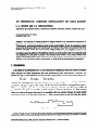
Abstract. The detection of timing problems in digital networks is of considerable importance. In
particular it is desirable to have efficient methods for discovering critical races and hazards.
Unfortunately, commercial simulators rarely provide such facilities; in fact, the simulators usually
assume that all the gate delays are exactly equal. In contrast to this, binary race analysis frequently
assumes that gate delays can be arbr;rarily large, though finite. An exception to this is the
almost-equal-delay race model, where gates have different delays, but the difference between any
two delays cannot be arbitrary. The difficulty with the use of this model is that it is computationally
very inefficient. In this paper we define a new ternary model which is very closely related to the
binary almost-equal-delay model. Moreover, the ternary model is considerably more efficient, as
efficient as the unit delay model; consequently, it could easily be incorporated in simulators.
1. Introduction
ted by examples; note that these examples
The ideas to be presented wi
were chosen for their simplicity and not necessarily their usefulness. Consider the
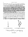
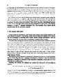
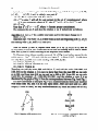
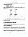
circuit of Fig. 1; the behavior of this circuit is governed by the following equations:
Y, = x’,
y2=xyt,
h=Y2+y3,
where, for each gate, yi denotes the present output of gate i and Yi, called the
excitation of gate i, gives the value of the boolean function computed by gate i.
When yi = Y;,,the gate has no tendency to change, and we say that it is stable. If
yi # Yi, then the gate is unstable and the output yi tries to change to Yi. This change
does not always happen because it is possible that an earlier change in some other
gate may cause Y;:to become equal to yi. This corresponds to the fact that the delay
Fig. 1. Network N, .
* This research was supported by the Natural Sciences and Engineering Research Council of Canada
under Grant A0871 and by a scholarship from the Institute for Computer Research, University of Waterloo.
0304-3975/88/$3.50
@ 1988, Elsevier Science Publishers B.V. (North-Holland)
50
C.-J.Seger, AA. Brzozowski
associated with gate i is inertial, in the sense that short periods of instability are
tolerated without any change. Now suppose the circuit of Fig. 1 is started with x = 0
and y=yl,y2,y3 = 1,0,0, which is a stable state. What happens when x is changed
to l? This is the type of problem that we are concerned with in this paper.
Any state in which more than one gate is unstable at the same time is called a
race. The outcome of a race depends very much on the model used. Commercial
simulators like SILOS [IO] or MOSSIM [Z] use the “unit-delay” (UD) model, in
which all gates are assumed to have exactly equal delays. In the state x = 1, y = 100
(commas omitted from 1, 0, 0 for simplicity) gates 1 and 2 are unstable, and will
both change. Consequently, the next state is 010. Now gates 2 and 3 are unstable,
and state 001 is reached. This state is stable. In summary, the unit-delay model
predicts that the final outcome of this transition is the stable state 001; see Fig. 2,
where unstable gates are indicated by underlining.
In contrast to this, the General Multiple Winner (GMW) model [7] permits the
possibility of unequal delays. The model assumes that any nonempty subset of the
set of unstable gates can change in any race. In Fig. 3 we show the GMW analysis
of network N1. If gate 1 is faster in state 100, the state 000 may be reached. This
is also a stable state, and represents a likely outcome. This shows that the UD model
is inaccurate. In fact, the only justification of the use of the UD model appears to
be its simplicity. On the other hand, the GMW model is too “pessimistic” as we
show below.
Consider the circuit of Fig. 4 started in the stable state x = 0, y = 1010100, and
let x change to 1. It is reasonable to assume that ys will change to 0 before y4
100
Fig. 2. Unit-delay analysis of network N, .
Fig. 3. Race analysis of NI according to the
GMW model.
Fig. 4. Network N,.
Optimistic ternary simulation of gate Mces
51
changes to 1, and that the only likely final outcome is the stable state 0101000.
However, the GMW model will allow the possibility that y4 changes before ys and
that the state OIOlOOlis also reachable.
The “almost-equal-delay” (AED) model, formally defined later, represents an
attempt to reduce the above pessimism by assuming that (roughly speaking) no gate
delay exceeds the sum of any two gate delays. Thus the AED model predicts only
the state 0101000 as the outcome for the circuit of Fig. 4 because the delay of gate
5 is assumed to be smaller than the sum of delays of gates 1,2,3 and 4. Note that
the AED model (extended to multiple winners) is clearly more informative than
the UD model since it always includes the outcome predicted by the UD model.
In this paper we define a new stepwise AED model and compare it with the
original AED model. We show that the two models are equivalent with respect to
their capability of predicting the outcome of a transition. However, the new stepwise
model has the attractive property of being closely related to a time scale; hence, it
is possible to obtain some timing information from the analysis.
A major difficulty with models such as the GMW and AED is that the number
of steps involved can be exponential in the number of gates. To overcome this,
ternary simulation has been used [l, 93 to perform the analysis more efficiently.
However, the ternary simulation algorithm, as suggested by Eichelberger [g], corresponds to a binary GMW analysis of the network assuming both gate and wire
delays [3,4], and is therefore even more pessimistic than the GMW analysis. To
overcome this, we propose a new ternary algorithm, called the ternary almost-equaldelay (TAED) model. This is a stepwise algorithm of the same complexity as the
UD method, but it takes into account possible races. In fact, we show that the
TAED model is closely related to the stepwise AED model.
2. The binary almost-equal-delay model
The “almost-equal-delay” (AED) model was originally defined using the “singlewinner” concept for simplicity [S, 61. In this paper we consider the more general
“multiple-winner” version of the model which is described below. This generalization
is quite straightforward.
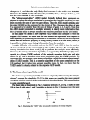
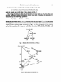
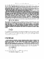
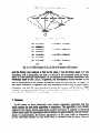
The basic idea is illustrated in Fig. 5. Suppose network A$ of Fig. 1 starts in state
100 at time 0 with gates 1 and 2 unstable as shown in Fig. 5. Suppose now that gate
(a)
W
Fig. 5. Illustrating the “AED” idea: (a) possible transition; (b) timing diagram.
C.-J. Seger, J.A. Brzozowski
52
2 wins the race at time t and that, as a result of that change in gate 2, gate 3 becomes
unstable. Under the almost-equal-delay assumption, it is unreasonable to let gate 3
win the new race between gates 1 and 3 since ;&e 1 has already been “waiting”
for t units of time. The model will remember this fact and will only permit gate 1
to change in state 110, predicting the next state as 010. Informally, we can consider
that at time 0 a “race unit” has started involving gates 1 and 2. No other gate can
“enter” this race unit until all the gates in the original unit are somehow “satisfied”.
A gate becomes satisfied if it either changes or becomes stable as a result of some
other change. These ideas will be made precise below.
Consider a network with n gates whose outputs are given by the vector y=
!:I,. . . , y,, and with m inputs given by x = x1, . . . , x,. With each gate yi we associate
its boolean function Yi(q y). In the AED model a certain amount of previous race
history is necessary to determine the outcome of a race. We therefore define a race
state to be an ordered pair (y, S), where y E B” denotes a state of the network, and
S denotes the set of gates that are unstable in that state and are candidates to change
according to the AED model, as explained below.
Given any gate state y = y, , . . . , y”, and any subset P of the set (1,. . . , n} of gate
subscripts, we define ytP) to be the vector obtained from y by complementing all
the yi such that i is in I? For example, if y = 100 and P = (1,3}, then y(‘) =OOl.
We now define a set K of race states and a binary relation p on K We begin
with a stable state X, y”, and change the input to Z The initial race state of the
network is (y’, U(y’)), where, for any y, U(y) is the set of subscripts of unstable
gates in state y, i.e.,
(Note that the input will be held constant at the value x’ for the rest of the analysis;
thus the dependency of U on x”is suppressed.)
The set K and the relation p are now defined inductively as follows:
Basis: (y”, U(YO))EK
Induction Step: Given (y, V) E K,
(I) if V=0, then (y, V)p(y, W;
(2) if V# 0, then for each nonempty subset P of V compute WP= ( V- P) n
U(fP’);
(a) if Wp=fl, then (y (p), wY’p’)k
(p) u(y’p’)).
K and (Y, VP(Y
(b) if W” #0, then (y (‘I, Wp) E K and (y, V)p(y’p), Wi).
Nothing else is in K or p.
The set
defined above represents the set of all possible race states reachable
from the initial race state (y’, U(y’)), and the relation p describes the immediate
successor race states. In particular, given (y, V), if V= 0, then y is a stable state,
and this is indicated by stating that (y, 0) is the only successor of itself. Next, if
is definition that V will always represent a subset of the
Optimistic ternary simulation of gate mces
53
state y(‘) may be reached. The gates in are considered to have completed the
race they were involved in. As for the gates in V- P, one of two things can happen.
Either a gate yi remains unstable in ytP’, i.e., ie Wp, or the instability of yi is
removed when y changes to y (‘I . In the latter case, ie W,. Now, if
=p), al1 the
instabilities have been remo
from V, one way or another. Thus we consider the
previous race unit as compl
, and now start a new one by entering the race state
(y(‘), U(y(“))) where each unstable gate of y (‘I has an equal chance of winning. If
W, # 0, then some of the instabilities of V still remain unsatisfied; these a
all the gates in Wp These gates are given preference over any new instabilities that
may have been introduced by the change from y to y?
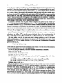
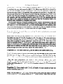
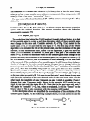
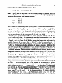
We illustrate this definition by the following example. Consider the network N,
of Fig. 1 in state x = 0, y”= 100 which is stable. We now let x’= 1 and note that
U(y’) = {1,2}. Thus the network starts in the race state (100, {1,2}). The graph of
the relation p is shown in Fig. 6, where each edge has a label showing the gates
that change during the transition corresponding to the edge. (For now, ignore the
*-marking on some edges.)
The relation graph shown in Fig. 6 describes all the possible states that can be
reached during the transition from the initial state y” = 100, when the input changes
from 0 to 1. However, we are normally interested only in the “final” outcome of
the transition. Thus we will consider only the set of cycles in the relation graph of
so
Fig. 6. Race analysis of N, according to the AED method.
54
C.-J.Seger, J.A.
Brzozowski
p. Note that, by the definition of p, there cannot be any transi
(A cycle is said to be transient if there is a gate that has
unstable in all the states of the cycle [7].) In this case the netwo
either one of two possible cycles, namely the stable states 000
initial race is critical because the final outcome depends on th
the circuit.
For technical reasons which will become clearer later, we mark certain edges by
a * in the graph of p as follows. All edges of the type ((y, a), (y, 0)) are marked.
Also, every edge ((Y, V), (Yw 9 U(Y’~‘))) added to p by rule (2)(a), i.e. with W, = 0,
is marked. No other edges are marked. (Note that if an edge is introduced because
of rule (2)(a), that same edge cannot be also generated by rule (2)(b). This follows
because y, V, and y(‘) uniquely determine W,.) For example, Fig. 6 shows all the
marked edges for the previous example.
In this section we introduce a new binary race model, very closely related to the
AED model of Section 2. This model, which will be called the stepwise AED model,
has the advantage of showing more clearly certain timing information. Also the
stepwise model will be used later to establish a related ternary model.
To obtain more timing information from p we now define a new relation R derived
from p as described below. Intuitively, one can interpret this relation R in the
following way. Suppose that all the gates have approximately the same delay, 6 f E.
Then any race unit lasts for approximately 6 units of time. Thus a transition between
two distinct states related by R represents roughly -8 units of time. In contrast to
this, consider the relation p of Fig. 6 and the sequence (100, { 1,2}), (110, {l}),
(010, {2,3}) where consecutive race states are related by p. Here the first transition
takes about 8 units of time, whereas the second one takes only E units of time,
because gate 1 became unstable in the first state and lagged behind gate 2 by a
small amount of time.
Note that the a ove intuitive explanation is adequate as long as 6 is much smaller
than 6. Note als that the *-marking introduced in Section 2 has the following
meaning: a transition is marked iff that transition completes a race unit, or it is a
self-loop on a stable stat
Formally, the relation is defined on a subset Q of the set K of race states as
follows:
Q = {(y”, U(y’))} u {(y, V) : there is a marked edge into
(y, V) in the graph of p}.
Optimistic ternary simulation of gate races
55
To illustrate this, consider the example of Fig. 6. We find
Q = WR U,2h WO, f&3)), (000, @, (OOI,0k
and the reader can verify that R is as shown in Fig. 7.
The reader should note that the knowledge of a race state (y, V) alone does not
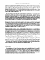
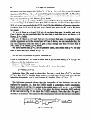
provide sufficient timing information about race units. Consider the network AT’
described by the following equations:
Y, =xy$,
Y*=Js,
&=Y2
started in the stable state x = 0, y = 000 and with the new input x^= 1. (We use some
strange gates in this network in order to keep the example small; similar phenomena
occur in more realistic larger circuits.) In Fig. 8 we show the graph of the relation
p for this transition. It is easy to verify that the states (000, {1,2}), (010, {3}),and
Fig. 7. Relation R derived from p of Fig. 6.
Fig. 8. AED analysis of network I$.
56
C.-J.Seger, J.A. Brzozowski
(110, {1,3}) are all in Q, and that (000, {1,2})R(OlO, (3)) because the change in gate
2 completes the race unit started in (000, { 1,2}). When state (010, (3)) is reached in
this way the instability of gate 3 represents a new race unit. owever, despite the
fact that the states (110, { 1,3}) and (010, (3)) are both in Q and (110, { ,3})p(OlO, {3}),
they are not related by R The reason for this is that the transition from (110, { 1,3})
to (010, {3}) does not represent the completion of a “race unit”, because gate 3 is
still unstable, and that condition started in state (110, { 1,‘3}). By requiring that the
last edge in the p-path be marked, we make sure that the R-relation holds c~rlly
between states reachable by complete race units.
We will show that the I? relation contains all the “useful” information of the old
AED relation p. Assume the network is started in the stable state X, y” and that the
new input is 2 For convenience, let GP be the directed graph of the relation p, and
GR be the directed graph of the relation R Note that GP and GR depend not only
on the network, but also on +he initial state and the input change.
Proposition 3J. In the grape GR every node (y, V) E Q is reachable from the initial
race state Go, U(yO)).
Proof. First note that, by the definition of p, all nodes in GP are reachable from
the initial race state (y’, U(y’)). Consider (y, V) E Q; either (y, V) is the initial state
or it has a marked edge (@, v), (x V)) in GP into it. Obviously, if it is the initial
state, there is nothing to prove. Otherwise, study the state (y, v). Note that (9, v)
must be reachable from (y’, U(y’)) in GP, and hence there must exist a path in GP
from (y’, U(y’)) to (y, V) ending with a marked edge. In this path some other edges
might also be marked, but that will only mean that we can reach (y, V) in GR by
going through more than one node. Hence the claim follows. Cl
position 3.2. TOlestable states of GP are the same as the stable states of GR.
Proof. All stable states of GP are of the form (y, 0}, with an edge ((y, 0), (y, 0)). Note
that this type of edge in GP is always marked and hence will also exist in GR.
Conversely, every stable state of GR is a stable state of GP by construction of R 0
For the next proposition we need a new concept. Given any cycle
(Y’s V’) , . . . , (y’, V’), (y*, V’) in the graph GPIwe call a race state (y’, Vi) initiating
in this cycle iff the edge ((yi-‘, Vi-‘), (yi, Vi,\) is marked, where (y’, V”) is interpreted
as (yr, V’).
33. Every simple cycle C in G,, of length 32 must contain at least two
distinct initiating states in C.
such a cycle, eith
i-’ (Case (2)(b))
edge is marked
from any race
Optimistic ternary simulationof gate races
57
state in C we must reach an initiating state in C in a finite number of steps. Starting
from any initiating state (y, V) in C we eventually must reach another initiating
state (9, V) in C. We argue that these two race states must be different. This is
because the edge leaving (y, V) involves changing at least one variable, say yi, from
V. This variable cannot change again until a new initiating state in C is reached.
Thus y^and y differ at least in yi. 0
We now wish to show that the cyclic behavior predicted by p is in some sense
preserved in R For any cycle C of race states in the graph G,,, let n(C) be the
sequence of initiating states of C in the same order as in C. The AED model of
Section 2 (relation p) and the stepwise model of this section (relation R) are related
by the following result. Assume that the network is started in the stable state x, y”
and the input changes to 2. Compute p and R starting from this condition.
Theorem 3.4. For every cycle C in the graph G,, there exists a cycle lI( C) in the graph
GR. Conversely,for every cycle D in GR there exists a cycle C in GPsuch that D = I?(C).
Furthermore,given two corresponding cycles CP in GP and CR in GR, and any variable
yi, either yi has the same binary value in all the states of Cp and CR or yi oscillates
(assumes the values 0 and 1) in both CP and Cp.
Proof. Consider a cycle C,.,in G,,. If the length of the cycle is I, i.e., the state is a
stable state, then the result follows immediately from Proposition 3.2. Hence, assume
the length of the cycle is 22. By the definition of an initiating state in a cycle and
the definition of n(CP), it follows that if (y, V) and (9, 9) are any two consecutive
race states in n(C,,), then the path in CP from (y, V) to (j7, V) will have only the
last edge marked. Therefore we can conclude that (y, V)R(y, V). This, together with
Proposition 3.3 shows that n(C,,) is a cycle in GR of length 32.
Conversely, let DR be a cycle of GR. According to the definition of R, for any
two consecutive race states (y, V) and (9, V) in DR, there must exist a path in the
graph G,, from (y, V) to (y, V) with only the last edge marked. Hence there must
exist in GP a cycle CP corresponding to the cycle DR in GR such that n( C,) = DRThe final part of Theorem 3.4 follows immediately from the observation that a
gate can change at most once between two initiating states. Cl
4. Race units
The definition of Q and R as given above can be simplified since it is possible
to avoid using race states. This follows because, in any state (y, V) in Q, the set V
is uniquely determined by y ( V = U(y)). Below we give a different algorithm for
of p. e reader
computing Q and R, where we do not explicitly form the g
ition.
can easily verify that the result is equivalent to the previous
C.-l. Seger, I.A. Brzozowski
58
As before, we consider a gate network defined by X,y, and Y. A sequence, ( zO,So),
(z’, S’), . . . , (z’, S’), k 2 0, is called a race unit if
(i) z” E B” is a gate state and So =
ii z’+’ is state z’ with all the gate outputs in the set A’ co
emented, where
( )
zi+*), and
A’ is any nonempty subset of S’; also Sif’ = (Si (iii) Sk = 0.
=>Sk, where =>denotes proper containment.
Note that S”D S’ =)
We compute the set 2 and also the relation o on 2 inductively as follows:
l
l
l
Algorithm 4.1. Let X, y” be a stable total state and let the input change to %
Basis: y%Z
Induction step: For every y E 2, if there exists a race unit beginning wit
and ending with (z, @),then z E Z and yoz.
Now to obtain Q and R, replace each state y E 2! by (y, U(y)) in Q and let
(Y, WY)uWli
WI)
iflEY OZ. From now on we will be working with 2 and 0 rather
than with Q and R when referring to the stepwise AED model.
To illustrate these ideas, consider network N, of Fig. 1, as before started in the
stable state x = 0, y” = 100 and with the new input x’= 1. Since U(y’) = { 1,2}, there
are only three possible race units starting with (100, { 1,2}):
(1) (IOO,U, 2Mm, 01,
(2) WA {1,2HWO, W~(O10,0), and
(3) (100,{1,2H(OIO,
0).
Therefore we add the states 000 and 010 to 2, and add the pairs (100,000) and
(100,010) to the relation a. It is easy to show that from the state 000 we can only
go to 000, and from state 010 we can end up in 000 or 001. From 001 we can only
reach 001. In summary, 2 = {100,000,010, OOl}, and the relation m over 2 is as
illustrated by the graph of Fig. 9. Note the correspondence between Fig. 9 and Fig. 7.
It is now convenient to interpret Fig. 9 as a nondeterministic finite-state machine
with initial state 100, and S as its only input letter. After one race unit (i.e., after
roughly S units of time), we may nondeterministic:dslyreach the states 000 or 010,
1
100
(100)
1
0
(000.010)
1
000
001
Fig. 9. Stepwise AED analysis of N, .
c00
Fig. !O. 6hrrqmRSng
kteministic
machine ;o Fig. 9.
finite-state
Optimisticternary simulation of gate races
59
etc. Let Z”= {y’} and let 2’ be the set of states of
reachable after i steps, i.e.,
Zi = {z : y’o’z). Note that these sets are the same as the subsets constructed by the
subset construction when converting the nondeterministic finite state
deterministic finite state machine. In Fig. 10 we show the deterministic finite-state
machine corresponding to the non
erministic machine of Fig. 9.
We close this section with a discus&it of some limitations of the stepwise A
model. One of the basic assumptions in this model is that delays are only associated
with gates, and that delays are inertial in their nature. In many re
mptions can be well justified. However, there is also a danger that the model
may become unrealistic under certain conditions. ‘The model is only accurate as
long as races from different race units do not get “mixed up”. In general, under
the assumption that all gates have delays Ai in the interval [ 6 - E, S + c], the following
condition makes sure that the kth race unit does not get mixed up with the (k - 1)st:
k(S-s)>(k-l)@+s).
The condition states that the time to complete k changes in the fastest gates (each
with delay 6 - E) should be greater than the time required for k - 1 slowest gates
(each with delay 6 + 8). What can happen, if the above condition is not satisfied,
is that the model may omit certain races that potentially could exist.
a sufficient condition for the stepwise AED model to be accurate for at least k steps,
is that
z<- 1
6 2k-1’
For example, if the uncertainty of the delays in the gates is lo%, the stepwise AED
model is accurate for at least five steps. However, the reader should note that the
above condition is only a sufficient condition; in many cases the AED model is
accurate for more than k steps.
5. The TAED mdel
In this section we describe a ternary simulation method which is related to the
stepwise AED model. For more details about ternary simulation in general, the
reader should refer to [T]. Let T = (0,1,$}. The values 0 and 1 represent the usual
logic levels and i represents an unknown value. We will use the following convention.
= (0, l), will have corresponding
Variables like yi etc., which take values from
variable:; yi etc. taking values from T The partial order s on T is defined by
rat
forall tE T,
0 < 5!
and
1s;.
V4e extend the partial order s to T” in the usual way:
tSt
iff fiGPi
foralli=l,...,m.
The statement TVc means that whenever ri is
value as ri, but c may contain more unknown
value 4). Thus r has more **uncertainty”
For any vector of boolean functions f:
defined by
f(r)=lub(f(a):aEB’and
a+.
It follows that, for t E B’, f(f) = f( t)
agrees with the ori
monotonicity property [7]:
t< I implies
f(t)e
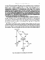
The underlying idea behind the TAED method, formally de ed below, is to
ne which of these unstable gates
all the unstable gates in a state y9and then d
must change in this race unit. Consider ne
N4 of Fig. II(a) started in the
stable state x = 0, y = 11 and with the new input x”= 1. The first step of the TAED
algorithm is to calculate the lub of the
ent state, and the excitation of
network. In this interm
t iq the algorithm, a
value 5 if it is unstable. In network
both gate 1 and gate 2 are unstable and
hence t = if. In order to determine
f the unstable gates must change in the
present race unit, the excitations of the unstable gates (i.e., the gates for which 9 = f)
are re-evaluated. However, this re-evaluation is done assuming t is the total state
of the network. If the excitation of an unstable gate j is still binary, then, independently of changes in the other unstable gates, this gate has to change before the
present race unit can finish. On the other hand, if the “new” excitation of an unstable
gate j is i, then that instability “depends” on some gates that are also unstable.
Wence it is possible to change these other
table gates first and thereby remove
the instability of gatej. In network N’ we get
l,#=
l’=Oand Y,(l,$f)=(lf)‘=~,
so the new state we reach is O&It is easy to see that gate 1 must change in any race
unit since the excitation of the gate depends only on the new input value. an the
other hand, the instability of gate 2 depends on gate 1 which is unstable; if gate 1
changes first, gate 2 becomes stable. Hence in the step
AED model we can
reach in one race unit the states 00 or 01. Note that in
in be “unstable” (=f), but, when re-evaluated,
binary value 0. This is also consistent with the stepwise AED model.
In the description above we simplified the re-evaluation of the excitation of the
unstable gates slightly. As the following example shows, it is not correct to use the
(b)
Fig. 11. (a) Network
TAED method.
We define the function
be any ternary
state.
-first calculate the intermediate st
5 = lub(y,, q(g Y))
1
forj=l
{
to n do
-re-evaluate the excitation
The TAED algorithm consists of repeatedly appfyin next* Note that this wilf
either lead to a stable ternary state, or an oscillation. n this respect the TAED
method is similar to the unit-delay method used by most commercial simulators.
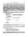
To illustrate the algorithm, consider network Nt of
stafled in the st&Jle
state x = 0, y” = 100 and with the new input Z = I. The fi
the following intermediate values: ?
(:, y”)} = iub{ t, -r’}= lub{ 1,Q) = f ,
(?, y”)} = lub(O,(Zy;,, = I
Hence, t = f@. In the second step of
state are re-evaluated using the inte
5
C.-J. Seger, J.A Brrozowski
62
itself for which we use the “old” vs!ue. For network IV, we re-evaluate gates 1 and
2, and we get the following values:
j71t y& t(‘)) = #”= 0,
$2 = Y& #(*I)= (3,) = (19) = $.
Hence, we obtain the new state 5 = [email protected] Fig. 12(a) we give the complete TAED
analysis of network N,.
I0 *
y*= _loo
I
I
?'=&a0
I
y’= Oh0
c
{too)
z’s {ooo.010)
ta=Ok%
I
y== 00%
0
(a)
z”
I
@oo.
001)
0
(b)
Fig. 12. Analysis of IV,: (a) TAED model; (b) states reachable in stepwise AED model.
It is interesting to note that the lub of the states reachable after i race units in
the stepwise AED model corresponds exactly to the outcome of the TAED method
after i steps; see Fig. 12(a) and (b). In the next section we explore the relationship
between the two models.
6. A partial characterization of the TAED method
In this section we show a partial correspondence between the binary stepwise
AED model and the results of the TAED algorithm described above. The main
result is the following theorem.
mre.rn~
6.1. Let x, y* be a stable total state, and let x’denote a new input uector. Let
yi denote the results of the TAED method after ib0 steps starting in y*= y*. Then,
yi 2 lub(Z’), whereZ’ is the set of states reachable in i steps in the stepwise AED model.
efore proving the theorem we will establish Lemma 6.2 below. The following
servation is useful in proving the lemma. If y is the input to ext, then t(j) > y.
ence, by the monotonicity property of the ternary extension,
0)
Optimistic ternary simulation of gate races
.2. Let YE T” and let 3 be
w <y
and
63
t(y). 7hen
wuz implies z s 5.
Proof. If j;i = 4, then for any such z we will trivially have fi a 3. Hence, study the
cases when fi E D. Note that, by the definition of G it follows that ~3= 4 implies 5 = f .
Therefore there are only four cases to consider.
1234
Yj=
p
(II
Yj =
bbbi
b” 2
2
d
b b b’ b
Here b stands for some binary value (0 or I), and b’ denotes the complement of b.
Case 1: a = b, 5 = b, and jii = b. By the definition of 4,~ = b implies that
b. Furthermore, by the definition of ternary extension, we must also have yi($ w) = b
for every w 6 y. Since Wj S yi = b, gate j is stable in any such state w. Consequently,
gate j remains unchanged in any race sequence beginning in state w. Therefore, if
waz, we must have 3 = 6. By assumption, jii = b and fi > z; holds.
&se 2: yi=b, ti=f, and j$=b. If $=
n q(gy) is either $ or 6’. By (l),
I$(% t(j))2 Y,(g y). Thus 6, as computed
, must have the value 3 or b’. But
we have assumed ii, = b. Hence this case is impossible.
Case 3: y,=b, $=$, and&= b’. We first prove that, in any state w G y, gate j is
unstable. Since $ = $, we know that fi = Yj(Z, t(j)). Also, by assumption, fi = b’.
Altogether we have Y# t(j)) = b’. By (l), we know that q(g t(j))2 q(g y), so
b’= q(g y). Furthermore, by the definition of ternary extension, it follows that
q($ w) 6 q(<y) when w by. Hence b’= ts_(S,w) for w my. Since w by, andyi = b,
we must have wj = b. Together, this shows that gate j is unstable in any state w s y.
Secondly, we show that for any race sequence starting in state w, gate j must
change, and therefore, for any z such that wmz, we will have Zj= b’. We prove this
by contradiction. Assume there exists a race sequence (z’, So), (z’, S’), . . . , (z”, Sk)
(ka0) with z”= w, So= U(w), and Sk = 0, such that z; = 6. Since, according to the
first part above, gate j is unstable in any state w 6 y, we can conclude that k 2 1.
Furthermore, since w s y, and, by assumption, fi = b, we must have zy = h
by the definition of a race sequence, it follows that a gate can change at
during a race sequence; since zy - b and z; is assumed to be b, it follows
for p=O,..., k Since t = lub(y, (2,y)), it follows by the definition of ternary
eT;:Gnsionthat t 3 lub( w, Y( 2, w)) for w < y. Furthermore, by the definition of a race
Ianit, it follows that for j = 1, . . . , n, and p = 0, . . . , k, we have that zipis either equal
to Wjor q(?, w). We can therefore c
ub(w, Y(% w)), and hen
t2zp
:orp=O,...,
shows that t(j)3zp
for p=O,...,
Z,zp) for p=O,...
C.-J.Seger, JA
64
Btzozowski
the above two facts imply that yi(s, z p, = b’ for p = 0, . .
that j is in U(zp) forp = 0, - , k contradicting the assum
the assumption must have been false, and we can con
that w(rz must have 3 = b’. Hence, fi 2 3 holds.
Since 5 = f , it follows that
case& a=#,%=$,andj?i
sumed iij = b, it follows
q(Js, t(j)) = b. By (l),
5, y), so we can conclude th &(g y) = b. By the definition of ternary extension,
ows that x(5, w) = b for any w s y. Study any state w E B”, w G y. We have
l
l
0i wj = b. Since wj = b and U,(?, w) = b, we have that gate j is stable, and, as in
Case 1 above, we can conclude that, for any state z such that woz, we have zj = b.
Hence, ij 2 3 holds.
(ii) wj = b’. Since wj= b’ and q(g w) = b, we have that gate j is unstable. Using
similar arguments as in the second part of Case 3 above, we can conclude that, for
any race sequence from the state w, gate j must change and thus we have that if
WOZ, then zj = b. Hence, jii 3 zj holds.
We have shown that iiJ
r all possible cases, and hence that y’2 z for any
state z, such that woz, where
We are now in position to prove Theorem 6.1.
of
eorellh6.1. We want to show that if J$ E B, then lub(zj : y”
will prove this by induction on i
Basis: i = 0. Trivially true.
Induction Hypothesis: Assume that, for all k G & we have that
a’~}
= J$.
We
Induction Step: We need to show that, for any z such that ~‘u’~‘z, we have
implies there exists a w such that y’a’w and woz. By the
induction hypothesis, w G yi, and Lemma 6.2 applies. Thus, y’+’ a z. Cl
Y i+l az. But yooi+’ z
e following example shows that the inequality of the theorem can not be
replaced by equality, i.e., that the TAED model is sometimes overly pessimistic.
Study network J’+&
of Fig. 13, started in the stable state x = 0, y = yi . . . y6 = 111000
and with the new input x’= 1. In Fig. 14 we show the binary stepwise AED analysis
of the face and in Fig. 15 we show the TAED analysis. Note that the f for gate 5
in state y2 is incorrect. The reason for this discrepancy between the ternary simulation
Optimisticternary simdation of gate races
65
Fig. 14. Stepwise AED analysis of N6.
l.u.b.(Z”) = 111000
1.u.b.Q’) = Ol%OOO
I.u.b.(Z”) = 010000
w
(b)
Fig. 15. (a) TAED analysis of N,; (b) Iub of the stepwise AED analysis.
and the binary race analysis is that in the state y’ not all binary states by’ are
reachable, and in particular, the state y = 011100 is not reachable from the initial
state. It is this state that causes gate 5 to be unstable in the ternary simulation. and
eventually leads to the 4 in yg. In general, the discrepancy occurs because of the
loss of information in the ternary simulation where we only use the “average” of
the states reachable. It appears that this pessimism occurs only in pathological
examples, and that for most practical circuits, the ternary and the binary AED
analysis correspond exactly. However, the problem of characteriing the class of
networks for which the two models agree remains open.
7. Summary
In this paper we have presented a new ternary simulation algorithm that can
easily replace the unit-delay algorithm in simulators. The algorithm is very closely
related to the binary almost-equal-delay model, a
ce is capable of detectin
critical races under the assumption that all delays are a
CT.4 Seger, J.A. Brzozowski
66
evaluations). A major disadvantage with both this ternary algorithm and with the
unit-delay method is that the algorithms are not guaranteed to h
test whether a ternary stable state is reached by comparing y a
is binary, we know the circuit reliably reaches a unique stable st
critical race or an oscillation is likely, and further analysis is required. Since there
are at most 3” reachable ternary states, it is decidable whether the analysis predicts
binary stable state. However, for large networks this decision may involve
a unit
an excessive amount of computation. For such reasons commercial simulatars simply
terminate the computation when the number of steps exceeds some arbitrarilychosen
relatively small limit. The same approach can be used here. One can argue that a
practical circuit that does not stabilize in (say) ten race units is not very well designed.
Consequently, the method can be made practical and should produce useful results.
eferences
R.E. Bryant, Race detection in MOS circuits by ternary simulation, in: F. Anceau and E.J. Aas,
eds., VLSI ‘83 (Elsevier Science Publishers B.V., Amsterdam, 1983) 85-95.
R.E. Bryant, A switch-level model and simulator for MOS digital systems, IEEE Trans. Comput.
C-33(2) (1984) 160-177.
J.A. Btzozowski and C.-J. Seger, A characterization of ternary simulation of gate networks, IEEE
Trans. Comput. C-36(11) (1987) 1318-1327.
J.A. BROZOW& and C.-J. Seger, Correspondence between ternary simulation and binary race
analysis in gate networks, in: G. Goos and 1. Hartmanis, eds., Lecture Notes in Computer Science
226 (Springer, Berlin, 1986) 69-78.
LA. Btzozowski and M. Yoeli, Models for analysis of races in sequential networks, in: A. Blikle,
ed., Lecture Notes in Computer Science 28 (Springer, Berlin, 1975) 26-32.
LA. Brzozowski and M. Yoeli, Digital Networks (Prentice-Hall, Englewood Cliffs, NJ, 1976).
J.A. BROZOWS~~
and M. Yoeli, On a ternary model of gate networks, IEEE Tmns. Compui C-28(3)
(1979) 178-183.
E-B. Eichelberger, Hazard detection in combinational and sequential switching circuits, Ii3&f 1.
Res. Dewlop. 9 (1965) 90-99.
J.S. Jephson, R.P. McQuarrie and R.E. Vogelsberg, A three-level design verification system, IBM
Systems J.8(3) (1969) 178488.
SimuTec, SILOS: Logic Simulator User’s Manual.