Download Pasco Xplorer GLX - The Gaia Project

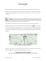
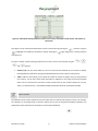
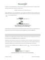
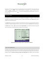
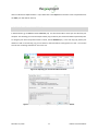
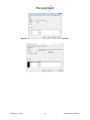
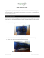
XPLORER GLX
This guide covers the major features of this product - it does not cover all of the available functions. This guide is
not intended to replace the original equipment manual. Please refer to the manual for more detailed operating
instructions and safety information.
EQUIPMENT DESCRIPTION
The Xplorer GLX is a portable data logging device, with a graphical user interface making it ideal for use by
students. Data can be later exported and analyzed on a computer. It is capable of accepting and using a variety of
different sensors, including:

Up to four sensors using the ports on the top of the device [1]
Figure 1: Four Sensor Ports on top of GLX

Up to two additional temperature sensors, using the ports on the left hand side of the screen [2]

A voltage sensor using the port on the left hand side of the screen [2]
Figure 2: Two Temperature Ports and Voltage Port on side of GLX
December 21, 2010
1
realistic environmentalism

A built-in microphone is available for use as a sound sensor
This guide is designed to cover the majority of functions that you will probably use on a regular basis. It is not
comprehensive, and you may need to refer to the original user manual for more detailed instructions or for more
specific applications.
OPERATION
POWER
The Xplorer GLX has a rechargeable battery allowing it to be used portably. The GLX can be turned on by pressing
and holding the
the
button in the bottom right corner of the device. The GLX can be turned off again by holding
button.
In order to charge the battery, the AC adaptor must be plugged into the power port on the right hand side of the
GLX [3]. When plugged in, the GLX will automatically turn on and cannot be shut down.
In order to preserve the battery, it is recommended that the GLX be plugged in whenever possible.
Figure 3: Power Port on side of GLX
NAVIGATION
To navigate around the menus on the GLX, simply use the
December 21, 2010
2
to move, and the
to select.
realistic environmentalism
COMPUTER CONNECTION
The Xplorer GLX can be connected to a computer using the USB port on the side of the GLX [3] near the power
port. The software interfaces with the Pasco DataStudio, which can be used in place of most of the functions
described in this manual. While we have included a Quick Start Guide for DataStudio, it may not be licensed at
your school, in which case you can choose to export data as a text file to manipulate it in Microsoft Excel, which is
described at the end of this guide in the section EXPORTING DATA
HOME SCREEN
The Home screen [4] can be reached at any time by pressing the
button located underneath the directional
arrows.
Figure 4: Home Screen
This screen allows you to configure options, and select which mode to view data.
SETTINGS
The Settings menu allows you to set a number of different settings including:





Date and Time
Date and Time Format
Device Name
Auto Power Off Settings
Backlight and Contrast Settings
December 21, 2010
3
realistic environmentalism
Contrast can be adjusted at any point by holding down the
button and using the
arrows.
Data Files
Before collecting any new data you should create a new file. After entering the Data Files mode, you’ll be
presented with the following screen [5].
Figure 5: Data Files Mode
To create a new file, simply press
and select New File. A new file will be created with the name Untitled,
and will be highlighted. To change the name of the file, press the
Pad to enter a new file name (just like texting). Press the
, and use the
button and the Number
again to confirm the name.
This menu can also be used to:





Open files
Save files
Delete files
Save As
Rename files
SENSORS
Entering Sensor mode [6] will allow you to configure the sensors.
December 21, 2010
4
realistic environmentalism
Figure 6: Sensor Mode
Each sensor connected will be listed along the top of the screen, with a small icon identifying the type of sensor
and a number above it indicating the sensor number. You can see that there are two sensors connected in Figure
6. You can switch between which sensor you are configuring by using the
For each sensor you can configure (using the

arrows, and the
arrows.
):
Sample Rate Unit: Combined with the Sample Rate below, this allows you to configure how often the GLX
reads the value from the sensor. You can choose to read the sensor a certain number of times per second
(samples/s), or every certain number of seconds, minutes or hours.

Sample Rate: Here you can choose the value to associate with the Sample Rate Unit. For example,
selecting 5 here, and samples/s in Sample Rate Unit would have the GLX read the sensor value 5 times a
second. Changing Sample Rate Unit to seconds would result in the GLX reading the sensor value every 5
seconds.

Reduce / Smooth Averaging: This allows you to smooth out the data points by averaging a certain
number of points. A larger value will give you a smoother curve, but you’ll miss quick changes in the data
values. The impact of averaging is shown in Figure [7].
Figure 7: Averaging

Visible / Not Visible: You can choose to make a sensor invisible without disconnecting it.
December 21, 2010
5
realistic environmentalism
It is highly recommended that you select the same Sample Rate Unit and Sample Rate for all connected sensors.
Remember that a faster Sample Rate will reduce the length of time that the GLX can collect data for before filling
its memory. Recording lighting levels in a room every second may not be necessary – once a minute may be more
than adequate.
GRAPH
Entering the graph mode [8] will allow you to begin and view data collection.
Initially, the graph will be displayed with one sensor on the vertical (Y) axis, and time on the horizontal (X) axis.
Pressing the
will allow the user to change the way the data is plotted. Using the
the title on any axis and press the
keys, you can select
again to change which sensor is plotted on that axis (depending on whether
or not sensors are connected). By selecting the units, you can choose the units in which the data is plotted (for
example temperature could be in ºC, ºF or K). You can also select which Run to plot if more than one run has been
conducted.
Figure 8: Graph Mode indicating how to change fields
Pressing the
change from a
button will commence data acquisition, and the icon in the top right of the screen [9] will
icon to a
icon indicating that data collection is in process.
Figure 10: Top bar showing that data acquisition is not currently active (third icon from right)
December 21, 2010
6
realistic environmentalism
Pressing
again will cease data acquisition. Every time you start the data acquisition again, the data
collected will be stored in a new Run. The Run number can be seen in the top right hand corner of the screen.
You have a number of options along the bottom of the screen, which can be selected using the
and

,
,
buttons
Auto Scale: The scale of the graph will be automatically adjusted to show an appropriate vertical range
that fits all of the data collected. The scale will automatically adjust as the data is collected.

Scale / Move: Pressing this button will alternate you between Scale and Move mode. In Scale mode, you
can scale the vertical axis with the
arrows and the horizontal axis with the
arrows. In Move
mode, you can move the scales using the same procedure. After about 10 seconds of no activity, the GLX
will exit both modes.

Tools: The tools menu will allow you to select a number of data analysis tools. These include tools that
will allow you to determine the slope of the graph at any particular point, as well as add a straight line of
best fit to a set of data points. These are more advanced functions, and reference should be made to the
user manual for details.

Graphs
o
Two Measurements: Selecting this mode allows you to view the data from two sensors
simultaneously on the same graph. You can choose which sensors to plot using method
described previously.
o
Two Runs: Selecting this mode will allow you to view the data from one run against the data
from a second run. You can choose which runs to plot using method described previously.
o
Two Graphs: Selecting this mode allows you to view the data from two sensors simultaneously
on different graphs. You can choose which sensors to plot using method described previously.
TABLE
The functionality of the Table mode [10] is very similar to the Graph mode, but instead allows you to see the data
in table format.
December 21, 2010
7
realistic environmentalism
Figure 10: Table Mode showing temperature data in one column, and a blank second column, and statistics at
the bottom
Once again you can choose which information to show in each column by pressing the
to highlight the variable you would like to change. Pressing the
, and then using the
again will give you a variety of options
to choose from.
You have a number of options along the bottom of the screen, which can be selected using the
and

,
.
buttons.
Statistics [10] – F1: This menu allows you to see a variety of basic statistics for each column on display
including Maximum, Minimum, Average, Standard Deviation and Count (number of data points).

Tables – F4: This menu allows you to choose the number of columns to display. Once you have selected
new columns, you can then choose what information is displayed in them using the process described
above. You can also choose to show time in either seconds since the start of data collection (i.e. 0s, 60s,
120s), or in absolute time (i.e. 25/12/2010 13:00:00, 25/12/2010 13:01:00, 25/12/2010 13:02:00).
CALCULATOR
The calculator can be used to calculate and record a value that isn’t directly measured by the sensor. For example,
the calculator can be programmed to allow the Xplorer GLX to plot the temperature difference between two
temperature probes instead of the temperature of each probe individually.
December 21, 2010
8
realistic environmentalism
To perform a sensor based calculation, connect the necessary sensors, and push the button to collect some data.
Open the calculator mode, and enter your formula, such as:
TempDiff = [Temperature 1 (°C)] - [Temperature 2 (°C)]
Where [Temperature 1 (°C)] and [Temperature 2 (°C)] represent two temperature sensors connected to the
Xplorer GLX. Instead of typing [Temperature 1 (°C)] and [Temperature 2 (°C)], you can select each one by pressing
to enter the data menu [11].
Figure 11: Selecting Sensors in Calculator Mode
When collecting data using the Xplorer GLX, the GLX will automatically calculate and store the equations entered in
Calculator Mode. They will also be available to be plotted in Graph mode, and viewed in Table mode.
MANUAL / CONTINUOUS
By default, the GLX collects data in continuous mode. This means that it takes a reading from the sensor in
intervals according to the Sample Rate specified in the Sensor menu.
Alternatively, the GLX can be set to collect data in manual mode, where the user pushes a button each time they
want to collect a sample. This can be useful where you want to read a value in a variety of different locations (say
temperature in different rooms around the school), and continuously reading the value is not important.
To achieve this, enter the Sensor menu from the Home screen and press
, and then select Manual from
the menu [12].
Figure 12: Menu showing continuous and manual data collection options
December 21, 2010
9
realistic environmentalism
Now when you press the
change from
button to start data collection, the icon in the top right corner of the screen will
to a flashing
icon. To collect a data point, you simply press
record a reading. Pressing again will exit
each time you want to
you from data recording mode just as it did when you were in
continuous mode.
EXPORTING DATA
It is possible to export data collected to be later analyzed and manipulated on a computer. This data can be
collected in any mode (Graph, Table, Display); however, you have to later view the data in Table mode in order to
be able to access the export function.
In the Table mode, you can export any data file onto a USB stick as a text file; you can then open this text file for
manipulation in programs like Microsoft Excel. To do this, open a file [5] from the Data Files mode and then go to
the Tables mode. Press the
button and choose ‘Export All Data…’; this will save your data onto your USB
stick as a text file [13]. You can then save this as text file onto your computer.
Figure 13: Table mode showing the option to export data to a USB stick.
LIGHT LEVEL SENSOR BUG
This feature will currently work with all sensors described in this Quick Start Guide except for the Light Level
Sensor, due to a bug in the Pasco firmware. If you need to export light level data, configure the sensor and save a
new file as normal. You then must collect your data in the Table format; after collection, you can then export
December 21, 2010
10
realistic environmentalism
data to a USB stick as explained above. If you collect data in the Graph format and then move to export data from
the Table, your data will not show up.
IMPORT DATA INTO MICROSOFT EXCEL
In Microsoft Excel, go to Data and select From Text [14]. You will now be able to select your text file from your
computer. This will bring you to the text import wizard [15]; the data in your GLX text file will be separated by tabs.
To recognize your data into separate columns in Excel, choose Delimited [15]. In the next step [16], choose your
delimiter as tabs. In the last step [17], you can choose to select the data as either general or as text. You can then
save this into an existing worksheet or start a new one.
Figure 14: Importing your text file into Microsoft Excel.
Figure 15: In the Text Import Wizard, choose to import the data as delimited.
December 21, 2010
11
realistic environmentalism
Figure 16: In the Text Import Wizard, choose to delimit your text file with tabs.
Figure 17: Choose either general or text and finish.
December 21, 2010
12
realistic environmentalism