1
1
A Brief User’s Manual of
The Scanning Tunneling Microscope
Prepared by Min Wu based on some materials from Paul Morrow’ thesis
Text was commented by David Hunt, July 30, 2008
Preparing the tip and the sample
Figure 1.1 Assembled view of the original STM.
(a)
(b)
(c)
(d)
Figure 1.2 (a) The box containing the tips, (b) the tip mount (without a tip),
(c) fixing the tip mount into the mount holder and (d) mounting the sample.
2
1. Pick up a new tip in the box (Fig. 1.2(a)) with a pair of tweezers. Fix the tip into
the tip mount (Fig. 1.2(b)) using silver paste. Heat up the silver paste under the
heat lamp for about one hour.
2. Fix the tip mount into the mount holder with the help of a small metal piece (Fig.
1.2 (c)). The metal piece should be on the flat side of the tip mount.
3. There are two ways of mounting the sample. One way is to glue the sample on the
sample holder using silver paste. Before doing this, you have to glue a conductive
wire on the surface of the sample using silver paste. After heating the silver paste
under the heat lamp, fix the sample holder on the stage using a screw. Finally
connect the clamp (leads to the circuit) and the wire from the sample.
4. The other way is designed for those samples which cannot be heated up. Put the
sample into the slot on the sample holder and tighten the screws (Fig. 1.2(d)).
Since the sample holder is in contact with the surface of the sample, all you have
to do is to fix the sample holder on the stage using the clamp.
5. To demount the sample and the tip, follow the reverse steps. Acetone helps to
remove the silver paste. Be careful to watch where the metal piece lands.
3
Preparing vacuum
Figure 2.1 Schematic of the UHV-STM system, composed of the (a) vacuum chamber, (b) Al
slab, (c) pneumatically elevated legs, (d) roughing valve, (e) ion pump, (f) gate valve. (g)
STM module, (h) STM vacuum flange, and (i) STM module holder.
1. Wear a pair of gloves.
2. Change the gasket on the flange (h in Fig. 2.1).
3. Gently lift the STM module (g in Fig. 2.1) and move it inside the vacuum
chamber (h in Fig. 2.1). (May need somebody else to secure the position of the
STM module using a few screws.)
4
Hose
Turbo Pump
Mechanical Pump
Figure 2.2 The rack holding the mechanical pump and the turbo pump.
Clamp
(a)
Valve
(operated
using the torque)
(b)
(c)
Figure 2.3 (a) The roughing valve on the vacuum chamber, (b) the torque and (c) the O-ring.
5
4. Put all the screws on the flange (h in Fig. 2.1) and tighten them in a diagonal
order.
5. Connect the hose of the mechanical/turbo pumps (on the pump rack (Fig. 2.2) ) to
the valve on the vacuum chamber (d in Fig. 2.1) using an O-ring (Fig. 2.3(c))
between them. Tighten the connection using a clamp (Fig. 2.3(a)).
6. Get rid of the gloves.
7. Start the mechanical pump by turning on the switch on the outlet fixed on the
pump rack.
8. Open the valve (Fig. 2.3(a)) using the torque (Fig. 2.3(b)).
(a)
(b)
Figure 2.4 (a) The vacuum gauge and (b) the black panel controlling the turbo pump.
9. When the vacuum level reaches about 100 mTorr (read from the gauge shown in
Fig. 2.4(a)), open the turbo pump by pressing the start button on the black panel
(Fig. 2.4(b)) on the pump rack (Fig. 2.4(b)).
10. When the ‘NORMAL OPERATION’ light on the black panel (Fig. 2.4(b)) is on,
leave the turbo pump on overnight.
6
(a)
(b)
(c)
Figure 2.5 (a)The ion pump panel, (b)the ion vacuum gauge panel and
(c) the sublimation pump panel.
11. At the same time, turn on the ion vacuum gauge using the lower dark grey panel
(Fig. 2.5(b)). (Turn the knob on the left from ‘OFF’ to ‘UHV’, choose between
gauges 1 / 2 using the ‘1’ and ‘2’ button on the right, and finally press the ‘I/T’
button to turn on the gauge.)
12. At the same time, use the sublimation pump (controlled by the light grey panel
(Fig. 2.5(c)) to help the main pumps. (Switch from ‘OFF’ to ‘ON’ and turn the
knob clockwise until it reaches about 40A on the meter. Watch the reading on the
ion gauge. It may rise at the beginning, and then start to decrease and finally
7
stabilize. Turn off the sublimation pump before the reading start to increase
again.)
13. Next morning, when the reading on the ion gauge reaches ~10-6 Torr, start the ion
pump (controlled by the upper dark grey panel (Fig. 2.5(a)) ) by pressing the red
‘POWER’ button and then the yellow ‘HV ENABLE’ button. Switch the reading
between voltage, current and pressure (different from the chamber pressure and
usually one order of magnitude higher) by pressing the ‘VOLTS’, ‘CURR’ and
‘PRESS’ buttons.
14. Close the valve (d in Fig. 2.3(a)) on the vacuum chamber using the torque (Fig.
2.3(b)).
15. Monitor the reading on the ion gauge to make sure it is decreasing. If not, open the
valve again and wait for another hour.
Venting
Valve
(a)
(b)
Figure 2.6 (a)The nitrogen and (b)the turbo pump (showing the venting valve).
16. Bring the nitrogen (Fig. 2.6(a)) and connect the plastic tube to the venting valve
(shown in Fig. 2.6(b)) on the turbo pump. Slightly open the flow of nitrogen.
17. Stop the turbo pump by pressing the stop button on the black panel (Fig. 2.4(b))
on the pump rack. Open the venting valve (shown in Fig. 2.6(b)) on the turbo
pump.
18. When the vacuum level reaches about 100 mTorr, stop the mechanical pump by
turning off the switch on the outlet fixed on the pump rack.
19. Disconnect the hose of the mechanical/turbo pumps (on the pump rack) from the
8
valve on the vacuum chamber (d in Fig. 2.1).
20. Again, use the sublimation pump to help the main pump.
21. Turn off the ion gauge by pressing the ‘I/T’ button on the lower dark grey panel
(Fig. 2.5(b)). Because of the heating effect, the high vacuum chamber requires a
few hours to reach equilibrium (necessary for STM) after the ion gauge is turned
off. Monitor the change of the vacuum level by the pressure reading on the upper
dark grey panel (Fig. 2.5(a)) (usually one order of magnitude higher than the
vacuum level in the chamber).
22. After a few hours, when the pressure reading on the upper dark grey panel (Fig.
2.5(a)) reaches ~10-7 Torr, the actual vacuum level should be ~10-8 Torr. Start the
STM measurement with the ion pump on.
STM Imaging
Figure 3.1 Logging in the Linux system.
1. Start the computer on the left of the screen. Choose Linux system. Login with
username ‘Paul’ and password ‘123456’. Enter the command ‘startx’ to start the
graphic interface. (Fig. 3.1)
9
(a)
(b)
(c)
Switch
(d)
Figure 3.2 Three panels controlling the STM module.
10
2. Double click on ‘Paul’s Home’ at the upper-left of the desktop. Enter the folder
‘Apps (copy)’ and execute the program ‘DataAcq’.
3. Turn on the power under the computer desk (Fig. 3.2(d)).
4. Turn on the ‘LINE’ and ‘ON/OFF’ switches on the light grey panel (Fig. 3.2(c)).
5. Turn on the ‘BACK’, ‘CENTER’ and ‘FRONT’ switches on the green panel (Fig.
3.2(b)). (They control the three piezoelectric actuators of the inchworm.)
6. Turn the ‘Z OFFSET’ knob on the blue panel (Fig. 3.2(a)) counter-clockwise to
the limit.
7. Sometimes keeping the system on for a few hours before the measurement helps
to improve the quality of the STM imaging.
(a)
(b)
Figure 3.3 Interface of the STM software.
8. In the computer software, open the ‘InchWorm Control Panel’ (Fig. 3.3(a)) by
choosing ‘Hardware’ -> ‘InchWorm Control Panel’ in the menu.
9. Set the ‘Steps Per Millisecond’ to a positive value (typically 400 (for retracting
tips) or 200(for approaching tips)), set the ‘Current Threshold’ (typically between
1nA and 3nA), and start approaching the tip towards the sample by pressing the
11
button ‘Run’. The approaching will automatically stop when the tunneling current
reaches the current threshold. However, it is good to pay closer attention to the
inchworm behavior as the tip approaches, in case there is a bad connection and it
does not stop automatically. If the button ‘Step’ is pressed, the tip will move by
only one step.
10. Turn the ‘Z OFFSET’ knob on the blue panel (Fig. 3.2(a)) clockwise until the ‘Z
AMPL.’ Reading on the top reaches 0.
11. From this moment on, do not touch anything on the isolation table. The distance
between the tip and the sample maybe disturbed by this. Besides, if the system is
not operating in the vacuum chamber (i.e. on the table), the 500V high voltage of
the inchworm may be conducted by the metal table and hurt people.
12. While the tip is approaching, open the ‘STM Control Panel’ (Fig. 3.3(b)) by
choosing ‘Hardware’ -> ‘STM Control Panel’ in the menu.
13. Set the ‘Tip Velocity’ (typically 5nm/s), ‘Tip Bias’ (typically 0.5V for good
conducting surface and 1.5V for oxide surface) and ‘Tunneling Current Set’
(typically 0.5nA). Then press the button ‘Write’ to input these values into the
system. STM will be operating in constant current mode unless the button
‘Constant Height Mode’ is pressed.
14. When the tip finishes approaching, the ‘Position’ value on the ‘InchWorm Control
Panel’ will stop changing. Press the button ‘Read’ on the ‘STM Control Panel’ to
refresh the parameters. The ‘Tunneling Current’ value should be close to the
‘Tunneling Current Set’ value.
12
Figure 3.4 The ‘Square Centered On’ window.
15. Choose ‘STM’ -> ‘Set Scan’ -> ‘Square Centered On’ in the menu. In the opened
window (Fig. 3.4), set the x and y coordinates of the ‘Center’ (in the unit of nm),
the size of each ‘Side’ of the square (in the unit of nm, typically a few hundred),
the ‘X Size’ and the ‘Y Size’ (number of pixels in the image, typically 128, 256
and so on) and finally the ‘Gate Time’ (related to the scan speed, typically 5msec
for a general scan). Press ‘OK’ to finish the setting.
13
Figure 3.5 The ‘STM Buffer Scan’ window.
16. Choose ‘STM’ -> ‘Buffer Scan’ in the menu (Fig. 3.5) to start scanning and save
the image into the buffer of the computer memory. After the previous step, most of
the parameter should be ready. (You can also choose an area from an existing
image. See 20.) Switch from ‘normal’ to ‘retrace’ if you need to generate two
separate images corresponding to the two directions in which the tip scans.
Choose the ‘Starting Corner’ between one of the four corners depending on the
position of the tip right now. Press ‘OK’.
14
Figure 3.6 Choosing places to score the images.
17. Then you will have to choose the places (buffers) where you want to store your
images (Fig. 3.6). To do this, click on one of the empty lines in the ‘Image Sorter’
window (opened by choosing ‘View’ -> ‘Image Sorter’ in the menu) and press
‘OK’. There will be two images (if it is in the ‘retrace’ mode) and they will be the
results of the scanning in two opposite directions. Be careful not to choose
previously assigned buffer locations for the images to be scanned, as the program
will error and all data that has not been saved will be lost.
18. The scanning begins. The tip will first move to the ‘Starting Corner’ (in a speed
controlled by the ‘Tip Velocity’ in the ‘STM Control Panel’) and you will see the
‘Tip X’ and ‘Tip Y’ values in the ‘STM Control Panel’ changing.
15
Figure 3.7 The image window.
19. When they stop changing, double click on the place you have chosen in the
‘Image Sorter’ to see the image (Fig. 3.7). The software has some problems so the
image does not automatically refresh while scanning. Press ‘Auto-I’ or ‘Auto-XY’
on the bottom to help refreshing.
20. The ‘/2’ button zooms out the image by twice while the ‘*2’ button zooms in the
image by twice. You can also right click on the image, drag the cursor to the
upper-right to select an area and right click again to magnify the area. The ‘auto-I’
button adjusts the intensity of the image to achieve best contrast. The ‘auto-XY’
button adjusts the zooming of the image to fit the window size.
21. Choose ‘Experiment -> Point selector’ in the menu to open the ‘Point selector’
window. Left-click on any points on the image and the three coordinates of that
point will be displayed in the ‘Point selector’ window.
22. Change the center position and scan size to get other images. Adjusting the
parameters such as gate time, tip bias and tunneling current will also help to
improve the quality of the images
23. To save the buffer images into files, choose ‘Experiment’ -> ‘Save’ -> ‘Multiple
Buffers’. In the opened window, choose the starting and ending numbers of the
buffers you want to save. Press OK and then enter the serial number of the first
16
image. Press OK and finally choose the location and the name of the files. For
example, if the 10th to 14th buffers are chosen, the first serial number is 1 and the
file name is ‘test’, the resulting files will be ‘test.1’, ‘test.2’, ‘test.3’, ‘test.4’ and
‘test.5’.
24. To retract the tip, set the ‘Steps Per Millisecond’ in the ‘InchWorm Control Panel’
to a negative value (typically -400) and press ‘Run’. Watch the STM module
through the glass on the vacuum chamber. A distance of 5mm between the tip and
the sample is enough. After that, press ‘Stop’.
25. Turn off the ‘BACK’, ‘CENTER’ and ‘FRONT’ switches on the green panel (Fig.
3.2(b)).
26. Turn off the ‘LINE’ and ‘ON/OFF’ switches on the light grey panel (Fig. 3.2(c)).
27. Turn off the power under the computer desk (Fig. 3.2(d)).
17
Venting the vacuum chamber
1. Close the gate valve (turning clockwise, Fig 2.1(f)).
2. Turn off the ion pump (controlled by the upper dark grey panel (Fig. 2.5(a)) ) by
pressing the yellow ‘HV ENABLE’ button again.
Figure 4.1 Venting the chamber with the help of nitrogen.
3. Bring the nitrogen can (Fig. 2.6(a)) and wrap the plastic tube together with the
right-angle valve (Fig 2.1(d)) using a plastic bag. Turn on the flow of nitrogen.
See Fig. 4.1.
4. Slowly open the right-angle valve using the torque (Fig. 2.3(b)). After about 10
minutes, fully open it.
5. After about 20 minutes, close the right-angle valve and turn off the nitrogen.
Remove the plastic bag.
6. Remove the screws on the flange (Fig. 2.1(h)) and take the STM module out of
the chamber. Slowly put it down on the STM module holder (Fig. 2.1(i))
7. Wrap the open flange with a piece of aluminum foil.