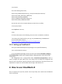
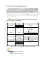
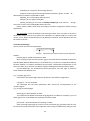
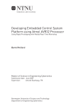
Download User`s Manual of CloudRank_V1.0

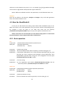
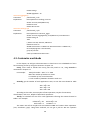
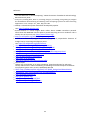
CloudRank-D
A Benchmark Suite for Private Cloud
USER’S MANUAL
June 15th
1
Contents
1. Background .................................................................................................................................... 4
2. Introduction of CloudRank-D .......................................................................................................... 4
2.1. CLOUDRANK -D ................................................................................................................................. 4
2.2. LICENSES OF CLOUDRANK-D ................................................................................................................. 4
2.3. WORKLOADS OF CLOUDRANK-D............................................................................................................ 5
2.3.1. Workloads in CloudRank-D ..................................................................................................... 5
2.3.2. Introduction of workloads ...................................................................................................... 5
2.4. ORIGINAL DATASET FOR WORKLOADS ...................................................................................................... 9
2.5. METHODOLOGY OF CLOUDRANK-D ...................................................................................................... 11
2.5.1. Skeleton ................................................................................................................................ 11
2.5.2. Configurable Workloads with Tunable Usage Patterns ........................................................ 12
2.5.3. Metric ................................................................................................................................... 14
3. Prerequisite Software Packages ................................................................................................... 15
3.1. BRIEF INTRODUCTION OF BASIC SOFTWARES ........................................................................................... 15
3.1.1. Hadoop ................................................................................................................................. 15
3.1.2. Mahout................................................................................................................................. 15
3.1.3. Hive ...................................................................................................................................... 16
3.2. SET UP............................................................................................................................................ 16
3.2.1. Setting up Hadoop................................................................................................................ 16
3.2.2. Setting up Mahout ............................................................................................................... 20
3.2.3. Setting up Hive ..................................................................................................................... 20
3.2.4. Setting up CloudRank-D ........................................................................................................ 21
4. How to use CloudRank-D .............................................................................................................. 21
4.1. FILES STRUCTURE AND EXPLANATION .................................................................................................... 22
4.2. RUN THE CLOUDRANK-D ................................................................................................................... 24
4.2.1. Basic operation ..................................................................................................................... 24
4.2.2. Classifier ............................................................................................................................... 25
4.2.3. Cluster .................................................................................................................................. 26
4.2.4. Recommendation ................................................................................................................. 27
4.2.5. Association rule mining ........................................................................................................ 27
4.2.6. Sequence learning ................................................................................................................ 28
4.2.7. Data warehouse operations ................................................................................................. 29
4.3. CUSTOMIZE WORKLOADS.................................................................................................................... 30
Reference......................................................................................................................................... 32
2
This document presents information on CloudRank-D --- a benchmark suite for private
cloud, including a brief introduction and the usage of it. The information and specifications
contained herein are for researchers who are interested in private cloud benchmarking.
Publishing information:
Release
Date
1.0
6/10/2013
Contact information:
Emails:
Website:
[email protected]
[email protected]
[email protected]
http://prof.ict.ac.cn/CloudRank/
3
1. Background
As information is growing explosively, more and more organizations are deploying private
cloud system to process massive data. Private cloud infrastructure is provisioned for exclusive
use by a single organization comprising multiple consumers (e.g., business units). It may be
owned, managed, and operated by the organization, a third party, or some combination of
them, and it may exist on or off premises1. However, there are few suitable benchmark
suites for evaluating private cloud. For these reasons, we propose a new benchmark suite,
CloudRank-D, to benchmark and rank private cloud computing system. We consider
representative applications, manifold data characteristics, and dynamic behaviors of both
applications and system software platforms into the design of CloudRank-D.
2. Introduction of CloudRank-D
In this part, we offer some basic information about CloudRank-D, particularly the workloads
in it. For users who care about the reason why we choose these applications as workloads,
please refer to the paper [2].
2.1. CloudRank -D
CloudRank-D focuses on evaluating private cloud system that is shared for running big
data applications. The first release consists of 13 applications that are selected based on their
popularity in today's private cloud system. These workloads are all from real application
scenarios which can help users get comparatively authentic system performance. The size of
datasets for workloads are scalable which can be adapted for different cluster size. Our
benchmark suite now runs on top of Hadoop3 framework, later will be extended to others.
So before using CloudRank-D, users need to install some basic softwares. More details about
installation in Chapter 3.
2.2. Licenses of CloudRank-D
CloudRank-D is available for researchers interested in pursuing research in the field of
private cloud and data centers. Software components of CloudRank-D are all available as
open-source softwares and governed by their own licensing terms. Researchers intending to
use CloudRank-D are required to fully understand and abide by the licensing terms of the
various components. For now, CloudRank-D is open-source under the Apache License,
Version 2.0. Please use all files in compliance with the License.
4
2.3. Workloads of CloudRank-D
2.3.1. Workloads in CloudRank-D
The workloads in CloudRank-D are some representative algorithms from seven
application scenarios which are frequently occurred in private cloud system showed in Table
1. We will elaborate these workloads in Section 2.3.2.
Num
Basic Operations
1
2
3
Applications
Sort
Word count
Grep
Source
Hadoop
Mahout and
Scientist search 4
(another one of
our work)
Classification
4
5
Naive bayes
Support vector machine
Clustering
6
K-means
Recommendation
7
Item based collaborative filtering
Association Rule Mining
8
Frequent pattern growth
Sequence Learning
9
Hidden markov model
Scientist search
Data Warehouse
Operations
10
11
12
13
Grep select
Rankings select
Uservisits aggregation
Uservisits-rankings join
Hive-bench
Mahout
Table 1 Workloads in CloudRank-D
2.3.2. Introduction of workloads
2.3.2.1.
Basic operation
Sort
The sort uses Hadoop Map/Reduce framework to sort the input data and write them
into the output directory. The inputs and outputs must be sequence files (a special data
format used in Hadoop) where the keys and values are BytesWritable (a kind of class in
Hadoop). Users can use some tools to change TXT files into sequence files which can break
this limitation. The Mapper and Reducer are predefined IdentityMapper and IdentityReducer
(default map/reduce function). Both of them just pass their inputs to the outputs with simple
process. There are some sorting process offered by Hadoop framework itself, which can sort
these data to get correct results.
WordCount
WordCount reads text files and counts the number of occurrence of each word. The
5
input is text files and the output is also text files that each line of the file contains a word and
its occurrence frequency, separated by a tab. Each Mapper takes a line as input and breaks it
into words, it then emits a key/value pair. Each Reducer sums the counts for each word and
emits a single key/value with the word and sum. As an optimization, the Reducer is also used
as a Combiner (similar to Reducer) on the map outputs, which reduces the amount of data
sent across the network by combining each word into a single record.
Grep
Grep extracts matching strings from text files and counts its frequency of occurrence.
The program runs two Map/Reduce jobs in sequence. The first job counts how many times a
matching string occurred and the second job sorts matching strings by their frequency and
stores the output in a single output file. Each Mapper of the first job takes a line as input and
matches the user-provided regular expression against the line. It extracts all matching strings
and emits (matching string, 1) pairs. Each Reducer sums the frequencies of each matching
string. The output is sequence files containing the matching string and frequency. The reduce
phase is optimized by running a Combiner that sums the frequency of strings from local map
output.
2.3.2.2.
Classifier
Naive Bayes
Naive Bayes classifier is a classical probabilistic classifier based on applying Bayes'
theorem with strong (naive) independence assumptions. Here we use the input data set to
drive the Mahout Naive Bayes classifier.
Input dataset is 20 Newsgroups showed later in Section 2.4. Mahout Bayes Classifier will
split dataset up into chunks. These chunks are then further split by country. From these splits,
a classifier is trained to predict what country an unseen article should be categorized into.
SVM--Support Vector Machines
In machine learning, support vector machines (SVMs, also support vector networks) are
supervised learning models with associated learning algorithms that analyze data and
recognize patterns, used for classification and regression analysis. The basic SVM takes a set
of input data and predicts, for each given input, which of two possible classes forms the
output, making it a non-probabilistic binary linear classifier. 5
2.3.2.3.
Cluster
K-means
K-means clustering is a method of cluster analysis which aims to partition n observations
into k clusters in which each observation belongs to the cluster with the nearest mean which
then put a partitioning of the data space into Voronoi 6 cells. The problem is computational
difficulty (NP-hard), however, there are efficient heuristic algorithms that are commonly
employed and converge fast to a local optimum. This process is iterative, additionally,
k-means clustering tends to find clusters of comparable spatial extent. 7
6
2.3.2.4.
Recommendation
Item-based Collaboration Filtering
Item-based collaboration filtering algorithm looks into the set of items. The target user
has been rated and computed how similar they are to the target item i and then selects k
most similar items {i1,i2,…,ik}. At the same time, their corresponding similarities {si1,si2,…,sik}
are also computed. Once the most similar items are found, the prediction is then computed
by taking a weighted average of the target user’s ratings on these similar items. We describe
these two aspects, namely, the similarity computation and the prediction generation in
details here.
Item A
User A
User B
Item B
User C
Item C
Figure 1
Similarity
An simple example for IBCF algorithm
Showed in Figure 1, if the user A likes items A and C, while the user B likes items A, B
and C, we can infer that items A and C is more similar items from the history of these users
preference. That is, if the user likes item A, he may also like item C and vice versa. Based on
the data, the user C is to like the item A, so the recommendation system will recommend
item C to the user C.
2.3.2.5.
Association rule mining
Frequent Pattern-Growth
The frequent pattern means patterns which appear frequently in the sample data sets,
such as item-sets, subsequences and substructures. Compared to the conventional frequent
pattern mining method Apriori, FP-growth extracts the concise information for frequent
pattern mining and stores it into a compact structure, which is called FP-tree. With the help
of FP-tree, FP-growth greatly reduces the price of Apriori.
The steps of FP-growth are as follows:
Firstly, database partition. Database is divided into consecutive partitions, and each
partition is located on different machines. Each of these partitions is called shard.
Secondly, computing the support count of each item. It can use a map/reduce job to
finish it. And the computing process is similar to the application of WordCount in Hadoop.
Thirdly, grouping. It divides entries in the F_list (F_list = {item1:count1, item2:count2,
item3:count3…} ^ (count1> count2 > count3>…)) into Q groups, which constitute a G_list.
Every group in the G_list is assigned a G_id, and each G_list contains a set of item collection.
7
Fourthly, parallel FP-growth. It uses the second map/reduce job to complete it. The
mapper completes the main function of database partition. It uses shard, mentioned in the
first step, to handle each transaction in the shard database partition. The transaction is
divided into items, and each item according to G_list is mapped to the right group. Through
the mapper, items belonging to the same group are converged to a machine. Based on the
complete data set from mapper, the reducer counts the result by FP-growth algorithm.
Last, aggregation. We get the final results from the aggregation of results on each
machine.
2.3.2.6.
Sequence learning
Hidden Markov Model
A HMM is a statistical Markov model in which the system being modeled is assumed to
be a Markov process with unobserved (hidden) states. In a Hidden Markov model, the state
is not directly visible, but the output, dependent on the state, is visible. Each state has a
probability distribution over the possible output tokens. Therefore the sequence of tokens
generated by an HMM gives some information about the sequence of states. Note that the
adjective 'hidden' refers to the state sequence through which the model passes, not to the
parameters of the model, even if the model parameters are known exactly, the model is still
'hidden'. A Hidden Markov Model can be considered a generalization of a mixture model
where the hidden variables (or latent variables), which control the mixture component to be
selected for each observation, are related through a Markov process rather than
independent of each other. 8
2.3.2.7.
Data Warehouse Operations
As we know, data are usually stored in data warehouse, so data warehouse operations
are significant workloads in cloud system, so we adopt some operations from Hive-bench.
Hive is a data warehouse tools based on Hadoop, and Hive-bench is a benchmark suite for it.
Grep Select
Grep Select is a Hive operation in the Hive-bench. There are two columns (key, field) in
Table Grep, and the main operation is to select the matching strings which is similar to the
Grep in basic operations. The difference is that operation here is done through the database.
Ranking Select
Table Ranking contains large amount of ranked URLs data, and have three columns
(pageRank, pageURL, avg Duration). Ranking Select is used to retrieve some URLs which fulfill
the requirements. This application aims to calculate the time of processing the large amount
data.
Uservisits Aggregation
In this operation, the data is the records of user visits. The output is the processing
result of the data. The operation processes the table data, calculates the total information
grouped by some requirements.
8
Uservisits-rankings Join
This operation is mainly about join operation. In Hive, only equality joins, outer joins,
and left semi joins are supported, because other join operations are not fit for map/reduce
framework. Hive converts joins over multiple tables into a single Map/Reduce job if for every
table the same column is used in the join clauses.
2.4. Original dataset for workloads
In this part, we will introduce the datasets which are used to drive algorithms. All of these
datasets have their own true semantics. Table 2 shows a description of dataset semantics.
Application
Data semantics
Sort
Wordcount
Automatically generated
Grep
Naive bayes
20news and wikipedia
Support vector machine
Scientist search
K-means
Sougou corpus
Item based collaborative filtering
Ratings on movies
Retail market basket data
Frequent pattern growth
Click-stream data of a on-line news portal
Traffic accident data
Collection of web html document
Hidden morkov model
Scientist search
Grep select
Ranking select
Automatically generated table
Uservisits aggregation
Uservisits-rankings join
Table 2
Semantics of Datasets.
Basic operation (Sort, WordCount, Grep)
The input data set for all these three workloads can be generated by using
RandomWriter and RandomTextWriter, which are provided by Hadoop itself. RandomWriter
writes 10 giga (by default) of random data to HDFS using Map/Reduce. Each map takes a
single file as input and writes random BytesWritable keys and values to the HDFS sequence
file. The maps do not emit any output and the reduce phase is not used. The specifics of the
generated data are configurable. 9 The configuration variables are:
Name
Default Value
test.randomwriter.maps_per_host
10
test.randomwrite.bytes_per_map
1073741824
9
Description
Number of maps/host
Number of bytes written/map
test.randomwrite.min_key
10
test.randomwrite.max_key
1000
minimum size of the
key in bytes
maximum size of the key in bytes
test.randomwrite.min_value
0
minimum size of the value
test.randomwrite.max_value
20000
maximum size of the value
Table 3
Common configuration variables in Hadoop
Classifier (Naive Bayes and SVM)
Naive Bayes:
Input data set: 20 Newsgroups
The 20 Newsgroups data set is a collection of approximately 20,000 newsgroup
documents, partitioned (nearly) evenly across 20 different newsgroups. The 20 newsgroups
collection has become a popular dataset for experiments in text applications of machine
learning techniques, such as text classification and text clustering. We will use Mahout Bayes
Classifier to create a model that would classify a new document into one of the 20
newsgroup. 10 This dataset is called wikipediainput in the package we provide.
SVM:
Dataset for SVM comes from Scientist Search. Scientist Search is a search engine, which
collects almost 227683 researchers’ personal information and 20005225 research webs to
provide searching service on academic.
Cluster (K-means)
We take sogou corpus as input of k-means algorithm. The data in sogou corpus comes
from a Chinese news website called Sohu, which collects almost 100 thousand documents
processed by hand finish. 11
Recommendation (Item based collaborative filtering)
These datasets are from MovieLens web site 12. MovieLens predicts rating that users give
to a movie based on existing data. When a new user logs in MovieLens, he needs to rate for
15 movies from 1 point to 5 point, with a 0.5 point interval, and these datasets will be used
as base data to predict user’s preference.
Association rule mining (Frequent pattern growth)
These data for association rule mining are real statistic information, including retail
market basket data, click-stream data of an on-line news portal, traffic accident data and
collection of web html document. 13
Sequence learning (Hidden morkov model)
The dataset for this application is also from Scientist Search, which is same as the
dataset for SVM mentioned above.
Data warehouse operation (Hive-bench)
There are three tables, including Table Grep, Table Ranking and Table Uservisits. Table
Grep contains two columns (key, field), Table Ranking is a sorted table of html pages with
three columns (pageRank, pageURL, kavgDuration), and Table Uservisits which records users
10
browsing history with nine columns (sourceIP, destURL, visitDate, adRevenue, userAgent,
countryCode, languageCode, searchWord, duration). These datasets are generated by data
generation tools, users can find them in our package under cloudrank-d/datagen/. The
introductions of these tools are given in 4.2.7.
2.5. Methodology of CloudRank-D
2.5.1. Skeleton
There is a system platform, users want to benchmark it, and they always running some
workloads on it, what’s more, they also hope these workloads can be come near the real
world workloads to make the results more receivable. Users also need some intuitional
directly observed metrics to estimate whether the system platform works well or not.
Through this statistics, they can feedback it to workloads, to get the peak system
performance then to achieve their goals. This procedure is showed below.
Figure 2
CloudRank-D Methodology
The real workloads account for much in system benchmarking, but for some reasons,
users can't get real workload as usual, then we need to simulate the workload more close to
real scenarios. Our benchmark is flexible to combine workloads to fit various scenarios, and
easy to extent, here, we also provide methods to let users adjust their workloads
approaching the ones in real world. Different from most existing benchmarks, workloads we
provide are independent separately, and for most of workloads, their input data size are
scalable, which allow users to customize their own workload combinations as wish. For
example, users can run application HMM with 2G or 4G, SVM with 4G and so on. Next, we
will introduce how to get more real workloads, relate contents also in our slide:
CloudRank-D: A Benchmark Suite for Private Cloud System.
Link: http://prof.ict.ac.cn/CloudRank/download.html
11
2.5.2. Configurable Workloads with Tunable Usage Patterns
2.5.2.1.
Scalable applications and input data sets
Obtain a suitable workloads combination
Firstly, users should estimate the total number of jobs they plan to run according to
basic information of cluster. We offer a simple formula here.
Formula 1:
Total job number = Number of machines in cluster * Number of cores in each machine *
Hardware threads number of each core
Users can use this formula to calculate a primitive total job number. Next, for simulating
more real workloads, we advise that users have a general idea about their jobs in advance.
Users may realize that there are more classification jobs in cluster, then they can raise the
proportion of classification workloads in total. If users don’t have such thoughts about their
own workloads, here, we give a reference ratio according the PowerBy page about Hadoop.
These statistic data comes from 2009.
Figure 3
The usage of percentages of applications in private clouds reported in
14
From this table, we can get a rough application ratio, now, we use this statistics to
construct the workloads ratio. We make workloads in CloudRank-D to accordance with the
statistic data by abstract main operations in them. For example, in Figure 3, reporting takes
17%, and in our benchmark, Hive-bench operations meet basic operations in reporting, so
we firstly set the ratio of Hive-bench jobs is 17%. Table below is listing the correspondence
between them. This is just a basic configuration, users can adjust it if need.
12
Text indexing
Log processing
Web crawling
Data mining
Machine learning
16%
15%
15%
7%
11%
Basic operations
Basic operations
Classification & Association Rule
Mining & Cluster & Recommendation
& Sequence learning
Reporting
Data storage
17%
17%
Hive-bench
Hive-bench
Table 4
Recommended ratio settings for workloads combination
For there are no image processing-like operations in our benchmark, users can add 2%
to other applications.
Now, if users want to run 200 jobs, then the number of each applications may like this.
Figure 4
An example of number of each applications
Configure the size of different applications
We introduce how to mix the workload from category dimension just now, here, we
change to take job size into account. So, how to set proportion of different size? We extent
statistic data from Taobao 15 report to job size. In Taobao report, the Map Number and its
percentage statistic is showed in Table 5. For each Map sets 128M, we can infer the jobs size
reversely, like results in Table 5.
Table 5 Job Size Statistics
13
2.5.2.2.
Jobs submission patterns
Submission interval
From the Facebook report 16, they sampled job inter-arrival times at random from the
Facebook trace, and this distribution of inter-arrival times was roughly exponential with a
mean of 14 seconds. Users can schedule their jobs according to this conclusion. Please notice
that, this is just Facebook's case, not fit for every environments, users can treat this as a
configuration parameters during the system testing.
Submission order
After getting the workloads, users also need to decide how to send them to the system.
There are some basic solutions, and users can send their workloads according to some other
methods. The most simply, users can sent workloads randomly, this submission order ignore
the relationship between jobs, like certain kind of workloads are sent intensively. Beside,
Users can submit several job from one kind of workloads firstly, then sent another. Because
different applications will use different components in cluster, like CPU bound applications
will occupy the CPU resource in cluster, and I/O bound applications will request for I/O
bandwidth, reasonable delivered sequence can make a important effect on cluster
performance.
2.5.3. Metric
We want to find a metrics which is directly perceived, and easy to compare and get. The
FLOPS (Floating-point operation per second) is used usually when to evaluate HPC (High
Performance Computing) cluster, but it's not fit for private cloud, because private cloud
focuses on the data processing, not the CPU capacity, what’s more, there are fewer
floating-point operations in private cloud than HPC cluster. So we need a metrics which can
reflect some other features, like disk I/O, or memory access. Now, we choose two intuitively
metrics:
Data processed per second / Data processed per joule
Users just need to record the total data input size, the total run time, and total energy
consumption (which need a power meter). The calculate formulas are:
DPS=Total data input size / Total run time
DPJ=Total data input size / Total energy consumption
14
3. Prerequisite Software Packages
Our benchmark suite is now deployed on Hadoop. We adopt some machine learning
algorithms from Mahout and some database operations based on Hive, so we also need to
install Mahout and Hive in advance.
Hadoop
We recommend version 1.0.2, which was used and tested in our environment.
Version 1.0.2 download link:
mirrors.tuna.tsinghua.edu.cn/apache/hadoop/common/hadoop-1.0.2
Other version:
http://www.fayea.com/apache-mirror/hadoop/common/
Mahout
We recommend mahout-distribution-0.6, which was used and tested in our
environment.
Download link:
http://mirrors.tuna.tsinghua.edu.cn/apache/mahout/
Hive
We recommend version 0.6.0, which was used and tested in our environment.
Download link:
http://hive.apache.org/releases.html#Download
CloudRank-D
CloudRank-D contain several algorithm implementation, scripts, and test data for users,
and users can download the whole package from our website.
Download link:
http://prof.ict.ac.cn/CloudRank/download.html
3.1. Brief introduction of basic softwares
3.1.1. Hadoop
Hadoop is a MapReduce implementation and contains two main components: the HDFS
file system and the MapReduce infrastructure. HDFS is short for Hadoop Distributed File
System, which supports to store data on low-cost hardware and is more suitable to deal with
applications with big data set. MapReduce is a kind of programming model and usually used
for distributed computing with data stored in the distributed file system. 17,18
3.1.2. Mahout
Mahout is an open-source program of Apache Software Foundation, which provides
several scalable machine learning and data mining algorithm implementation to help
developers conveniently develop intelligence applications. At present, there are three public
versions of mahout. Mahout includes cluster, classification, collaborative filtering and many
15
other classical algorithms. Moreover, it can be expanded into cloud application through the
library offered by Apache Hadoop. In our benchmark, we choose cluster, classification,
sequence learning, association rules mining and collaborative filtering recommendation from
Mahout.19
3.1.3. Hive
Hive is a data warehouse infrastructure in common use built on top of Hadoop for
providing data summarization, query, and analysis. Hive can change the structure data files
into a database table, provides integrated SQL functions, and also can put SQL carried out on
MapReduce.20
Please note: Hive is based on Hadoop, so users should ensure that there have installed
Hadoop before installing Hive.
3.2. Set up
3.2.1. Setting up Hadoop
As we mentioned above, our benchmark now runs on Hadoop framework, so we need
deploy Hadoop environment at first. To install Hadoop on cluster, users have to unpack the
Hadoop package on all the cluster nodes with same path. Here, we use $HADOOP_HOME to
stand for installation path, so the $HADOOP_HOME of each node should be the same.
What’s more, users should add $HADOOP_HOME into the system environment variable.
3.2.1.1.
Create a Hadoop user
Creating a Hadoop user can improve flexibility of system management. This requires
root privileges and the commands can be different in various Linux distributions such as
useradd vs adduser. Here, we give some common commands.
$ sudo groupadd hadoop
$ sudo useradd -g hadoop hadoop
$ sudo passwd hadoop (to setup the password)
3.2.1.2.
Preparing SSH
SSH (Secure Shell) is a common remote login session protocol. It can provide security
assurance for the machines message transfer. Here are the commands.
$ su - hadoop (switching user)
$ ssh-keygen -t rsa -p "" (generating assembly key file, press enter for any prompts)
$ cat ~/.ssh/id_rsa.pub >> ~/.ssh/authorized_keys
$ ssh localhost (answer yes to the prompt)
16
For more information, users can reference the following website:
http://www.openssh.org/
3.2.1.3.
Configuration on Hadoop
Hadoop is implemented in JAVA, so there should be JDK in machine. Put the Hadoop
package to the specified directory, then unpack the package. Here, we just give an example
for installation, users can specify own path as wish, and be sure that there are permissions
on relate files operations.
$ tar -zxvf hadoop-1.0.2.tar.gz
$ cd hadoop-1.0.2
Then set the user-group permissions,
$ chown -R hadoop:hadoop hadoop-package-name
Update the ~/.bashrc file (or an equivalent configuration file if use other shells) with the
following:
export HADOOP_HOME=/path/to/hadoop(e.g., /home/username/hadoop-1.0.2/)
export JAVA_HOME=/path/to/jdk(e.g., /usr/lib/jvm/java-6-sun)
In the HADOOP_HOME folder (the main Hadoop folder), make the following
modifications to the configuration files under directory conf. The main files users need to
modify are listed below:
hadoop-env.sh，core-site.xml ，hdfs-site.xml，mapred-site.xml，master and slaves
hadoop-env.sh
Editing the conf/hadoop-env.sh and specifying the Java JDK location (JAVA_HOME),
users need to set the JAVA_HOME according to their java installation path.
export JAVA_HOME=/path/to/jdk
core-site.xml
In conf/core-site.xml, add
<configuration>
<property>
<name>fs.default.name</name>
<value>hdfs://localhostname:9100</value>
</property>
</configuration>
17
hdfs://localhostname:port/ assign the host and the port.
hdfs-site.xml
In conf/hdfs-site.xml, add
<configuration>
<property>
<name>dfs.name.dir</name>
<value>/opt/hadoop/hadoopfs/name1,/opt/hadoop/hadoopfs/name2</value>
<description> description </description>
</property>
<property>
<name>dfs.data.dir</name>
<value>/opt/hadoop/hadoopfs/data1,/opt/hadoop/hadoopfs/data2</value>
<description> </description>
</property>
<property>
<name>dfs.replication</name>
<value>1</value>
</property>
</configuration>
dfs.name.dir is the file system path which enduringly stores the namespace and
transaction logs by NameNode.
dfs.data.dir is the local path for saving data by DataNode.
Parameter ‘replication’ represents the number of block replications. The default value is
3. It will warn if the number of machines in cluster is smaller than replication value.
Please notice：users had better not to create directory name1、name2、data1、data2 in
advance. Hadoop will create them after initialized. And, if users want to choose a folder of
themselves, please make sure the folder with read/write permissions.
mapred-site.xml
In mapred-site.xml, add
<configuration>
<property>
<name>mapred.job.tracker</name>
<value>node1:9200</value>
</property>
</configuration>
The host and port is at which MapReduce job tracker runs.
18
masters and slaves
Configuring the masters and slaves to set the NameNode and the DataNode, users had
better use the hostname, and ensure machines can communicate pairwise.
master：write the hostname of master into file
Example: node1
slaves：write the hostname of slaves into file
Example: node2
Please note: There are other parameters that should be tuned to fit different needs,
such as
mapred.tasktracker.map.tasks.maximum, mapred.tasktracker.reduce.tasks.maximum,
mapred.map.tasks, mapred.reduce.tasks.
For now we use the default values.
After configuring, users can copy the hadoop document to other nodes, and modify the
relate parameters in order to be suitable for new machines. For example, users have to
modify the JAVA_HOME according the new machines installation path.
Start and Stop
Users have to format a new distribute file system (HDFS) when the Hadoop is installed
first, here is the command.
$ cd hadooppackage
$ bin/hadoop namenode -format
Check the distribute file system, if success, there will be these two directories
/opt/hadoop/hadoopfs/name1 and /opt/hadoop/hadoopfs/name2 on master.
To start Hadoop, input the command below on master,
$ bin/start-all.sh
Master will start all slaves after executing this command. Users can check whether there
are /opt/hadoop/hadoopfs/data1 and /opt/hadoop/hadoopfs/data2 on master and slaves
to make sure it works. They can also use the command below to get the state of cluster.
$ bin/hadoop dfsadmin –report
To stop Hadoop, input the command below on master,
$ bin/stop-all.sh
Users need to input this command on master, then the master will close itself and the
19
slaves. All operations above will be recorded into log by daemon. Default path is
${HADOOP_HOME}/logs.
For more information about Hadoop installation, the following link provides a
step-by-step guide to install Hadoop on a single node.
Link: http://wiki.apache.org/hadoop/
3.2.2. Setting up Mahout
Unpack the package,
$ tar -zxvf mahout-0.6.tar.gz
It’s easy to install Mahout. Users just need to add Mahout path to env var of computer,
that is, modify the file .bashrc. The commands are，
$ vim /root/.bashrc
add,
export MAHOUT_HOME=/path/to/mahout-distribution-0.6
export PATH=${MAHOUT_HOME}/bin:${PATH}
make the change work,
$ source /root/.bashrc
test,
$ bin/mahout –help
If it lists much information about usage, that means it has installed the Mahout
successfully. Link:
https://cwiki.apache.org/MAHOUT/mahout-wiki.html#MahoutWiki-Installation%252FSetup
3.2.3. Setting up Hive
Entering the directory which put the Hive package, our suggestion is that users had
better put Hadoop package and Hive package on same directory to make management
convenient. Unzip the Hive compressed package,
$ tar -xzv hive-0.6.0-bin.tar.gz
modify the file .bashrc,
$ cd /root/
20
$ vim .bashrc
insert the following information,
export HIVE_HOME=path/to/hive(e.g.,/ home/username/hive-0.6.0-bin)
export HIVE_CONF_DIR=$HIVE_HOME/conf
export HIVE_LIB=$HIVE_HOME/lib
export CLASSPATH=$CLASSPATH:$HIVE_LIB
export PATH=$HIVE_HOME/bin/:$PATH
save the file, and run the command below to make the evn var effect,
$ soure /root/.bashrc
enter bin/hive to test Hive,
$ hive
If it shows information as the following, then users have succeeded to install hive.
“Hive history file=/tmp/root/hive_job_log_root_201208101534_1723482760.txt”
For more information, refer to:
https://cwiki.apache.org/Hive/adminmanual-installation.html
3.2.4. Setting up CloudRank-D
Users just need to decompress the package on the specified directory.
$ tar -zxvf cloudrank-d.1.0.tar.gz
In our CloudRank-D package, there are three main folders basedata, datagen，
and cloudrankrun, which store original dataset, data generation tools and scripts
respectively.
The configuration file is config.include under cloudrankrun/configuration/, which is
used to configure the path. Notice that, users always have to modify this configuration file
based on their environment. Specific parameters will be described on part files structure and
explanation in chapter 4.1 and the details about usage is described in 4.2.
4. How to use CloudRank-D
Now, we explain the scripts we provide. These scripts help users conduct the CloudRank-D
more conveniently.
21
4.1. Files structure and explanation
After unpacking the package, users will see three main folders basedata, cloudrankrun
and datagen. All the datasets we use are stored under basedata. While, under cloudrankrun,
there are several subfolders, including association rule mining, classification, hive-bench,
sequence-leaning, base-operations, cluster recommendation and configuration. Scripts for
each algorithm are placed in appropriate catalogs with almost same file structure, so here
we just give explanation on one or two of them. Under datagen, there are htmlgen and
teragen which are two tools to generate datasets used in data warehouse operations. We
will introduce them in 4.2.7.
basedata/
Table 6 lists the corresponding relationship between applications and original datasets.
The datasets can be seen under basedata/
Category
Application
Original Datasets
Sort
Base-operations
WordCount
Generated
Grep
Naive Bayes
Classification
wikipediainput (1.95G)
Support Vector
svm-data (1.96G)
Machine
Clustering
K-means
Recommendation
Association rule mining
Sequence-leaning
low(default)
sougou-low-tfidf-vec (121K)
mid
sougou-mid-tfidf-vec (4M)
high
sougou-high-tfidf-vec (16M)
Item based
ibcf-data (1.95G)
collaboration filtering
Frequent
pattern-growth
Hidden markov model
low(default)
fpg-accidents.dat (3.97M)
mid
fpg-retail.dat (33.86M)
high
fpg-webdocs.dat (1.38G)
hmm-data (1.95G)
Grep select
Hive-bench
Ranking select
Uservisits aggregation
Generated
Uservisits-ranking join
Table 6
The corresponding relationship between application and original datasets
cloudrankrun/
configuration/
Subfiles:
config.include: record related configurations
Parameters:
basedata_dir: data storage path in local
22
tempdata_dir: temporary data storage directory
Temporary data is generated during the data preparatory phase, and will be
deleted after final data are uploaded to HDFS.
hdfsdata_dir: corresponding HDFS directory
basejars_dir: the path of basic jars
hadoop_example_jar: the name of hadoop-examples-jar, users need to change
this name in terms of the Hadoop jars release they use.
Notice: please modify these paths according to machine configuration before running
applications.
file_all.include: record the datasets now existing on HDFS. Users can refer to this file to
write batch scripts. This file only reflects the operations on HDFS through our scripts, that
means, if user delete the datasets directly by Hadoop commands, these operations will not
be refresh in this file.
associationrulemining/
Here is the file structure and explanation:
associationrulemining/fpg/
Category
Abbreviation for Frequent pattern-growth Algorithm
Subfiles:
prepare-fpg.sh: upload the dataset to HDFS
After carrying out the command predict_fpg.sh, local data will be uploaded to HDFS with
specified path (Default HDFS directory is /cloudrank-out). This phase is prepared for Hadoop,
because Hadoop is a software framework that provides a distributed manipulation of vast
amount of data, so we need to use HDFS to support Hadoop distributed processing ability.
For this application, the command has three parameters: low, mid, high, to stand for
three datasets with different size.
e.g.: ./prepare-fpg.sh low
It will choose the dataset fpg-accidents.dat which is also default configuration.
run-fpg.sh：run the workload
This command also has three parameters with one-to-one correspondence to the
“prepare-fpg.sh” .
e.g: run-fpg.sh low/mid/high
delete-fpg.sh: delete dataset on HDFS
This command will delete the dataset of fpg algorithm on HDFS. For example, if you run
delete-fpg.sh low, it will delete low size dataset stored on HDFS.
file.include : stores the dataset now existing on HDFS
After executing prepare-fpg.sh, there are some records like fpg_file=XXX in this file. This
file stores the name of datasets of this algorithm now existing on HDFS which will give users
23
reference to select dataset they want to run. For example, fpg_file=fpg-webdocs.dat-high,
means there are fpg-webdocs with parameter high on HDFS now.
Notice: Different workloads have their own parameters, we will elaborate them in 4.2.
datagen/
There are two folders in this directory, htmlgen and teragen. They are all data generation
tools, more details showed in 4.2.7.
4.2. Run the CloudRank-D
In this part, we will describe the testing scripts which make CloudRank-D easy to use.
When users want to run some applications, they just need to execute corresponding scripts.
For example, if users are going to run SVM, they enter into the directory
/cloudrankrun/classification/SVM/ to get its scripts, then type the command to run it.
Please notice that users should make sure the dataset storage path is in accord with
the specified path in script config.include under /cloudrankrun/.
4.2.1. Basic operation
Sort
Scripts path:
HDFS path:
Command:
/cloudrank-d/cloudrankrun/base-operations/sort
/cloudrank-data/ (input)
/cloudrank-out/
(output)
./prepare-sort.sh 10g
Parameter： the size of dataset users want to specify, it can be m/M, g/G, t/T.
Explanation: it will produce 10GB data for sort. Script will adjust parameter byte_per_map
and maps_per_host in config-sort.xml according to current deployment. Then
RandonWriter generates data using this new configuration file with path
/cloudrank-data/rtw-sort-10G on HDFS.
Command:
./run-sort.sh 10g
Explanation: run sort application with dataset /cloudrank-data/rtw-sort-10G, and the
results are placed in /cloudrank-out/rtw-sort-10G-out on HDFS.
Wordcount
Scritps path: /cloudrank-d/cloudrankrun/base-operations/wordcount
HDFS path: /cloudrank-data/
(input)
/cloudrank-out/
(output)
Command:
Parameter:
./prepare-wordcount.sh 10g
the size of dataset users want to generate, it can be m/M, g/G, t /T.
24
Explanation:
it will produce 10g dataset for wordcount. Script will adjust parameter
byte_per_map and maps_per_host in config-sort.xml according to current
deployment. Then RandontextWriter generates dataset using this new
configuration file with path /cloudrank-data/rtw-wordcount-10G on HDFS.
Command： ./run-wordcount.sh 10g
Explanation: run with dataset /cloudrank-data/rtw-wordcount-10G, and the results are
/cloudrank-out/rtw-workcount-10G-out on HDFS.
Grep
Scritps path:
HDFS path:
Command:
Parameter:
Explanation:
/cloudrank-d/cloudrankrun/base-operations/grep
/cloudrank-data/ (input)
/cloudrank-out/ (output)
./prepare-grep.sh 10g
the size of dataset users want to generate, it can be m/M, g/G, t/T.
it will produce 10g dataset for grep. Script will adjust parameter
byte_per_map and maps_per_host in config-sort.xml according to current
deployment. Then RandontextWriter generates dataset using this new
configuration file with path /cloudrank-data/rtw-grep-10G on HDFS.
Command： ./run-grep.sh 10g
Explanation: run grep with dataset /cloudrank-data/rtw-grep-10G, and the results are
placed in /cloudrank-out/rtw-grep-10G-out on HDFS.
4.2.2. Classifier
Naive Bayes
Scripts path: /cloudrank-d/cloudrankrun/classification/NaiveBayes/
Dataset path: /basedata/wikipediainput
HDFS path:
/cloudrank-data/ (input)
/cloudrank-out/
(output)
Command:
./prepare-bayes.sh 2
Parameter： the multiple of original dataset users want to expand.
Explanation: execute the data preparation, it will copy the original dataset according to
parameter, then upload the new dataset onto the HDFS. The new dataset path
is /cloudrank-data/bayes-SIZE. For example, if the basic dataset is 2.1G, then
the new dataset will be /cloudrank-data/bayes-4.2G on HDFS.
Command： ./run-bayes.sh 2
parameter：
the parameter here is corresponding to that in prepare-bayes.sh.
Explanation： This command will choose dataset bayes-4.2G to run bayes application. The
dataset must be generated in advance. Users can refer to file.include to check
the dataset now existing on HDFS. The result will be at
25
/cloudrank-out/bayes-4.2-out.
Command:
Parameter:
Explanation:
./delete-bayes.sh 2
to delete extended data with 2 multiple of basic dataset on HDFS
delete dataset on HDFS, for this command, it will delete the dataset
bayes-4.2G on HDFS.
Support Vector Machine
Scripts path： /cloudrank-d/cloudrankrun/classification/SVM/
Dataset path： /basedata/svm-data
HDFS path:
/cloudrank-data (input)
/cloudrank-out (output)
Command:
./prepare-svm.sh 2
Parameter： the multiple of original dataset
Explanation: execute the data preparation. It will copy the original dataset according to
parameter, then upload the new dataset onto the HDFS. The new dataset path
is /cloudrank-data/svm-SIZE. For example, if the basic dataset is 2.1G, then
the new dataset is stored at /cloudrank-data/svm-4.2G on HDFS.
Command： ./run-svm.sh 2
Parameter:
in accordance with prepare-ibcf.sh, used to specify dataset
Explanation: execute the SVM program with the specified dataset. For this command, it will
run application with dataset SVM-4.2G (same as above). The dataset must
be generated in advance. Users can refer to file.include to check the dataset
now existing on HDFS. The result will be at /cloudrank-out/svm-4.2-out.
Command:
Parameter:
Explanation:
./delete-svm.sh 2
to delete extended data with 2 multiple of basic dataset on HDFS
delete dataset on HDFS, for this command, it will delete the dataset
SVM-4.2G (same as above) on HDFS.
4.2.3. Cluster
K-means
Scripts path:
Input：
HDFS path:
Command:
Parameter:
Explanation:
/cloudrank-d/cloudrankrun/cluster/kmeans/
/basedata/sougou-low-tfidf-vec
/basedata/sougou-mid-tfidf-vec
/basedata/sougou-high-tfidf-vec
/cloudrank-data
(input)
/cloudrank-out
(output)
./prepare-kmeans.sh low|mid|high
low|mid|high (represent the dataset with different size)
upload the basic dataset to the HDFS, and the path is /cloudrank-data/.
26
Command： ./run-kmeans.sh low|mid|high
Parameter： low|mid|high (represent the dataset with different size)
Explanation： the relationship between the parameter and the dataset is showed
below.
Parameter
Input(HDFS)
Output (HDFS)
low
/cloudrank-data/sougou-low-tfidf-vec
/cloudrand-out/kmeans-low-out
mid
/cloudrank-data/sougou-mid-tfidf-vec
/cloudrand-out/kmeans-mid-out
high
/cloudrank-data/sougou-high-tfidf-vec
/cloudrand-out/kmeans-high-out
Command:
./delete-kmeans.sh low|mid|high
Parameter：
low|mid|high (represent the dataset with different size)
Explanation:
delete the corresponding dataset on HDFS.
4.2.4. Recommendation
Item based collaboration filtering
Scripts path: /cloudrankrun/recommendation/ibcf/
Input:
/basedata/ibcf-data
HDFS path: /cloudrank-data (input)
/cloudrank-out (output)
Command： ./prepare-ibcf.sh 2
Parameter： 2 is the multiple of original dataset users want to expand
Explanation： execute the data preparation. It will copy the original dataset, then upload the
new dataset to HDFS. The new dataset path is /cloudrank-data/ibcf-SIZE. For
example, if the basic dataset is 12MB, then the new dataset is stored at
/cloudrank-data/ibcf-24M on HDFS.
Command： ./run-ibcf.sh 2
Parameter:
in accordance with prepare-ibcf.sh, used to specify dataset
Explanation: execute the IBCF program with the specified dataset. For this command, it will
run application with dataset ibcf-24M (same as above). The dataset must be
generated in advance. Users can refer to file.include to check the dataset now
existing on HDFS. The result will be stored at /cloudrank-out/ibcf-24M-out.
Command:
./delete-ibcf.sh 2
Parameter:
to delete extended data with 2 multiple of basic dataset on HDFS
Explanation: delete dataset on HDFS, for this command, it will delete the dataset ibcf-24M
on HDFS.
4.2.5. Association rule mining
Frequent pattern-growth
27
Script path: /cloudrank-d/cloudrankrun/associationrulemining/fpg/
Input data set: /basedata/fpg-accidents.dat
/basedata/fpg-retail.dat
/basedata/fpg-webdocs.dat
HDFS path： /cloudrank-data (input)
/cloudrank-out (output)
Command： ./prepare-fpg.sh low|mid|high
Parameter： low|mid|high respects the different data sets
Explanation: this command will send the specified dataset to HDFS.
Command： ./run-fpg.sh low|mid|high
Parameter： low|mid|high respects the different data set
Explanation： the relationship between the parameter and the dataset is showed
below.
Parameter
low
Input（HDFS）
/cloudrank-data/fpg-accidents.dat
Output（HDFS）
/cloudrand-out/fpg-low-out
mid
/cloudrank-data/fpg-reduce.dat
/cloudrand-out/fpg-mid-out
high
/cloudrank-data/fpg-webdocs.dat
/cloudrand-out/fpg-high-out
4.2.6. Sequence learning
Hidden markov model
Scripts path: /cloudrank-d/cloudrankrun/sequence-leaning/
Input data set: /basedata/hmm-data
HDFS path:
/cloudrank-data
(input)
/cloudrank-out
(output)
Command:
./prepare-hmm.sh 2
Parameter: 2 is the multiple of basic dataset users want to expand
Explanation: expand the basic dataset according to parameter, then upload new dataset to
HDFS. HDFS path is /cloudrank-data/hmm-SIZE. For example, if basic dataset
is 510M, then the new dataset is /cloudrank-data/hmm-1020M.
Command： ./run-hmm.sh 2
Parameter:
to drive hmm application with 2 multiple extended data
Explanation: execute the HMM program with the specified dataset. For this command, it
will run application with dataset hmm-1020M. The dataset must be generated
in advance. Users can refer to file.include to check the dataset now existing on
HDFS. The result will be stored at the /cloudrank-out/hmm-SIZE-out on HDFS.
Command:
./delete-hmm.sh 2
28
Parameter:
Explanation:
to delete extended data with 2 multiple of basic dataset on HDFS
delete dataset on HDFS, for this command, it will delete the dataset
hmm-1020M on HDFS.
4.2.7. Data warehouse operations
To run this application, firstly, users need to use data generation tools to generate
dataset. These tools can specify size of dataset, the things users need to do is just modifying
the configuration.
Folders htmlgen and teragen under /datagen store all scripts, and htmlgen will
produce two tables called Ranking01.data and UserVisits01.data with specified size, while,
teragen will produce Table Grep.
htmlgen:
Scripts path:
/cloudrank-d/datagen/htmlgen/
Command:
./generateData.py
Explanation:
The configuration file is config.txt, users can change the Rowcount for
UserVisits to decide the size of dataset. And, users need to specify the path
that stores the generated dataset, because this tool will delete the files
under the specified directory, our suggestion is to create a new directory to
store the dataset, then move them to /cloudrank-d/basedata/.
teragen:
Scripts path:
/cloudrank-d/datagen/teragen
Command:
sh teragen.pl
Explanation: The configuration file is teragen.pl itself. Users can modify the parameter
NUM_OF_RECORDS to specify the size of data.
Scripts path:
HDFS path:
/cloudrank-d/cloudrankrun/hive-bench/
/data/grep/
(input)
/data/ranking/
(input)
/data/uservisits/
(input)
/output/hadoop_bench/
(output)
Notice: Users need to create these folders on HDFS in advance.
Command:
Explanation:
Grep select
Command:
Explanation：
Ranking select
Command：
Explanation：
./prepare.sh
upload datasets to HDFS with path showed above.
./benchmark_gs.sh
main operation in grep_select
SELECT *
FROM grep
WHERE field LIKE '%XYZ%'
./benchmark_rs.sh
main operation in rankings_select
SELECT pageRank, pageURL
29
FROM rankings
WHERE pageRank > 10
Uservisits aggregation
Command：
Explanation：
./benchmark_ua.sh
main operation in rankings, uservist
SELECT sourceIP, SUM(adRevenue)
FROM uservisits
GROUP BY sourceIP
Uservisits-rankings Join
Command：
./benchmark_ruj.sh
Explanation：
main operation in uservisits_aggre
SELECT sourceIP, avg(pageRank), sum(adRevenue) as totalRevenue
FROM rankings R
JOIN
( SELECT sourceIP, destURL, adRevenue
FROM uservisits UV
WHERE UV.visitDate > '1999-01-01' AND UV.visitDate < '2000-01-01' )
NUV ON (R.pageURL = NUV.destURL)
group by sourceIP
order by totalRevenue DESC limit 1
4.3. Customize workloads
In this chapter, we will give a demonstration to show how to use CloudRank-D if users
have a existing cluster by using the contents in chapter 2.5.
Firstly, users need to decide how many jobs they need to run, using Formula 1
mentioned in chapter 2.5.
For example:
Total job number = 100 * 2 * 1 =200
100 is the number of machine in cluster
2 is number of core in each machine
1 is the number of hardware threads in each core
Secondly, get the number of each applications. Here, we use the ratio showed in Table
4.
200 * 31% = 62
200 * 35% = 70
200 * 34% = 68
According to this value, we set 62 jobs of basic operations, 70 jobs of association,
classifications, and so on, 68 jobs of Hive-bench operations.
Thirdly, we calculate the size of for each applications referring the statistic showed in
Table 5. For example:
62*40.57%＝26
62*39.33%＝24
62*12.03%＝7
62*8.07%＝5
This means we will set 26 jobs with size between 128M and 1.25G in basic operations
(sort, wordcount, grep). Using these methods, we can get a job list. We use exponent
30
distribution with 14s to generate random variable which means the interval between two
jobs, and can send job using random model.
Lastly, users can use script we provide to process these workloads in batch. Later, we
will offer a automation tool to put all these producers in integration.
An example of scripts usage.
Preparation phase
prepare.sh
cd associationrulemining/fpg/
sh prepare-fpg.sh high
cd ../..
cd classification/NaiveBayes
sh prepare-bayes.sh 1
cd ../..
cd classification/svm
sh prepare-svm.sh 1
sh prepare-svm.sh 2
cd ../..
This script uploads association rule mining with high parameter, bayes with original size
(2G), and svm with original size(2G) to HDFS.
Running phase
run.sh
cd associationrulemining/fpg/
sh run-fpg.sh high
cd ../..
sleep 2s
cd classification/NaiveBayes
sh run-bayes.sh 1
cd ../..
sleep 2s
cd classification/svm
sh run-svm.sh 1
sh run-svm sh.2
cd ../..
This script runs these three workloads, please notice that users should also input the
command with parameter, because maybe there are more than one dataset for one
application. More, users can use perf 21 or vTune 22 to capture the machine performance
statistical data to further their researches.
31
Reference
1
2
3
4
5
6
7
8
9
10
11
12
13
14
15
16
17
18
19
20
21
22
"The NIST Definition of Cloud Computing". National Institute of Standards and Technology.
Retrieved 24 July 2011.
Chunjie Luo, Jianfeng Zhan, Zhen Jia, Lei Wang, Gang Lu, Lixin Zhang, Cheng-Zhong Xu, Ninghui
Sun.CloudRank-D: Benchmarking and Ranking Cloud Computing Systems for Data Processing
Applications. Front. Comput. Sci., 2012, 6(4): 347–362
Hadoop is a distributed system framework developed by Apache.
Link: http://hadoop.apache.org/
Scientist Search is a search engine which collect almost 227683 researchers personal
information and 20005225 research webs to provide searching service on academic. This is
another one of our work. Link: http://www.zhisou.org/
http://en.wikipedia.org/wiki/Support_vector_machine
Voronoi is a continuous polygon composed by a group of perpendicular bisectors of
straight line by connecting two adjacent points.
Link: http://en.wikipedia.org/wiki/Voronoi
http://en.wikipedia.org/wiki/K-means_clustering
http://en.wikipedia.org/wiki/Hidden_Markov_model
http://wiki.apache.org/hadoop/RandomWriter
http://kdd.ics.uci.edu/databases/20newsgroups/20newsgroups.html
http://www.sogou.com/labs/dl/c.html
http://www.grouplens.org/node/73
http://fimi.ua.ac.be/data/
http://wiki.apache.org/hadoop/PoweredBy
Taobao report
Zaharia, M., D. Borthakur, et al. Delay scheduling: A Simple Technique for Achieving
Locality and Fairness in Cluster Scheduling. Proceedings of the 5th European Conference
on Computer System. Paris, France, ACM(2010),265-278
HDFS: http://hadoop.apache.org/docs/r1.0.4/hdfs_design.html#Introduction
MapReduce: http://en.wikipedia.org/wiki/MapReduce
http://mahout.apache.org/
http://hive.apache.org/
http://en.wikipedia.org/wiki/Perf
http://en.wikipedia.org/wiki/Vtune
32