1
The Bio-PEPA Workbench:
User’s Manual
Stephen Gilmore
The University of Edinburgh
April 24, 2009
Contents
1 Introduction
2
2 Example 1: Simple Michaelis-Menten kinetics
2.1 A Bio-PEPA model . . . . . . . . . . . . . . . . . . . . . . . .
2.2 Parameter information . . . . . . . . . . . . . . . . . . . . . .
3
3
5
3 Example 2: Michaelis-Menten with synthesis
3.1 The Bio-PEPA model . . . . . . . . . . . . . . . . . . . . . .
3.2 Plotting with model components . . . . . . . . . . . . . . . .
5
5
6
4 Installing the Bio-PEPA Workbench
4.1 Downloading and installing The Bio-PEPA Workbench . . . .
4.2 Download . . . . . . . . . . . . . . . . . . . . . . . . . . . . .
4.2.1 The Bio-PEPA Workbench . . . . . . . . . . . . . . .
6
6
7
7
5 Running the Bio-PEPA Workbench
8
6 Configuring the Bio-PEPA Workbench
6.1 Configuring simulations . . . . . . . . .
6.2 Configuring the number of replications .
6.3 StochKit options . . . . . . . . . . . . .
6.4 Reporting options . . . . . . . . . . . .
7 Extending the Bio-PEPA Workbench
.
.
.
.
.
.
.
.
.
.
.
.
.
.
.
.
.
.
.
.
.
.
.
.
.
.
.
.
.
.
.
.
.
.
.
.
.
.
.
.
.
.
.
.
.
.
.
.
8
8
10
10
11
11
8 Report generation
12
8.1 Web page . . . . . . . . . . . . . . . . . . . . . . . . . . . . . 12
8.2 LATEX report . . . . . . . . . . . . . . . . . . . . . . . . . . . 12
1
9 Troubleshooting
9.1 “Command not found” errors . . .
9.2 “Permission denied” errors . . . . .
9.3 “Cannot execute binary file” errors
9.4 “Cannot open” errors . . . . . . .
9.5 “Invalid parameter” errors . . . . .
9.6 “Undefined variable” errors . . . .
1
.
.
.
.
.
.
.
.
.
.
.
.
.
.
.
.
.
.
.
.
.
.
.
.
.
.
.
.
.
.
.
.
.
.
.
.
.
.
.
.
.
.
.
.
.
.
.
.
.
.
.
.
.
.
.
.
.
.
.
.
.
.
.
.
.
.
.
.
.
.
.
.
.
.
.
.
.
.
.
.
.
.
.
.
.
.
.
.
.
.
13
13
13
13
13
13
14
Introduction
This document describes the Bio-PEPA Workbench version 1.0 “Charlie
Mingus”, a tool for assisting with the analysis of systems which are modelled
in the Bio-PEPA process algebra. The definitive reference for Bio-PEPA is
the technical report “Bio-PEPA: a framework for the modelling and analysis
of biological systems” by Federica Ciocchetta and Jane Hillston1 .
The Bio-PEPA Workbench and accompanying documentation such as
this document can be obtained via the World-Wide Web from the address
http://homepages.inf.ed.ac.uk/stg/software/biopepa/.
Given a Bio-PEPA model the Workbench generates a simulation model,
a Markov chain model and a differential equation model. Thus the tool
enables the modeller to switch between discrete-state analysis via simulation
and model-checking and continuous-space analysis via differential equations
while maintaining only a single source model in the Bio-PEPA language.
The Bio-PEPA Workbench is intended for use with the stochastic simulation toolkit “StochKit”, which features an implementation of the wellknown stochastic simulation algorithm (SSA) of Gillespie. When given a
Bio-PEPA model the Bio-PEPA Workbench automatically generates other
representations in forms suitable for simulation and model-checking. The
generated simulation model contains the stoichiometry matrix and propensity functions in the form of C++ code which is linked against the StochKit
simulation library for simulation with Gillespie’s Direct Method.
The Bio-PEPA Workbench generates the differential equation model in
terms of a high-level “vector field” representation used by the VFgen software tool to generate ODE models suitable for analysis with the Sundials
ODE suite, Matlab, or many other tools.
The representation which is used for discrete state-space generation and
analysis by numerical solution of the underlying CTMC is expressed in the
reactive modules language supported by the PRISM model-checker. PRISM
provides algorithms for steady-state and transient analysis of continuoustime Markov chains and model-checking of logical formulae against CTMCs.
In addition the Bio-PEPA Workbench generates reward structures and common CSL formulae used in model-checking.
1
Available from http://www.inf.ed.ac.uk/publications/report/1231.html
2
2
Example 1: Simple Michaelis-Menten kinetics
We describe the components of the Bio-PEPA input language for the Workbench via a simple example. Consider Michaelis-Menten kinetics:
k1
k2
E + S E:S → E + P
k−1
where an enzyme E combines with a substrate S to form a compound E:S.
This compound might degrade releasing the enzyme and the substrate or it
might convert the substrate into product P , releasing the enzyme.
2.1
A Bio-PEPA model
We could encode this model in Bio-PEPA as shown below.
r1 = [k1 × E × S]
r−1 = [k−1 × E:S ]
r2 = [k2 × E:S ]
E = r1 ↓ + r−1 ↑ + r2 ↑
S = r1 ↓ + r−1 ↑
E:S
(E
= r1 ↑ + r−1 ↓ + r2 ↓
P
= r2 ↑
(S
{r1 ,r−1 ,r2 }
(E:S P )))
{r }
{r1 ,r−1 }
2
We have made use of aspects of the mathematical syntax for Bio-PEPA in
this definition. Before simulating this model we first need to encode it in
the syntax accepted by the Workbench. We place these definitions in the
file mm.biopepa. This is a plain text file which can be edited using a text
editor such as TextPad or Emacs. That file is shown in Figure 1.
In order to help with understanding the Bio-PEPA model the Bio-PEPA
Workbench generates a visualisation of the model in the form of a reaction
network graph where the species are represented as circles and the reactions
are represented using boxes. This is a directed graph where an arc leads
from a species to a reaction if that species is a reactant consumed by the
reaction. An arc leads in the other direction (from a reaction to a species)
if that species is a product formed by the reaction. An example of such a
network is shown in Figure 2.
3
% Bio-PEPA model of Michaelis-Menten kinetics
r1 = [k1 * E * S];
rm1 = [km1 * E:S];
r2 = [k2 * E:S];
E =
S =
E:S
P =
r1<< + rm1>> + r2>> ;
r1<< + rm1>> ;
= r1>> + rm1<< + r2<< ;
r2>> ;
(E <r1, rm1, r2> (S <r1, rm1> (E:S <r2> P)))
Figure 1: The mm.biopepa file
E
r1
E:S
rm1
S
r2
P
Figure 2: The reaction network graph generated from the mm.biopepa file
4
2.2
Parameter information
Before we can simulate the model we require parameter data in the form of
the initial molecular counts of the four species involved (E, S, E:S and P )
and the three rate constants (k1 , k−1 and k2 ). These should be stored in a
comma-separated value file named mm.csv. That file is shown in Figure 3.
E,
100,
100,
100,
S,
100,
100,
100,
E:S,
0,
0,
0,
P,
0,
0,
0,
k1,
1,
0.1,
0.01,
km1,
0.1,
0.1,
0.1,
k2
0.01
0.01
0.01
Figure 3: The mm.csv file
Space characters in the file are not significant and are only included for
readability above. Comma-separated value files are also text files and can
be edited using text editors such as TextPad or Emacs but they can also be
conveniently edited using spreadsheet applications such as Microsoft Excel
or OpenOffice oocalc.
3
Example 2: Michaelis-Menten with synthesis
We will now consider a slightly more complex example which illustrates
other features of the Bio-PEPA language. We will consider an example of
Michaelis-Menten with synthesis.
3.1
The Bio-PEPA model
There are four reaction channels in the model. Reaction r0 represents synthesis (of compound E:S ) at the constant rate k0 . The other three reactions
are the usual Michaelis-Menten enzymatic reactions.
r0 = [k0 ]
r1 = [k1 × E × S]
r−1 = [k−1 × E:S ]
r2 = [k2 × E:S ]
Five species are involved in the reactions. These are the enzyme E, the
substrate S, the compound E:S, the product P and the catalyst X, which is
needed to synthesize the compound E:S.
E = r1 ↓ + r−1 ↑ + r2 ↑
S = r1 ↓ + r−1 ↑
5
E:S
P
= r0 ↑ + r1 ↑ + r−1 ↓ + r2 ↓
= r2 ↑
X = (r0 , 1) X
The component T does not represent a chemical species. It is a model
component used to plot functions of the species numbers. In this case T is
merely the sum of the number of molecules of the species involved in the
reactions. The compound E:S is counted as two molecules.
T
= [E + S + (2 × E:S ) + P + X]
The species are involved in the reactions as described in the model equation
below.
(E
3.2
{r1 ,r−1 ,r2 }
(S
((X E:S ) P )))
{r }
{r }
{r1 ,r−1 }
0
2
Plotting with model components
Occasionally it is convenient to have a series plotted which is a function of
some other series computed during the simulation. It would be possible to
instrument a Bio-PEPA model with other species whose purpose was just to
generate these series but this would clutter the model. Model components
allow us to do this without cluttering the model. Consider X below.
X = [ A + B ];
X is a model component whose function is to compute the numerical sum of
the value of A and B (where A and B are species defined in Bio-PEPA in the
usual way). Model component X should not participate in any reactions and
any initial value supplied for X in the parameter file will be ignored (because
its value is computed as the sum of A and B). Such a model component is
used in our example of Michaelis-Menten with synthesis to track the total
number of molecules in the system. This is not a constant for this example
because molecules can be synthesised from an outside source.
4
Installing the Bio-PEPA Workbench
4.1
Downloading and installing The Bio-PEPA Workbench
A Linux-like environment with Bash is required to run the Bio-PEPA Workbench. We have tested the Workbench on 32-bit architectures Fedora Core
6 Linux and with Cygwin on Windows XP. We have tested the Workbench
on 64-bit SUSE Linux. The Bio-PEPA Workbench is implemented in Standard ML and currently uses the Moscow ML2 implementation as its runtime.
2
http://www.dina.kvl.dk/~sestoft/mosml.html
6
To run the Bio-PEPA Workbench you will need to have Moscow ML installed
on your machine. Under Cygwin we recommend that you install Moscow
ML in C:\mosml. The Bio-PEPA Workbench uses the StochKit3 stochastic
simulation toolkit to perform exact stochastic simulations using Gillespie’s
SSA algorithm. The StochKit framework uses the SPRNG random number generators4 if they are available, but can function without these. The
SPRNG random number generators require you to have a Fortran compiler
installed. We have used StochKit with SPRNG Version 2.0 but we have also
used StochKit without SPRNG.
The Bio-PEPA Workbench uses t5 o provide an intermediate representation of differential equations in XML format. The VFgen tool translates
these into programs which are executable as C code linked against the SUNDIALS6 ODE library or Matlab7 .
The Bio-PEPA Workbench uses Dot8 to draw reaction networks, Gnuplot9 to plot graphs and ImageMagick10 to display these. The LaTeX11
document preparation system is used to produce reports. You need to have
Dot, Gnuplot, ImageMagick and LaTeX available on your machine to run
the Bio-PEPA Workbench.
4.2
Download
4.2.1
The Bio-PEPA Workbench
Download StochKit for Linux12 or StochKit for Windows/Cygwin13 and the
current release of the Bio-PEPA Workbench14 . Unpack the file which you
got using one or other of the following two commands.
tar zxvf stochkit.tar.gz
unzip stochkit.zip
Unpack the Bio-PEPA workbench into the same directory.
unzip bpwb.zip
3
http://www.engineering.ucsb.edu/~cse/StochKit/index.html
http://sprng.cs.fsu.edu/
5
http://www.warrenweckesser.net/vfgen/>VFgen
6
https://computation.llnl.gov/casc/sundials/main.html
7
http://www.mathworks.com
8
http://www.graphviz.org/
9
http://www.gnuplot.info
10
http://www.imagemagick.org/
11
http://www.latex-project.org/
12
stochkit.tar.gz
13
stochkit.zip
14
bpwb.zip
4
7
Your directory should look like this.
bpwb stochkit
Change to the Bio-PEPA Workbench directory and make the Bio-PEPA
command executable.
cd bpwb
chmod +x bp
Run the Bio-PEPA Workbench. The following command runs the Bio-PEPA
Workbench over all .biopepa files in the current working directory.
./bp
If the above command did not work then it may be necessary to re-compile
the Bio-PEPA Workbench for your platform and then re-run the command.
(cd src ; make)
./bp
5
Running the Bio-PEPA Workbench
The Bio-PEPA Workbench can be run by issuing the command ./bp to
compile the input Bio-PEPA model, include the parameters from the model
parameter file and generate a report. The output from the command should
be similar to the output shown in Figure 4.
6
Configuring the Bio-PEPA Workbench
The behaviour of the Bio-PEPA Workbench can be configured by editing a
configuration file, biopepa.cfg. The current version of this file is shown in
Figure 5.
6.1
Configuring simulations
The simulator which is used to perform the simulation runs over the generated simulation model is specified by the parameter biopepa.simulator.
The stop time of the simulation run is specified in the numerical parameter value biopepa.simulation.stoptime. Any particular simulation run
might terminate before this stop time is reached if the reaction has run to
completion already. The defaults in the biopepa.cfg file are shown below.
biopepa.simulator: stochkit
biopepa.simulation.stoptime: 1000
8
Bio-PEPA Workbench Version 0.9.9 "Chad Smith" [25-August-2008]
Processing input from mm.biopepa
Compiling the model
Reaction channels: r1, rm1, r2
Species defined: E, S, E:S, P
Model components defined:
Starting Dot file compilation.
Finished Dot file compilation.
Starting StochKit compilation.
Finished StochKit compilation.
Compilation complete.
‘mm001.cpp’ -> ‘stochkit/ProblemDefinition.cpp’
Compiling simulator.
Running simulator.
Completed all iterations of mm001.
‘mm002.cpp’ -> ‘stochkit/ProblemDefinition.cpp’
Compiling simulator.
Running simulator.
Completed all iterations of mm002.
Running VFgen on mm001 for Matlab
Running VFgen on mm001 for Sundials
Running VFgen on mm002 for Matlab
Running VFgen on mm002 for Sundials
Plotting mm001_stochkit_results_0_plot.gnu
Plotting mm001_stochkit_results_1_plot.gnu
Plotting mm002_stochkit_results_0_plot.gnu
Plotting mm002_stochkit_results_1_plot.gnu
Running Dot over mm.dot
eps2pdf: mm.eps -> mm.pdf [ok]
Converting *.eps
Results in DAT format in the ’dat’ folder.
Thumbnails in the ’thumbnails’ folder.
Results in PNG format in the ’png’ folder.
Report generation in progress.
Reaction channels: r1, rm1, r2
Species defined: E, S, E:S, P
Model components defined:
Processing input from mm.biopepa
Report generation complete.
Report in mm.pdf
Webpage in mm.html
Exiting Bio-PEPA workbench.
Figure 4: The output from the Bio-PEPA Workbench
9
biopepa.simulator: stochkit
biopepa.simulation.stoptime: 1000
biopepa.independent.replications: 7
biopepa.show.all.replications: false
biopepa.report.simulations.every: 10
biopepa.report.image.scale: 0.3
biopepa.keep.data.files: true
biopepa.generate.thumbnails: true
stochkit.opt.progress.interval: 1
gnuplot.terminal: png
gnuplot.file.extension: png
gnuplot.results.format: png
gnuplot.linestyle.0: with points
gnuplot.linestyle: with lines linewidth 4
gnuplot.xlabel: Time
gnuplot.ylabel: Number
gnuplot.key.position: bmargin left horizontal box
gnuplot.points:
Figure 5: The biopepa.cfg configuration file
6.2
Configuring the number of replications
The number of replications of the simulation which the Bio-PEPA Workbench will perform is controlled by the user-configurable numerical parameter biopepa.independent.replications. Whether all of the replications
of the simulation are shown, or just the summary plot is controlled by the
user-configurable Boolean parameter biopepa.show.all.replications.
The defaults in the biopepa.cfg file are shown below.
biopepa.independent.replications: 7
biopepa.show.all.replications: false
#biopepa.show.all.replications: true
6.3
StochKit options
Detailed stochastic simulations give rise to files of data points containing
many thousands of points. Writing out such large files is slow and rendering
them as graphs leads to large graphics files. In order to cut down the number
of points reported, the user can set stochkit.opt.progress.interval.
The default value is 1 but any long-valued value may be used instead (e.g.
100, 10000 or 1E10L). The default value in the biopepa.cfg file is shown
below.
stochkit.opt.progress.interval: 1
10
6.4
Reporting options
While simulations are running it is often reassuring to receive a report confirming that something is still happening. However, if doing many replications it is likely that one does not want to receive a report for each one. The
integer-valued parameter biopepa.report.simulations.every allows the
user to choose when they want to see these confirmation messages. The parameter biopepa.report.image.scale scales the image seen in the report
written by the Bio-PEPA Workbench. The default values are shown below.
#biopepa.report.simulations.every: 1
biopepa.report.simulations.every: 10
#biopepa.report.simulations.every: 100
biopepa.report.image.scale: 0.3
7
Extending the Bio-PEPA Workbench
Some kinetic functions are predefined in Bio-PEPA. These include the functions fMA (mass action kinetics), fMM (Michaelis-Menten kinetics) and fH
(Hill kinetics). These functions can be used in rate expressions but it might
be convenient to define other custom functions to be used in rate expressions
in the same way. For this reason the Bio-PEPA Workbench imports a file
KineticFunctions.cpp shown below.
/* A kinetic functions file used by the Bio-PEPA Workbench */
double fMA(double rate, double Species1, double Species2) {
return rate * Species1 * Species2;
}
double fMA_TODO_FIXME(double rate) {
return rate;
}
double fMM(double v_M, double K_M, double Enzyme, double Substrate) {
return (v_M * Enzyme * Substrate) / (K_M + Substrate);
}
double fH(double v, double K, double n, double Species) {
return (v * pow(Species, n)) / (K + pow(Species, n));
}
double min(double x, double y) {
if (x < y)
return x;
else
return y;
11
}
double max(double x, double y) {
if (x > y)
return x;
else
return y;
}
/**
* Returns 0 if the argument is negative, and 1 if the
* argument is nonnegative.
*/
double theta(double pArg)
{
double retVal = 0.0;
if(pArg > 0.0)
{
retVal = 1.0;
}
return(retVal);
}
/* Add your own functions here. Have fun. */
This file implements the fMA, fMM and fH functions but it can also be
extended with other functions which are convenient for other models.
8
8.1
Report generation
Web page
The Bio-PEPA Workbench generates a Web page to allow users to preview
their graphs using a Web browser. This presents a page of thumbnail images
of the graphs. The graphs can be enlarged by clicking on them. The enlarged
view can be repositioned in the browser by clicking and dragging.
8.2
LATEX report
The Bio-PEPA Workbench generates a LATEX report with a formatted version of the Bio-PEPA model and the graphs generated from the simulation
runs.
12
9
Troubleshooting
9.1
“Command not found” errors
• I get a “command not found” error when trying to run the Bio-PEPA
Workbench. I typed bp but it gave me the following error message:
bash: bp: command not found.
– You need to tell Bash where to find the bp file. If it is in the
current working directory then the command which you should
issue is ./bp
9.2
“Permission denied” errors
• I get a “permission denied” error when trying to run the Bio-PEPA
Workbench. I typed ./bp but it gave me the following error message:
bash: ./bp: Permission denied.
– You need to make the bp file executable. Issue the command
chmod +x ./bp and then try again.
9.3
“Cannot execute binary file” errors
• I get a “cannot execute binary file” error when trying to run the
Bio-PEPA Workbench. I typed ./bp and the script started to
run but it gave me the following error message: ./bp: line 63:
./bin/biopepawb: cannot execute binary file.
– You need to re-compile the Bio-PEPA Workbench. Issue the
command (cd src ; make) and then try again.
9.4
“Cannot open” errors
• The Bio-PEPA Workbench prints out a banner and then immediately
says Fatal error: Cannot open ‘‘*.biopepa’’.
– You do not have a Bio-PEPA file in the current working directory. Create a file using your favourite text editor and try again.
Remember to save the file with the extension .biopepa
9.5
“Invalid parameter” errors
• The Bio-PEPA Workbench seems to work and I even get some graphs
but then it fails with the error Invalid Parameter - -thumbnail.
– You need to download a newer version of the ImageMagick software and then try again.
13
9.6
“Undefined variable” errors
• The Bio-PEPA Workbench seems to work up to the point of running
the simulator but then it fails with the error undefined variable:
bmargin.
– You can either edit the biopepa.cfg file to change the value
of gnuplot.key.position or download a newer version of the
GnuPlot software and then try again.
14
Index
Setting
biopepa
independent.replications, 10
report.image.scale, 11
report.simulations.every, 11
show.all.replications, 10
simulation.stoptime, 8
simulator, 8
stochkit
opt.progress.interval, 10
15