Download The current version of the manual

IAC TECHNOLOGY DIVISION
Version 1.0
USERMANUAL
July 1, 2011
PROJECT / DESTINATION:
OSIRIS
TITLE:
USER MANUAL (SCIENTIFIC USE)
INSTITUTO DE ASTROFISICA DE CANARIAS
38200 La Laguna (Tenerife) - ESPAÑA - Phone (922)605200 - Fax (922)605210
Page: 2 of 98
USER MANUAL
Date: July 6, 2011
File: OSIRIS-USERMANUAL_V1.1
Code: Draft
AUTHOR LIST
Name
Function
Jordi Cepa (IAC)
OSIRIS Principal Investigator
Emilio Alfaro (IAA)
Instrument Definition Team (Instrument builders)
Angel Bongiovanni (IAC)
OSIRIS Scientific Team
Antonio Cabrera Lavers (GTC)
GTC Instrument Specialist
Alessandro Ederoclite (IAC)
OSIRIS Scientific Team
Ignacio González (IFCA-UNICAN)
Instrument Definition Team (Instrument builders)
José Carlos López (IAC)
OSIRIS Control Engineer
Ana María Pérez (IAC)
OSIRIS Scientific Team
Miguel Sánchez (ESAC/INSA)
Instrument Definition Team (Instrument builders)
APPROVAL CONTROL
Control
Name
Function
Revised by:
Jordi Cepa (IAC)
OSIRIS PI
Emilio Alfaro (IAA)
IDT (Instrument builders)
Angel Bongiovanni (IAC)
OSIRIS Scientific Team
Antonio Cabrera Lavers (GTC)
GTC Instrument Specialist
Héctor Castañeda (IPN)
IDT (Instrument builders)
Alessandro Ederoclite (IAC)
OSIRIS Scientific Team
Ignacio González (IFCA-UNICAN)
IDT (Instrument builders)
José Carlos López (IAC)
OSIRIS Control Engineer
Ana María Pérez García (IAC)
OSIRIS Scientific Team
Miguel Sánchez (ESAC/INSA)
IDT (Instrument builders)
Approved by:
Authorised by:
USER MANUAL
Code: Draft
DOCUMENT CHANGE RECORD
Issue
Date
Change Description
1
24/03/11
Draft
2
01/07/11
Version 1.0
Page: 3 of 98
Date: July 6, 2011
File: OSIRIS-USERMANUAL_V1.1
USER MANUAL
Code: Draft
Page: 4 of 98
Date: July 6, 2011
File: OSIRIS-USERMANUAL_V1.1
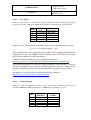
TABLE OF CONTENTS
1.
INSTRUMENT CHARACTERISTICS ...................................................................8
1.1
OVERVIEW ...............................................................................................................8
1.1.1 Instrument description ..........................................................................................8
1.1.2 OSIRIS focal plane masks...................................................................................10
1.1.3 Observing modes ................................................................................................11
1.1.4 Main Characteristics ..........................................................................................12
1.1.5 Field obscuration and vignetting ........................................................................13
1.1.6 Field orientation and gap ...................................................................................13
1.1.7 Instrument overheads..........................................................................................14
1.1.8 Environmental conditions ...................................................................................14
1.2
DETECTORS ...........................................................................................................14
1.2.1 Description .........................................................................................................14
1.2.2 OSIRIS standard CCD operation modes ............................................................16
1.2.3 OSIRIS CCDs linearity / dark current level / cross-talk ....................................16
1.2.4 Quantum Efficiency ............................................................................................17
1.2.6 CCD windowing .................................................................................................18
2.
BROAD BAND IMAGING .....................................................................................19
2.1.1
Sloan broad band filters .....................................................................................19
2.1.1.1
2.1.1.2
2.1.1.3
2.1.1.4
Zero points ...............................................................................................................................21
Sky background ........................................................................................................................21
Colour corrections ....................................................................................................................22
OSIRIS/GTC Broad Band Imaging efficiency .........................................................................22
PHOTOMETRIC UNIFORMITY ..................................................................................23
SKY FLAT FIELDS...................................................................................................23
SLOAN PHOTOMETRIC STANDARDS ......................................................................23
2.2
2.3
2.4
3.
TUNABLE FILTER IMAGING .............................................................................24
3.1
OSIRIS TUNABLE FILTERS DESCRIPTION .............................................................24
3.1.1 Introduction to FabryPerot filters (FPFs) ..........................................................24
3.1.1.1
3.1.1.2
3.1.1.3
3.1.2
3.1.3
3.1.4
Performance of an ideal FPF ....................................................................................................24
Limitations ...............................................................................................................................26
Gap-scanning etalons ...............................................................................................................27
Charge shuffling .................................................................................................29
Order sorters ......................................................................................................29
OSIRIS TF Characteristics and Features ...........................................................29
3.1.4.1
3.1.4.2
Dimensions...............................................................................................................................31
Coatings ...................................................................................................................................31
OSIRIS FOV FOR TUNABLE FILTER IMAGING ......................................................32
OSIRIS TUNABLE FILTER AVAILABLE WIDTHS ....................................................34
ORDER SORTER FILTERS .......................................................................................35
CALIBRATING THE TF AND TUNING ACCURACY ...................................................36
3.2
3.3
3.4
3.5
3.5.1 Parallelism..........................................................................................................36
3.5.1.1 General considerations ......................................................................................36
3.5.1.2
3.5.1.3
3.5.2
TF parallelization procedure.....................................................................................................36
Lack of parallelism ...................................................................................................................37
Wavelength calibration.......................................................................................39
USER MANUAL
Code: Draft
3.5.2.1
3.5.2.2
Page: 5 of 98
Date: July 6, 2011
File: OSIRIS-USERMANUAL_V1.1
General considerations .............................................................................................................39
Calibration using the ICM ........................................................................................................40
3.5.3 Checking the calibration by using night sky emission lines ...............................41
3.5.4 Tuning accuracy .................................................................................................43
3.5.5 Tuning speed .......................................................................................................43
3.6
OBSERVING WITH OSIRIS TUNABLE FILTER ........................................................43
3.6.1 Tunable Filter vs. Spectroscopy .........................................................................43
3.6.2 Observing Strategies...........................................................................................44
3.6.2.1
Selecting off-band wavelengths................................................................................................45
3.6.2.1.1
Continuum subtraction.......................................................................................................45
3.6.2.2
Deblending lines.......................................................................................................................46
3.6.2.3
On-line FWHM selection .........................................................................................................47
3.6.2.4
Deciding target position and orientation...................................................................................48
3.6.2.5
Removing ghosts, cosmic rays and cosmetics ..........................................................................49
3.6.2.5.1
Field masking ....................................................................................................................51
3.6.2.5.2
Azimuthal dithering pattern ...............................................................................................51
3.6.2.5.3
TF tuning dithering pattern ................................................................................................51
3.6.2.6
Tunable tomography.................................................................................................................51
3.6.2.6.1
Technique ..........................................................................................................................51
3.6.2.7
Band synthesis technique .........................................................................................................52
3.6.2.7.1
Technique ..........................................................................................................................52
3.6.2.8
SUMMARY .............................................................................................................................53
3.6.2.8.1
Sources of instrumental photometric errors. ......................................................................53
3.6.2.8.2
Preparing an observation: a checklist.................................................................................54
SPECTROPHOTOMETRIC STANDARDS FOR TF FLUX CALIBRATION........................55
OSIRIS RTF GLOBAL EFFICIENCY ........................................................................55
POST-PROCESSING TF DATA ..................................................................................56
3.7
3.8
3.9
3.9.1
Calibration images .............................................................................................56
3.9.1.1
3.9.1.2
Bias...........................................................................................................................................56
Flat fields..................................................................................................................................56
3.9.2 Night-sky emission line rings ..............................................................................57
3.10
MEDIUM BAND IMAGING WITH TF ORDER SORTERS ............................................58
4.
LONG SLIT SPECTROSCOPY .............................................................................60
4.1
4.2
4.3
4.4
4.5
4.5.1
4.5.2
4.5.3
4.6
4.7
4.8
4.9
5
OBSERVING WITH OSIRIS .................................................................................75
5.1
5.2
6
ACQUISITION IN LONG-SLIT SPECTROSCOPIC MODE.............................................61
FLEXURE................................................................................................................62
FRINGING ...............................................................................................................62
SPATIAL DISPLACEMENT .......................................................................................63
ARC LINE MAPS......................................................................................................64
Arc-line ghosts ....................................................................................................71
Spectral solutions ...............................................................................................71
Spectral flat fields ...............................................................................................72
VPHS R2000/R2500 GHOSTING ............................................................................72
SECOND ORDER CONTAMINATION .........................................................................73
SPECTROPHOTOMETRIC STANDARDS ....................................................................73
SPECTROSCOPIC PHOTON DETECTION EFFICIENCY ................................................74
EXPOSURE TIME CALCULATOR (ETC) ...................................................................75
GTC PHASE 2 TOOL ...............................................................................................75
OSIRIS DATA PROCESSING ...............................................................................76
USER MANUAL
Code: Draft
Page: 6 of 98
Date: July 6, 2011
File: OSIRIS-USERMANUAL_V1.1
6.1 OSIRIS / GTC KEYWORDS ...........................................................................................76
6.2 ASTROMETRY WITH OSIRIS .........................................................................................81
6.2.1
INPUT DATA ..........................................................................................................81
6.2.2
ASTROMETRIC SOLUTION ......................................................................................82
6.2.3
MOSAIC COMPOSITION ..........................................................................................84
6.2.4
COMPOSING A FIRST-ORDER MOSAIC FROM RAW DATA .......................................85
7
OSIRIS OS FILTER CHARACTERISTICS ........................................................86
8
OSIRIS GRISMS/VPH EFFICIENCIES ...............................................................91
9
SLOAN PHOTOMETRIC STANDARDS .............................................................94
10
OSIRIS SPECTROPHOTOMETRIC STANDARDS ..........................................96
A.
LIST OF REFERENCE DOCUMENTS ................................................................98
B.
REFERENCES .........................................................................................................98
USER MANUAL
Code: Draft
Page: 7 of 98
Date: July 6, 2011
File: OSIRIS-USERMANUAL_V1.1
LIST OF ABBREVIATIONS
AAO
Anglo Australian Observatory
CCD
Charge Coupled Device
ESAC/INSA
European Science Astronomy Centre / Ingeniería y Servicios Aeroespaciales
ESO
European Southern Observatory
EW
Equivalent Width
FITS
Flexible Image Transport System
FOV
Field Of View
FWHM
Full Width at Half Maximum
GTC
Gran Telescopio Canarias
IAA
Instituto de Astrofísica de Andalucía
IA-UNAM
Instituto de Astronomía – Universidad Nacional Autónoma de México
ICM
Instrument Calibration Module
IDT
Instrument Definition Team
IFCA-UNICAN Instituto de Física de Cantabria – Universidad de Cantabria
MOS
Multiple Object Spectroscopy
NIR
Near InfraRed
OSIRIS
Optical System for Imaging and low Resolution Integrated Spectroscopy
OS
Order Sorter
PI
Principal Investigator
PSF
Point Spread Function
QE
Quantum Efficiency
S/N
Signal to Noise ratio
TBC
To Be Confirmed
TBD
To Be Defined
TF
Tunable Filter
z
Redshift
USER MANUAL
Code: Draft
Page: 8 of 98
Date: July 6, 2011
File: OSIRIS-USERMANUAL_V1.1
1. INSTRUMENT CHARACTERISTICS
1.1
1.1.1
Overview
Instrument description
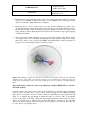
OSIRIS is the first work-horse imaging and spectroscopic instrument for the GTC. The
OSIRIS acronym stands for Optical System for Imaging and low-intermediate Resolution
Integrated Spectroscopy, which encapsulated in a few words the versatile nature of this
instrument that we will describe in this manual.
A key scientific driver in the design of OSIRIS has been the study of star formation
indicators in nearby galaxies and more distant objects, back to the furthest observable
galaxies with GTC. In particular, star formation in galaxies as a function of redshift is a
classical topic and one main objectives of several current projects of instruments for large
telescopes both, ground based and aboard satellites.
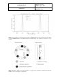
Figure 1.1.- 3D of OSIRIS showing the main subsystems.
USER MANUAL
Code: Draft
Page: 9 of 98
Date: July 6, 2011
File: OSIRIS-USERMANUAL_V1.1
OSIRIS is directly attached to the GTC field rotator and guide unit in the GTC Nasmyth-B
focal station (Figure 1.1). The instrument optics are designed around the classical concept of
collimator plus camera. For reasons of keeping the instrument compact, the optical train is
folded and the field is off-axis. Its compact design will allow future migration of the
instrument to the Cassegrain focal station. Next we will briefly describe the main
components of the instrument, following the light path from the moment the light coming
from the telescope enters the instrument through a transparent entrance window.
A masks loader (Figure 1.1) selects and insert/remove masks to/from the telescope focal
plane. In addition to user customized masks for multi-object spectroscopy, a number of fixed
width long-slit masks are available, as well as a number of special masks to facilitate fast
photometry and charge shuffling (see 1.1.2).
Having passed the focal plane, the light reflects of the collimator (Figure 1.1), which is an
off-axis quasi-parabolic mirror with elements for support and adjustment. The collimator is
open-loop actively controlled to compensate for gravitational flexures of the instrument
(Figure 1.1).
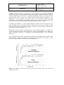
The collimated beam next hits a flat fold mirror that directs the light beam towards the filter
wheels and the camera optics. Both the collimator and folder are covered with a silver
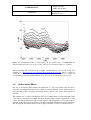
protected coating of high red and blue reflectivity (Figure 1.2).
Figure 1.2.- Collimator and folder flat measured reflectivity (curve) with respect to the requirements
(straight stepper lines)
USER MANUAL
Code: Draft
Page: 10 of 98
Date: July 6, 2011
File: OSIRIS-USERMANUAL_V1.1
Filters, grisms and Tunable Filters (TFs) can be inserted in the collimated beam near the
pupil via four filters wheels, three for standard filters and the fourth, at the pupil, for TFs and
grisms. Each filter wheel has 9 positions, and the grism wheel holds, apart from the tunable
filters, up to 5 dispersive element. Together they allow selecting the adequate combination of
these elements for using the different observing modes described in the following subsection.
Conventional filters are used for imaging and for order sorting the TFs and grisms. The filters
insert into the beam at an angle of 10.5 degrees in order to avoid ghost images.
The all-refractive OSIRIS camera consists of 9 spherical lenses. The last lens is the dewar
window. The camera effective focal length of 181 mm provides the required detector scale
(0.125 arcsec/pixel) on a flat focal plane that is tilted 1.83 degrees. The shutter is
incorporated in between the camera optics.
Light is detected by a mosaic of two detector of 2k×4k red-optimized CCDs in a cryostat
The instrument control subsystem allows mechanisms, tunable filters and the detector to
work in a synchronized fashion. Also, it provide users with mechanisms controls and data
processing interfaces. This instrument control is be closely integrated with the rest of
Telescope Control following the GTC standards. This facilitates a high level of automation of
observing sequences.
OSIRIS calibration is performed using spectral lamps provided by the GTC Instrument
Calibration Module (ICM), also, external continuum lamps for dome flat fields are available
at the telescope.
1.1.2
OSIRIS focal plane masks
The OSIRIS mask holder with 13 positions allows remote changes of focal plane masks such
as spectrograph slits, custom-made multi-object masks, or other special-purpose masks. The
following masks are available at the instrument:
•
Long Slit masks. Available slit widths are: 0.4", 0.6", 0.8", 1.0", 1.2", 1.5", 1.8", 2.0",
2.5", 3.0", 5.0".
•
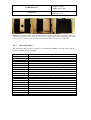
Decentred long slit of 3” width for fast photometry in shuffle mode (Figure 1.3 right).
•
Mask of the central 1/3 imaging FOV for TF imaging shuffle (two TF tunings or
straddling line, Figure 1.3 middle).
•
Frame transfer mask, selecting ½ of the lines in both detectors (Figure 1.3 left).
•
Mask shading one detector, for avoiding dithering when obtaining TF imaging of bright
crowded or extended fields.
•
Pinhole masks (for Long Slit and Multi Object Spectroscopy tests).
USER MANUAL
Code: Draft
Page: 11 of 98
Date: July 6, 2011
File: OSIRIS-USERMANUAL_V1.1
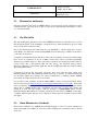
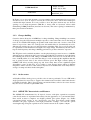
Figure 1.3.- From left to right, charge shuffling mask selecting the central 1/3 of the detector lines (the
central black circular piece is shown just for reference), frame transfer mask selecting the half of the
detector exposed, and the fast photometry mask with the decentred slit of 3 arcseconds width.
1.1.3
Observing modes
The following table provides a summary of the different OSIRIS observing modes, that are
described further on in this manual.
Mode
Imaging
Broad band
Narrow band
Single exposure
Scan
Shuffle
Spectroscopy
Long slit
MOS
Standard
λ-sorting
Nod & Shuffle
Standard
Microshuffle
λ-sorting
Fast photometry
Shuffle
Frame transfer
Fast Spectroscopy
Shuffle
Frame transfer
Description
SDSS and order sorter sets
With Tunable Filters: Blue (365-686 nm) and Red (646-1000 nm) TF
One wavelength for line and another for continuum
A set of exposures at several equidistant & contiguous wavelengths
Several wavelengths synchronizing charge shuffling with TF tuning
Slit widths defined by available masks
Using user-customized masks
Slitlets: sky and object in the same slit
As above but restricting wavelength range using a filter
Microslits: alternate sky & object by nodding telescope & shuffling
Charge is shuffled 1/3 of detector
As above but shuffling tens of rows instead
As any of the above but restricting wavelength range using a filter
Decentered slit plus charge shuffling
Defining windows and combining with frame transfer
Customized decentered and rotated 90º short slit
Off centre slit plus frame transfer on the detector
USER MANUAL
Code: Draft
1.1.4
Page: 12 of 98
Date: July 6, 2011
File: OSIRIS-USERMANUAL_V1.1
Main Characteristics
The following table summarises the main instrument characteristics.
Total FOV
8.53 × 8.67 arcminutes with small shadowed area in one side (Figure
1.4)
Unvignetted FOV
7.8 × 7.8 arcminutes
Long slit
8.67 arcminutes
MOS FOV
8.67 × 6.0 arcminutes1
Plate scale
0.12718 arcsec/pixel (both imaging and spectroscopy)
Image quality
< 0.15” (80% polychromatic EE)
Distortion
Lower than 2%
Instrument Position 150.540346º
Angle
Detector system
Two MAT 4k × 2k (∼9.2 arcsec gap2) from same Si wafer
Broad band
ugriz filters & medium band TF order sorters (OS)
Central λ tunable from 365 through 1000 nm3
FWHM tunable from ∼6 through ∼20 Å, depending on λ
Lower FWHM is limited by the order-sorting filter, and the higher by
Tunable Filters
the etalon gap range.
Tuning time ~10 ms depending on etalon gap. Minimum is ∼1 ms
Tuning accuracy in λ and FWHM ~1 Å
300, 500, 1.000, 2.000, 2.500 and 5.0004
Resolution for 0.6” slit width
Spectral resolutions
Available spectral ranges R=300 & 500 are limited by second-order
light, and higher R by detector5
Long slit widths
Masks of fixed widths from 0.4 through 5.0 arcseconds
∼40 targets per mask (using classical slits of 15” length) or
MOS (masks)
Several hundred (using Nod&Shuffle, µShuffle or λ-sorting)
Flexures
Less than 1 pixel
1
At R larger than 500, a 5 × 6 arcminute FOV is recommended.
2
Physical gap is of ∼26 pixels (or ∼3 arcsec), the gap between photosensitive pixels is of ∼72 pixels or
9.2 arcsec. Then, the last quantity is the one to take into account when dithering for covering the gap
on the sky.
3
Current IAC calibration facilities allow calibration from 450 through 950 nm only. In the near future
it will be expanded for covering the full OSIRIS wavelength range.
4
5
R=5000 VPHs are in manufacturing process.
Dispersive elements (grisms or VPHs) can be rotated 90º for accommodating the spectra along lines
or columns. The nominal dispersion direction is along columns (i.e.: along the gap between detectors).
Beware of detector gap if rotating the disperser.
USER MANUAL
Code: Draft
1.1.5
Page: 13 of 98
Date: July 6, 2011
File: OSIRIS-USERMANUAL_V1.1
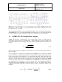
Field obscuration and vignetting
As can be appreciated from Figure 1.4, there is an obscuration of the left hand side OSIRIS
full FOV of CCD1 due to the edges of the filter wheels and the fold mirror. This was
contemplated in the original design and does not affect the specified unvignetted field of
view. The obscured area is best avoided, although reliable photometry can be performed on
targets located in this region of the detector.
Some vignetting is present in the lower part (lower 500 pixels, unbinned) of the
CCDs, due to filter wheel 1. With the filter in position removed, the vignetting is
reduced in CCD1 only (Figure 1.4). In all cases the total unvignetted field of view is
7.8 × 7.8 arcmin.
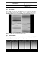
Figure 1.4.- OSIRIS image showing the shadowing produced by the folder flat and filter wheels on
one side of CCD1 (left). Since the instrument is off-axis, the centre of the OSIRIS field (10) does not
coincide with GTC pointing centre (in red).
1.1.6
Field orientation and gap
The OSIRIS instrument position angle within the GTC reference system is 150.540346º.
With this orientation, North is up and East left in the images. This value can be retrieved
from KEYWORD IPA at image headers. If a different position angle (P.A.) is requested by
the user, the resultant IPA would be 150.540346º - P.A. (with P.A. measured from N to E).
Page: 14 of 98
USER MANUAL
Date: July 6, 2011
File: OSIRIS-USERMANUAL_V1.1
Code: Draft
The OSIRIS focal plane is imaged by two CCDs that have a narrow gap between them. This
gap is 9.2 arcsecs wide. To cover the full field when defining a dithering pattern, steps of 10
arcsecs (or even 12 arcsecs to be more conservative) perpendicular to the gap are
recommended.
1.1.7
Instrument overheads
During instrument design, special efforts have been invested in reducing instrument
overheads due to configuration changes (observing modes, masks, and filters or grisms) to
the minimum. The following table summarizes the typical time it takes to change a
component.
Mask change
40 sec
Filter Change
3 sec
Grism Change
6 sec
These times only reflect the mechanical changes of the components and not the overheads for
target acquisition in the different modes, auto-guiding and detector readout.
Changing form one TF to the other takes about 13s. Changing TF wavelength tuning takes at
most about 0.1 s, usually 0.02 s, depending on the gap differences between the different
tunings.
1.1.8
Environmental conditions
OSIRIS is protected from the environment through its fairly air tight enclosure. Dry air
flushes the instrument to avoid dust and moisture entering the instrument and depositing on
optical surfaces. This air is provided by GTC instrument services and it is not thermally
controlled, but its temperature is quite stable. The aim is to minimize temperature and
humidity gradients within the instrument so as to ensure best image stability. Even when
inside the dome the humidity raises substantially due to wheather conditions, the humidity
inside OSIRIS is kept stable during several hours.
Temperature changes in GTC structure are transmitted quite fast by conduction to OSIRIS
structure via the Nasmyth flange to the GTC rotator. Also, although the attached electronic
cabinets are thermally isolated, some heat leaks inside the instrument.
1.2
1.2.1
Detectors
Description
The OSIRIS detector system is composed of a mosaic of two buttable 2Kx4K CCDs to give a
total 4Kx4K pixels, 15 microns/pixel. The arrays are MAT-44-82 from Marconi (2 channel
each, Frame-Transfer type, 20-1000 kHz readout rate). The software allows driving one or
both MAT44-82 CCDs, by one or two outputs each. It is also possible to modify the parallel
or serial clocks time, so that it is possible to readout the array from 20 kHz per channel up to
the CCD readout limit of 1 MHz. It allows frame transfer mode and binning.
Page: 15 of 98
USER MANUAL
Date: July 6, 2011
File: OSIRIS-USERMANUAL_V1.1
Code: Draft
The following table summarises the main OSIRIS detector parameters.
Parameter
Array size
Overscan area
Readout channels1
Shuffle speed
Readout speeds
RON3
Gain (e− /ADU)
Linearity
Operating Temp.
Dark current
CTE
Binning
Windows
Frame transfer
Fringing
Value
2048 × 4096
[1:24,1:2048]
2
50 µs/line
100, 200, 500 kHz
3.8 e− @ 100 kHz
4.5 e− @ 200 kHz
8 e− @ 500 kHz
1.18 @ 100 kHz
0.95 @ 200 kHz
Better than 1%
154-156 K
2-3 e− /hour/pixel
Vertical >0.999999
Horizontal >0.9999
2 × 1, 1 × 2 & 2 × 2
Up to 5 enabled
Enabled
3% @ 900nm
2% @ 950 nm
4% @ 990 nm
Comments
Photosensitive area
For bias subtraction
Per detector
Used for skipping lines in window mode as well
20,50kHz & 1 MHz possible (not recommended2)
Nominal are 200 kHz for imaging, 100 kHz for
spectroscopy & 500 kHz for acquisition
For 1% to 90% full well
Measured on grade 5 at laboratory
Nominal is 2 × 2
Copied on both detectors
For fast photometry & Spectroscopy
Fringing starts between 850 and 900 nm
Measured on grade 5 device at laboratory
1
Using two channel per detector requires obtaining all images in this configuration and slightly
different biases per channel (i.e.: half detector) are obtained
2
At 950 kHz the RON is so high that the image is not of scientific use, and at speeds lower than 100
kHz the readout time increases at a cost of no significant reduction of RON
3
RON @ 500 kHz is higher than nominal (∼8 e−), likely due to EMI (as of February 2010)
Readout times can be evaluated in the following way:
Pixels to read / (readout speed x binned pixels x channels used)
For example, reading both 2k × 4k full detectors using two channels per detector with 2 × 2
binning at 500 kHz takes ∼2 s.
Please note that this does not consider the time invested in configuring the SDSU (about 5s),
clearing the chip before each exposure (about 4s), and transferring and saving the frame on
disk (few more seconds).
Then, since an image is started till is fully acquired, for the two CCDs Output A and no
binning, takes 31 seconds at 500 kHz readout speed and about 100 s at 100 kHz.
Page: 16 of 98
USER MANUAL
Date: July 6, 2011
File: OSIRIS-USERMANUAL_V1.1
Code: Draft
1.2.2
OSIRIS standard CCD operation modes
As it was described in Section 1.2.1, the CCDs control system offers a wide range of readout
modes and gain settings, but for the time being the standard observing modes are shown in
the table below. In these modes the detector linearity is guaranteed up to the full 16 bits
signal maximum. Read noise is better than 5 electrons in imaging and spectroscopic readout
modes.
The acquisition mode is generally used for test images but not for science data. This mode
has a significant high noise pattern so it is not suitable for scientific cases. The following
table gives an overview of the main characteristics of the standard readout modes.
Imaging
(FAST)
Readout
configuration
Spectroscopy
(SLOW)
Acquisition
CCD1+CCD2_A CCD1+CCD2_A CCD1+CCD2_A
Readout velocity
200 kHz
100 kHz
500 kHz
Gain (e /ADU)
0.95
1.15
1.46
Binning (X x Y)
2x2
2x2
2x2
Readout time
21 sec
42 sec
-
-
-
2
Actual readout
noise
~4.5 e
~3.5 e
7.8 sec
~8 e-
A frequent monitorizing of the Gain and Readout noise for the standard operation modes of
OSIRIS is done for operational purposes, and the values are updated at the OSIRIS site at
GTC web page.
1.2.3
OSIRIS CCDs linearity / dark current level / cross-talk
In the OSIRIS standard operation modes, detector linearity is guaranteed up to the full 16 bits
signal maximum (Figure 1.5).
During the first months of operation of the instrument, OSIRIS suffered of a very high dark
current resulting from an excessive temperature of the CCD that was not correctly reported
by the CCD thermometry system. A redesign of the thermal coupling between the liquid
Nitrogen container and the CCD has resulted in a notable improvement of the dark current,
which is now at acceptable levels of about 10-12 ADUs/h for a 2 x 2 binned pixel. Hence,
since February 2010 no dark images are needed for OSIRIS data analysis.
2
Those values are for CCD2. Gain for CCD1 is about 5% lower that these.
USER MANUAL
Code: Draft
Page: 17 of 98
Date: July 6, 2011
File: OSIRIS-USERMANUAL_V1.1
A slight cross-talk effect between both CCDs in OSIRIS has been measured during
instrument commissioning tests. The effect is as small as 2.8 x 10-4 respect to the original
signal, hence the effect in the scientific images can be neglected.
Fig. 1.5.- : Linearity plots for OSIRIS SLOW (left) and FAST (right) operation modes.
Cosmic ray events have been measured in both OSIRIS CCDs, resulting an average of
30 impacts/min, that means around 1800 impacts/h.
1.2.4
Quantum Efficiency
The detectors are optimized for longer wavelengths, but with a low, although reasonable,
blue efficiency, of about 20% @ 365nm. Hence observing at these wavelengths is possible,
although slow.
Figure 1.6.-: QE of OSIRIS CCDs.
USER MANUAL
Code: Draft
1.2.6
Page: 18 of 98
Date: July 6, 2011
File: OSIRIS-USERMANUAL_V1.1
CCD windowing
OSIRIS CCDs allows to define up to 5 windows at the same time for SIMPLE readout
modes, and only a single window for FAST MODES (not available yet).
There are some restrictions that the user has to take into account when defining those
windows:
•
All the windows must have the same size.
•
No overlap is allowed between different windows.
•
Windows must be defined in increasing order of their Y coordinate (that coincides with
the readout direction). Therefore, Y coordinates for different windows must not overlap
(for example, if a window is defined at [1:200,300:499], any other window must begin at
Y=500, or conclude at Y=299).
•
Windows are replicated in both CCDs. Hence, if N windows are defined in CCD1, the
same windows will appear in CCD2, with the same size and position as those of CCD1.
Some cross-talk has been noted between windows in both CCDs, for this reason is highly
recommended that only use a single CCD when using windowing in OSIRIS.
The readout speed in windowing mode is defined by the combination of the windows size
and CCD readout mode. When windows are read out, the CCD section unused is ‘split’ at the
highest readout speed, hence there is no dependence in the total readout time on the windows
location in the CCDs.
In any case, if the user is interested in observing with OSIRIS by using windows, please
contact well in advance a GTC staff astronomer, in order to choose what is the most
convenient setup for the observing program. At the telescope, the GTC staff astronomer will
perform the observations, and all the restrictions and particularities in using the windows will
be properly considered.
Page: 19 of 98
USER MANUAL
Date: July 6, 2011
File: OSIRIS-USERMANUAL_V1.1
Code: Draft
2. BROAD BAND IMAGING
OSIRIS allows broadband imaging over a FOV of 8.53' x 8.67' (7.8’ x 7.8’ unvignetted)
covering the full spectral range from λ=3650 Å to λ=10000 Å , with a high transmission
coefficient in particular at longer wavelengths.
All standard OSIRIS filters have been designed to work in a collimated beam with a tilt angle
of 10.5º to avoid ghosts due to back reflections into the detector.
The OSIRIS standard pointing in Broad Band imaging mode is at the CCD2 pixel
(512,2048)3 to maximize the available FOV and in order to avoid possible cosmetic effects,
which are more abundant in the CCD1. The coordinates introduced by the PI in the Phase-2
tool will be positioned at this central pixel.
2.1.1
Sloan broad band filters
Broad band imaging with OSIRIS covers a spectral range from λ=3650Å to λ=10000 Å
using the standard Sloan filters u’(λ3500/600), g’(λ4750/1400), r’(λ6250/1400),
i’(λ7700/1500) and z’(λ9100/120).
The following table provides the measured parameters at the IAC optical laboratory at
ambient temperature at the centre of the filter and with normal incidence. Due to IAC
Laboratory limitations, no measures for u’ filter are available aside from those provided by
the manufacturer.
Filter
u’
g’
r’
i’
z’
Central wavelength
(Å)

4815
6410
7705
9695
FWHM
(Å)

1530
1760
1510
2610
Transmission
(%)

82.48
94.14
89.00
97.16
The filters are placed in the collimated beam and close to the pupil of the instrument, at an
angle of 10.5º with respect to the optical axis of the instrument. Because of the angle the
central wavelength [λc(10º)] is shifted with respect to the nominal central wavelength [λc(0º)]
and the bandwidth [∆λ] changes slightly, but the transmission curve shape is hardly altered.
Furthermore, depending on the location in the focal plane, the light incident on the filter
cover a range of angles between -2º y 22º, with the corresponding shift in
3
Note that those coordinates are unbinned coordinates, whereas the standard operation mode of OSIRIS implies
2 x 2 binning.
Page: 20 of 98
USER MANUAL
Date: July 6, 2011
File: OSIRIS-USERMANUAL_V1.1
Code: Draft
wavelength. For the broad-band filters this effect is small as can be seen in the
following table.
The maximum spatial variations of the filters with respect to the centre are:
Filter
u’
g’
r’
i’
z’
Central wavelength
(Å)

30
30
5
0
FWHM
(Å)

40
40
10
0
Transmission
(%)

1.05
1.36
1.09
1.39
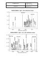
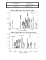
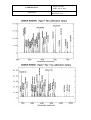
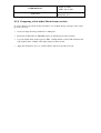
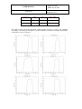
The absolute spectral responses for each filter (except u’) are provided in Figure 2.1.
Figure 2.1.- From left to right and top to bottom: measured central spectral response of g’, r, i’, and z’
filters, respectively, with normal incidence.
USER MANUAL
Date: July 6, 2011
File: OSIRIS-USERMANUAL_V1.1
Code: Draft
2.1.1.1
Page: 21 of 98
Zero points
From the observation of standard stars during instrument commissioning the following
average zero points (1 ADU/s at AM=0) and extinction coefficients have been measured:
Filter
u’
g’
r’
i’
z’
Zero point
Extinction
(mag)
(mag/airmass)
25.84(±0.08)
0.44(±0.01)
28.85(±0.05)
0.14(±0.03)
29.31(±0.06)
0.07(±0.03)
28.86(±0.05)
0.02(±0.07)
28.27(±0.07)
0.05(±0.02)
With those zeropoints, instrumental magnitudes can be obtained directly using the formula:
m = Z – 2.5 log10 [Flux (ADUs/s)] – k X
The zeropoints have been measured at the standard GTC pointing for Broad Band
imaging (that is placed at OSIRIS CCD2). Zeropoint values for CCD1 are on average
0.1-0.12 mag smaller in each filter than these.
Standard extinction coefficients for the ORM can be found at:
http://www.ing.iac.es/Astronomy/observing/manuals/ps/tech_notes/tn031.pdf
The limiting magnitudes are measured during photometric sky conditions. Clouds or
dust in the atmosphere will reduce the limiting magnitudes. Likewise, changes in the
cleanliness and transmission of all optical components will affect the zero points.
An updated version of the daily zeropoint values can be found at:
http://www.gtc.iac.es/en/media/osiris/zeropoints.html
2.1.1.2
Sky background
Estimates of the sky brightness (ADUs /s/ pix) measured at a Elevation 55 deg in the
standard OSIRIS Broad Band imaging mode (200 kHz / 9.5 - binning 2 x 2) are:
Filter
u’
g’
r’
i’
z’
Sky Brightness Sky Brigthness
(BRIGHT)
(DARK)
15
1
250
25
350
90
290
160
400
325
Page: 22 of 98
USER MANUAL
Code: Draft
Date: July 6, 2011
File: OSIRIS-USERMANUAL_V1.1
Although ETC predictions for sky brightness at the ORM are accurate enough, it is
recommended to use the values from the table above for a quick estimation of the sky
background counts in long exposed images.
2.1.1.3
Colour corrections
Photometric transformations equations (with a arbitrary zero point of 25. magnitudes) are:
u’ – u’0 = -0.517(±0.053) - 0.071(±0.023) (u0 – g0)
g’ – g’0 = -3.637(±0.040) - 0.078(±0.013) (g0 – r0)
r’ – r’0 = -4.117(±0.017) - 0.114(±0.028) (r0 – i0)
i’ – i’0 = -3.170(±0.015) - 0.079 (±0.041) (i0 – z0)
z’ – z’0 = -3.310(±0.031) - 0.072 (±0.052) (i0 – z0)
2.1.1.4
OSIRIS/GTC Broad Band Imaging efficiency
The graph below shows the overall photon detection efficiency of GTC and OSIRIS in each
of the Sloan filters (the plots include the contribution both of the telescope and
instrument optics system).
Figure 2.3.- Overall photon detection efficiency of GTC and OSIRIS in each of the Sloan filters.
USER MANUAL
Code: Draft
2.2
Page: 23 of 98
Date: July 6, 2011
File: OSIRIS-USERMANUAL_V1.1
Photometric uniformity
Given the structure and speed of OSIRIS shutter (of type moving screen) and that it is near
collimated beam, exposures down to 0.1 seconds can be obtained with a uniformity of about
1% over the full field.
2.3
Sky Flat fields
The flat fielding homogeneity in each of the OSIRIS Sloan filters is better than 2.5% over the
full unvignetted FOV of the instrument, except in Sloan u', where fluctuations up to 6% with
respect to the mean value are found.
Day to day fluctuations in the flat fields are less than 0.05% , and less than 0.1% week to
week. Hence, sky flat fields obtained with OSIRIS are well usable up to within a week before
or after the observations.
Comparison twilight flat fields with those derived from scientific observations during bright
time shows no variations in excess of 0.01%, hence they can be considered practically
identical for scientific purposes. These percentage variations are measured globally, while of
course locally, due to dust particles that can come and go, the variations may be larger.
Moreover, differences between the night sky and the twilight spectrum may result in subtle
flat fielding differences.
Comparisons between fky flat fields and dome flats show that the latter suffer from
inhomogeneities in the dome illumination. Differences up to 10-15% are found in CCD2 and
2% in CCD1. Therefore dome flats are only recommended for obtaining reliable OSIRIS
photometry in CCD1 and as last choice in CCD2.
As a product of the scientific operations with OSIRIS, a series of master flat fields frames
can be retrieved from http://www.gtc.iac.es/en/pages/instrumentation/osiris.php. Flat fields
were all obtained with exposure times larger than 1 s to minimize possible photometric
effects due to OSIRIS shutter and a maximum exposure time of about 20 s (where the
detection of stars becomes notable), with an average of 35,000-40,000 ADUs in each
individual image. MasterFlats are available separately for each CCD of OSIRIS (as they have
a slightly different gain and bias level). The latest master flats are available from the GTC
web pages.
2.4
Sloan Photometric Standards
Photometric calibration for OSIRIS Broad Band imaging is done via a Sloan standard set
taken from Smith el al. (2002, AJ, 123, 2121). The complete list of standards can be found in
Section 9.
Page: 24 of 98
USER MANUAL
Date: July 6, 2011
File: OSIRIS-USERMANUAL_V1.1
Code: Draft
3. TUNABLE FILTER IMAGING
3.1
OSIRIS Tunable Filters description
A key aspect of OSIRIS is the use of tunable filters (TFs). OSIRIS TFs are a pair of tunable
narrowband interference filters (FabryPerot etalons) covering 370–670 nm (blue ‘arm’) and
651–935 nm (red ‘arm’). They offer monochromatic imaging with an adjustable passband of
between 0.6 and 3 nm. In addition, TF frequency switching can be synchronized with
movement of charge (charge shuffling or frame transfer) on the OSIRIS CCDs, techniques
that have important applications to many astrophysical problems.
3.1.1
Introduction to FabryPerot filters (FPFs)
In its simplest form, a FabryPerot filter (FPF) consists of two plane parallel transparent plates
which are coated with films of high reflectivity and low absorption. The coated surfaces are
separated by a small distance (typically µm to mm) to form a cavity which is resonant at
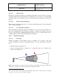
specific wavelengths. Light entering the cavity undergoes multiple reflections (Figure 3.1)
with the amplitude and phase of the resultant beams depending on the wavelength. At the
resonant wavelengths, the resultant reflected beam interferes constructively with the light
reflected from the first plate cavity boundary and all the incident energy, in the absence of
absorption, is transmitted. At other wavelengths, the FPF reflects almost all of the incident
energy.
3.1.1.1
Performance of an ideal FPF
The general equation for the intensity transmission coefficient of an ideal FPF (perfectly flat
plates used in a parallel beam) as a function of wavelength is
2
4R
 T  
 2πµd cosθ
τr = 
sin 2 
 1 +
2
λ
 1 − R   (1 − R )

−1

 ,

(3.1)
where T is the transmission coefficient of each coating (plate–cavity boundary), R is the
reflection coefficient , d is the plate separation, µ is the refractive index of the medium in the
cavity (usually air, µ =1) and θ is the angle of incident light. Thus, the FPF transmits a
narrow spectral band at a series of wavelengths given by
mλ = 2 µd cos θ
(3.2)
where m is an integer known as the order of interference. The peak transmission of each
passband is
2
τ r ,max
2
 T 
 T 
=
 =
 ,
1− R 
T + A
(3.3)
Page: 25 of 98
USER MANUAL
Date: July 6, 2011
File: OSIRIS-USERMANUAL_V1.1
Code: Draft
where A is the absorption and scattering coefficient of the coatings (A = 1 – T – R); and the
minimum transmission, halfway between the resonant wavelengths is
Therefore, the contrast between the maximum and minimum transmission intensities is
Cr =
τ r ,max  1 + R  2
=
 .
τ r ,min  1 − R 
(3.4)
For a FPF contrast greater than 100, the reflection coefficient R of the coatings needs to be
greater than or about 0.82.
The wavelenght spacing between passbands, known as the inter–order spacing or free
spectral range (FSR), is about
λ
∆λ =
(3.5)
m
which is obtained from Equation 3.2 by setting consecutive integral values of m. Each
passband has a bandwidth (δλ), full width at halfpeak transmission, given by
δλ r =
λ (1 − R )
mπR 1 / 2
(3.6)
derived from Equation 3.1. The ratio of inter–order spacing to bandwidth is called the
finesse;
N=
∆λ
δλ
.
(3.7)
2
τ r , min
 T 
=
 .
1 + R 
(3.8)
For an ideal FPF, it is given by
Nr =
∆λ
δλ r
=
πR 1 / 2
1− R
.
(3.9)
Thus, we can see that the resolving power of a FPF is equal to the product of the order and
the finesse;
λ
= mN .
δλ
(3.10)
USER MANUAL
Code: Draft
Page: 26 of 98
Date: July 6, 2011
File: OSIRIS-USERMANUAL_V1.1
Figure 3.1.- Schematic diagram of interference with a FabryPerot filter. The outside surfaces of the
glass are coated with antireflective (AR) coatings, while the inside surfaces are highly reflective
(usually R > 0.8). The air cavity in the middle is not shown to scale (usually, d is about 10 µm whereas
the glass is over 20 mm thick on both sides). At resonant wavelengths, the first reflection (shown with
a solid line) interferes destructively with light coming from the cavity in the same direction (dashed
lines). The phase difference arises because the first reflection is `internal', while all the other
reflections are `external' (with respect to glass). On the other side of the cavity, only constructive
interference occurs. At nonresonant wavelengths, destructive interference occurs in the cavity and the
first reflection dominates.
3.1.1.2
Limitations
It is apparent from the above equations that to obtain a higher resolution for a given order or
to obtain a wider interorder spacing for a given resolution, the finesse needs to be increased.
For a finesse greater than 100, a reflection coefficient R of greater than or about 0.97 is
necessary (Equation 3.9). However, so far we have considered the ideal situation where the
plates are flat and parallel, and the incoming light is parallel. In particular, Equations 3.1,
3.3–3.5, 3.7 and 3.9 refer to this situation using the subscript r to distinguish the results from
a real filter. In practice, plate defects and the angular size of the beam limit the maximum
finesse obtainable.
Page: 27 of 98
USER MANUAL
Date: July 6, 2011
File: OSIRIS-USERMANUAL_V1.1
Code: Draft
The effective finesse (N) is approximately given by:
1
1
1
1
= 2 + 2 + 2,
2
N
Nr Nd Na
(3.11)
where Nr is the reflective finesse from Equation 3.9, Nd is the defect finesse (due to plate
defects) and Na is the aperture finesse (due to the solid angle of the beam).
The defect finesse
Nd ~
2π
,
2δd
(3.12)
where δd is a length scale related to deviations from flat parallel plates. The exact details
depend on the type of deviations (Atherton et al. 1981). A FPF manufactured with Nd ∼ 80
and a reflection coefficient of 0.97 (Nr ∼ 100) performs with a finesse of about 60.
The aperture finesse
Na ~
2π
,
mΩ
(3.13)
where Ω is the solid angle of the cone of rays passing through the FPF. This equation is
related to the λ dependence on θ in Equation 3.2. In terms of astronomical imaging, the effect
of aperture finesse is negligible for most objects in the field of view of a telescope. For
example, an object which is one degree across (in the collimated beam) imaged with m =50
has Na ∼500 according to Equation 3.13. A more relevant analysis to consider the change in
central wavelength of the filter as the ray angle θ is varied in Equation 3.2. For example, a
change in ray angle from 1º to 3º produces a change of 0.1% in the central wavelength of the
filter at any given order. Therefore, at high resolving powers (∼1000), a FPF may not be truly
monochromatic across a desired field of view.
3.1.1.3
Gap-scanning etalons
In order to manufacture a tunable FPF, which can change the central wavelength for a given
order, it is necessary to be able to adjust either the refractive index of the cavityµ, the plate
separation d or the angle θ (as can clearly be seen from Equation 3.2). In a gap-scanning
etalon, the plate separation can be controlled to extremely high accuracy.
USER MANUAL
Code: Draft
Page: 28 of 98
Date: July 6, 2011
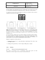
File: OSIRIS-USERMANUAL_V1.1
Figure 3.2.-: Variation of the transmission profile of a FPF with finesse. The profiles were determined
for an ideal FPF (Equation 2.25) with R = 0.68, 0.81 and 0.92 (A = 0). Orders m = 10 and m = 9 are
shown.
Figure 3.3: Front elevation and side elevation of a Queensgate Instruments etalon. Note that the
thickness of the optical gap is exaggerated.
USER MANUAL
Code: Draft
Page: 29 of 98
Date: July 6, 2011
File: OSIRIS-USERMANUAL_V1.1
In Figure 3.3, we show the structure of a gap-scanning etalon manufactured by Queensgate
Instruments Ltd. (now IC Optical Systems) In recent years, these etalons have undergone
considerable improvements. It is now possible to move the plates between any two discrete
spacings at very high frequencies (200 Hz or better) with no hysteresis effects while
maintaining λ/2000 parallelism (measured at 633 nm). The etalon spacing is maintained by
three piezoelectric transducers.
3.1.2
Charge shuffling
Central to almost all modes of OSIRIS use is charge shuffling. Charge shuffling is movement
of charge along the CCD between multiple exposures of the same frame, before the image is
read out. For shuffled TF imaging an aperture mask ensures that only a section of the CCD
frame is exposed at a time. For each exposure, the tunable filter is systematically moved to
different gap spacings in a process called frequency switching. This way, a region of sky can
be captured at several different wavelengths on a single image. Alternatively, the TF can be
kept at fixed frequency and charge shuffling performed to produce timeseries exposures.
The TF plates can be switched anywhere over the physical range at rates in excess of 100 Hz,
although in most applications, these rates rarely exceed 0.1 Hz. If a shutter is used, this limits
the switching rate to about 1 Hz. Charge on OSIRIS CCDs can be moved over the full area at
rates of 30-50 µs/line: it is only when the charge is read out through the amplifiers that this
rate is greatly slowed down to the selected readout speed. The high cosmetic quality of
OSIRIS CCD allows moving charge up and down many times before significant signal
degradation occurs. In this way, it is possible to form discrete images taken at different
frequencies where each area of the detector may have been shuffled into view many times to
average out temporal effects in the atmosphere.
3.1.3
Order sorters
A FabryPerot Filter clearly gives a periodic series of narrow passbands. To use a FPF with a
single passband, it is necessary to suppress the transmission from all the other bands that are
potentially detectable. This is done by using conventional filters, called order sorters because
they are used to select the required FPF order.
3.1.4
OSIRIS TF Characteristics and Features
The OSIRIS TF, manufactured by IC Optical Systems, with plate separations accurately
controlled by means of capacitance micrometry, has the appearance of a conventional FabryPerot etalon in that it comprises two highly polished glass plates (Figure 3.4). Unlike
conventional ICOS etalons, it also incorporates very large piezoelectric stacks (which
determine the plate separation) and high performance coatings over half the optical
wavelength range. The plate separation can be varied between about 3-4µm to 10 µm.
USER MANUAL
Code: Draft
Page: 30 of 98
Date: July 6, 2011
File: OSIRIS-USERMANUAL_V1.1
The highly polished plates are coated for optimal performance over 370–960 nm using two
separate etalons, one optimized for short wavelengths and one for longer wavelengths. The
coating reflectivity determines the shape and degree of order separation of the instrumental
profile. This is fully specified by the coating finesse, N, which has a quadratic dependence on
the coating reflectivity. The OSIRIS TF was coated to a finesse specification of N = 50 (red)
-100 (blue) which means that the separation between periodic profiles is, respectively, fiftyone hundred times the width of the instrumental profile. At such high values, the profile is
Lorentzian to a good approximation. For a given wavelength, changes in plate spacing, d,
correspond to different orders of interference, m. This in turn, dictates the resolving power
(mN) according to the finesse.
Figure 3.4.- OSIRIS red etalon at the IAC Optical Lab, while undergoing calibration tests.
In general, as can be appreciated in Eq. 3.2, for a given order, small changes in d change
slightly the wavelength, while for a given wavelength the change of order requires a larger
change in d. This is important to keep in mind.
Page: 31 of 98
USER MANUAL
Date: July 6, 2011
File: OSIRIS-USERMANUAL_V1.1
Code: Draft
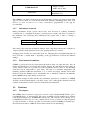
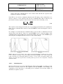
With very good approximation, the spectral response of a TF, given by eq. (3.1) can be
expressed by,
−1
  2(λ − λ 0 )  2 
T = 1 + 
  ,
  δλ
 
(3.14)
where λ0 is the wavelength at maximum transmission.
1,0
0,9
Transm iss ion
0,8
0,7
0,6
Tunable filter
Gaussian
0,5
0,4
0,3
0,2
0,1
0,0
0,56 5
0,570
0,5 75
Wavelength (m ic rons)
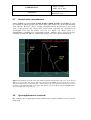
Figure 3.5.- Spectral response of a TF wrt. a Gaussian. The TF response can be considered Gaussian
with a good approximation above FHWM, but is more winged below FWHM. This has to be taken
into account when selecting the on and off frequencies.
3.1.4.1
Dimensions
The OSIRIS TF are model ET-100. Then the clear aperture is 100 mm diameter. The units
are approximately 170 mm diameter by 100 mm of thickness and have a weight of
approximately 8 kg.
3.1.4.2
Coatings
This is a critical aspect of TF performance as shown in section 3.1.1. For the OSIRIS TF the
main difficulty is achieving a relatively constant reflectivity for a wide spectral range: from
370 to 670nm for the blue TF and from 650 through 1000nm for the red TF. This implies
multilayered coatings, i.e.: thick coatings. Then the minimum distance (widest FWHM)
between plates is driven by the minimum distances between the coating surfaces, not the
plate surfaces.
Page: 32 of 98
USER MANUAL
Date: July 6, 2011
File: OSIRIS-USERMANUAL_V1.1
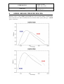
Code: Draft
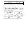
Figure 3.6.- Mean transmissions T for the blue (left) and red (right) OSIRIS TF. The mean
reflectivity R = 100 – T % with a very good approximation. This results in a mean R = 91% for the
blue TF and 94% for the red TF.
The wavelength dependence of the reflectivity R translates into a wavelength dependence of
the FWHM range. Also, please note that the R is well behaved above 425 nm for the blue TF
and above 650 nm for the red TF. Hence deviations are expected at lower wavelengths.
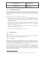
3.2
OSIRIS FOV for Tunable Filter Imaging
OSIRIS TF provides a circular FOV of 4 arcmin radius, where is assured that the
observations will not have any contamination of other interference orders in the filter. The
TF, as any interference filter, changes its response with the incident angle θ according to the
formula,
λθ =
λ0 n 2 − sin 2 θ
(3.15)
n
where λ0 is the central wavelength for normal incidence, λθ for the incident angle θ and n the
refraction index.
As a consequence, for filters in a collimated beam (OSIRIS case), beams from different
points of the GTC focal plane reach the TF at increasing incident angles, with symmetry with
respect to the optical centre. Then there is a progressively increasing shift to the blue of the
central wavelength as the distances r to the optical centre increase, according to Eq. 3.15.
However, since the beams coming from the same point of the FOV are parallel, the FWHM
is nearly the same. This is the case of OSIRIS, since OSIRIS TF are located in the pupil of
the collimated beam. Since this is a pure geometric effect, the wavelength variation is
completely fixed and predictable because it depends only on the incident angle, that is
completely determined by the ratio between the telescope and the instrument collimator focal
distances:

2
r

 
 
 arc min  
λ (r ) = λ 0 1 − 7.9520 ⋅ 10 − 4 

(3.16a)
USER MANUAL
Page: 33 of 98
Date: July 6, 2011
File: OSIRIS-USERMANUAL_V1.1
Code: Draft
Where r is obtained from the OSIRIS plate scale of 0.127 arcsec/pixel. This equation allows
obtaining an accuracy of ≈1-2Å at the edge of the 8 arcminute diameter TF FOV (that is the
worst case), depending on wavelength. This accuracy is enough for most purposes, since the
accuracy of the TF tuning is of ≈1-2Å. However, were more accuracy required, the following
full expression can be used instead:

f
λ (r ) = λ0  1 +  GTC

 f Coll


r 

2




−1
2

r 
−3 
= λ0  1 + 1.5904 ⋅ 10 

arcmin 







−1
(3.16b)
since the measured focal lengths are fGTC = 169888±2mm (Castro et al. 2007) and
fColl = 1240.90±0.05mm (SESO 2006), where wavelength or temperature variations can be
neglected.
The TF optical center is located at pixel (2118, 1966) of CCD1, including the 50 pixels of
overscan, within the gap of the CCDs, and 20 pixels away from the right edge of the CCD14.
The wavelength observed with the TF relative to this point changes following Eq (3.16).
Users should be aware that the wavelength tuning is not uniform over the full field of
view of OSIRIS.
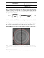
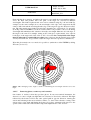
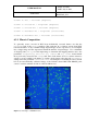
Figure 3.7.- Image with OSIRIS RTF tuned at 732.5 nm, showing the 4 arcmin radius where no
contamination from other interference orders is assured. This is the operative FOV of the OSIRIS
RTF.
4
Note that those coordinates are unbinned coordinates, whereas the standard operation mode OSIRIS implies
2 x 2 binning.
USER MANUAL
Code: Draft
Page: 34 of 98
Date: July 6, 2011
File: OSIRIS-USERMANUAL_V1.1
The position of the objects in the Tunable Filter observing mode depends on the requirements
of the PI since the value of the wavelength changes with the object's position in the FOV.
The PI must indicate, in the Phase-2 form, the coordinates to which the telescope will be
pointing and the CCD pixel position corresponding to these coordinates. By default, the
pointing will be done at 15 arcsecs from the optical center of the system, in the pixel (100,
1966) at the CCD25.
3.3
OSIRIS Tunable Filter available widths
When working with the OSIRIS tunable filters the user needs to take into account two
parameters: the observing wavelength and the required FWHM.
The range of operation of the OSIRIS Red Tunable Filter (the only available at the telescope)
is from 651 nm to 934.5 nm (this range will be increased in future upgrades of the
instrument).
It should also be noted that the practical use of the Red Tunable Filter is more restrictive than
was originally anticipated. The minimum width achievable is 1.2 nm, that is imposed by the
design of the order-sorting filters, in order to avoid contamination by other interference
orders within the FOV. There is also a maximum width, depending on the wavelength range,
as follows:
•
2.0 nm for λ < 800 nm
•
1.5 nm for 800 nm < λ < 850 nm
•
1.2 nm for λ > 850 nm
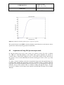
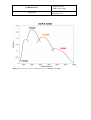
In addition to the information of the maximum tunable widths with the TFs as a function of
wavelength (see table above) Figure 3.8 shows the available range of widths as a function of
wavelength. The minimum width is 1.2 nm for all the wavelength to avoid contamination due
to other orders in a circular FOV of 4 arcmin radius (this value is also the maximum usable
width for wavelengths longwards of 850 nm).
5
Note that coordinates are unbinned coordinates, whereas the standard operation mode of OSIRIS implies 2 x 2
binning.
USER MANUAL
Code: Draft
Page: 35 of 98
Date: July 6, 2011
File: OSIRIS-USERMANUAL_V1.1
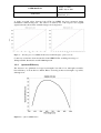
Figure 3.8.- Available TF widths vs wavelength for all the operative range of OSIRIS RTF. The
minimun width achievable is shown as a red line, that is also the maximum width for λ > 850 nm.
When preparing TF observations it is highly recommended to use the TF Setup Tool
available at: http://www.gtc.iac.es/en/pages/instrumentation/osiris.php. This tool allows to
obtain the available widths for our wavelength of interest, as well as to define the
corresponding Order Sorter Filter that has to be used for the observation (see Section 7).
3.4
Order Sorter Filters
The use of the tunable filters implies the utilization of order sorter filters (OS) in order to
select the wavelength band that avoids confusion between different orders of interference of
the Fabry-Perot. The observing wavelength defines which order shorter filter should be
selected.
The available set of order sorter filters provides for a suitable filter for all wavelengths. Order
sorter filters overlap in wavelength, but their working range ensures suppression of other
orders. The OS are tilted 10.5 degrees with respect to TF and grisms, to avoid ghosts due to
backwards reflections from the detector (the TF is not tilted and therefore suffers reflections.
The description and characteristics for the complete OS filter set can be found in Section 7.
USER MANUAL
Code: Draft
3.5
3.5.1
Page: 36 of 98
Date: July 6, 2011
File: OSIRIS-USERMANUAL_V1.1
Calibrating the TF and Tuning accuracy
Parallelism
3.5.1.1 General considerations
TF parallelization consist in determining the X and Y values that keep plates parallel, and
depends on Z and λ. OSIRIS TF Parallelism is very robust, and does not vary with time even
when switching off and on again the TF controller. Hence, once the XY values for a certain Z
and λ range are determined, they can be used around these Z and λ values from then on.
Checking parallelism values from time to time is recommendable.
3.5.1.2
TF parallelization procedure
This parallelisation procedure for the TF is a task to be done during the day. The basis
consists of maximizing the intensity of the light in the optical centre of the TF, when tuned to
the wavelength of an emission line from a calibration lamp, while varying X and Y. This is
the same procedure to be employed for wavelength calibration, but then varying Z. A lack of
parallelism (XY) or a poor of wavelength tuning (Z) will reduce the intensity measured. This
procedure is achieved by inserting a wide centred long slit, and stepping the charge on the
CCD while varying X, Y or Z in a systematic fashion. The TF must be tuned to the
wavelength of an emission line (i.e.: the Z must be the one corresponding to the emission
line)
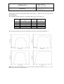
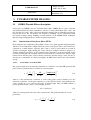
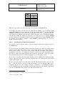
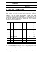
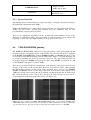
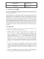
Figure 3.9.- Example of a X calibration image of 14 steps of 50 bits. Seen in the image is a slit
illuminated by an arc lamp. The slit is centered on the field. After each exposure the charge is shifted
downwards, the X setting of the TF changed, and a new image of the slit is taken. After a sequence of
USER MANUAL
Code: Draft
Page: 37 of 98
Date: July 6, 2011
File: OSIRIS-USERMANUAL_V1.1
several steps the CCD is read out, which results in a series of slit images as is shown here. N note that
in the X calibration, the slit image intensities are not symmetric.
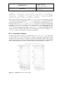
Figure 3.10.- Example of a Y calibration image of 8 steps of 25 bits.. Note that in the Y calibration,
the slit image intensities are not symmetric.
3.5.1.3
Lack of parallelism
If the TF plates are not parallel the result will be:
•
Distorted rings of the night sky emission lines and of calibration lamp lines.
•
Asymmetric wavelength calibration (Z) scans, that are in opposite directions depending
whether there is an excess or lack in X or Y values (see figure 3.11)
•
Lower intensities of slit images in wavelength calibration (Z) scans
•
Wavelength shifts
The main consequences for the data are:
•
Transmission losses
•
Wider FWHM and distorted spectral response
Page: 38 of 98
USER MANUAL
Date: July 6, 2011
File: OSIRIS-USERMANUAL_V1.1
Code: Draft
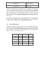
The XY resolutions used for parallelism calibration, 50 and 25 bits, respectively, have been
chosen as the most convenient. Larger steps are not accurate enough and the XY errors affect
wavelength and transmission as shown in the following table (approximate values to serve as
example only) for the red TF.
± errors
Red TF
∆X=±50
∆Y=±25
λ shift
(nm)
0.1
0.1
0.3
0.2
δT/T
(%)
4
4
3
0
It is important to keep a good parallelism better than 50 bits in X and 25 in Y. Again, note
that Y is more sensitive.
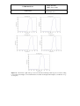
Figure 3.11.- Example of intensity losses and resulting asymmetric slit image intensity profiles
obtained for the same Z calibration scan, in the following situations: top-left using Xbest+50 the Z
scan is asymmetric and concave below the maximum intensity. Top-right using Xbest−50 the Z scan is
asymmetric and concave above the maximum intensity. Bottom-left using Ybest+25 the Z scan is
asymmetric and concave above the maximum intensity. Bottom-right using Ybest−25 the Z scan is
asymmetric and concave below the maximum intensity.
USER MANUAL
Code: Draft
3.5.2
3.5.2.1
Page: 39 of 98
Date: July 6, 2011
File: OSIRIS-USERMANUAL_V1.1
Wavelength calibration
General considerations
Parallelization is a day-time procedure, because it is very stable in time and even with
temperature changes and instrument rotation. Wavelength calibration, on the other hand, is a
nightly procedure, since the Z-λ calibration depends upon many factors, and the calibration
must be checked during the night, even for the same wavelength and order.
The wavelength calibration consists of establishing the relation between Z values in bits and
the wavelength. This relation is non-linear enough, so that a linear approximation can be
deemed valid only locally. Through tests of the TF carried out under controlled
environmental conditions the relation between Z and wavelength has been derived for every
order and through the full wavelength range that each TF can cover.
Extensive tests show that The λ-Z curve may be offset in Z by a constant factor, depending
on the environmental conditions with a precision of 5 bits in Z (i.e.: better than 0.1nm).
However, it is necessary to determine the offset for Z mimicking as closely as possible the
true observing conditions. So in essence, wavelength calibrating the TF consists of
determining this offset. This is done at the telescope by using a calibration lamp of the ICM.
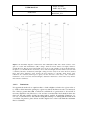
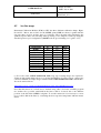
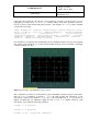
Figure 3.12.- Z calibration scan. 20 slit images can be seen. The first one is the bottom one. The
tuning lies between image 11 and 12 as can be appreciated both from the maximum intensity and
symmetry. Non symmetric intensities are suspicious of lack of parallelism.
USER MANUAL
Code: Draft
3.5.2.2
Page: 40 of 98
Date: July 6, 2011
File: OSIRIS-USERMANUAL_V1.1
Calibration using the ICM
The calibration procedure using the ICM has already been described within the
parallelization procedure of the previous section. An accurate wavelength calibration can be
obtained only after parallelization, i.e.: determining the best XY values for the given range of
Z and wavelength.
Wavelength calibration depends, at least, of the following:
•
Humidity. This is potentially an important factor, but since the instrument is flushed with
dry air6 its effect is for practical purposes insignificant.
•
Temperature. This produces a highly non-linear effect where the etalon undergoes
several phases of different variations. ET100 are quite large and take up to three hours to
stabilize versus temperature changes. However this is not as serious as it seems, since
implies only calibrating more frequently, depending on the history and the temperature
gradient. It has been demonstrated to be safe operating with TF temperature gradients of
at least 0.6ºC/hour, produced by temperature differences between TF and telescope of
several degrees, as long as calibration is checked every 20 or 30 minutes. When the
temperature gradient is of the order of 0.1-0.2 ºC/hour the tuning can be considered
stable for at least one hour. Telescope gradients are normally far smaller In the future the
instrument control system will take care of this effect at user’s request.
•
Instrument rotator angle. The calibration of the TF is highly dependent on the angle of
the rotator, and hence on the orientation of the TF. We can find differences of up to 40
bits (~8A) between two rotator positions (see fig below). In order to avoid this we define
for TF operation the following useful range (-160° < θ < -40º and 50º < θ <160º). This
range ensures a stable calibration accuracy of ±0.1nm and, if the rotator is moving less
than 10°, the calibration can be considered virtually unchanged, with the precision given
by the self-calibration (± 0.02nm = 1 bit).
During the normal operation the observer predicts in advance, using the coordinates of
the object and its instrument position angle, the position of the rotator to a specific time
in order to ensure that the observations are performed in the useful range.
This variation is independent both of wavelength and distance between plates (Z).
•
TF history: if plates collide, the TF calibration might change. This is unlikely to happen
since the Z range has been limited to safe values.
6
However, caution must be taken when opening the instrument for changing filters or masks shortly before
observations. See environmental conditions in user manual.
Page: 41 of 98
USER MANUAL
Date: July 6, 2011
File: OSIRIS-USERMANUAL_V1.1
Code: Draft
Figure 3.13.- Variation of the TF tuning (Z) with the rotator angle.
All those factors produce day to day variations in the TF calibration. For this reason the TF
has to be calibrated before every observing block.
3.5.3
Checking the calibration by using night sky emission lines
The OH group produce relatively strong emission lines, specially redwards of 700nm. These
are a nuisance in broad-band and narrow-band imaging as they are for long-slit spectroscopy.
However, they happens at precise wavelengths and with definite relative intensities and can
be used for calibrating spectra or, as in this case, the tunable filter. Since the FOV is fully
illuminated by these emission lines, rings are produced. Knowing the wavelength of the
emission line, the radius of the ring, that can be obtained using ds9, the tuned central
wavelength can be derived.
As a rule of thumb, for a wavelength drift lower than 0.1nm, the variation ∆r of the ring
radius r should be, in the worst case:
∆r
≤ 0.02
r
(3.17)
Page: 42 of 98
USER MANUAL
Date: July 6, 2011
File: OSIRIS-USERMANUAL_V1.1
Code: Draft
For better accuracy,
∆r
n
,
≤
r
2∆λ
(3.18)
where n is the number of nm of the allowed drift, and ∆λ is the wavelength variation in nm
from the centre of the TF (λc) to the ring (Eq. 3.16),
∆λ = −7.9520 ⋅ 10 −4 λ c r 2 ,
(3.19)
with the radius r in arcminutes.
If the ring radius varies in more than the tolerated value, the Z must be changed. If r
increases, the Z must decrease and vice versa. This
The above expressions can be used for and external check of fast recalibration without using
the calibration lamps. However, it is advisable to use the calibration lamps to avoid errors
from a tired and sleepy user.
For a good sky line map, the reader is referred to Hanuschik (2003), that can be found on-line
at http://www.eso.org/observing/dfo/quality/UVES/pipeline/sky_spectrum.html.
Figure 3.14.- Sky ring at 894.35 nm with the OS 878/59 with FWHM 1.21 nm, tuning the TF at
898.2nm for obtaining a ring radius of ∼1100 pixels. The exposure time is of 120 s.
Page: 43 of 98
USER MANUAL
Date: July 6, 2011
File: OSIRIS-USERMANUAL_V1.1
Code: Draft
3.5.4
Tuning accuracy
The theoretical tuning accuracy is 0.02 nm in wavelength and FWHM as provided by the CS100 etalon controller (in most cases this is the typical value of 1 bit in Z). The real accuracy
in practical terms is driven by the wavelength calibration accuracy, that can be of the order of
0.1-0.2 nm.
3.5.5
Tuning speed
The tuning can be changed in an interval between 10 to 100 ms, depending on the change in
Z. For large Z differences, the TF control system automatically moves the etalon in steps to
avoid “out of range” failures. For fast modes it is advisable limiting the range of Z movement
to the minimum (hundreds).
3.6
3.6.1
Observing with OSIRIS Tunable Filter
Tunable Filter vs. Spectroscopy
For a complex instrument such as OSIRIS, with a wide variety of observing modes and sub
modes, one of the concerns of the user is whether the chosen mode is the most appropriate
for the observing program. Since tunable filter imaging is a relatively new, and not
widespread mode, most confusions arise between the convenience of the use of this mode
versus spectroscopy.
In brief, the main advantages of TF versus spectroscopy is the ability to flux calibrate the
emission (a tricky issue in MOS and even in long slit spectroscopy: slit slicing the image,
differential refraction, centring errors,…), and of obtaining 2D emission line maps for targets
over the FOV, either extended or of small size. The main disadvantage is that only one
wavelength can be observed at a time. The following table and the flux diagram below help
deciding the most appropriate mode.
Tunable imaging
1 or few spectral lines
2D spectral features
All targets in FOV (high ρ fields)
Reliable flux calibration
Low spectral resolution
Approximate redshift should be known
Position not required (survey)
On-the-fly observations enabled. For ex:
Galaxy clusters
TF pre-imaging avoid IFU mosaic
Spectroscopy
Wide spectral range (at low R)
1D (long slit) or very small area (IFU)
Number of spectra per mask limited
Uncertain (LS, IFU), unreliable (MOS) flux calibration
Velocity fields & line profiles (at high R)
Redshift knowledge not required
Position required (pre-imaging. This introduce biases)
Drilling masks overheads
USER MANUAL
Code: Draft
Page: 44 of 98
Date: July 6, 2011
File: OSIRIS-USERMANUAL_V1.1
Figure 3.15.- Tree for deciding the most appropriate mode: TF versus spectroscopy. ∆v is the line
width or velocity dispersion, φ the target diameter, ρ the density of targets, and ∆Flux the error flux
required.
3.6.2
Observing Strategies
The observing strategies for a TF are driven by the following instrumental effects:
1. The spectral response of the TF: more peaked and with more wings than a Gaussian or a
squared 5-layer interference filter (Figure 3.5
2. The diametric ghosts
3. The centre to edge wavelength variation
and affects the way to design an observation depending on the characteristics of the sources:
•
Photometric accuracy requested. Please note that from now on we will refer to
photometric accuracy of instrumental origin, not due to readout or photon noise.
•
Possible neighbouring lines to the one studied
USER MANUAL
Code: Draft
•
Velocity field or line width of the target
•
Size of the target
•
Redshift of the target
Page: 45 of 98
Date: July 6, 2011
File: OSIRIS-USERMANUAL_V1.1
playing with the possible variables:
•
TF central wavelength for your ON and OFF images
•
TF FWHM
•
Position of the source in the FOV
•
Rotator position
These points mark the difference with respect to direct imaging with conventional filters. In
other words, in tunable imaging the design of an observation is extremely important, as is the
observing procedure is, otherwiseeasily uselass data can be the result.
In the following sections we provide derive recommended observing strategies depending on
the type of sources, and the scientific aims, by explaining the impact of the previous
parameters.
3.6.2.1
3.6.2.1.1
Selecting off-band wavelengths
Continuum subtraction
In line imaging, two images are usually required: the on-line image and the off-line (or
continuum) image. The on-line image has line plus continuum photons and the off-line only
continuum photons, to be subtracted from the on-line image to give the emission line
(continuum free) image.
This can be done in two ways:
1. Using the TF for line and continuum has the advantage that the spectral response and
FWHM are identical, and that you can select the continuum as nearby as desired from
your line, thus alleviating possible continuum variations with wavelength. It is even
possible, using the technique of shuffled exposures (Section 6.1.1.1) to on-line averaging
continuum on both sides (blue and red) of the line and averaging possible seeing and
atmospheric variation. In this way it is possible to achieve a very good continuum and
sky subtraction with a direct pixel-to-pixel difference between your on-line and your
continuum image. However, TF have quite narrow FWHM and hence the exposure times
are quite large.
2. Using a medium band (and OS) or broad band filter (Sloan-SDSS). In this case
continuum subtraction is not as good, and certainly not as direct, and must be faced with
USER MANUAL
Code: Draft
Page: 46 of 98
Date: July 6, 2011
File: OSIRIS-USERMANUAL_V1.1
caution. Since the continuum filter is tens of times wider that TF, the exposure times
required are reduced accordingly.
If the TF is to be used for continuum subtraction, the TF tuning of the off-band has to be
chosen so that no or few emission enter into the continuum filter. This is driven by the
photometric accuracy required via the following expression, derived from Eq. (3.14),
λ − λ0 1 1 − T
=
δλ
2 T
(3.20)
This equation can be interpreted, in this case, as providing the transmission T, normalized to
unity, of your continuum filter, tuned at λ0 and of FWHM δλ, at the wavelength λ of the online tuning.
For example, let assume that the continuum must be chosen with a contribution from the
emission line lower that 5%. Then, for a given FWHM of say 1.8 nm, the tuning of the
continuum must be placed 4nm away from the line tuning. Of course wider FWHM require
increasing the wavelength difference between on and off-line tunings.
Figure 3.16.- Left: A proper tuning of the off-line wavelength minimizes contribution from your line
to the continuum according to Eq. (3.16). Right: Increasing the FWHM of the off-line tuning will
require increasing the wavelength difference between on and off-line wavelength tunings. The
distances are larger than expected since the TF spectral response has more wings than a standard
interference filter.
3.6.2.2
Deblending lines
Equation 3.20 can also be used for deblending lines. Known the redshift, one tuning for each
line can be observed. From the line separation and the FWHMs of the tunings, the
contribution of the other lines to each tuning can be estimated, and corrected simply via
simultaneous equations system.
USER MANUAL
Code: Draft
Page: 47 of 98
Date: July 6, 2011
File: OSIRIS-USERMANUAL_V1.1
Figure 3.17.- Hα can be deblended from [NII]658.4nm if the redshift or Doppler shift is known, via
defining a simultaneous equation system with TF transmissions derived from the TF FWHM and line
relative positions.
3.6.2.3
On-line FWHM selection
The TF FWHMs are quite narrow, and nearly Gaussian from peak to half transmission. Then
the line width must be quite narrower than the TF FWHM or otherwise some flux will be
lost. It can be easily demonstrated that, assuming Gaussian line profiles, the flux error can be
approximated by,
1  δl 
Flux error (%) =
 
2 ln 2  δλ 
2
(3.21)
where δλ is the TF FWHM and δl is the line width. For example, observing a line with the
same width than the TF result in loosing ∼28% of the flux (a more precise calculation gives
36%).
Figure 3.18.- Comparison of TF and line profiles.
The following table can be used for selecting to most suitable FWHM according to the
expected line width. Please note that they are approximate values.
Page: 48 of 98
USER MANUAL
Date: July 6, 2011
File: OSIRIS-USERMANUAL_V1.1
Code: Draft
δλ/δl
1.0
1.5
2.0
2.5
3.0
3.5
4.0
Flux error
(%)
36
22
14
10
7
5
4
Table 3.1.- Approximate error fluxes depending on line width (δl) and TF FWHM (δλ).
For example, the typical velocity field of a spiral galaxy (250 km/s) at zero redshift, would
require TF FWHM of at least 1nm at Hα, for an error smaller than 5%7, and the minimum
FWHM recommended for the red TF is of 1.2nm. Hence this is not a problem in this case,
but it might be for [OII]372.7nm (blue TF) or when observing objects at significant redshifts
where the line widths are expanded8 by the factor (1+z). Since the range of available FWHM
are quite limited, if a certain photometric accuracy is required and the needed FWHM cannot
be obtained, it is possible to synthesize a wider FWHM by summing images of a scan (see
further on in this document).
3.6.2.4
Deciding target position and orientation
The presence of ghosts and the centre to edge wavelength variation drive target position on
the OSIRIS FOV.
To avoid excessive wavelength variation, the target should be as centred as possible, but it
cannot be placed right in the centre because, aside of falling into the gap between detectors, a
mirrored ghost image of the source will overlap with the real image. This might be
acceptable in some cases, for example if the user is interested in radial dependences only.
However, in general, the target should be placed near the optical centre of the TF, but fully
off it. Near the TF centre but on CCD2 (the rightmost) is a convenient location.
If the object is elongated, the wavelength variation can be minimized by turning the GTC
rotator to align the major axis of the target perpendicular to the radial direction for the TF
optical centre (Figure 3.19).
However, since the target is not at the centre of the TF, the TF must be tuned to the red of the
line, so that the target is observed at the wavelength of the line required. This can be
evaluated using Eq. 3.16. For example, a target of a diameter of 2 arcminutes should be
placed somewhat more than 1 arcminute from the centre. Then the wavelength corresponding
to the zero redshift Hα at this position is not 656.3 nm but 656.8 nm.
7
Please note that 250km/s is the FULL velocity field, not the velocity field at FWHM.
8
Please do not forget this “detail”.
Page: 49 of 98
USER MANUAL
Date: July 6, 2011
File: OSIRIS-USERMANUAL_V1.1
Code: Draft
Even with the above strategy, and unless the target is very small, the wavelength dependence
across the FOV will produce that some parts of the target are observed at different
wavelengths. The induced photometric error can be evaluated using Eq. 3.16 and 3.20. For
example, for the same example above, the wavelength of the edge of the target near the TF
centre is 656.8 nm and the wavelength at the edge of the target in opposite direction is 654.7
nm. The photometric errors induced by this line decentring are, respectively, 7% and 45%
(from Eq. 3.20) if a FWHM of 3.5 nm is assumed. Then, it is possible to choose a TF tuning
wavelength that minimizes this variation: when the wavelength difference at both edges of
the target is the same. For example, tuning at 657.3 nm gives a photometric error equal at
both edges of the target and of the order of 25%. Of course the velocity field of the target
must be taken into account in this procedure since it increase the photometric errors (if the
velocity field is known, it is possible to adjust the target and rotator position to minimize it).
Were this photometric error too much, it is possible to synthesize a wider FWHM by adding
TF scans (see 3.6.2.7).
λ2
λC λ1
Figure 3.19.- Changing rotator angle is useful for minimizing the wavelength variation across the
target.
3.6.2.5
Removing ghosts, cosmic rays and cosmetics
One feature of etalons is that they produce ghosts. In any astronomical instrument, the
detector is a source of light: any light that is not detected or absorbed is reflected. This light
reflected by the detector follows the same optical path in opposite direction, entering the
etalon and reflecting in the most reflective surface, i.e.: that of the reflective coating of the
etalon cavity, going back and hitting the detector in a place symmetric with respect to the
optical centre of the etalon. This has three important implications for the observer
USER MANUAL
Code: Draft
Page: 50 of 98
Date: July 6, 2011
File: OSIRIS-USERMANUAL_V1.1
1. Diametric ghosts are symmetric with respect to the centre of the etalon (Figure 3.20), that
in the case of OSIRIS is almost the centre of the OSIRIS field, in the gap between
detectors at the line ∼1966 (unbinned coordinates).
2. Diametric ghosts can be easily removed by the classical dithering procedure since
moving the image in one direction shifts its ghost in the opposite direction with respect to
the TF optical centre. When stacking up the images taking as reference the image of the
target, all ghosts fall in different pixels and can be removed with average sigma clipping
of similar algorithms
3. Only very bright, usually saturated sources, generate ghosts (Figure 3.20). Hence, unless
very bright sources are in the FOV and their ghosts could spoil the image of the target,
there are no need to worry about it (in OSIRIS, the integrated flux of the ghost images is
less than 1.7% of the integrated flux of the main source).
Figure 3.20.- Example of ghosts in a TF. The cross marks the optical centre. The red circles mark the
diametric ghosts of the centre of the galaxy and that of an exponential ghost, while the green ones
marks the exponential ghosts. The second exponential ghost does not produce a noticeable diametric
ghost.
Exponential ghosts cannot be removed by dithering. Luckily OSIRIS TF does not have
this kind of ghosts.
Of course ghosts drive the location of the target in the FOV, as is dealt in this document in
Section 3.6.2.4. As stated above, ghosts can be removed using the same dithering method
that removes for instance detector cosmetics. However dithering move the target in the TF
FOV, i.e. it changes the wavelength at which the target is observed. This is specifically
severe at the edges of the FOV, where the wavelength dependence with location is larger.
There are several ways to alleviate this problem that will be described in the following
subsections. But note that in many cases ghosts do not required to be removed since they can
be seen only for very bright sources.
Page: 51 of 98
USER MANUAL
File: OSIRIS-USERMANUAL_V1.1
Code: Draft
3.6.2.5.1
Date: July 6, 2011
Field masking
Inserting a focal-plane mask that covers half the field and hides detector CCD1 avoids ghosts
coming from that part of the field. In this case dithering is not necessary to detect ghosts.But
obviously in this case only half the field can be used and therefore normally not an attractive
option.
3.6.2.5.2
Azimuthal dithering pattern
When only one relatively small source is of interest, the dithering can be done following the
circle of equal wavelength.
3.6.2.5.3
TF tuning dithering pattern
If several relatively small targets spread on the FOV are to be observed, it is possible to do a
three point dithering where the TF tuning is changed to minimize wavelength variations at
the edge of the TF FOV in one direction. Then different sections of different images can be
combined. This is valid only when using tunable tomography.
3.6.2.6
3.6.2.6.1
Tunable tomography
Technique
Tunable tomography or TF scanning consists of obtaining a set of images of the same
pointing at different consecutive wavelengths (Figure 3.21). The characteristic parameters
are:
•
Initial and final wavelength (or Z)
•
Step in wavelength ∆λ (not equivalent to a constant ∆Z since the λ–Z relation is in
general not exactly linear)9
λ1
λ2
Figure 3.21.- Tunable tomography consists in scanning a wavelength range using the TF. For the
same telescope pointing, a set of images at different wavelengths are taken.
9
Please note that further on this document ∆λ is NOT the FSR of Eq. 3.5 and 3.7, but the scan step or wavelength
step between consecutive exposures in tunable tomography.
Page: 52 of 98
USER MANUAL
Date: July 6, 2011
File: OSIRIS-USERMANUAL_V1.1
Code: Draft
The step must be carefully chosen since for a given wavelength range to be scanned, a step
too fine will increase the observing time and overheads required, but a step too coarse would
introduce larger photometric errors, that can be evaluated using Eq. 3.20, but now
considering that the maximum error will be half the scan step (i.e.: in the worst situation an
emission line would be located in the middle of a step),
∆λ
δλ
=
1− T
.
T
(3.22)
In this observing mode, the different images are not combined, but analyzed separately.
Usually aperture photometry of the sources of each image provide “pseudo-spectra” that are
used for identifying emission lines and determining its fluxes and Doppler shifts or redshifts.
In the case that the TF images are going to be used for continuum subtraction, the images of
the same scan (or several of them added together) can be used for this purpose, as long as
they are separated enough to achieve the required photometric accuracy based on TF FWHM,
scan step and the number of images (Sec. 0). This might require obtaining some additional
images at the end and/or the beginning of the scan (at the end and beginning would allow
averaging possible continuum variations).
Examples of applications of this method are:
•
Scanning a spectral region for de-blending neighbouring lines
•
Scanning a target looking for systems of high velocity faint or diffuse ionized gas
•
Scanning blank fields searching for serendipitous emission line targets in a certain
volume of universe determined by the FOV and the initial and final wavelength for every
emission line detected
•
Scanning the velocity field of galaxy clusters allows determining emission line objects
and even the cluster velocity dispersion
•
Scanning a certain emission line of a target of inaccurate redshift
3.6.2.7
3.6.2.7.1
Band synthesis technique
Technique
As before, but in this case the final destination is not analyzing images separately but adding
them together providing a “wider” synthetic filter (Figure 3.22).
The main difference is that in this case one additional image must be obtained at the
beginning and at the end of the scan (in a conventional filter equivalence this would be
similar to the zone where the spectral response is varying and the flat zone has not been
reached yet), and that the photometric accuracy refers to the wiggles generated when adding
Page: 53 of 98
USER MANUAL
Date: July 6, 2011
File: OSIRIS-USERMANUAL_V1.1
Code: Draft
the images (Figure 3.22). Alternatively instead of obtaining this “extra” images, it is possible
to correct them by multiplying by the appropriate factor > 1 that can be easily calculated.
As a guideline, the photometric accuracy that can be achieved as a function of the scan step is
summarized in the table below (Figure 3.22).
∆λ/δλ
1
2/3
1/2
δT/T
(%)
20
5
2
Figure 3.22.- Theoretical examples of the band synthesis technique. Left: a scan step equal to the TF
FWHM gives photometric uncertainties of ∼20%. Middle: a scan step 2/3 of the TF FWHM gives
photometric uncertainties of ∼5%. Right: a scan step equal to half the TF FWHM gives photometric
uncertainties of ∼2%. The first and last images are either not used or corrected via the corresponding
multiplicative factor.
Of course the images obtained can be used both for Tunable tomography and band synthesis.
For example: in tunable tomography, images can be combined in, for example, pairs or terns
to increase S/N in the case of faint targets (depending on line widths and TF FWHM), or all
added together to serve as pseudo-broad band image for target detection.
Examples of applications of this method are:
•
Scanning the velocity curve of a large spiral galaxy compensating for the centre to edge
wavelength variation
•
Scanning a wide spectral line (i.e.: that of a high redshift galaxy or a QSO)
3.6.2.8
3.6.2.8.1
Summary
Sources of instrumental photometric errors.
The sources of photometric errors of instrumental origin (again, please note that
contributions of readout or photon noises must be considered aside) are:
USER MANUAL
Code: Draft
Page: 54 of 98
Date: July 6, 2011
File: OSIRIS-USERMANUAL_V1.1
•
The FWHM of the TF, depending on line width (driven by velocity dispersion, velocity
field, peculiar velocities, and redshift). This can be evaluated using Eq. 3.21 or Table 3.1,
and if appropriate can be corrected using the method of band synthesis (Sec. 3.6.2.7).
•
The contribution of the line to the off-band or to other lines to the on-line image. Can be
evaluated using Eq. 3.20
•
The wavelength variation across the target. Depends on the size and the velocity field.
Can be evaluated using Eqs. 3.16 and 3.20. If required can be corrected using the method
of band synthesis (Sec. 3.6.2.7).
•
Dithering that varies the wavelength of pixels of the source from one image to a dithered
one. Can be evaluated using Eqs. 3.16 and 3.20. If required can be corrected using the
method of band synthesis (Sec. 3.6.2.7) or choosing a suitable dithering pattern
combined with TF tuning (Sec. 3.6.2.5.2 and 3.6.2.5.5).
3.6.2.8.2
Preparing an observation: a checklist.
According to the previous sections, depending on the scientific program, the line to be
observed, the type of target, its size, velocity field or velocity dispersion, redshift of Doppler
shift, accuracy of this shift, and the number of targets, it is necessary to determine:
•
Position of the target(s) in the FOV
•
Orientation of the detector on the sky
•
Wavelength to be tuned (in the centre of the TF)
•
Dithering pattern to be used
•
Technique to be used: single exposures, shuffled images, fast photometry, TF
tomography or band synthesis
•
FWHM to be used. Use calculator for exploring possibilities. This might drive
reconsidering the technique to be used if FWHM is too narrow.
•
Wavelength range to be scanned (for TF tomography or band synthesis)
•
Exposure time
•
Use of TF, OS or broad-band filters for continuum subtraction
USER MANUAL
Code: Draft
3.7
Page: 55 of 98
Date: July 6, 2011
File: OSIRIS-USERMANUAL_V1.1
Spectrophotometric standards for TF flux calibration
The TF flux calibration is done using standard spectrophotometric stars as usual, using the
same settings as for obtaining the science data, that is, an image from the standard star at
each of the wavelengths and with the same TF FWHM used for obtaining the science images.
The complete list of spectrophotometric standard stars for TF flux calibration can be found in
Section 10. They are the same that are used in Long Slit Spectroscopic observing mode.
3.8
OSIRIS RTF global efficiency
The graph below shows the overall photon detection efficiency of OSIRIS RTF at GTC,
including the contribution both of the telescope and instrument optics system (Sánchez-Portal
et al. 2010). For comparison, the points show the global results for the Sloan filters r’, i’,
and z’.
Figure 3.23.- Overall photon detection efficiency of GTC and OSIRIS with the RTF. The peaks in the
TF sensitivity function are due to the atmospheric absorption bands, that can be traced using the RTF
in small ∆λ steps.
Page: 56 of 98
USER MANUAL
Code: Draft
3.9
Date: July 6, 2011
File: OSIRIS-USERMANUAL_V1.1
Post-processing TF data
The TF data reduction procedure is like that of narrow-band direct imaging: requires debiassing, flat fielding, combining dithered images (if required), flux calibration using
aperture or PSF photometry of spectrophotometric standard stars, and continuum subtraction
(if required).
The main differences with narrow-band direct imaging are:
•
For removing cosmic rays, cosmetics or sky rings, only dithered images at the same
tuning (Z) can be combined10, taking care of the possible wavelength shift of the dithered
images, specially at the edges of the TF FOV (see Sec. 3.6.2.5 for some hints on
alleviating this problem)
•
Depending on the type of sources, subtracting continuum images might be unnecessary if
a pseudo-spectra is obtained by aperture photometry of the sources observed at different
contiguous wavelengths (Sec. 3.6.2.6)
•
Images of the same field at different contiguous wavelengths can be combined in the
band synthesis technique (Sec. 3.6.2.7)
•
In the red spectral domain sky rings appear (see Sec. 3.9.2).
3.9.1
3.9.1.1
Calibration images
Bias
Images to correct for the electronic bias of the CCDs should be obtained and applied as
usual. These same readout speed and binning must be selected.
3.9.1.2
Flat fields
During the normal operation of OSIRIS at GTC, flat fields for the TF observations are
obtained using dome flat fields, with the TF tuned to the same wavelengths of the science
observations. It is practically impossible to get a series of enough sky flat fields at all the
wavelengths requested for a typical program due to time limitations.
Some features that can be observed at some wavelengths in the TF dome flats are also
present in sky flat images, hence they are not due to particularities of the dome illumination.
We consider that the dome flat fields are adequate for their purpose and little is gained from
using TF sky flat fields. The main features in the illumination pattern seen in the dome flats
are also noted in the science images.
10
As images obtained using different conventional filters would not be combined for this purpose either.
USER MANUAL
Code: Draft
Page: 57 of 98
Date: July 6, 2011
File: OSIRIS-USERMANUAL_V1.1
Figure 3.24.- TF dome and sky flat at 715.0 nm, where the same features can be observed.
Figure 3.25.- TF dome flat at 660 nm, and a sky image at 660 nm obtained from an artificially
dithered raw science image
3.9.2
Night-sky emission line rings
The OH atmospheric emission lines are observed through the TF as rings (Figure 3.14), due
to its centre-to-edge wavelength variation. They are equivalent to the fringing observed in
direct broad band imaging and, like it, are an additive effect. They increase the background
photon noise in the zones affected by the ring, thus reducing the S/N in these zones.
Sky rings not necessarily require correcting as long as the ring is not on the target, and the
target is not too faint. Nevertheless, if a correction is required, there are several ways to
proceed:
USER MANUAL
Page: 58 of 98
Date: July 6, 2011
File: OSIRIS-USERMANUAL_V1.1
Code: Draft
•
If the targets are not very large, a superflat with the sky ring pattern can be obtained by
combination of dithered and smoothed images, even of different pointings: (i) smoothing
the dithered images to be corrected using a kernel that wipes small-scale structures
(sources) but keeps large-scale structures (the rings), (ii) obtain the media of the
combined smoothed unmatched dithered images using a rejection algorithm (the sources
are not in the same position due to the dithering, but the rings does since their position
depend on the wavelength tuned only). Even images of different pointings can be used as
long as the wavelength tuned is the same. (iii) Subtracting the resulting superflat from the
original images.
•
Running, for example, SExtractor to remove sources thus creating again a superflat.
•
Using specially devised programs for creating a synthetic ring image by fitting an
azimuthal average of the image, and subtracting it
•
Fitting a 2D surface to the ring, creating a synthetic ring image, and subtracting it
Synthetic ring images do not introduce photon noise in the final image, as the other methods
does.
3.10 Medium Band Imaging with TF Order Sorters
The TF Order Sorter filters can also be used for direct image observations. Measurements
made during the commissioning of OSIRIS (January 2010) have provided zeropoint values
for some of the most significant OS. These values are given in absolute magnitudes (mAB) at
airmass = 1, using these measures of spectrophotometric standard stars.
OS
mAB(standard)
Zeropoint
OS657
15.25 ± 0.05
27.86 ± 0.09
OS666
15.27 ± 0.05
27.72 ± 0.02
OS709
15.35 ± 0.05
27.89 ± 0.05
OS770
15.45 ± 0.10
27.73 ± 0.02
OS858
14.35 ± 0.05
27.58 ± 0.03
OS902
14.48 ± 0.05
27.07 ± 0.09
Please note that the OS are tilted 10.5 degrees to avoid ghosts due to backwards reflections
from the detector, therefore, their central wavelength is shifted with respect to the nominal
central wavelength with a drift in wavelength along the FOV following the tilting axis, that is
approximately the detector gap. This is the same effect that was discussed in Section 2.1.2 for
OSIRIS Sloan broad-band filters, but in this case the effect is more noticeable as the filters
are narrower.
USER MANUAL
Code: Draft
Page: 59 of 98
Date: July 6, 2011
File: OSIRIS-USERMANUAL_V1.1
Figure 3.26.- Horizontal cut for three Sky Flat images taken with OS666 (left.), OS709 (center) y
OS932 (right.). The intensity gradient observed is due to the combination of a different contribution
of the Sky lines and a different sensitivity of the CCDs (from redder to bluer wavelengths)
For calibrating the data obtained with the OS filters when used in imaging mode, the
spectrophotometric standards for both tunable filter imaging and long-slit spectroscopy
observations can be used (see Table in Section 10). The spectral responses of each of the OS
filters are available at: http://www.gtc.iac.es/en/pages/instrumentation/osiris.php#Red_OS
The OS high inclination also makes impossible to use two contiguous OS to produce a single
narrower filter. This is due to internal reflections occurring in different layers of the filters
that lead to the formation of ghosts. Their intensity and position in the field vary depending
on the combination of filters that is, the position of the rotator, etc. This mode of operation is
not offered.
Figure 3.27.- Some examples of ghosts observed when using a combination of two contiguous OS.
Page: 60 of 98
USER MANUAL
Date: July 6, 2011
File: OSIRIS-USERMANUAL_V1.1
Code: Draft
4. LONG SLIT SPECTROSCOPY
OSIRIS facilitates long-slit spectroscopic observations. A selection of 8.67' long slits of
different widths are available, which, in combination with a selection of dispersive elements
in the collimated beam provides for efficient low to medium-resolution spectroscopy.
Available slit widths are: 0.4", 0.6", 0.8", 1.0", 1.2", 1.5", 1.8", 2.0", 2.5", 3.0", 5.0".
OSIRIS has a wide variety of grisms and volume-phased holographic gratings (VPHs)
covering low to intermediate resolutions, from R=300 up to R=2500. The following table
summarises the resolutions and spectral ranges available (for a slit width of 0.6 arcsec). For
the end-to-end efficiencies including telescope, instrument and detector, the measured
transmissions measured so far are in Section 8.
ID
λc(A) λ Range (A) D11 (A/pix) R9 (λ
λ/∆
∆λ) Peak Efficiency
Type
R300B
4560
3000-10000
2.48
360
70%
Grism
R300R
6865
4800-10000
3.87
348
70%
Grism
R500B
4830
3440-7600
1.77
537
68%
Grism
R500R
7310
4800-10000
2.44
587
67%
Grism
R1000B
5510
3630-7500
1.06
1018
65%
Grism
R1000R
7510
5100-10000
1.31
1122
65%
Grism
R2000B
4780
3950-5700
0.43
2165
87%
VPH
R2500U
4025
3440-4610
0.31
2555
70%
VPH
R2500V
5210
4500-6000
0.40
2515
80%
VPH
R2500R
6590
5575-7685
0.52
2475
80%
VPH
R2500I
8740
7330-10000
0.68
2503
80%
VPH
For R higher than 1000, the spectral range covered is limited by detector size. Lower
resolutions are limited by second order light. Red-optimized dispersers require the use of an
order sorter filter (GR, see Figure 4.1) to suppress the second-order light.
11
Measured at λc(A). Dispersion correspond to unbinned coordinates, hence in standard OSIRIS operation mode,
the effective dispersion is 2*D.
USER MANUAL
Code: Draft
Page: 61 of 98
Date: July 6, 2011
File: OSIRIS-USERMANUAL_V1.1
Figure 4.1.- Measured central spectral response of spectroscopic OS.
The spectral direction in OSIRIS coincides with the vertical direction on the detector, hence
spectra are not affected by the gap between both CCDs.
4.1
Acquisition in Long-Slit Spectroscopic mode
In long-slit spectroscopy mode, point sources are centered on the slit at the coordinate
X = 500 (X = 250 with binning) of the CCD2. This position minimize the amount of
cosmetic effects of the CCD2 compared to those on the CCD1. On this area the distortion of
the spectra is very low and sufficiently far from the central gap in order to allow a good sky
subtraction.
To ensure accurate centering on the slit an acquisition image and a through-slit images are
normally taken. During the observation, after the acquisition image is obtained with the
target placed at the pixel X=500 in CCD2 an iterative process for slit alignment is employed
until the object is well centered. This is verified by taking through-slit images.. For this
reason the coordinates for the target in the acquisition and through-slit images can be slightly
different.
USER MANUAL
Code: Draft
4.2
Page: 62 of 98
Date: July 6, 2011
File: OSIRIS-USERMANUAL_V1.1
Flexure
OSIRIS allows a very stable spectral calibration, with no significant drifts with rotator
position (< 1 pix) thanks to its active collimator. Therefore, the calibrations for each
observation can be taken at the beginning or at the end of the night regardless of the
orientation of the instrument when the science observation is carried out. Figure 4.2 shows an
example of the wavelength shift as a function of rotator angle, for two spectral resolutions.
Figure 4.2.- Shift in the spectral direction (Y) for the arcs emission lines with rotator position for
OSIRIS R1000R (left) and R2000B (right). The more extreme variations are lower than 1 pix (binned).
4.3
Fringing
The measured value of fringing in the OSIRIS CCD is <1% for λ < 9000 A and 5% for
λ > 9300 A (with a slightly increase to 7% at higher resolutions, R=2500), so it is relevant
only at higher wavelengths (and in the range z ' in imaging mode). Figure 4.3. shows an
example of fringing vs. wavelength obtained with OSIRIS R500R.
Figure 4.3.- OSIRIS fringing vs wavelength, obtained with the R500R grism.
Page: 63 of 98
USER MANUAL
Date: July 6, 2011
File: OSIRIS-USERMANUAL_V1.1
Code: Draft
The effect of possible wavelength drifts due to flexures in OSIRIS has been measured in
order to evaluate its influence on the fringe pattern. As a practical example, for VPH R2500I
(which is the VPH most affected by fringing), the fringing is doubled when a shift of 6
pixels is produced in the spectra, while no noticeable effects are shown for shifts up to 3
pixels. As instrument flexures causes displacements no larger than 1 pixel in the wavelength
calibrations (see section 4.2), the fringing in OSIRIS will not be affected by this. Hence,
there is no need to obtain a spectral flat calibration taken with the same orientation as the
science images.
In case fringing is of critical importance, to reduce the fringing effect it is recommended to
the user to use an offsetting pattern (ABBA, ABAB, AB, etc..) when observing at
wavelengths larger than 9000 A, and also for getting a better sky subtraction. This strategy
strongly recommended at higher resolutions (VPHs R2500R and R2500I).
4.4
Spatial displacement
Upon inserting a VPH dispersing element into the optical train a small displacement between
the target position in the acquisition image and the spectrum position in the spatial direction
can be observed. In OSIRIS, only VPH R2500I shows a notable displacement (larger than 1
arcsec) while in the rest of VPHs this effect is negligible (some grisms are also shown for
comparison). Please note this when observing extended objects or crowded regions with this
VPH, to avoid confusion between different spectra:
Grism / VPH
∆X (pix)
Grism / VPH
∆X (pix)
R300B
-0.5
R2000B
-2.0
R300R
0.0
R2500U
5.0
R1000B
0.5
R2500V
1.5
R1000R
0.5
R2500R
0.5
---
---
R2500I
15.0
Page: 64 of 98
USER MANUAL
Date: July 6, 2011
File: OSIRIS-USERMANUAL_V1.1
Code: Draft
4.5
Arc line maps
Instrument Calibration Module (ICM) at GTC has three different calibration lamps: HgAr,
Ne and Xe. Below, the arc lines for the OSIRIS grisms/VPH are shown, together with the
exposure times used for produce these, for reference. The following table summarises the
optimal exposure times for each lamp when powering on two lamps for each type using the
standard spectroscopic configuration (100 kHz readout speed, binning 2 × 2, gain = 4.75).
Grism/VPH
R300B
R300R + GR
R500B
R500R + GR
R1000B
R1000R + GR
R2000B
R2500U
R2500V
R2500R + GR
R2500I + GR
Xe
10 s
6s
--7s
--8s
1200 s (*)
1200 s (*)
1200 s (*)
--5s
Ne
1.5 s
1s
1.5 s
1.5 s
1.7 s
1.7 s
600 s (*)
--20 s
3s
11 s
HgAr
6s
8s
6s
10 s
5s
6s
7s
20 s
5s
30 s
30 s
(*) For some of the OSIRIS R2000/2500 VPHs long exposed lamp images are required to
obtain enough signal which allows a good line identification. For this reason, a master arc
collection with the arc lamps images obtained with OSIRIS R2000/2500 VPHs with the 0.6”
slit can be retrieved from:
http://www.gtc.iac.es/en/pages/instrumentation/osiris/osiris2.php#Spectroscopy
Note that this master arc collection was obtained using a 0.6” slit. If the scientific program
use another slit, a possible small drift in the lines could be observed due to the different
position of the slit in the OSIRIS focal plane. To use the master arc it is necessary to correct
for a possible drift in the lines by correlating the short exposure lamp frame with the master
frame.
USER MANUAL
Code: Draft
Page: 65 of 98
Date: July 6, 2011
File: OSIRIS-USERMANUAL_V1.1
USER MANUAL
Code: Draft
Page: 66 of 98
Date: July 6, 2011
File: OSIRIS-USERMANUAL_V1.1
USER MANUAL
Code: Draft
Page: 67 of 98
Date: July 6, 2011
File: OSIRIS-USERMANUAL_V1.1
USER MANUAL
Code: Draft
Page: 68 of 98
Date: July 6, 2011
File: OSIRIS-USERMANUAL_V1.1
USER MANUAL
Code: Draft
Page: 69 of 98
Date: July 6, 2011
File: OSIRIS-USERMANUAL_V1.1
USER MANUAL
Code: Draft
Page: 70 of 98
Date: July 6, 2011
File: OSIRIS-USERMANUAL_V1.1
Page: 71 of 98
USER MANUAL
Date: July 6, 2011
File: OSIRIS-USERMANUAL_V1.1
Code: Draft
4.5.1
Arc-line ghosts
All the OSIRIS grisms show some minor ghost effects in the arc-line images. Those ghosts
are due to internal reflections within the grisms, and can be identified as the curvature in
these spectra differs from those of the main arc lines. The intensity of these ghosts is
negligible and they do not affect the line identification or the science images.
Figure 4.4.- OSIRIS grisms ghost effects shown in the arc images.
4.5.2
Spectral solutions
The following table shows the example solutions obtained with the IRAF routine IDENTIFY
corresponding to the standard pointing in Long Slit Spectroscopy mode (X=250 in CCD2), as
a guideline for the image reduction.
Grism/VPH
R300B
R300R
R500B
R500R
R1000B
R1000R
R2000B
R2500U
R2500V
R2500R
R2500I
Lamps
Ne + HgAr + Xe
Ne + HgAr + Xe
Ne + HgAr
Ne + HgAr + Xe
Ne + HgAr
Ne + HgAr + Xe
Ne + HgAr + Xe
HgAr + Xe
Ne + HgAr + Xe
Ne + HgAr
Ne + HgAr
# features
31
30
42
43
34
49
20
6
20
34
41
R.M.S
0.1165
0.2478
0.0931
0.1273
0.0425
0.0651
0.0162
0.0178
0.0118
0.0151
0.0330
Function (order)
spline3 (5)
spline3 (5)
spline3 (5)
legendre (5)
spline3 (3)
spline3 (3)
spline3 (3)
spline3 (1)
spline3 (3)
spline3 (3)
spline3 (3)
USER MANUAL
Code: Draft
4.5.3
Page: 72 of 98
Date: July 6, 2011
File: OSIRIS-USERMANUAL_V1.1
Spectral flat fields
Spectral flats can be obtained either by using dome lights or using the incandescent lamp of
the instrument calibration module (ICM).
ICM spectral illumination is rather inhomogeneous and has a strong gradient from CCD1 to
CCD2. For this reason, spectral flats obtained with the calibration unit are only
recommended for targets placed in CCD2.
There are no significant dependences in the spectral flats with instrument rotator angle.
Therefore, as with the arc lamps, the spectral flats for each observation can be taken at the
beginning or at the end of the night regardless of the position of the rotator.
4.6
VPHs R2000/R2500 ghosting
The R2000 and R2500 VPHs suffer from a faint ghost image of the spectrograph slit that
normally will have a negligible impact on the quality of the spectra. The ghost is negligible
in the R2500I and R2500R VPHs, while in R2000B, R2500U, and R2500V the ghost is only
noted in the spectral flat-field images and arc lamp frames, where a very faint slit image can
be observed superimposed on the spectral flat / lamp arcs. The approximated position for
those ghost images are: R2000B : from pixels Y = 988 to 996; R2500U : from pixels Y = 980
to 988; R2500V: from pixels Y = 992 to 1000.
There are no problems for the line identification as the intensity of the ghost is far below the
average of the counts for the spectral lines. However, users must be aware when obtaining
the flat-fielding correction in the pixels range described above, and only for R2000B,
R2500U and R2500V. In the science images the effect is irrelevant for the complete set of
VPHs (the average ratio between the ghost intensity and the integrated flux from the target
that causes the ghost is on the order of 10-5). The ghost in science images can be noted as a
focused image from the target in the other CCD. (see Figure 4.5).
Figure 4.5.- Two examples of OSIRIS VPHs R2000/2500 ghosting, corresponding to R2500V (left)
and R2500R (right). The focused image from the target (a bright standard star) can be observed in the
opposite CCD respect to the spectra location, being much more fainter in the case of R2500R.
USER MANUAL
Code: Draft
4.7
Page: 73 of 98
Date: July 6, 2011
File: OSIRIS-USERMANUAL_V1.1
Second order contamination
All the OSIRIS red grisms/VPHs (R300R, R500R, R1000R, R2500R, and R2500I) are used
in combination with an spectral order shorter filter (GR), which cuts out the light blueward
from ~495 nm. However, there is a slight contamination in the spectrum due to the second
order, as the spectral order shorter filter doesn't block completely the contribution for
wavelengths lower that the defined cut level (see Figure 4.1). Hence, there is a
distinguishable contribution for wavelengths at 480 – 490 nm, whose second order may
contribute somewhat at 960 nm – 980 nm, depending of the source spectral distribution.
Figure 4.6.- Example spectrum of the flux standard star PG1545+035 taken with a 2.5 arcsec slit and
300 secs exposure time. The low-resolution spectrum with the R300R grism shows the first order of
dispersion well centered on the CCD. Also visible is the zeroth order on the left, and the second order
spectrum on the right-hand side of the graph. The effect is present in all the red grisms/VPHs but it's
more noticeable at lower resolutions
4.8
Spectrophotometric standards
The complete list of spectrophotometric standard stars for flux calibration can be found in
Section 10.
USER MANUAL
Code: Draft
4.9
Page: 74 of 98
Date: July 6, 2011
File: OSIRIS-USERMANUAL_V1.1
Spectroscopic photon detection efficiency
The overall photon detection efficiency in spectroscopic mode was measured during
OSIRIS commissioning using a spectrophotometric standard star through a wide slit,
as a function of wavelength and for different grisms. The results are displayed in the
following two graphs. This first plot shows the AB magnitude that corresponds to the
detection of one photon per second per Angstrom. The second plot gives the end-toend overall percentage detection efficiency.
Figure 4.9.- Overall photon detection efficiency of GTC and OSIRIS in spectroscopic mode.
USER MANUAL
Code: Draft
5
Page: 75 of 98
Date: July 6, 2011
File: OSIRIS-USERMANUAL_V1.1
OBSERVING WITH OSIRIS
5.1
Exposure time calculator (ETC)
For preparing observations estimating exposure times for the different modes, the updated (as
of February 2010 with available TF and Grisms efficiencies) ETC can be found in
http://www.gtc.iac.es/en/pages/instrumentation/osiris.php
Also, for tunable-filter observations, it is highly recommended to use the TF Setup Tool (also
available at http://www.gtc.iac.es/en/pages/instrumentation/osiris.php), before using the
ETC. The TF Setup Tool allows to perform very useful estimates for the TF operation, as:
-
obtaining the available widths for our wavelength of interest, as well as to define the
corresponding Order Sorter Filter that has to be used for the observation.
-
calculating the change in wavelength along the OSIRIS FOV.
-
estimating the effect of the sky lines in our tuned filter.
Estimates from the ETC are obtained by using the most recent data coming from the
instrument and are well in agreement with the obtained results in the scientific operation of
the telescope. In any case, there are also some useful information to take into account when
using the OSIRIS ETC:
-
5.2
If you were awarded with ‘Spectroscopic’ night conditions, it’s advisable to add
+0.5 mag to the target magnitude when obtaining S/N estimates (as it was observed
by daily monitorizing of OSIRIS zeropoints, see Section 2.1.1.1).
GTC Phase 2 tool
Observations with OSIRIS / GTC can be done both in queue or visitor mode, but in any case,
observers must use the GTC Phase 2 tool in advance to prepare the observations. In queue
mode, this is mandatory in order to provide to GTC SA staff with the instructions for
completing the observing programmes; in visiting mode, this is highly recommended as the
Phase 2 tool allows to the GTC SA staff to generate automatized observing sequences at the
telescope, hence notably increasing the nightly operating efficiency.
For a complete help in how to use and complete this GTC Phase 2 tool, users are referred to
the on-line help document available at:
http://gtc-phase2.gtc.iac.es/science/media/docs/phase2help.pdf
For other overall details in GTC queue observing mode please read carefully the section
‘Observing with GTC’ at GTC web pages:
http://www.gtc.iac.es/en/pages/observing-with-gtc.php
Page: 76 of 98
USER MANUAL
Date: July 6, 2011
File: OSIRIS-USERMANUAL_V1.1
Code: Draft
6
OSIRIS DATA PROCESSING
6.1 OSIRIS / GTC Keywords
Data files produced by OSIRIS on GTC have a standard FITS structure. In the
standard operative mode of the instrument, both CCDs are read using a single
amplifier. Data corresponding to each CCD are stored as independent subdimensions
of the image.
The filenames have a structure which contains a unique run number, the date,
instrument, and observing mode as follows: <number>-<date>-<instrument><mode>.fits
For example: 0000007448-20090703-OSIRIS-OsirisBroadBandImage.fits
Here is a complete list of available OSIRIS observing modes (the observing modes
marked in red are not available yet):
Calibration Modes
Science Modes
OsirisBias
OsirisBroadBandImage
OsirisDark
OsirisTunableFilterImage
OsirisDomeFlat
OsirisLongSlitSpectroscopy
OsirisSkyFlat
OsirisMOS
OsirisSpectralFlat
OsirisFastBroadBandImage
OsirisCalibrationLamp
OsirisTunableFilterImage
OsirisMOSNodAndShuflle
OsirisMOSMicroShuffle
OsirisFrameTransferBroadBandImage
OsirisFrameTransferTunableFilterImage
OsirisFrameTransferLongSlitSpectroscopy
Page: 77 of 98
USER MANUAL
Code: Draft
Date: July 6, 2011
File: OSIRIS-USERMANUAL_V1.1
The following table provides a listing and description of the OSIRIS FITS headers
(please note that the complete list will be upgraded):
Keyword
Example entry
Description
file does conform to FITS standard
number of bits per data pixel
FITS dataset may contain extensions
number of data axes
number of columns in the image
number of rows in the image
default scaling factor
offset data range to that of unsigned short
Filename
file creation data (YYYY-MM-DDThh:mm:ss UT)
Instrument Name
Detectors Model
Maximum Imaging Pixel Area
Not used yet
Not used yet
Readout sequence (simple, charge-shuffling, or
SEQUENCE
SIMPLE
frame-transfer)
OUTMODE
TWOCCDS_A
Indicates the readout mode of the two CCDs
NAMPS
2
Number of channels used for the CCD readout
RSPEED
SPEED_200
Readout Speed
EXPTIME
500.
Exposure Time in seconds
Total number of images into the sequence (relevant
NUM_IMAG
1
for charge-shuffled series of images)
Image Index into sequence (relevant for chargeNUM_INDX
0
shuffled series of images)
Number of rows per shift (relevant for chargeNUM_SHIF
0
shuffled series of images)
Number of loops into the sequence (relevant for
NUM_LOOP
1
charge-shuffled series of images)
general description The controller defines different types of windows indicated as follows. RDS is used
for charge shuffling, shutterless operation, and for the last read in frame transfer modes. In this case only
one window can be defined. RDI indicates (multiple) windows in case of simple, standard readout of the
CCD. RDW is used in case of frame transfer mode and may refer to multiple windows.
ROI_0X
0
X-Origin of ROI-0 in RDS
ROI_0Y
0
Y-Origin of ROI-0 in RDS
ROI_X
2098
X-Size of windows in RDS
ROI_Y
4102
Y-Size of windows in RDS
NUM_ROIS
1
Number of windows RDI-RDW
ROI_1X
0
X-Origin of ROI-1 in RDI-RDW
ROI_1Y
0
Y-Origin of ROI-1 in RDI-RDW
ROI_2X
0
X-Origin of ROI-2 in RDI-RDW
ROI_2Y
0
Y-Origin of ROI-2 in RDI-RDW
ROI_3X
0
X-Origin of ROI-3 in RDI-RDW
ROI_3Y
0
Y-Origin of ROI-3 in RDI-RDW
SIMPLE
BITPIX
EXTEND
NAXIS
NAXIS1
NAXIS2
BSCALE
BZERO
FILENAME
DATE
INSTRUME
DETECTOR
DETSIZE
OBSTYPE
OBSERVER
T
16
T
2
2098
4102
1
32768
Oct10_200120.fits
2009-07-04T01:12:45
OSIRIS
E2V CCD44-82-BI
[1:4096,1:4102]
OBSTYPE
OBSERVER
USER MANUAL
Code: Draft
ROI_4X
ROI_4Y
ROI_5X
ROI_5Y
GAIN
VBIN
HBIN
RNTIMES
0
0
0
0
GAIN_x9_5
true
true
1
NSHIFTS
0
MOVTYPE
FRAMETY
DEEP
FRAMESI
TITLE
MOSAIC
PRESCAN
0
1
2
8606008
Not assigned value
true
true
SIMULATE
false
HIERARCH
0
simulateVal
HIERARCH
0
simulateType
HIERARCH
true
applyPreprocess
OPENTIME
19:52:45.049
CLOSTIME
20:01:05.502
ELAPSED
500.453
GTCPROGI
GTC34-09B
GTCOBID
GTC34-09B_0010
PI
Pablo Sanchez
OBSMODE
TELESCOP
HIERARCH
ASGDCENTRXY
ASGDEC
HIERARCH
ASGDTARGDETXY
HIERARCH
ASGDTARGXY
ASGRA
DEC
RA
AG1ARM
AG1DARM
AG1DROT
AG1DTURN
Page: 78 of 98
Date: July 6, 2011
File: OSIRIS-USERMANUAL_V1.1
X-Origin of ROI-4 in RDI-RDW
Y-Origin of ROI-4 in RDI-RDW
X-Origin of ROI-5 in RDI-RDW
Y-Origin of ROI-5 in RDI-RDW
Identification of gain scaling factor
Vertical binning indicator
Horizontal binning indicator
Engineering Keyword
Number of exposures in the case is charge-shuffling,
shutterless operation and frame-transfer mode
Parameter indicating the mode of charge transfer
Frame Type (0: RDS or 1: RDI/RDW)
Bytes per pixel
Raw Data Size in bytes
Title given to the image
Mosaic active or not
Prescan (overscan) active or not
Indicated whether an image is synthesised by the
controller
Engineering Keyword
Engineering Keyword
Reordering of data applies or not
Open Shutter Time
Close Shutter Time
Total elapsed time
Proposal code
Proposal observing block identifier
Observer (for the time being Support Astronomer)
Observation mode (each instrument has its own
OsirisBroadBandImage
modes)
GTC
Telescope
Focal plane X,Y coordinate where guiding was
[-77.6051 -443.499]
centred
-12:43:39.131
d:m:s Dec of ASG centre
ASG detector X,Y coordinate where guiding target
[ 33.1834 41.5767 ]
was located
Focal plane X,Y coordinate where guiding target
[-73.6715 -434.314]
was located
+20:46:58.199
h:m:s RA of centre of ASG (guiding camera)
-12:52:15.752
d:m:s Dec of telescope (in the centre)
+20:47:10.556
h:m:s RA of telescope (in the centre)
38.1413125
degrees Actual position of AG arm 1
38.1451446254256
degrees Demanded position of AG arm 1
120.216466004046
degrees ASG field rotation wrt focal plane
168.797493861741
degrees Demanded position of AG turntable 1
USER MANUAL
Code: Draft
AG1FOCUS
AG1TURNT
AG2ARM
AG2TURNT
AIRMASS
AZIMUTH
DECDEG
ELEVAT
IPA
M2RX
M2RY
M2UX
M2UY
M2UZ
RADEG
ROTANG
SFSDER
EKW1
EKW12
EKW13
EKW16
EKW17
EKW18
EKW2
EKW3
EKW4
EKW5
EKW6
EKW7
Page: 79 of 98
Date: July 6, 2011
File: OSIRIS-USERMANUAL_V1.1
Focus position of AG 1
Actual position of AG turntable 1
Actual position of AG arm 2
Actual position of AG turntable 2
Airmass
degrees Azimuth in final moment of observation
degrees Dec in degrees
degrees Elevation in final moment of observation
degrees Instrument position angle (150.54 for N up
150.54
and E to the left in the OSIRIS image. Any sky-PA
translates into IPA = 150.54 - PA)
Actual positions of M2: M2 has 5 degrees of
freedom given by M2RX (tip) and M2RY (tilt) in
radians, alignment in X, Y (M2UX, M2UY in mm)
0.000331365969032049 and piston (M2UZ in mm), the latter is used to
focus. These values are determined by a model of
active optics which corrects for effects of elevation
and temperature
0.000108922118670307 See previous description
-1.63107764720917
See previous description
3.61354541778564
See previous description
-2.13678193092346
See previous description
311.793981603427
degrees RA in degrees
30.7088195736652
degrees Rotator in final moment of observation
0.0203125
Posicion of SFS (wave front sensor) derotator
OSIRIS engineering keyword: OSIRIS filter wheel
1
1 position
OSIRIS engineering keyword: X position of red TF
0
(parallelism value in X of TF)
OSIRIS engineering keyword: Y position of red TF
0
(parallelism value in Y of TF)
OSIRIS engineering keyword:
0
"positionAutoAdjustmentX" of red TF
OSIRIS engineering keyword:
0
"positionAutoAdjustmentY" of red TF
OSIRIS engineering keyword:
0
"positionAutoAdjustmentZ" of red TF
OSIRIS engineering keyword: OSIRIS filter wheel
2
2 position
OSIRIS engineering keyword: OSIRIS filter wheel
5
3 position
OSIRIS engineering keyword: OSIRIS grism wheel
3
position
OSIRIS engineering keyword: OSIRIS mask
0
charger position
OSIRIS engineering keyword: "DisplacementZ" of
0
red TF (actual value)
OSIRIS engineering keyword: "offsetZ" of red TF
0
(value obtained before TF observation). With
EKW6-EKW7 the tabulated value of each lambda /
45.0005
168.797536337209
-50.000375
170.315830759448
1.35883552020977
166.983854397316
-12.8710423171209
47.3367634069994
USER MANUAL
Code: Draft
OSIVERS
OSISTAT
OPTCENTX
OPTCENTY
GRISM
FILTER4
FILTER1
OSFILT
OSWAV
FILTER2
FILTER3
MASKNAME
SLITW
SLITPA
PCOUNT
GCOUNT
INHERIT
EXTNAME
CCDNAME
AMPNAME
CCDSIZE
1.
1
1000.
1001.
OPEN
OPEN
OPEN
CCDSUM
1 1
CCDSEC
AMPSEC
[1:2048,1:4102]
[1:2048,1:4102]
DATASEC
[51:2098,1:4102]
DETSEC
[1:2048,1:4102]
ATM1_1
ATM2_2
ATV1
ATV2
LTM1_1
LTM2_2
LTV1
LTV2
DTM1_1
DTM2_2
DTV1
DTV2
BIASSEC
TRIMSEC
1.
1.
0.
0.
1.
1.
50.
0.
1.
1.
0.
0.
[1:50,1:4102]
[1:2048,1:4102]
0.
Sloan_g
OPEN
NOMASK
0.
0.
0
1
T
CCD_1_L1
CCD_1: 01394_17_01
CCD_1: Left
[1:2048,1:4102]
Page: 80 of 98
Date: July 6, 2011
File: OSIRIS-USERMANUAL_V1.1
FWHM combination can be recovered. Shortly, two
additional keywords based on those will be
generated automatically, containing information of
TF central wavelenth and tuned band width.
OSIRIS software and hardware version
OSIRIS status: 1=ok
OSIRIS Optical Center X
OSIRIS Optical Center Y
GRISM identifier
Filter 4 device identifier
Filter identifier in wheel 1
Order Sort Filter identifier
Order Sort Filter central wavelength
Filter identifier in wheel 2
Filter identifier in wheel 3
Focal plane mask identifier
Slit width
Slit position angle
required keyword; must = 0
required keyword; must = 1
inherit keyword
Extension Name
CCD Name (1,2): Serial Number
Output amplifier name
CCD Size in pixels
Indicates whether binning is activated ("1") or not
("0"). This first digit refers to X and the second to Y
Pixel section used for binning
Pixel section read by each amplifier
Pixel section with real data (excluding overscan
region) where binning is relevant
Pixel section for the CCD considered within the
mosaic of two detectors
CCD to amp transformation
CCD to amp transformation
CCD to amp transformation
CCD to amp transformation
CCD to image transformation
CCD to image transformation
CCD to image transformation
CCD to image transformation
CCD to detector transformation
CCD to detector transformation
CCD to detector transformation
CCD to detector transformation
BIAS section
TRIM section
USER MANUAL
Code: Draft
Page: 81 of 98
Date: July 6, 2011
File: OSIRIS-USERMANUAL_V1.1
6.2 Astrometry with OSIRIS
This section of the User Manual is devoted to explain how to perform a sub-pixel precision
astrometry of OSIRIS images from minimum header information. The instructions are given
in an example-oriented fashion.
As mentioned in Section 1.1, the instrument contains a camera composed by a mosaic of two
CCDs arranged along the largest dimension, with 4192 x 2098 physical pixels each
(throughout this section of the Manual, any reference to pixel coordinates is given in the
physical system). A fits image (extensions 1 and 2) with 2 headers plus a zero extension
header is generated for each detector reading. Both non-zero extensions include information
about the telescope pointing, expressed through the keywords RA and DEC (provisionally
with identical values in all headers). The projection of the telescope optical axis on detector 1
roughly coincides with the pixel (917,1982). If the position angle of rotator (header keyword
IPA) is 150.54036 degrees, the images are oriented with North up, East left. At first order,
the mean plate scale is 0.12718 arcsec/pixel and the physical gap between CCDs is 26 pixel
wide. Additionally, the CCD2 is shifted in 4 pixels with respect to the CCD1 in the positive
Y-direction.
6.2.1 Input Data
As initial condition, individual extension frames to be astrometrically calibrated must be
corrected for zero level (including overscan) and flat field.
•
Construct an input source catalog with logical positions of astrometric sources
(preferably point-like objects) by using the task daofind in IRAF
noao.digiphot.apphot package, specifying input image, mean FWHM of image
features to be detected, as well as the detection threshold and standard deviation of the
background. Alternatively, the SExtractor software (Bertin & Arnouts, 1996) can be
used for this purpose. The Starlink GAIA software has the SExtractor
embedded: after loading any image, it is possible to obtain a catalog of sources invoking
the task Object Detection, in the Image-Analysis menu. GAIA provides the
facility to see the extracted sources on the image, pick on a specific source and edit the
output list. You can also play with background parameters and re-do detection/extraction.
In both cases, the required output is a list with x,y logical positions (here named
xy.cat).
•
Construct a catalog with the reference positions of astrometric stars in equatorial
coordinates for a defined equinox (usually J2000.0) and epoch of observation (i.e. proper
motion corrected coordinates). This catalog is simply an ASCII file with an ID
(optional), right ascension and declination in degrees (here called radec.cat). It
doesn't matter if the angular coverage of the catalog exceeds the OSIRIS field for a given
detector.
•
Match both files using IRAF imcoords.ccxymatch. The output file is
radecxy.cat, an ASCII list with the matched coordinates in a suitable format to be
used as input in the following task. An example of the line command is:
USER MANUAL
Code: Draft
Page: 82 of 98
Date: July 6, 2011
File: OSIRIS-USERMANUAL_V1.1
ccxymatch xy.cat radec.cat radecxy.cat toleranc=5 ptoleranc=40
xin=xxxx.x
yin=yyyy.y
xmag=0.127
ymag=0.127
xrotation=180.
yrotation=0. projection="tan" lngref=aaa.aaaaaa latref=+/-dd.dddddd
lngcolumn=2
latcolumn=3
xcolumn=2
ycolumn=3
lngunits="degrees"
latunits="degrees" matchin=”triangles” nmatch=40
Some cautions should be taken before running ccxymatch: (i) it is necessary that a position
on the detector (given by parameters xin, yin) corresponds to a previously known sky
position (given by parameters lnref, latref); ideally, this position should be close to
the image centre, (ii) xrotation and yrotation correspond to a image orientation with
north up and east left, (iii) depending on the method used for generating input files, the
parameters lngcolumn, latcolumn, xcolumn and ycolumn could change, and (iv)
nmatch must be smaller than the number of lines in xy.cat. Possible redundancies in the
output file will be naturally discarded in the following step. Use the command help
ccxymatch at the IRAF prompt to obtain more information.
6.2.2 Astrometric Solution
To find the astrometric solution for each frame, the IRAF imcoords.ccmap task should
be used. Figure 17.1 below (from Cepa et al. 2010, in preparation) represents the mean
distortion vectors (in the sense of deviation of positions from linear solution respect to the
general -full precision- astrometric solution) in pixels (5 times magnified), for each OSIRIS
detector and without filter. For any broad-band filter, measured distortions are similar.
Figure 6.1.- OSIRIS Field distortion without filters.
USER MANUAL
Code: Draft
Page: 83 of 98
Date: July 6, 2011
File: OSIRIS-USERMANUAL_V1.1
Obviously, the non-linear components of an astrometric solution for both detectors are not
negligible. For this reason, a “general” scheme (linear terms plus distortion) must be
chosen to find a solution with sub-pixel precision. An example of a ccmap task command
could be the following:
ccmap radecxy.cat image.db images="image" results=image.res xcol=3
ycol=4
lngcol=1
latcol=2
lngunits="degrees"
latunits="degrees"
insystem="j2000"
refsystem="j2000"
projection="tnx"
fitgeometry="general"
function="polynomial"
xxorder=5
yyorder=5
yxorder=5
xyorder=5
xxterms="full"
yxterms="full"
maxiter=100
reject=3.0 update=yes pixsyst="logical"
It is desirable to execute the task in interactive mode. With this feature activated you can pick
the outliers of the initial fit (e.g. encircled plus marks in figure below) and find a satisfying
solution clicking on 'f' key:
Figure 6.2.- Example of the IRAF task ccmap solution.
The commands associated to the interactive option and further details are given in the task’s
help. If update parameter is turned to “yes”, the task appends the parameters of the
astrometric solution (here named image.db) to the image header. A tnx projection is
highly recommended. As additional output, the file image.res contains a line for each
astrometric object with the following structure:
Column 1: X (pixels)
Column 2: Y (pixels)
Column 3: Ra / Longitude (degrees)
USER MANUAL
Code: Draft
Page: 84 of 98
Date: July 6, 2011
File: OSIRIS-USERMANUAL_V1.1
Column 4: Dec / Latitude (degrees)
Column 5: Fitted Ra / Longitude (degrees)
Column 6: Fitted Dec / Latitude (degrees)
Column 7: Residual Ra / Longitude (arcseconds)
Column 8: Residual Dec / Latitude (arcseconds)
6.2.3 Mosaic Composition
To optionally create a mosaic in WCS from individually corrected frames, use first the
mscimage task of the mscred package. This task puts in a common system both WCS
referenced frames of any scientific image. Input images are the exposures to be resampled
into a single image and the output must match the number of input images. Use a minimum
of 30 grid points (nx, ny) over the input image to determine the mapping function. Also, the
parameters fitgeometry, function, x/y orders and x/y terms, should match
those previously selected in the ccmap task. Once both frames are in a common reference
system, you can combine both frames to obtain a single image using the task imcombine,
setting before the parameter offsets to “wcs”. An example of a resulting mosaic is shown
below (an astrometrically calibrated image of the Galactic cluster M67 with 2MASS point
sources overlaid; standard deviation of the fit: 0.04 arcsec):
Figure 6.3.- Example of OSIRIS mosaic.
USER MANUAL
Code: Draft
Page: 85 of 98
Date: July 6, 2011
File: OSIRIS-USERMANUAL_V1.1
6.2.4 Composing a first-order Mosaic from raw data
To create directly a mosaic from the raw frames of a scientific image (valid up to first order),
proceed as follows:
•
Create an empty fits image with 4224 × 4108 pixel.
•
Rotate the CCD2 frame in -0.045605 degrees around the pixel (893.4, 1989.8).
•
Copy the CCD1 frame in the region [1:2098, 1:4102] and the rotated CCD-2 frame in the
region [2125:4222, 5:4106] of the empty image recently created.
•
Apply the instructions above to obtain a WCS solution for the whole mosaic.
Page: 86 of 98
USER MANUAL
Date: July 6, 2011
File: OSIRIS-USERMANUAL_V1.1
Code: Draft
7
OSIRIS OS FILTER CHARACTERISTICS
The following table lists the complete OS filter set corresponding to OSIRIS red-optimized
TF (the OS marked in red are outside of the current range of operation for the RTF).
OS
λC (nm)
∆λ (nm)
TF range (nm)
643 / 27
643.1
27.7
646.2 - 651.6
648 / 28
648.4
27.9
651.6 - 657.0
657 / 35
657.2
35.0
657.0 - 667.6
666 / 36
666.8
35.5
667.6 - 677.4
680 / 43
680.2
43.2
677.4 - 692.7
694 / 44
694.4
44.0
692.7 - 707.1
709 / 45
708.8
44.9
707.1 - 721.8
723 / 45
723.3
45.2
721.8 - 736.4
738 / 46
738.0
46.1
736.4 - 751.3
754 / 50
754.2
49.6
751.3 - 768.5
770 / 50
770.6
49.7
768.5 - 784.9
785 / 48
785.6
47.6
784.9 - 799.4
802 / 51
802.0
51.3
799.4 - 816.8
819 / 52
819.0
52.4
816.8 - 834.1
838 / 58
838.6
57.8
834.1 - 854.9
858 / 58
858.2
57.9
854.9 - 874.7
878 / 59
878.2
59.3
874.7 - 895.1
893 / 50
893.2
49.6
895.1 - 907.9
902 / 40
902.4
40.1
907.9 - 914.7
910 / 40
910.6
40.5
914.7 - 923.0
919 / 41
918.9
40.8
923.0 - 931.5
923 / 34
923.8
34.2
931.5 - 934.6
927 / 34
927.9
34.4
934.6 - 938.7
Page: 87 of 98
USER MANUAL
Date: July 6, 2011
File: OSIRIS-USERMANUAL_V1.1
Code: Draft
932 / 34
932.0
34.5
938.7 - 942.9
936 / 35
936.2
34.7
942.9 - 947.1
940 / 35
940.3
34.8
947.1 - 951.2
The figures below show the measured central spectral response of OS so far available
according to increasing wavelength, for normal incidence. Central wavelength and bandpass
as indicated on top of each plot.
USER MANUAL
Code: Draft
Page: 88 of 98
Date: July 6, 2011
File: OSIRIS-USERMANUAL_V1.1
USER MANUAL
Code: Draft
Page: 89 of 98
Date: July 6, 2011
File: OSIRIS-USERMANUAL_V1.1
USER MANUAL
Code: Draft
Page: 90 of 98
Date: July 6, 2011
File: OSIRIS-USERMANUAL_V1.1
Figure 7.1.- From left to right and top to bottom: measured central spectral response of OS according
to increasing wavelength, for normal incidence. Central wavelength and bandpass as indicated on top
of each plot.
USER MANUAL
Code: Draft
8
Page: 91 of 98
Date: July 6, 2011
File: OSIRIS-USERMANUAL_V1.1
OSIRIS GRISMS/VPH EFFICIENCIES
Efficiency curves of the OSIRIS grisms/VPHs have been measured during commissioning,
and are shown below (These transmission curves include all the system (telescope + OSIRIS
optics + detectors)::
USER MANUAL
Code: Draft
Page: 92 of 98
Date: July 6, 2011
File: OSIRIS-USERMANUAL_V1.1
USER MANUAL
Code: Draft
Page: 93 of 98
Date: July 6, 2011
File: OSIRIS-USERMANUAL_V1.1
Figure 8.1.- From top to bottom, overall efficiencies for OSIRIS grisms/VPHs.
Page: 94 of 98
USER MANUAL
Date: July 6, 2011
File: OSIRIS-USERMANUAL_V1.1
Code: Draft
9
SLOAN PHOTOMETRIC STANDARDS
Photometric calibration for OSIRIS Broad Band imaging is done via a Sloan standard set
taken from Smith el al. (2002, AJ, 123, 2121):
Name
RA
(J2000)
DEC
(J2000)
r'
u'-g'
g'-r'
r'-i'
i'-z'
G 158-100
00:33:54.60
-12:07:58.9
14.691
1.101
0.510
0.222
0.092
SA 92 282
00:56:46.86 +00:38:30.9 12.936
1.000
0.136
0.021
-0.009
Feige 22
02:30:16.62 +05:15:50.6 13.024
0.050
-0.333
-0.303
-0.273
SA 95 193
03:53:20.59 +00:16:34.7 13.844
2.489
1.097
0.407
0.214
Ross 49
05:44:56.81 +09:14:32.2 11.163
1.130
0.467
0.162
0.049
Hilt 566
06:32:09.67 +03:34:44.4 10.787
1.125
0.673
0.341
0.211
Ru 149F
07:24:14.02
-00:31:38.2
13.119
2.469
0.867
0.317
0.166
SA 100 280
08:53:35.47
-00:36:41.0
11.689
1.143
0.308
0.084
0.003
PG0918+029D 09:21:21.94 +02:47:28.7 11.937
2.227
0.817
0.324
0.166
SA 101 316
09:54:52.03
-00:18:34.4
11.438
1.152
0.309
0.073
0.007
G 162-66
10:33:42.81
-11:41:38.7
13.227
-0.183
-0.387
-0.354
-0.303
Feige 34
10:39:36.73 +43:06:09.2 11.423
-0.509
-0.508
-0.347
-0.265
PG1047+003A 10:50:05.65
-00:01:11.3
13.303
1.385
0.519
0.212
0.087
-05:09:26.0
G 163 50
11:07:59.97
13.266
0.215
-0.277
-0.272
-0.271
Feige 66
12:37:23.52 +25:03:59.9 10.747
-0.345
-0.476
-0.367
-0.316
SA 104 428
12:41:41.31
-00:26:26.5
12.330
2.153
0.763
0.279
0.147
PG1323-086D
13:26:05.26
-08:50:35.7
11.928
1.210
0.397
0.132
0.032
14:01:44.47 +08:55:17.4 11.327
1.277
0.573
0.239
0.111
PG1528+062B 15:30:39.55 +06:01:13.1 11.828
1.235
0.419
0.143
0.036
1.035
0.412
0.151
0.052
Ross 838
G 15-24
15:30:41.76 +08:23:40.4 11.277
Page: 95 of 98
USER MANUAL
Date: July 6, 2011
File: OSIRIS-USERMANUAL_V1.1
Code: Draft
BD+33 2642
15:51:59.88 +32:56:54.3 10.979
-0.018
-0.332
-0.284
-0.212
Ross 530
16:19:51.66 +22:38:20.2 11.319
1.273
0.558
0.229
0.103
Wolf 629
16:55:25.66
-08:19:13.1
11.129
3.013
1.413
1.466
0.648
SA 109 381
17:44:12.26
-00:20:32.7
11.514
1.477
0.547
0.223
0.094
Ross 711
18:35:19.17 +28:41:55.3 11.295
0.837
0.282
0.104
0.015
SA 110 232
18:40:52.33 +00:01:54.8 12.287
1.390
0.552
0.237
0.094
SA 111 1925
19:37:28.62 +00:25:03.1 12.345
1.397
0.200
0.061
0.051
Wolf 1346
20:34:21.89 +25:03:49.7 11.753
-0.016
-0.351
-0.309
-0.291
SA 112 805
20:42:46.74 +00:16:08.4 12.174
1.183
-0.087
-0.135
-0.090
SA 113 260
21:41:48.03 +00:23:53.3 12.284
1.217
0.331
0.080
0.015
BD+28 4211
21:51:11.02 +28:51:50.4 10.750
-0.517
-0.511
-0.379
-0.313
G 93-48
21:52:25.37 +02:23:19.6 12.961
0.107
-0.308
-0.307
-0.261
SA 114 656
22:41:35.06 +01:11:09.8 12.326
1.961
0.756
0.293
0.156
GD 246
23:12:23.07 +10:47:04.2 13.346
-0.491
-0.504
-0.378
-0.367
PG2336+004B 23:38:38.26 +00:42:46.4 12.312
1.101
0.336
0.100
0.014
Page: 96 of 98
USER MANUAL
Date: July 6, 2011
File: OSIRIS-USERMANUAL_V1.1
Code: Draft
10 OSIRIS SPECTROPHOTOMETRIC STANDARDS
Flux calibration for OSIRIS Long Slit Spectroscopy and TF imaging is done via the
following subset of standards taken from the ING spectrophotometric standards list:
Name
RA/DEC
(J2000)
mag (5556)
Wavelength
coverage
Reference
G158-100
(SP0031-124)
00:33:54.5
-12:07:58
14.8
320-1000 nm
Oke 1990, AJ 99, 1621
Filippenko & Greenstein
1984, PASP 96, 530
PG0205+134
(SP0205+134)
02:08:03.4
+13:36:25
14.9
320-800 nm
Massey 1988, ApJ 328, 315
PG0310+149
(SP0310+149)
03:13:37.2
+15:06:22
15.6
320-800 nm
Massey 1988, ApJ 328, 315
HZ15
(SP0437+085)
04:40:39.32
+08:40:45.3
12.6
320-840 nm
Stone 1977, ApJ 218, 767
G191-B2B
(SP0501+527)
05:05:30.6
+52:49:56
11.9
320-1000 nm
Oke 1974, ApJ Supp. 27, 21
Massey 1988, ApJ 328, 315
Oke 1990, AJ 99, 1621
GD 99-47
(SP0548-001)
05:51:19.48
-00:10:21.3
14.5
320-1000 nm
Oke 1974, ApJ Supp. 27, 21
He 3
(SP0644+375)
06:47:37.99
+37:30:57.0
12.1
320-940 nm
Oke 1974, ApJ Supp. 27, 21
PG0823+546
(SP0823+546)
08:26:49.4
+54:28:01
14.4
320-800 nm
Massey 1988, ApJ 328, 315
PG0939+262
(SP0939+262)
09:42:50.8
+26:01:01
14.9
320-800 nm
Massey 1988, ApJ, 328, 315
Feige 34
(SP1036+433)
10:39:36.7
+43:06:10
11.3
320-900 nm
Stone 1977, ApJ 218, 767
Massey 1988, ApJ 328, 315
Oke 1990, AJ, 99, 1621
GD 140
SP1134+300)
11:37:05.1
+29:47:58
12.4
320-1000 nm
Massey 1988, ApJ 328, 315
Oke 1974, ApJ. Supp. 27, 21
HZ 21
(SP1211+332)
12:13:56.6
+32:56:30
14.7
320-900 nm
Oke 1990, AJ 99, 1621
Page: 97 of 98
USER MANUAL
Date: July 6, 2011
File: OSIRIS-USERMANUAL_V1.1
Code: Draft
Feige 92
(SP1409+503)
14:11:31.87
+50:07:04.1
11.6
320-840 nm
Stone 1977, ApJ 218, 767
PG1545+035
(SP1545+035)
15:48:24.2
+03:22:51
14.3
320-800 nm
Massey 1988, ApJ 328, 315
Ross 640
(SP1626+368)
16:28:25.03
+36:46:15.4
13.8
320-1000 nm
Oke 1974, ApJ. Supp. 27, 21
PG1708+602
(SP1708+602)
17:09:15.9
+60:10:10
13.9
320-800 nm
Massey 1988, ApJ 328, 315
Grw+70 8247
(SP1900+705)
19:00:10.25
+70:39:51.2
13.1
340-920 nm
Oke 1974, ApJ Supp. 27, 21
BD+25 3941
(SP1942+261)
19:44:26.13
+26:13:16.6
10.4
320-840 nm
Stone 1977, ApJ 218, 767
G24-9
(SP2011+065)
20:13:55.7
+06:42:45
15.8
320-1000 nm
Oke 1990, AJ, 99, 1621
Filippenko & Greenstein
1990, PASP 96, 530
L1363-3
(SP2140+207)
21:42:41.00
+20:59:58.2
13.3
320-1000 nm
Oke 1974, ApJ. Supp. 27, 21
G157-34
(SP2311-068)
23:14:25.19
-06:32:47.8
15.4
320-1000 nm
Filippenko & Greenstein
1984, PASP 96, 530
USER MANUAL
Code: Draft
Page: 98 of 98
Date: July 6, 2011
File: OSIRIS-USERMANUAL_V1.1
A. LIST OF REFERENCE DOCUMENTS
1
2
3
Lauer T. & Valdés F. 1997, NOAO Newsletter 52
(http://www.noao.edu/noao/noaonews/dec97/node23.html)
Valdés F. 2000, Mosaic Data Structures (http://iraf.noao.edu/projects/ccdmosaic)
The Zen of IRAF. A Spiritual User’s Guide to the "Image Reduction and. Analysis
Facility"
for
the
LINUX
Novice.
A.
Charles
Pullen.
A User's Guide to CCD Reductions with IRAF, Philip Massey, February 1997
B. REFERENCES
•
Castro F.J. et al. 2007, Optical Data of GTC, GTC Internal Report
•
Cuillandre et al. 1994, A&A 281, 503
•
Francis P.J. & Bland-Hawthorn J. 2004, MNRAS 353, 301
•
Jester S. et al. 2005, AJ 130, 873
•
Jones, Shopbell & Bland-Hawthorn 2002, MNRAS 329, 759
•
Landolt A.U. 1992, AJ 104, 340
•
Sánchez-Portal et al. 2010, arXiv:1012.1750
•
SESO 2006, Collimator Unit Measurement Report
•
Smith et al. 2002, AJ, 123, 2121