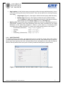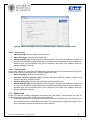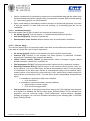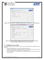
Download DICOM V6.3 USER MANUAL March 26th, 2015

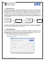
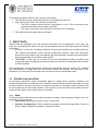
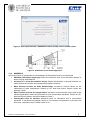
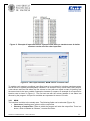
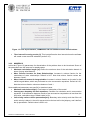
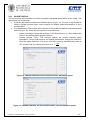
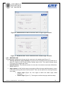
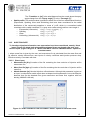
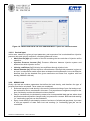
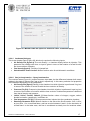
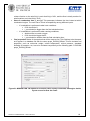
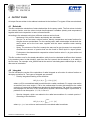
DICOM V6.3
USER MANUAL
March 26th, 2015
José M. García-Oliver, [email protected]
Walter Vera-Tudela, [email protected]
CMT – MOTORES TÉRMICOS  Camino de Vera s/nº  46022 Valencia. España  Tel. +34 963 877 650  Fax +34
963 877 659 E-mail: [email protected]  Web: http://www.cmt.upv.es
1
CONTENTS
INTRODUCTION ........................................................................................................... 3
2
USER INTERFACE ....................................................................................................... 3
3
INPUT DATA ................................................................................................................. 4
3.1
3.1.1
MAIN ................................................................................................................ 4
3.1.2
NUMERICS ...................................................................................................... 5
3.1.3
MORPHOLOGY ............................................................................................... 6
3.1.4
INJECTION RATE ............................................................................................ 7
3.1.5
MIXING LAW .................................................................................................... 8
3.2
4
5
STEADY CALCULATION ...................................................................... 4
TRANSIENT CALCULATION .............................................................. 10
3.2.1
MAIN .............................................................................................................. 11
3.2.2
NUMERICS .................................................................................................... 12
3.2.3
DISCRETIZATION ......................................................................................... 13
3.2.4
MORPHOLOGY ............................................................................................. 14
3.2.5
INJECTION RATE .......................................................................................... 15
3.2.6
MIXING LAW .................................................................................................. 16
OUTPUT FILES........................................................................................................... 19
4.1
Relst.dat .............................................................................................. 19
4.2
Integ.dat ............................................................................................... 19
4.3
temp1.dat ............................................................................................. 20
4.4
temp2.dat ............................................................................................. 20
4.5
xdata.dat .............................................................................................. 22
REFERENCES ............................................................................................................ 24
DICOM V6.3 USER MANUAL – March 26th 2015
2
1 INTRODUCTION
DICOM is a one-dimensional (1D) spray model that predicts the evolution of a turbulent jet under
some simplifying hypotheses. Scientific basis for the model can be found in [1-3]. This document
summarizes the main steps for a user to perform a calculation. The general flow of information is
described in Figure 1. The user interface is the only graphic interface of the program. It allows the
introduction of both the model needed input data, and also the location of the output data. This user
interface makes it possible to edit/manage/save an input file, which stores the configuration for one
case and launches the solver, which performs the calculations. After the calculation, output
information is written into text files, which can be later processed and analyzed with additional (not
provided) software.
USER
INTERFACE
CASE FILE
DICOM
SOLVER
OUTPUT
FILES
Figure 1. General flow of information in DICOM
In Section 2, a brief description is given of the general User Interface. In Section 3, the parameters
needed to create a calculation case will be explained, as well as how to feed them into the program.
Finally, Section 4 contains the description of output files.
2 USER INTERFACE
The user interface allows the introduction of input data, the management of input files and the
execution of the solver. A series of tabs have been arranged in the program main window to provide
the program with the necessary info to set up a case. On the other hand, there are three buttons on
the right-hand side of the user interface to manage input data files (Figure 2):
 Open: loads input data of a previous test from a text file.
 Save: saves the current case configuration case in a text file.
 Start: starts the calculation.
Figure 2. User input interface, ‘MAIN’ tab for Steady case.
DICOM V6.3 USER MANUAL – March 26th 2015
3
The working procedure with the user interface is as follows
 The user fills the input information directly or by uploading a case file.
 After clicking upon ‘Start’ The following events occur:
o The user is asked to save the input configuration in a file. This is a security just in
case this information has not been saved yet.
o The solver is launched, and calculation proceeds until it is finished.
 The code output information can be analyzed.
3 INPUT DATA
Different tabs are available in the user interface that allow for the configuration of one case. The
main one is the MAIN tab, where one can choose between the two main approaches for DICOM
calculation:
 STEADY: In this case, boundary conditions for spray development are constant with time.
This means time-constant nozzle injection parameters (injection mass and momentum
fluxes) and time-constant, fuel and ambient gas thermodynamic variables and composition.
All input parameters are therefore scalar values.
 TRANSIENT: In this case, all or some of the above-mentioned boundary conditions may
change with time. Accordingly, input data is made up of text files containing the time evolution
of these variables.
Even though there are few differences between both approaches, namely if some of the variables
are time-constant or change with time, the present section will describe the input form in two
subsections, the first one for the steady case, the second one for the transient case.
3.1 STEADY CALCULATION
As previously described, steady calculations apply for sprays where injection conditions and
chamber properties are constant with time. Therefore, there will not be need for input data in text file
format for injection, density or pressure in function of the time. All necessary input information will
be fed directly from the input user interface. The execution of the code will be much faster than the
transient case, where time evolution has to be tracked.
3.1.1 MAIN
The first tab allows selecting if the model is transient or steady. When selecting ‘Steady’ case, the
two fields on this screen are:
 Case name: Heading name given to all the output files.
 Directory of output files: Folder in which the program will write the output files. There is a
button, which is labeled as “Browse”, to select the folder.
DICOM V6.3 USER MANUAL – March 26th 2015
4
Figure 3. User input interface, 'NUMERICS' tab for steady cases. Default values.
Figure 4. Schematic of the model approach.
3.1.2 NUMERICS
In this tab (Figure 4), parameters for discretization of the problem have to be introduced:
 Maximum calculation length [m]: Define the maximum size of the calculation domain in
terms of spray axial distance.
 Increase in ‘x’ of the discretization dx [m]: Spatial discretization in the axial direction x,
which defines the cell size and corresponding spatial resolution.
 Mass Fraction increase for State Relationships: Increase in mixture fraction for the
calculations of state relationships. Default is 0.01. Note that mixture fraction values are
between 0 and 1.
 Mass Fraction increase for integral tables: Increase in mixture fraction on the axis for the
radial integral tables, which are performed to solve conservation equations. Default is 0.01.
Note that mixture fraction values are between 0 and 1.
 Convergence limit for iteration: Numerical value for calculation end in conservation
equations. If the difference between results of 2 successive computations is less than this
limit value, calculation stops. Default value is 10-6.
DICOM V6.3 USER MANUAL – March 26th 2015
5
Figure 5. User input interface, ‘MORPHOLOGY' tab for steady cases, single angle selection.
Figure 6. User input interface, ‘MORPHOLOGY' tab for steady cases, double angle selection.
3.1.3 MORPHOLOGY
In the next tab (Figure 5) there are some parameters that define the spray morphology, namely
geometry, speed profile and distribution of mass fraction.
 Velocity fraction for spray boundary: Numerical value that defines the spray radial limit in
terms of a fraction of the on-axis velocity. Default value is 0.01. This value is directly linked
to the spray cone angle input value.
 Schmidt number: The Schmidt number is in the ratio of momentum and mass diffusivities.
Default value is 1.
DICOM V6.3 USER MANUAL – March 26th 2015
6


Angle options: In this field the spray cone angle to define the spray radial boundary in terms
of the axial velocity profile has to be introduced. There are two options for selecting the spray
cone angle:
 Single angle (Figure 5): One angle to define the whole spray radial boundary.
 Double angle (Figure 6): Two angles to define the spray radial boundary.
The “Transition ‘x’ [m]” is the axial distance from the nozzle where the spray
angle change from the “Spray angle [º]” to the “Far-angle [º]”.
Radial profile: This section makes it possible to select one of the four mathematical functions
(Exponential, Spalding, Hinze and Schlichting) that have been considered for the radial
distribution of the conserved properties in terms of =r/R, which is a normalized radial
coordinate with r=radial coordinate, R = spray outer radius as derived from cone angle 𝜃.
o Exponential (=Gaussian)
𝑃𝑁(𝜉) = 𝑒𝑥𝑝(−𝐿𝑜𝑔(100) · 𝜉 2 )
o Spalding
𝑃𝑁(𝜉) = (1 + 𝑘𝜉 2 )−1
o Hinze
𝑃𝑁(𝜉) = (1 + 𝑘𝜉 2 )−2
o Schlichting (=Abramovich) 𝑃𝑁(𝜉) = (1 − 𝑘𝜉1.5 )2
3.1.4 INJECTION RATE
To introduce injection information, two approaches can be considered, namely ‘direct input’ (Figure
7) where both momentum and mass fluxes are given by the user, and ‘derived input’ (Figure 8),
where mass flow is given by the user, and momentum flux is calculated from the mass flow and an
effective velocity derived from user inputs of velocity coefficient and injection pressure drop.
Figure 7. 'INJECTION RATE' tab and ‘DIRECT INPUT’ option for steady cases.
DICOM V6.3 USER MANUAL – March 26th 2015
7
Figure 8. 'INJECTION RATE' tab and ‘DERIVED INPUT’ option for steady cases.
3.1.4.1 Direct input
 Momentum [N]: Injection orifice momentum flux.
 Mass flow [kg/s]: Injection orifice mass flux.
 Nozzle diameter [m]: Nominal injection orifice diameter. Although this parameter is given as
an input, in real practice model output does not depend on this parameter, but on the effective
diameter that can be obtained from given momentum and mass flow, together with fuel
density (MIXING LAW tab).
3.1.4.2 Derived input
In this case, mass flux is given as input parameter, and momentum flux is calculated from injection
pressure drop and velocity coefficient, considering Bernouilli Law.
 Mass flow [kg/s]: Injection orifice mass flux.
 Injection Pressure increase [Pa]: Pressure difference between injection system and
ambient into which injection occurs.
 Velocity Ratio Cv[-]: Velocity loss coefficient through injection hole.
 Nozzle diameter [m]: Nominal injection orifice diameter. Although this parameter is given as
an input, in real practice model output does not depend on this parameter, but on the effective
diameter that can be obtained from given momentum and mass flow, together with fuel
density (MIXING LAW tab).
3.1.5 MIXING LAW
Finally, the last tab contains parameters that define the local density, and therefore the type of
jet/spray flow that is calculated. Three cases are considered:
 Isothermal spray/jet: Local density is the result of isothermal mixing of pure fuel and pure air.
No combustion can be considered in this case. Fuel properties are neglected, except for the
pure fuel density and the stoichiometric mixture fraction.
DICOM V6.3 USER MANUAL – March 26th 2015
8


Gas jet: Local density is calculated by means of an incompressible ideal gas law, where local
temperature and composition change locally, but pressure is constant. Both inert and reacting
(i.e. combusting) gas jets can be considered.
Spray: Local density is calculated by means of a mixture of a liquid and gas phase, by means
of real gas equation of state. Both inert and reacting (i.e. combusting) gas jets can be
considered.
3.1.5.1 Isothermal jet/spray
This is the simplest case (Figure 9) which only requires the following inputs:
 Air density [kg/m3]: Pure air density, i.e. chamber density before de injection.
 Fuel density [kg/m3]: Density of injected fuel.
 Stoichiometric mass fraction: Mixture fraction value for stoichiometric conditions.
3.1.5.2 Gas jet– Spray
The next two cases (Figure 10) require the same input data, and the difference between both cases
is the state of injected fuel, gas or liquid, respectively.






Air density [kg/m3]: Density in the chamber into which injection is performed.
Pressure [Pa]: Pressure in the chamber into which injection is performed. Chamber
temperature is calculated from pressure and density.
Yn2inf, Yo2inf, Yco2inf, Yh2oinf [-]: Mass fraction values of nitrogen, oxygen, carbon
dioxide and water, respectively, in ambient air.
Fuel temperature Tfo [K]: Fuel temperature when injected into the combustion chamber.
Reactivity Parameter fLOL[-]: Mixture fraction on the axis at the lift-off location. fLOL is 0
for an inert flow, 1 for a non-lifted flame, and has a value between 0 and 1 for the simulation
of a lifted flame. In the latter case, the flow is considered as totally inert for locations where
mixture fraction on the axis fcl(x) is such that fcl(x)> fLOL, and the flow is totally reactive for
axial locations such that fcl(x)< fLOL. The user has to check incompatibility among different
inputs:
o If a calculation is performed under inert conditions:
 fLOL should be 0
o If a calculation is performed under reacting conditions,
 Ambient has to contain oxygen
 fLOL should be bigger than 0
Fuel properties: Name of the species that will be used as fuel. This field has to be the same
as it appear in a database file with the name props_DICOM_DB.dat. This file includes fuel
properties, such as molecular weight, critical temperature, critical pressure, standard
enthalpy of formation, etc, has to be included compulsorily at the following path: C:\DICOM\
props_DICOM_DB.dat.
DICOM V6.3 USER MANUAL – March 26th 2015
9
Figure 9. User input interface, ’MIXING LAW' tab option for steady cases. Isothermal spray.
Figure 10. User input interface, ’MIXING LAW' tab option for steady cases. Gas jet is
selected, although a similar layout occurs for Spray cases.
3.2 TRANSIENT CALCULATION
The transient approach makes it possible to introduce a time-variable boundary condition out of the
following:
 Injection mass/momentum flux, to model variable injection cases.
 In-cylinder thermodynamic conditions (pressure and density, which also may entail a time
evolution of temperature) to simulate engine changing conditions.
 Flow chemical state, i.e. a transition from inert to reacting conditions at a defined time instant
(mixture ignition).
DICOM V6.3 USER MANUAL – March 26th 2015
10
Figure 11. Example of input text files for injection mass flux in a transient case. A similar
structure can be used for other input files.
Figure 12. User input interface, 'MAIN' tab for Transient case.
To enable such transient conditions input files have to be provided for injection mass/momentum
flux as well as in-cylinder thermodynamic variables. The structure of any of such files is fairly simple,
a two-column ascii text file where the first column is time (with zero equal to start of injection) and
the second one is the input variable. Separation character is a space. An example of an input file for
injection rate is shown in Figure 11. The first text row with the column headers is not taken into
account by the program. All input file variables are expressed in terms of SI units.
3.2.1 MAIN
The interface is similar to the steady case. The following fields can be selected (Figure 12):
 Case name: Heading name given to all the output files.
 Directory of output files: Folder in which the program will write the output files. There is a
button, which is labeled as “Browse”, to select the folder.
DICOM V6.3 USER MANUAL – March 26th 2015
11
Figure 13. User input interface, 'NUMERICS' tab for transient cases. Default values.

Time interval for saving results [s]: This input defines the time interval where the software
will create a new result file xdata.dat (section 4.5).
3.2.2 NUMERICS
In this tab (Figure 13) parameters for discretization of the problem have to be introduced. Some of
the parameters are the same as for steady cases:
 Maximum calculation length [m]: Define the maximum size of the calculation domain in
terms of spray axial distance.
 Mass Fraction increase for State Relationships: Increase in mixture fraction for the
calculations of state relationships. Default is 0.01. Note that mixture fraction values are
between 0 and 1.
 Mass fraction increase for integral tables: Increase in mixture fraction on the axis for the
radial integral tables, which are performed to solve conservation equations. Default is 0.01.
Note that mixture fraction values are between 0 and 1.
Some additional parameters are specific for transient cases:
 Maximum calculation time[s]: Final instant of calculation of the model.
 Convergence boundary for main equations: Condition for calculation end in conservation
equations. If the difference between results of two successive computations is less than this
limit value, calculation stops. Default value is 10-8.
 Cell velocity value to define penetration[m/s]: Boundary value velocity such that if the cell
outlet velocity is below it, the cell is assumed to be the last cell in the jet/spray, and it defines
the tip penetration. Default value is 0.001 m/s.
DICOM V6.3 USER MANUAL – March 26th 2015
12
3.2.3 DISCRETIZATION
This tab contains the information for both the temporal and spatial discretization of the model. Two
approaches can be selected:
 Automatic discretization makes use of default values (Figure 14). The user is only allowed to
modify a ‘Spatial increase factor, which modifies the default spatial discretization x by a
constant factor.
 Free discretization: This method allows the user to fully modify the details of the discretization
method (Figure 15), which are summarized in two parameters:
o Spatial increase[m]: Spatial discretization in the axial direction x, which defines the
cell size and corresponding spatial resolution.
o Courant Number (CFL): This constant defines the relation between spray
propagation, velocity and temporal and spatial discretization through the definition.
Once the spatial resolution x is given, time step t can be calculated by means of
CFL and the local flow velocity by means of ∆𝑡 =
𝐶𝐹𝐿∆𝑥
𝑢
Figure 14. 'DISCRETIZATION' tab for transient cases. Automatic option.
Figure 15. 'DISCRETIZATION' tab for transient cases. Free discretization option.
DICOM V6.3 USER MANUAL – March 26th 2015
13
Figure 16. ‘MORPHOLOGY' tab for transient cases, single angle selection.
Figure 17. ‘MORPHOLOGY' tab for transient cases, double angle selection.
3.2.4 MORPHOLOGY
The parameters introduced in this part are the same as in the steady case (Figure 17).
 Velocity fraction for spray boundary: Numerical value that defines the spray radial limit in
terms of a fraction of the on-axis velocity. Default value is 0.01. This value is directly linked
to the spray cone angle input value.
 Schmidt number: The Schmidt number is in the ratio of momentum and mass diffusivities.
Default value is 1.
 Angle options: In this field the spray cone angle to define the spray radial boundary in terms
of the axial velocity profile has to be introduced. There are two options for selecting the spray
cone angle:
 Single angle (Figure 16): One angle to define the whole spray radial
boundary.
 Double angle (Figure 17): Two angles to define the spray radial boundary.
DICOM V6.3 USER MANUAL – March 26th 2015
14

3.2.5
The “Transition ‘x’ [m]” is the axial distance from the nozzle where the spray
angle change from the “Spray angle [º]” to the “Far-angle [º]”.
Radial profile: This section makes it possible to select one of the four mathematical functions
(Exponential, Spalding, Hinze and Schlichting) that have been considered for the radial
distribution of the conserved properties in terms of =r/R, which is a normalized radial
coordinate with r=radial coordinate, R = spray outer radius as derived from cone angle 𝜃.
o Exponential (=Gaussian)
𝑃𝑁(𝜉) = 𝑒𝑥𝑝(−𝐿𝑜𝑔(100) · 𝜉 2 )
o Spalding
𝑃𝑁(𝜉) = (1 + 𝑘𝜉 2 )−1
o Hinze
𝑃𝑁(𝜉) = (1 + 𝑘𝜉 2 )−2
o Schlichting (=Abramovich) 𝑃𝑁(𝜉) = (1 − 𝑘𝜉1.5 )2
INJECTION RATE
To introduce injection information, two approaches have been considered, namely ‘direct
input’ (Figure 18) where both momentum and mass fluxes are given by the user; and
‘derived input’ (Figure 19Figure 19. 'INJECTION RATE' tab and ‘DERIVED INPUT’ option for
transient cases.
), where mass flow is given by the user, and momentum flux is calculated from the mass flow and
an effective velocity derived from user inputs of velocity coefficient and injection pressure drop.
Effective velocity is constant with time.
3.2.5.1 Direct input
 Momentum file [N-s]: Location of the file containing the time evolution of injection orifice
momentum flux.
 Mass flow file [kg/s-s]: Location of the file containing the time evolution of injection orifice
mass flux.
 Nozzle diameter [m]: Nominal injection orifice diameter. Although this parameter is given as
an input, in real practice model output does not depend on this parameter, but on the effective
diameter that can be obtained from given momentum and mass flow, together with fuel
density (MIXING LAW tab).
Figure 18. 'INJECTION RATE' tab and ‘DIRECT INPUT’ option for transient cases.
DICOM V6.3 USER MANUAL – March 26th 2015
15
Figure 19. 'INJECTION RATE' tab and ‘DERIVED INPUT’ option for transient cases.
3.2.5.2 Derived input
In this case, mass flux is given as input parameter, and momentum flux is calculated from injection
pressure drop and velocity coefficient, considering Bernouilli’s Law.
 Mass flow file [kg/s-s]: Location of the file containing the time evolution of injection orifice
mass flux.
 Injection Pressure increase [Pa]: Pressure difference between injection system and
ambient into which injection occurs.
 Velocity coefficient Cv[-]: Velocity loss coefficient through injection hole.
 Nozzle diameter [m]: Nominal injection orifice diameter. Although this parameter is given as
an input, in real practice model output does not depend on this parameter, but on the effective
diameter that can be obtained from given momentum and mass flow, together with fuel
density (MIXING LAW tab).
3.2.6 MIXING LAW
Finally, the last tab contains parameters that define the local density, and therefore the type of
jet/spray flow that is calculated. Three cases are considered:
 Isothermal spray/jet: Local density is the result of isothermal mixing of pure fuel and pure air.
No combustion can be considered in this case. Fuel properties are neglected, except for the
pure fuel density and the stoichiometric mixture fraction.
 Gas jet: Local density is calculated by means of an incompressible ideal gas law, where local
temperature and composition change locally, but pressure is constant. Both inert and reacting
(i.e. combusting) gas jets can be considered.
 Spray: Local density is calculated by means of a mixture of a liquid and gas phase, by means
of real gas equation of state. Both inert and reacting (i.e. combusting) gas jets can be
considered.
DICOM V6.3 USER MANUAL – March 26th 2015
16
Figure 20. ’MIXING LAW' tab option for transient cases. Isothermal spray.
3.2.6.1 Isothermal jet/spray
This is the simplest case (Figure 20) which only requires the following inputs:
 Air Density File [kg/m3-s]: Pure air density, i.e. chamber density before de injection. This
parameter can change with time, so input is given in terms of the location of a text file with
the time evolution of density.
 Fuel density [kg/m3]: Density of injected fuel.
 Stoichiometric mass fraction: Mixture fraction value for stoichiometric conditions.
3.2.6.2 Gas jet inert/reactive – Spray inert/reactive
The next two cases (Figure 21) require the same input data, but the difference between both cases
resides in the state of injected fuel, gas or liquid, respectively. In this case, particular fuel properties
are considered depending on the compilation.
 Air Density File [kg/m3]: Density in the chamber into which injection is performed. It’s given
in terms of the location of a text file with the time evolution of density.
 Pressure File [Pa]: Pressure in the chamber into which injection is performed. Input is given
in terms of the location of a text file with the time evolution. Ambient temperature is obtained
from that of density and pressure.
 Yn2inf, Yo2inf, Yco2inf, Yh2oinf [-]: Mass fraction values of nitrogen, oxygen, carbon
dioxide and water, respectively, in ambient air.
 Fuel temperature Tfo [K]: Fuel temperature when injected into the combustion chamber.
 Reactivity Parameter fLOL: Mixture fraction on the axis at the lift-off location. fLOL is 0 for
an inert flow, 1 for a non-lifted flame, and has a value between 0 and 1 for the simulation of
a lifted flame. In the latter case, the flow is considered as totally inert for locations where
DICOM V6.3 USER MANUAL – March 26th 2015
17


mixture fraction on the axis fcl(x) is such that fcl(x)> fLOL, and the flow is totally reactive for
axial locations such that fcl(x)< fLOL.
Start of combustion time, t_soc [s]: This parameter indicates the time instant at which
combustion begins. The user has to check incompatibility among different inputs:
o If a calculation is performed under inert conditions:
 fLOL should be 0
 t_soc should be bigger than the final calculation time.
o If a calculation is performed under reacting conditions,
 Ambient has to contain oxygen
 fLOL should be bigger than 0
 t_soc should be smaller than the final calculation time.
Fuel properties: Name of the species that will be used as fuel. This field has to be the same
as it appear in a database file with the name props_DICOM_DB.dat. This file includes fuel
properties, such as molecular weight, critical temperature, critical pressure, standard
enthalpy of formation, etc, has to be included compulsorily at the following path: C:\DICOM\
props_DICOM_DB.dat.
Figure 21.’MIXING LAW' tab option for transient cases. Spray is selected, although a similar
layout occurs for Gas Jet cases.
DICOM V6.3 USER MANUAL – March 26th 2015
18
4 OUTPUT FILES
All output files are written in the address introduced in the interface. Five types of files are calculated:
4.1 Relst.dat
This file contains the calculation of state relationships for the spray model. The first column includes
the mixture fraction, and the others include thermodynamic variables (density and temperature)
together with local composition in terms of mass fraction.
According to the selected mixing law, different versions can be found:
- Isothermal: Only mixture fraction and density are calculated.
- Gas jet: For an inert case, mixture fraction, density, temperature and mass fractions for
the gas mixture are tabulated. For the reacting case, state relationships include both the
same values as for the inert case, together with the same variables under reacting
conditions.
- Spray: The structure of the file is exactly the same as for gas jet cases, but composition
considers the amount of species that can be found in either liquid or vapour phase.
Furthermore, the characteristic evaporation mixture fraction value fevap is given at the end
of the first row.
This file is written once for the steady calculation, while it can be calculated at different time instants
in the transient case. In that situation, each time the file is saved, the timestamp in s is added to
the file name. For example: relst_000100.dat is the result of calculating state relationships at 100s
after start of calculation.
4.2 Integ.dat
This file includes the results of the calculation of radial integrals as a function of mixture fraction on
the spray centerline fcl. Two types of integrals are recorded:
- Density integrals according to the definition:
𝐼𝑁𝑇(𝑓𝑐𝑙 , 𝐺, 𝜃) = ∫  · 𝑃𝑁 𝐺 (𝜉)𝜉𝑑𝜉
where =r/R is a normalized radial coordinate with r=radial coordinate, R = spray outer radius
as derived from cone angle 𝜃. PN is the mathematical function that describes the radial
evolution of conservative variables as described in the Morphology Tab, and G is a parameter
that depends on the term of the conservation equation where the integral is performed, in
particular G can be equal to 1, 2, Sc, 1+Sc or 0.
-
Species integrals, which are related to the radial accumulation of a certain species ‘i’
according to the definition:
𝜉𝑚𝑎𝑥
𝐼𝑁𝑇(𝑓𝑐𝑙 , 𝐺, 𝜃) = ∫
𝜉𝑚𝑖𝑛
 · 𝑌𝑖 · 𝜉𝑑𝜉
where min, min, is a minimum and maximum normalized radial coordinate.
DICOM V6.3 USER MANUAL – March 26th 2015
19
Density integrals are always recorded, while species integrals depend on the mixing law. This file is
written once for the steady calculation, while it can be calculated at different time instants in the
transient case. In that situation, each time the file is saved, the timestamp in s is added to the file
name. For example: integ_000100.dat is the result of radial integrals at 100s after start of
calculation. The file is always calculated whenever news state relationships are calculated.
4.3 temp1.dat
DICOM calculates with a small time step depending on previously discussed discretization
considerations. File temp1.dat records the time evolution of boundary conditions for the spray
problem.
The first column for this file is time, and the rest of the columns include the following variables:
VARIABLE
u0
UNITS
m/s
DEFINITION
Effective injection velocity at the nozzle exit.
I0
N
Injection momentum flux at the nozzle exit.
M0
kg/s
Injection mass flux at the nozzle exit.
rho_a
kg/m3
Ambient air density inside the chamber where the spray is injected..
rho_f
do
kg/m3
m
fst
Ta
Tst
fLOL
fevap
K
K
-
Injected fuel density.
Effective nozzle diameter, as calculated from momentum, mass flux and
injected fuel density.
Mixture fraction of stoichiometric conditions.
Air temperature.
Temperature of stoichiometric surface.
Mixture fraction at the lift-off location.
Fully evaporation mixture fraction (only for liquid spray cases).
One row is written per calculation time step in transient cases. For steady ones, boundary conditions
do not change, and the file has only one row, where time column is omitted.
4.4 temp2.dat
This file records the time evolution of the main results from the model in terms of global parameters.
The format of the file is exactly the same for both the steady and the transient model formulations.
The file has exactly the same structure as temp1.dat, i.e. a time column followed by a number of
columns with different variables, depending on the mixing law case and according to the following
list:
VARIABLE
S
S_
UNITS
m
m
DEFINITION
Maximum jet tip penetration.
Maximum penetration of a surface with a characteristic equivalence ratio
.
DICOM V6.3 USER MANUAL – March 26th 2015
20
S_evap,
S_evap_o
m
miny
kg
Maximum liquid length as calculated from the spray tip towards the nozzle
(S_evap) or from the nozzle to the tip of the spray (S_evap_o). Only one
of them is provided in steady cases
Integral of the mixture fraction all over the spray. It should be equal to the
injected fuel mass until the corresponding time.
𝑠𝑅
𝑚𝑖𝑛𝑦 = ∬  ∙ 𝑓 ∙ 2𝜋𝑟 ∙ 𝑑𝑟 ∙ 𝑑𝑥
00
mfmix_
kg
Integral of fuel mass below a characteristic equivalence ratio .
𝑠𝑅
𝑚𝑓,𝑚𝑖𝑥 = ∬  ∙ 𝑓 ∙ 2𝜋𝑟 ∙ 𝑑𝑟 ∙ 𝑑𝑥
0 𝑅
mf_mixevap
kg
Integral of fuel mass outside of the iso-surface of evaporation mixture
fraction fevap.
𝑠𝑅
∬  ∙ 𝑓 ∙ 2𝜋𝑟 ∙ 𝑑𝑟 ∙ 𝑑𝑥
𝑚𝑓,𝑚𝑖𝑥𝑒𝑣𝑎𝑝 =
0 𝑅𝑒𝑣𝑎𝑝
ma
kg
Integral of the mixture fraction all over the spray.
𝑠𝑅
𝑚𝑎 = ∬  ∙ (1 − 𝑓) ∙ 2𝜋𝑟 ∙ 𝑑𝑟 ∙ 𝑑𝑥
00
LOL
mfsq
m
kg
Lift-Off Length based upon input fLOL (fLOL=0 for inert spray).
Integral of the fuel mass all over the spray. It should be equal to the
injected fuel mass for inert cases. For reacting ones, it corresponds to the
unburned fuel mass.
𝑠𝑅
𝑚𝑓,𝑠𝑞 = ∬  ∙ 𝑌𝑓 ∙ 2𝜋𝑟 ∙ 𝑑𝑟 ∙ 𝑑𝑥
00
mf_q
kg
mO2,
mCO2,
mH2O
kg
mfl,
mfv
kg
Integral of the burned fuel mass all over the spray.
𝑚𝑓,𝑞 = 𝑚𝑖𝑛𝑦 − 𝑚𝑓,𝑠𝑞
Integral of a characteristic species (O2, CO2, H2O) all over the spray.
𝑠𝑅
𝑚𝑖 = ∬  ∙ 𝑌𝑖 ∙ 2𝜋𝑟 ∙ 𝑑𝑟 ∙ 𝑑𝑥
00
Integral of the fuel mass all over the liquid (l) or vapour (v) part of the
spray, respectively.
𝑠𝑅
𝑚𝑓,𝑙 = ∬  ∙ 𝑌𝑓,𝑙 ∙ 2𝜋𝑟 ∙ 𝑑𝑟 ∙ 𝑑𝑥
00
𝑠𝑅
𝑚𝑓,𝑣 = ∬  ∙ 𝑌𝑓,𝑣 ∙ 2𝜋𝑟 ∙ 𝑑𝑟 ∙ 𝑑𝑥
00
uclmax
m/s
x_uclmax
fclmax
m
-
x_fclmax
m
Maximal velocity along the axis at every time step (only for transient
cases).
Axial location where uclmax is found (only for transient cases).
Maximal mixture fraction along the axis at every time step (only for
transient cases).
Axial location where fclmax is found (only for transient cases).
DICOM V6.3 USER MANUAL – March 26th 2015
21
4.5 xdata.dat
This file includes, for a certain time instant, the evolution along the spray axis of the following
variables:
VARIABLE
xeje
UNITS
m
ucl
fcl
I
m/s
N
DEFINITION
Axial coordinate. For transient cases, this variable ranges
from zero to the spray tip penetration at the corresponding
time step. For steady cases, this variables ranges from
zero to the user-defined “Domain x-size” in the Numerics
Tab.
Axial component of the velocity vector on the centerline.
Mixture fraction on the centerline.
Radially integrated momentum flux (only for transient
cases).
𝑅
𝐼 = ∫  ∙ 𝑢2 ∙ 2𝜋𝑟 ∙ 𝑑𝑟
0
Mf
kg/s
Radially integrated fuel mass flux (only for transient cases).
𝑅
𝑀𝑓 = ∫  ∙ 𝑢 ∙ 𝑌𝑓 ∙ 2𝜋𝑟 ∙ 𝑑𝑟
0
M
kg/s
Radially integrated total mass flux.
𝑅
𝑀 = ∫  ∙ 𝑢 ∙ 2𝜋𝑟 ∙ 𝑑𝑟
0
umed
m/s
fmed
-
rho_cl
rho_med
rho_med_flow
kg/m3
kg/m3
R
Rini_u
Rini_f
R_
Revap
m
m
m
m
Cross-sectional average velocity from the ratio of
momentum and mass fluxes.
𝐼
𝑢𝑚𝑒𝑑 =
𝑀
Cross-sectional average velocity from the ratio of fuel and
total mass fluxes.
𝑀𝑓
𝑓𝑚𝑒𝑑 =
𝑀
Density on the centerline.
Cross-sectional average density from the average mixture
fraction (rho_med) or from the ratio of mass and volume
fluxes (rho_med_flow).
Spray radius.
Radius of the intact zone in terms of axial velocity (Rini_u)
or mixture fraction (Rini_f)
Radius where a certain equivalence ratio  is found.
Radius where a mixture fraction for full evaporation fevap
is found (only for liquid spray calculations).
DICOM V6.3 USER MANUAL – March 26th 2015
22
mf
kg/m
Radial integral of total fuel mass, i.e. total fuel mass per
unit length.
𝑅
𝑚𝑓 = ∫  ∙ 𝑓 ∙ 2𝜋𝑟 ∙ 𝑑𝑟
0
mfmix_
kg/m
Radial integral of fuel mass from R_ to R, i.e. total fuel
mass per unit length below a characteristic equivalence
ratio .
𝑅
𝑚𝑓𝑚𝑖𝑥 = ∫  ∙ 𝑓 ∙ 2𝜋𝑟 ∙ 𝑑𝑟
𝑅
mfmixevap
kg/m
Radial integral of fuel mass from R_evap to R, i.e. total fuel
mass per unit length outside of fevap iso-surface.
𝑅
∫  ∙ 𝑓 ∙ 2𝜋𝑟 ∙ 𝑑𝑟
𝑚𝑓𝑚𝑖𝑥𝑒𝑣𝑎𝑝 =
𝑅𝑒𝑣𝑎𝑝
ma
kg/m
Radial integral of total air mass, i.e. total air mass per unit
length.
𝑅
𝑚𝑎 = ∫  ∙ (1 − 𝑓) ∙ 2𝜋𝑟 ∙ 𝑑𝑟
0
mf_sq
kg/m
Radial integral of unburned fuel mass, i.e. unburned fuel
mass per unit length.
𝑅
𝑚𝑓𝑠𝑞 = ∫  ∙ 𝑌𝑓 ∙ 2𝜋𝑟 ∙ 𝑑𝑟
0
mfl,
mfv
kg/m
Radial integral of fuel mass in liquid mfl or vapour mfv
phase.
𝑅
𝑚𝑓𝑙 = ∫  ∙ 𝑌𝑓,𝑙 ∙ 2𝜋𝑟 ∙ 𝑑𝑟
0
𝑅
𝑚𝑓𝑣 = ∫  ∙ 𝑌𝑓,𝑣 ∙ 2𝜋𝑟 ∙ 𝑑𝑟
0
mO2,
mCO2,
mH2O
kg/m
Tcl
Tmed
K
K
Yi_cl
-
Radial integral of a certain species i (e.g. O2, CO2, H2O)
𝑅
𝑚𝑖 = ∫  ∙ 𝑌𝑖 ∙ 2𝜋𝑟 ∙ 𝑑𝑟
0
Temperature on the centerline.
Cross-sectional average temperature from the average
mixture fraction
Mass fraction of species i on the centerline.
For transient cases, the program creates one file after a characteristic time has elapsed. This time
interval is selected by the user in the MAIN tab. The filename includes the timestamp in s. For
steady cases, only one file is recorded with the same information and no time stamp.
DICOM V6.3 USER MANUAL – March 26th 2015
23
5 REFERENCES
[1] Pastor J.V., López J.J., Garcia-Oliver J.M., Pastor J.M., “A 1D model for the description of mixingcontrolled inert diesel sprays”, Fuel 87 (2008) 2871-2885
[2] Desantes J.M., Pastor J.V., Garcia-Oliver J.M., Pastor J.M., “A 1D model for the description of
mixing-controlled reacting diesel sprays”, Combustion and Flame 156 (2009) 234–249
[3] Pastor, J., Payri, R., Garcia-Oliver, J., and Nerva, J., "Schlieren Measurements of the ECN-Spray
A Penetration under Inert and Reacting Conditions," SAE Technical Paper 2012-01-0456, 2012
[4] Pastor, J., Garcia-Oliver, J., Pastor, J.M. and Vera-Tudela, W., “One- Dimensional Diesel Spray
Modeling of Multicomponent Fuels”, Atomization and Sprays, in press, 2015, DOI
10.1615/AtomizSpr.2014010370
DICOM V6.3 USER MANUAL – March 26th 2015
24