Download GGU-CONSOLIDATE - Index of

Analysis of one-dimensional consolidation processes
in single- and multi-layered systems
GGU-CONSOLIDATE
VERSION 5
Last revision:
April 2012
Prof. Dr. Johann Buß
Copyright:
Technical implementation and sales: Civilserve GmbH, Steinfeld
Contents:
1 Preface .................................................................................................................................. 5
2 Licence protection and installation .................................................................................... 7
3 Language selection............................................................................................................... 7
4 Starting the program ........................................................................................................... 8
5 Theoretical principles .......................................................................................................... 9
5.1 Consolidation theory after Terzaghi and analytical solution............................................ 9
5.2 Numerical solution with difference equations................................................................ 11
5.2.1 Fundamentals ......................................................................................................... 11
5.2.2 Multi-layered system ............................................................................................. 11
5.2.3 Continuous load application .................................................................................. 12
5.3 Consolidation settlements for non-linear compression .................................................. 13
5.4 Analytical solution with vertical drainage...................................................................... 15
5.5 Numerical solution with vertical drainage ..................................................................... 16
5.6 Secondary settlements .................................................................................................... 16
6 Short introduction using worked examples..................................................................... 20
6.1 Example system.............................................................................................................. 20
6.2 Test 1: Consolidation (analytical) .................................................................................. 21
6.3 Test 2: Consolidation (numerical).................................................................................. 24
6.4 Test 3: Consolidation (numerical) with real pore water pressure distribution ............... 26
6.5 Test 4: Consolidation (numerical) with real pore water pressure distribution and
time-dependent loading function.................................................................................... 28
6.6 Test 5: Consolidation (numerical) with real pore water pressure distribution and
time-dependent loading function and boundary condition............................................. 29
6.7 Test 6: Consolidation (analytical) with vertical drains................................................... 29
6.8 Test 7: Consolidation (numerical) with vertical drains and actual pore water
pressure distribution and time-dependent loading function ........................................... 31
6.9 Test 8: Worked example with compression index CC .................................................... 33
7 Description of menu items................................................................................................. 36
7.1 File menu........................................................................................................................ 36
7.1.1 "New" menu item................................................................................................... 36
7.1.2 "Load" menu item.................................................................................................. 36
7.1.3 "Save" menu item .................................................................................................. 36
7.1.4 "Save as" menu item .............................................................................................. 37
7.1.5 "Printer preferences" menu item............................................................................ 37
7.1.6 "Print and export" menu item ................................................................................ 37
7.1.7 "Batch print" menu item ........................................................................................ 39
7.1.8 "Exit" menu item.................................................................................................... 39
7.1.9 "1, 2, 3, 4" menu items........................................................................................... 39
7.2 Edit menu ....................................................................................................................... 40
7.2.1 "Project identification" menu item......................................................................... 40
7.2.2 "Type of consolidation" menu item ....................................................................... 40
7.2.3 "System parameters" menu item ............................................................................ 41
7.2.3.1 Analytical methods........................................................................................ 41
7.2.3.2 Numerical methods........................................................................................ 43
GGU-CONSOLIDATE User Manual
Page 2 of 71
April 2012
7.2.4 "Define times" menu item...................................................................................... 44
7.2.5 "Soils" menu item .................................................................................................. 45
7.2.6 "Soils (reloading)" menu item ............................................................................... 47
7.2.7 "Pore water pressure (max)" menu item ................................................................ 47
7.2.8 "Boundary conditions" menu item......................................................................... 48
7.2.9 "Load increase" menu item.................................................................................... 49
7.2.10 "Secondary settlements" ........................................................................................ 50
7.2.11 "Installation time (vertical drains)" menu item...................................................... 51
7.2.12 "cv(axial)/cv" menu item ....................................................................................... 51
7.3 System menu .................................................................................................................. 51
7.3.1 "Analyse" menu item ............................................................................................. 51
7.4 Output preferences menu ............................................................................................... 52
7.4.1 "General legend" menu item.................................................................................. 52
7.4.2 "Pore water pressure/consolidation ratio" menu item............................................ 53
7.4.3 "Time-settlement" menu item ................................................................................ 55
7.4.4 "System presentation" menu item .......................................................................... 56
7.4.5 "Output table" menu item ...................................................................................... 57
7.4.6 "Soil properties legend" menu item ....................................................................... 58
7.4.7 "Load curve" menu item ........................................................................................ 59
7.4.8 "Pore ratio diagram" menu item............................................................................. 60
7.4.9 "Page size and margins" menu item....................................................................... 61
7.4.10 "Move objects" menu item..................................................................................... 61
7.5 Graphics preferences menu ............................................................................................ 62
7.5.1 "Refresh and zoom" menu item ............................................................................. 62
7.5.2 "Zoom info" menu item ......................................................................................... 62
7.5.3 "Legend font selection" menu item........................................................................ 62
7.5.4 "With borders" menu item ..................................................................................... 62
7.5.5 "Pen colour and width" menu item ........................................................................ 63
7.5.6 "Mini-CAD toolbar" menu item ............................................................................ 63
7.5.7 "Toolbar preferences" menu item .......................................................................... 64
7.5.8 "Load graphics preferences" menu item ................................................................ 65
7.5.9 "Save graphics preferences" menu item................................................................. 65
7.6 ? menu ............................................................................................................................ 66
7.6.1 "Copyright" menu item .......................................................................................... 66
7.6.2 "Help" menu item .................................................................................................. 66
7.6.3 "GGU on the web" menu item ............................................................................... 66
7.6.4 "GGU support" menu item..................................................................................... 66
7.6.5 "What's new?" menu item...................................................................................... 66
7.6.6 "Language preferences" menu item ....................................................................... 66
8 Tips and tricks.................................................................................................................... 67
8.1 Keyboard and mouse...................................................................................................... 67
8.2 Function keys ................................................................................................................. 68
8.3 "Copy/print area" icon.................................................................................................... 68
9 Index.................................................................................................................................... 69
GGU-CONSOLIDATE User Manual
Page 3 of 71
April 2012
List of figures:
Figure 1 Consolidation layer .........................................................................................................10
Figure 2 Step function....................................................................................................................12
Figure 3 Stress - pore ratio relationship (GGU-OEDOM program).............................................13
Figure 4 Stress - compression index relationship (GGU-OEDOM program)...............................14
Figure 5 Vertical drains.................................................................................................................15
Figure 6 Example system ...............................................................................................................20
Figure 7 Section of example system ...............................................................................................33
Figure 8 Pore water pressure diagram test 8 ................................................................................35
GGU-CONSOLIDATE User Manual
Page 4 of 71
April 2012
1 Preface
If cohesive layers are loaded faster than they can expel their pore water, excess pore water pressures result, which are only gradually dissipated. This process is known as consolidation.
Settlement analyses to DIN 4019 do not take the fact into consideration that a large part of the
settlement is often already complete during the construction phase. Most buildings are already
being subjected to 80% of final loads by the time the shell is complete. Settlements, and therefore
differential settlements, are generally non-critical at this stage, as they are manifested in masonry
and other joints, which are then covered by pointing and paintwork in the "post-shell" phase. For
cohesive soils in particular, therefore, a forecast of the temporal development of settlements, even
for "simple" buildings, is an vital prerequisite for the safe judgement of possibly damaging differential settlements. The GGU-CONSOLIDATE program can assist you in these tasks.
The GGU-CONSOLIDATE program system allows the analysis of one-dimensional consolidation processes in single and multi-layered systems. Any pore water distribution configuration may
be defined. Using this program, you can also generate a pore water pressure distribution resulting
from a foundation load. The de-watering conditions at the upper and lower layer boundaries can
be defined separately. A load can also be applied to the system as a function of the time. It is also
possible to take secondary settlements into consideration.
Beside the calculation of analytically derived solutions (Terzaghi), the GGU-CONSOLIDATE
program is also capable of numerically modelling multi-layered systems. As well as classical consolidation theory, systems with installed vertical drainage can also be investigated. A combination
of both systems (with and without vertical drainage) is also possible.
Thus, five different consolidation types are offered:
 Consolidation (analytical)
One-dimensional consolidation theory after Terzaghi for a system with one layer and constant pore water pressure distribution across the whole layer depth at time t = 0. Modelling
is performed using the analytical relationships given in the literature.
 Consolidation (numerical)
One-dimensional consolidation theory after Terzaghi for a system with several layers and
arbitrary pore water pressure distribution at time t = 0. Furthermore, loading can be defined
as a function of time. Modelling is numerical, using difference equations. The modelling of
one-layer systems with constant pore water distribution using available analytical solutions
as described above can of course also be performed with the numerical model. Analytical
consolidation has nevertheless been incorporated into the program, as this solution will always require shorter calculation times. Furthermore, you can check the very good quality
of the numerical solution on simple examples.
 Consolidation (analytical) with vertical drainage
Consolidation theory in a system with vertical drains. Pore water pressure dissipation is always directed horizontally towards the vertical drains. The pore water pressure is therefore
temporally constant across the whole layer depth. Input of layer thickness in such systems
is superfluous and has no influence on the temporal course of settlement.
 Consolidation (numerical) with vertical drainage
In complete analogy to analytical modelling, a multi-layer system with vertical drainage
can be processed. Here too, pore water pressure dissipation is exclusively horizontal towards the vertical drains. The pore water pressure is therefore temporally constant in each
layer. As the pore water pressure is integrated across the layer for the whole time range,
layer thickness input for multiple layer systems is important for the temporal settlement
course, in contrast to one-layer systems.
GGU-CONSOLIDATE User Manual
Page 5 of 71
April 2012
 Consolidation (numerical) with both types
It is possible to investigate systems in which vertical drains are only installed at a later,
user-defined time.
All principal data and modelling results will be displayed on the screen. A total of five, or eight,
graphical elements (see menu "Output preferences") can be presented:
 Legend with general information
 Table with the consolidation values at specified times
 Pore water pressure profile/consolidation ratio across the layer depth
 System visualisation
 Time-dependent development of degree of consolidation, settlement or pore water pressure
 Legend with soil properties (numerical modelling only)
 Type of load increase (numerical modelling only)
 Pore ratio diagram (only for calculation with the compression index CC)
The size and position of these five, or eight, elements can be edited as wished. Graphic output
supports the true-type fonts supplied with WINDOWS, so that excellent layout is guaranteed.
Colour output and any graphics (e.g. files in formats BMP, JPG, PSP, TIF, etc.) are supported.
DXF files can also be imported by means of the integrated Mini-CAD module (see the Mini-CAD
manual). Stamp fields (e.g. company logo) can be added in that manner. The default presentation
is an A3 page. You can also define your own page format if desired (e.g. A0).
The program has been thoroughly tested. No faults have been found. Nevertheless, liability for
completeness and correctness of the program and the manual, and for any damage resulting from
incompleteness or incorrectness, cannot be accepted.
GGU-CONSOLIDATE User Manual
Page 6 of 71
April 2012
2 Licence protection and installation
In order to guarantee a high degree of quality, a hardware-based copy protection system is used
for the GGU-CONSOLIDATE program.
The GGU software protected by the CodeMeter copy protection system is only available in
conjunction with the CodeMeter stick copy protection component (hardware for connection to the
PC, "CM stick"). Because of the way the system is configured, the protected software can only be
operated with the corresponding CM stick. This creates a fixed link between the software licence
and the CM stick copy protection hardware; the licence as such is thus represented by the CM
stick. The correct Runtime Kit for the CodeMeter stick must be installed on your PC.
Upon start-up and during running, the GGU-CONSOLIDATE program checks that a CM stick is
connected. If it has been removed, the program can no longer be executed.
For installation of GGU software and the CodeMeter software please refer to the information in
the Installation notes for GGU Software International, which are supplied with the program.
3 Language selection
GGU-CONSOLIDATE is a bilingual program. The program always starts with the language
setting applicable when it was last ended.
The language preferences can be changed at any time in the "?" menu, using the menu item
"Spracheinstellung" (for German) or "Language preferences" (for English).
GGU-CONSOLIDATE User Manual
Page 7 of 71
April 2012
4 Starting the program
After starting the program, you will see two menus at the top of the window:
 File
 ?
By going to the "File" menu, a previously analysed system can be loaded by means of the "Load"
menu item, or a new one created using "New". The program allows simple input procedures by
moving directly to a dialogue box after "New" is clicked; this can also be reached by pointing to
the "File/new" menu item (see Section 7.1.1) or "Edit/Type of consolidation" menu item. You
can now directly select the analysis method and the units of time and constrained modulus to be
adopted. After confirming your inputs, you then see six menus at the top of the window:

File

Edit

System

Output preferences

Graphics preferences

?
After clicking one of these menus, the so-called menu items roll down, allowing you access to all
program functions.
The program works on the principle of What you see is what you get. This means that the screen
presentation represents, overall, what you will see on your printer. In the last consequence, this
would mean that the screen presentation would have to be refreshed after every alteration you
make. For reasons of efficiency and as this can take several seconds for complex screen contents,
the GGU-CONSOLIDATE screen is not refreshed after every alteration.
If you would like to refresh the screen contents, press either [F2] or [Esc]. The [Esc] key additionally sets the screen presentation back to your current zoom, which has the default value 1.0, corresponding to an A3 format sheet.
GGU-CONSOLIDATE User Manual
Page 8 of 71
April 2012
5 Theoretical principles
5.1
Consolidation theory after Terzaghi and analytical solution
If cohesive layers are loaded faster than they can release their pore water, excess pore water pressures result, which are only gradually dissipated. This process is known as consolidation. Assuming the validity of Darcy's Law (v = k · i) and Hooke's Law ( = '/ES), the following differential
equation must be solved:
 (u ( z, t )) k  E S  (u ( z, t ))


t
W
z 2
For the one-dimensional case with constant pore water pressure, a closed solution exists (see e.g.
Grundbautaschenbuch 1990, Teil 3 - "Foundation Engineering Pocketbook 1990, Part 3" -, or
Braya M. Das (1983); Advanced Soil Mechanics; McGraw Hill). The following input values are
required:
 u = excess pore water pressure (constant for the whole layer depth) = surcharge p
 Es = constrained modulus of layer
 k = permeability of layer
 d = thickness of layer
 t = time at which the excess pore water pressure is to be determined.
The program computes the consolidation coefficient CV from the constrained modulusand permeability.
CV = ES · k / W
Where
W = 10 kN /m³ = unit weight of water
In some cases, this value is known from load-settlement tests, making input of constrained
modulus and permeability superfluous. Using the switch provided, you can define whether input is
to be via constrained modulus + permeability or via consolidation coefficient CV.
Furthermore, the drainage conditions of the layer must be considered:
 Draining to the top and bottom;
 Draining to the top only;
 Draining to the bottom only.
GGU-CONSOLIDATE User Manual
Page 9 of 71
April 2012
Non-cohesive
layer
Nichbindige Schicht
Bindige
Schicht
Cohesive
layer
Nichbindige Schicht
Non-cohesive
layer
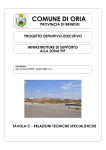
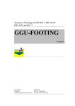
Figure 1 Consolidation layer
In Figure 1, a consolidation layer is shown, which can drain to the top and bottom. The pore water
pressure distribution is constant across the whole layer depth and corresponds to the surcharge
load p, which can be defined within the program. The program models the pore water pressure
distribution u across the layer depth in definable, constant, vertical steps, at user-defined times.
The area of the pore water pressure distributions is numerically integrated. By comparing this with
the constant pressure distribution in the unconsolidated state (t = 0), the degree of consolidation U
can be determined. The following is valid:
U
 u (t )  dx
s(t )
 1.0 
 u (t  0)  dx
s(t  )
A further term is the consolidation ratio Uz, which is defined as:
U z  1.0  u / um
where
u = pore water pressure
um = u / surcharge load
GGU-CONSOLIDATE User Manual
Page 10 of 71
April 2012
5.2
5.2.1
Numerical solution with difference equations
Fundamentals
In complete analogy to the above relationships, a numerical solution can also be modelled with
difference equations. The numerical solution offers no advantages for the system described in the
above figure, as generally more time will be needed to model the results. The uncontested advantages of the numerical solution for a consolidation problem can only be brought into play if a
system with more than one layer is being processed and/or if the pore water pressure distribution
at time t = 0 is not constant across the whole layer depth. The relationships used to solve the problem can be found in
 Braya M. Das (1983)
ADVANCED SOIL MECHANICS
McGraw-Hill
and are comprehensively described there. There is no need to ruminate on the derivations at this
point.
Difference equations are applied to the depth distribution of the pore water pressures as well as to
the time dimension. It is important to remember that the quality of the numerical solution is dependent upon the iteration size (small iterations = high precision but longer computing times). The
depth distribution steps for pore water pressures (z) can be user-defined. The time dimension
step t will be automatically selected by the program such that convergence is guaranteed. The
following is valid after Das with regard to the relationship of the normalised values z and t:
t / (z)² < 0.5
In the program, the stricter demand of 0.2 is implemented as opposed to 0.5.
5.2.2
Multi-layered system
When you investigate a multi-layered system with differing permeabilities or - strictly theoretically - differing consolidation coefficients CV, the program must always orient itself around the
larger permeability value with regard to defining the necessary time steps. As rapid changes in
pore water pressure can take place in layers with high permeability, a very small time step must be
selected in order to achieve sufficiently accurate results. If both low-permeability and highpermeability soils are present, long consolidation times are required. In extreme situations this can
lead to modelling times which, depending on the power of the computer used, can easily require
several days (!).
High-permeability soils require only small time steps.
Low-permeability soils require longer consolidation times.
For example, extreme modelling times may occur if you arrange a permeable sand layer (e.g.
k = 10-4 m/s) between two cohesive layers of low permeability (e.g. k = 10-9 m/s). In such systems
the sand layer can generally be neglected, unless it can drain externally to the system. In this case
it is simpler not to model this soil as sand, but instead to define boundary conditions for the sand
region with, e.g., a pore water pressure u = 0.
GGU-CONSOLIDATE User Manual
Page 11 of 71
April 2012
Before each computation commences, the program will estimate the expected modelling time; this
helps to visualise the problem of long modelling times. You can then attempt to reduce the modelling time by making sensible increases in the iteration steps (depth). But also remember that this
decreases the quality of the solution. You should also investigate the system with a view to possible simplifications. A permeable layer at the upper or lower system boundary can generally be
ignored. A permeable sand layer between two layers of low permeability also plays an important
role only if it can drain externally to the system under consideration (see above).
5.2.3
Continuous load application
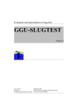
The previous explanations assume that the load is applied immediately. Generally, however, load
application is continuous during the construction phase of the structure. This effect can be considered by the program. To do this, define the load increase as a function of time using a polygon
course. A linear increase, for example, would then be converted to a step function. The type of
step function is dependent upon the times given by you for consolidation modelling.
100 %
Actual load increase
Step function
Selected consolidation times
Figure 2 Step function
If you would like a more precise approximation of the linear course, you need only donate a few
additional times in the load increase region when carrying out system input. The load increase
need not necessarily be defined as linear but can be entered as any polygon course. In previous
program versions only monotonic load increase was allowed. In the current version, modelling
with load decrease is also possible.
You will attain theoretically correct results if the consolidation coefficient Cv is the same
for load increase and decrease.
GGU-CONSOLIDATE User Manual
Page 12 of 71
April 2012
5.3
Consolidation settlements for non-linear compression
This approach is based on a suggestion by Prof. Dr.-Ing. Hartmut Schulz. The explanatory text
originates principally from Prof. Schulz.
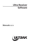
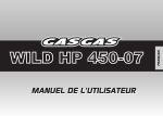
In Figure 3, this approach is demonstrated. Such representations are attained from the evaluation
of load-settlement tests. The GGU-OEDOM program allows such representations and test evaluations.
Normalspannung [kN/m²] (logarithmisch)
10
20
50
100
200
500
1000
0.50
Porenzahl [-]
0.40
0.30
0.20
0.10
0.00
Figure 3 Stress - pore ratio relationship (GGU-OEDOM program)
The initial assumption is of a linear reduction of the pore ratio e with the logarithm of the effective
vertical stress '. From this, the compression  is found by relating it to the total volume.
 ( z, t ) 
CC
 ' ( z , t )   ' ( z , t )
 ln(
1  e0 ( z )
 0' ( z )
 (z,t) = compression as a function of the location z and the time t
 CC = compression index
 e0(z) = pore ratio at z before loading
 0' (z) = stress at z before load increase
 0' (z,t) = compression change as a function of z and t
The effective vertical stresses as a function of the location z within the layer and the time t during
the consolidation process are already integrated into this equation. Furthermore, the fact that the
pore ratio changes linearly with the logarithm of the stress change is also considered. It follows
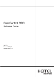
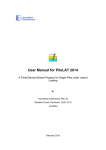
from this that the compression index CC is a constant. The evaluation in Figure 3 corresponds to
the example in Figure 4, which shows that in this case the compression index CC is almost constant across the complete stress region (CC  0.08). Only then can calculations be carried out using
this approach.
GGU-CONSOLIDATE User Manual
Page 13 of 71
April 2012
Normalspannung
[kN/m²]
(logarithmisch)
Normal
stress [kN/m²]
(logarithmic)
Kom press iocoeff
ns beicient
iw ert Cc
CC [--]]
Compession
0.14
10
20
50
100
20 0
500
1000
0.12
0.10
0.08
0.06
0.04
0.02
0.00
Figure 4 Stress - compression index relationship (GGU-OEDOM program)
The following input values are required for each layer:
 Compression index CC
 Pore ratio e0(top) = pore ratio e0 at top of layer
 Stress ' 0(top) = effective stress '0 at the top of the layer before loading
 Stress ' 0(bottom) = effective stress '0 at the bottom of the layer before loading
The program first determines the pore water pressure distribution u(t,z) at time t across the layer
depth z. The procedures described in Sections 5.1 and 5.2 are applied for this purpose. The stress
change is then calculated:
'(z,t) = 0'(z) + u(z,t)
0'(z) can be calculated from ' 0(top) and ' 0(bottom).
Further, the pore ratio e0(z) is computed from:
e0(z) = e0(top) + ln('0(top)/ 0'(z))·CC
We now have all variables to facilitate evaluation of the above equation.
 ( z, t ) 
CC
 ' ( z, t )   ' ( z, t )
 ln(
1  e0 ( z )
 0' ( z )
A dimensionless compression for the depth z is acquired for each time step. The integration of
these values across the depth provides the settlements(t).
D
s (t )    ( z , t )  dz
0
D = layer thickness
The equations described here are implemented in the program.
GGU-CONSOLIDATE User Manual
Page 14 of 71
April 2012
If you use the consolidation coefficient CV and the compression index CC in your calculations, the
program also provides a permeability determined using:
k
5.4
CV  CC   W
(1  e0 )   '
Analytical solution with vertical drainage
Besides classical consolidation theory, the program also commands cases in which consolidation
is accelerated by vertical drains (e.g. sand drains). These principles are also explained in Braya M.
Das (1983); Advanced Soil Mechanics; McGraw Hill.
Figure 5 Vertical drains
The honeycomb structure surrounding a drain can be converted to an equivalent circle, so that
axis-symmetrical consolidation modelling can be performed for each drain. In this case, according
to theory, dissipation of excess pore water pressure only occurs horizontal to the drains (axissymmetrical), so the drainage conditions at the top and base of the layer need not be given. However, the centres de of the drains and the radius rw of the drains must be given. In consolidation
layers with vertical drains the excess pore water pressure at any time is constant across the whole
layer depth. The excess pore water pressure is, however, variable as a function of the distance re
from the axis of the vertical drain. GGU-CONSOLIDATE determines the average pore water
pressure distribution.
GGU-CONSOLIDATE User Manual
Page 15 of 71
April 2012
5.5
Numerical solution with vertical drainage
In contrast to the analytical solution with vertical drainage, the numerical solution also allows
multi-layer systems, arbitrary pore water pressure distribution and load increase. Analytical methods with horizontal subdivisions, the spacing of which can be defined using the menu item
"Edit/System parameters", are used for modelling the numerical solution in accordance with the
previous sections. The consolidation degree U is then determined using numerical integration for
the given times.
5.6
Secondary settlements
Secondary settlements are the result of volume changes occurring under constant effective
stresses. Current scientific knowledge indicates that the increase in settlement with time is independent of the size of the effective stresses. The volume changes can be mathematically described
as follows (Garlanger, 1972):
e  e98  C  ln(t t 98 )
(1)
Where:
e
void ratio,
e98
void ratio for a degree of consolidation of 98%
(practical end of consolidation),
C
creep coefficient, relative to void ratio,
t
time from commencement of consolidation, t ≥ t98,
t98
time for a degree of consolidation of 98%,
from commencement of consolidation.
Secondary settlements are caused by viscous effects in the ground or porewater. The governing
laws were first reported by Buisman, 1936, based on settlement observations:
   98  C B  ln(
t
t 98
)
(2)
where:

compression,
98
compression for a degree of consolidation of 98%,
(practical end of consolidation),
CB
creep coefficient, relative to compression ,
t
time from commencement of consolidation, t ≥ t98,
t98
time for a degree of consolidation of 98%,
from commencement of consolidation.
It should be noted at this point that Equations (1) and (2) are used in the literature with both the
natural and the decadal logarithm. In practice the decadal logarithm appears to be in more widespread use than the natural logarithm.
GGU-CONSOLIDATE User Manual
Page 16 of 71
April 2012
The secondary settlements relevant for practical purposes are given by Equation (2) by integration
over the stratum thickness:
D
s sek (t )    98 dz  C B log  log(
0
t
t 98
D
)   dz
(3)
0
where:
ssek(t)
secondary settlements as a function of time t,
z
depth coordinate [m],
D
original stratum depth [m],
CBlog
creep coefficient, relative to compression  and
the decadal logarithm.
If integration is performed and the entire settlement process is adopted as a function of time, the
following expressions result:
s (t )  s (t )
s (t )  s (t 98 )  D  C B log  log(
t  t 98
t
t 98
)
t  t 98
(4)
with the additional variables:
s(t)
secondary settlements as a function of time t [m],
s(t)
consolidation settlements as a function of time t [m],
s(t98)
settlement as a result of consolidation and a degree of consolidation of 98% [m].
Strictly, secondary settlements commence together with consolidation settlements. They are allowed to begin later for analyses.
According to Kulhawy and Mayne, 1990, the ratio c/cc may lie between 0.04 and 0.06 for organic
soils: c can be interpreted as a compression index for secondary settlements and is a function of
the compression index for primary settlements. If the mean value of this ratio is adopted it may be
written as follows:
c (Ip) = 0.05  cc(Ip) bzw. c (wL) = 0.05  cc(wL)
(11)
This relationship also applies if the compression index is represented as a function of the water
content at the liquid limit. It gives the time-dependent secondary settlements by integrating the
change in void ratio e over the strata thickness d:
1
log(t d )
d
1  e s ( , t Kons )
0
s sek (t d , I p )  0.05  cc ( I p )  D  
GGU-CONSOLIDATE User Manual
Page 17 of 71
(12)
April 2012
Rough numerical values (abstract from TUM handouts by Prof. Vogt):
The following empirical values may be adopted in terms of secondary settlements: Cα < 0.005 for
overconsolidated clays, 0.005 < Cα < 0.05 for normally consolidated clays and 0.05 < Cα < 0.5
for organic and humous soils. Rheologically, soil creep is regarded as viscous behaviour.
If changes in relative settlements or vertical strains ε are described instead of the change in
void ratios, the Buisman factor CB (BUISMAN, 1936) is adopted instead of the creep factor Cα.
Where:
CB 

1   2

 ln t lnt 2   lnt1 
and
Cα = CB · (1 + e0)
A relationship exists between the Buisman constant CB and the compression index CC for primary
settlement via the toughness index lv where CB = CC · Iv /(1 + e).
The toughness index Iv correlates well with the water content at the liquid limit wL.
Iv [%] = -7.02 + 2.55 · ln (wL [%]).
A relationship also exists between creep velocities (compression rates) ε, reference times t (theoretical time since load application), toughness index Iv and effective stresses σ' (KRIEG 2000):
Iv
Iv
t 
 t  t0 
 0 '  0 

     1   
 1'  1 
 t0 
 t0 
Iv
In this context it is obvious that the creep velocities can be reduced by reducing the effective loads
and that compression rates are a function of both the stress levels and the time elapsed since the
load was applied.
KRIEG, S. (2000): Viskoses Verhalten von Mudden, Seeton und Klei. Heft 150, Veröff. Inst.
Bodenm. u. Felsm. Univ. Karlsruhe
GGU-CONSOLIDATE User Manual
Page 18 of 71
April 2012
Further reading:
Bjerrum, L.
1967 Engineering geology of Norwegian normally consolidated marine clays
as related to settlements of buildings. Seventh Rankine lecture.
Geotechnique, 17: 81-118
Buisman,
A.S.K.
1936 Results of long duration settlement tests. Proc. 1st ICSMFE, Cambridge, Mass., Vol.l:103-107
Crawford, C.B. 1964 Interpretation of the consolidation test,Journal of the Soil Mechanics
and Foundations Division, ASCE, 90: 87-102
Garlanger, J. E. 1972 The consoidation of soils exhibiting creep under constant effective
stress, Geotechnique 22, 71-78
Gudehus, G.,
1981 Bodenmechanik, Ferdinand Enke Verlag Stuttgart
Hvorslev, M.J., 1960 Physical Components of the Shear Strength of Saturated Clays,
Proceedings ASCE Research Conference on Shear Strength of
Cohesive Soils – Boulder, Colorado
Kulhawy, F.H., 1990 Manual on Estimating Soil Properties for Foundation Design,
Mayne, P.W.
EL-6800 Research Project 1493-6, prepared for Electric Power
Research Institute, 3412 Hillview Avenue, Palo Alto, California, 94304
Schulz, H.
2002 Setzungsprognosen für weiche Böden, Bauingenieur, Band 77,
September 2002, S. 407
Schulz, H.
2003 Prediction of Settlements of Soft Soils, Int. Workshop on Geotechnics
of Soft Soils-Theory and Practice. Vermeer, Schweiger, Karstunen &
Cudny (eds.)  2003 VGE
Stolle, D.F.E.,
Vermeer, P.A.,
Bonnier, P.G.
1999 A consolidation model for creeping clay, Can. Geotech. Journal,
36: 754-759
GGU-CONSOLIDATE User Manual
Page 19 of 71
April 2012
6 Short introduction using worked examples
6.1
Example system
The following system is given:
Layer A
Layer B
Figure 6 Example system
The unit weight of the embankment material is 19 kN/m³. The crown width is 5.0 m. The slopes
are inclined at 1 : 1.5. The following laboratory test values were determined for both consolidation
layers:
 Layer A
ES = 4 MN/m²
k = 1 · 10-8 m/s
 Layer B
ES = 2 MN/m²
k = 1 · 10-9 m/s
The maximum surcharge on the embankment is 5 · 19 = 95 kN/m². The system can drain to the top
and bottom. The settlement at time t =  is approx. 40 cm. The embankment is tipped in approx.
100 days. The question to be clarified is: at what point in time is 80 % of settlement achieved.
GGU-CONSOLIDATE User Manual
Page 20 of 71
April 2012
6.2
Test 1: Consolidation (analytical)
First, the system will be investigated using classical consolidation theory. As this is actually a twolayer system, we must simplify. The most brutal type of simplification is to model with a layer
thickness of 10.5 m, the smallest constrained modulus of ES = 2 MN/m² and the smallest permeability of k = 10-9 m/s.
Start the program. Select the menu item "File/New" or, if you already have a file loaded,
"Edit/Type of consolidation" and enter the preferences from the following dialogue box:
GGU-CONSOLIDATE User Manual
Page 21 of 71
April 2012
Select the menu item "Edit/System parameters" and enter the values from the following dialogue
box:
Select the menu item "Edit/Define times". The times given here are unsuitable for this problem,
as the consolidation time will certainly be more than 12 days for the current system. You can easily convince yourself of this by leaving the box with "Cancel" and selecting the menu item "System/Analyse" and then examining the temporal development of the degree of consolidation in the
diagram at the lower right. If necessary, use the zoom function to enlarge the diagram (menu item
"Graphics preferences/Zoom info"). Now return to this menu item. You can now individually
edit the times given in the input fields; this is simpler, however, with the "Generate" button.
GGU-CONSOLIDATE User Manual
Page 22 of 71
April 2012
Enter the values as shown in the dialogue box and confirm with "OK". Don't forget to activate the
"Quadratic" check box. Voila!
You have now generated a time series with a quadratic increase up to 901 days. Leave the dialogue box using "Done".
Now select the "System/Analyse" menu item. After a short time you will see the results. If everything has been entered correctly you can see from the time-settlement graphic at the lower right
that around 900 days are needed until 80% settlement has occurred. Alternatively, you can read
off the respective values from the table at the left page margin.
A 3-year embankment lying time would be unacceptable to the client. The system will therefore be
examined below in more detail.
GGU-CONSOLIDATE User Manual
Page 23 of 71
April 2012
6.3
Test 2: Consolidation (numerical)
With numerical consolidation, the two-layer system can be considered. Select the following preferences from the menu item "Edit/Type of consolidation":
The number of menu items in the "Edit" menu has increased. Select the menu item "Edit/System
parameters" and enter the data from the following dialogue box:
You can skip the menu item "Edit/Define times", as the same times as for Test 1 will be used.
Select the menu item "Edit/Soils". Enter the following values into the dialogue box and confirm
with "Done".
GGU-CONSOLIDATE User Manual
Page 24 of 71
April 2012
Select the menu item "Edit/Pore water pressure (max)", in order to enter the pore water pressure
distribution at the start of consolidation. Edit the number of stresses to 2 with the "x stress(es) to
edit" button. Then enter the values into the dialogue box.
You thus define a constant pore water pressure of 95.0 kN/m² across both layers. Now select the
menu item "System/Analyse". The program first performs an estimate of the modelling time required. If the forecast modelling time is greater than 5 seconds, a message box opens, allowing
you to start or abort the analysis. Information on reducing the modelling time is available by pressing the "Info" button. If you click "Yes", modelling follows. If everything has been entered correctly you can see from the time-settlement graphic at the lower right that around 350 days are
needed until 80% settlement has occurred. Alternatively, you can also read the respective values
from the table at the left page margin.
In contrast to the brutal forecast of 900 days in Test 1, this more sensitive investigation has
brought about a reduction in the lying time by a factor of approximately 3. The client, however, is
impatient and will still not accept an embankment lying time of around 1 year. The system will
therefore be examined below in even more detail.
GGU-CONSOLIDATE User Manual
Page 25 of 71
April 2012
6.4
Test 3: Consolidation (numerical) with real pore water pressure distribution
The assumption that the pore water pressure at time t = 0 is constant across the whole layer depth
is not exactly true. Because of the infinite extent of the embankment in section, lower pressures
result. In order to consider the real pore water pressure distribution, select the menu item
"Edit/Pore water pressure (max)" and then the "Generate" button. Enter the values into the
dialogue box.
The foundation width of 12.50 m is approximately the crown width of the embankment and half of
each slope width.
For "Distance foundation base - layer top [m]", the top of the uppermost consolidation
layer should always be taken as reference.
This is not necessarily ground level, but must be taken from the system to be investigated.
In this example, the top of the uppermost consolidation layer is 2.0 m below the embankment; you
must therefore enter a value of 2.0 for "Distance foundation base - layer top [m]". After confirming with "OK" the program models the stress distribution across the consolidation layers in
accordance with elastic-isotropic half-space theory.
GGU-CONSOLIDATE User Manual
Page 26 of 71
April 2012
Using the "Forward" button, navigate through the list to view the stresses at a depth of 10.5 m.
As an alternative to the automatic generation of pore water pressures you can, of course, also enter
the values manually.
Select the "System/Analyse" menu item. Evaluation of the analysis shows that the consolidation
time for 80% settlement has now been reduced to approx. 330 days, which is, of course, still not
satisfactory for the impatient client.
In the initial task formulation it was noted that the embankment tipping time was around 100 days.
The influence of this will now be investigated.
GGU-CONSOLIDATE User Manual
Page 27 of 71
April 2012
6.5
Test 4: Consolidation (numerical) with real pore water pressure distribution and
time-dependent loading function
It will be assumed that the 95 kN/m² surcharge is applied approximately linearly over a period of
100 days. In principal, the program can cope with any kind of stress increase. Select the menu
item "Edit/Load increase". Change the number of load increments to 2 and enter the values from
the following dialogue box.
For times which exceed the final time given here, a load component of 100% will always
be assumed, so that no further input is necessary.
Select the "System/Analyse" menu item. An evaluation of the analysis shows that the consolidation time until 80% settlement is achieved is now around 380 days. However, as this analysis also
includes the tipping time of 100 days, the lying time after completion of tipping is reduced to 280
days, which represents a gain of 50 days compared to the Test 3 model.
The client is still not satisfied with this. Luckily, however, drilling carried out in the meantime has
shown that there is a thin layer of sand between the two cohesive layers, which can drain laterally.
The influence this is investigated in Test 5 below.
GGU-CONSOLIDATE User Manual
Page 28 of 71
April 2012
6.6
Test 5: Consolidation (numerical) with real pore water pressure distribution and
time-dependent loading function and boundary condition
Under the assumption that the intercalated sand layer can take on a pore water pressure u = 0, the
system can be adjusted accordingly. Select the menu item "Edit/Boundary conditions" and set
the number of boundary conditions to 1. Then enter the following values:
This simulates a pore water pressure of "0" in the transition zone between the layers during consolidation.
Select the "System/Analyse" menu item. An evaluation of the analysis shows that the consolidation time until 80% settlement is achieved is now around 310 days. However, as this analysis also
includes the tipping time of 100 days, the lying time after completion of tipping is reduced to 210
days. The clients asks if it cannot be done quicker. Of course it can, but only using vertical drains
(see Test 6).
6.7
Test 6: Consolidation (analytical) with vertical drains
Select the menu item "Edit/Type of consolidation" and apply the following settings:
GGU-CONSOLIDATE User Manual
Page 29 of 71
April 2012
Consolidation modelling with vertical drains will first be performed on a one-layer system. It is
therefore necessary, as in Test 1, to simplify the current two-layer system to a system with one
layer. Select the menu item "Edit/System parameters" and enter the values from the following
dialogue box, similar to Test 1. Afterwards, analyse the system.
For drain centres of 1.5 m and a drain radius of 0.05 m the lying time is now only 50 days until
80% of settlements have occurred. The client is still not satisfied with this. So, last try!
GGU-CONSOLIDATE User Manual
Page 30 of 71
April 2012
6.8
Test 7: Consolidation (numerical) with vertical drains and actual pore water
pressure distribution and time-dependent loading function
In analogy to Test 6, a two-layer system will now be investigated. Select the following preferences
from the menu item "Edit/Type of consolidation":
In "Edit/System parameters", enter the following values:
Input for soil properties, pore water pressure distribution and load increases are analogous to Tests
2 to 4. The easiest way is to load the file for Test 4.
GGU-CONSOLIDATE User Manual
Page 31 of 71
April 2012
Boundary conditions can not be applied for numerical modelling of vertical drains.
The analysis shows that - after the tipping time of 100 days is complete - 80% of settlements have
occurred after a further lying time of only 10 days. This is still too long for the client.
Complete soil replacement is currently planned within the protection of a complex sheet pile wall
structure. The replacement material has a permeability of > 1 · 10-5 m/s. Apart from the substantial
reduction in absolute settlements, a projection of the time-settlement profile shows that 99% of
settlement has already occurred after approx. 2 hours. Can we live with this?
GGU-CONSOLIDATE User Manual
Page 32 of 71
April 2012
6.9
Test 8: Worked example with compression index CC
On the basis of Test 5 (see Section 6.6), time-settlement analysis with compression indices (see
Section 5.3) shall now be demonstrated. In addition to the values from Test 5, we need the following input data:
 Compression index CC
 Pore ratio e0(top) = pore ratio e0 at top of layer
 Stress '0(top) = effective stress '0 at the top of the layer before loading
 Stress '0(bottom) = effective stress '0 at the bottom of the layer before loading
The compression indices CC and the pore ratio e0(top) are known from load-settlement tests.
 Layer A
CC = 0.08
e0(top) = 0.42
 Layer B
CC = 0.11
e0(top) = 0.45
The stresses '0(top) and '0(bottom) prior to loading can be determined from the unit weights of the
individual layers and their thicknesses. We have the following unit weights:
Figure 7 Section of example system
 Sand
/ ' = 20/10 kN /m³
 Layer A
 ' = 8 kN /m³
 Layer B
 ' = 5 kN /m³
GGU-CONSOLIDATE User Manual
Page 33 of 71
April 2012
The groundwater level is at 1.0 m below the embankment formation level. This gives us the
following stress values:
 Layer A
'0(top) = 1.0 · 20.0 + 1.0 · 10.0 = 30 kN/m²
'0(bottom) = 30.0 + 4.0 · 8.0 = 62 kN/m²
 Layer B
'0(top) = 62 kN/m²
'0(bottom) = 62.0 + 6.5 · 5.0 = 94.5 kN/m²
Now enter the values from Test 5 or open the corresponding data record. Then select the menu
item "Edit/System parameters". Activate the button "With compression index Cc" and confirm
with "OK".
Select the menu item "Edit/Soils" and enter the following values:
GGU-CONSOLIDATE User Manual
Page 34 of 71
April 2012
Go to the "System/Analyse" menu item. The various result graphics are then displayed on the
screen, including the pore water pressure diagram.
Figure 8 Pore water pressure diagram test 8
Double-clicking in the diagram opens the editor box; here, you can select a visualisation using 101
days by pressing the "Select times" button. The effective stresses '0 are also displayed in the pore
water pressure diagram.
An evaluation of the analysis shows that the consolidation time until 80% settlement is achieved is
around 210 days. However, as this analysis also includes the tipping time of 100 days, the lying
time after completion of tipping is reduced to 110 days.
GGU-CONSOLIDATE User Manual
Page 35 of 71
April 2012
7 Description of menu items
7.1
7.1.1
File menu
"New" menu item
The desired solution method can be defined in a dialogue box. You will see the same dialogue box
by going to the "Edit/Type of consolidation" menu item.
In the dialogue box you define the unit of time to work with and whether the constrained modulus
is given as "kN/m²" or "MN/m²". If the "Include date with time if necessary" check box is activated the date can be displayed in the time axis in the subsequent evaluation diagram. The settlement period can thus be better visualised than when only a number of days are given.
Explanations of the consolidation types can be found in the "Preface" (see Section 1) and in the
"Theoretical principles" (see Section 5).
7.1.2
"Load" menu item
You can load a file with system data, which was created and saved at a previous sitting, and then
edit the system.
7.1.3
"Save" menu item
You can save data entered or edited during program use to a file, in order to have them available at
a later date, or to archive them. The data is saved without prompting with the name of the current
file. Loading again later creates exactly the same presentation as was present at the time of saving.
GGU-CONSOLIDATE User Manual
Page 36 of 71
April 2012
7.1.4
"Save as" menu item
You can save data entered during program use to an existing file or to a new file, i.e. using a new
file name. For reasons of clarity, it makes sense to use ".kon" as file suffix, as this is the suffix
used in the file requester box for the menu item "File/Load". If you choose not to enter an extension when saving, ".kon" will be used automatically.
7.1.5
"Printer preferences" menu item
You can edit printer preferences (e.g. swap between portrait and landscape) or change the printer
in accordance with WINDOWS conventions.
7.1.6
"Print and export" menu item
You can select your output format in a dialogue box. You have the following options:
 "Printer"
allows graphic output of the current screen contents. to the WINDOWS standard printer or
to any other printer selected using the menu item "File/Printer preferences". But you may
also select a different printer in the following dialogue box by pressing the "'Printer
prefs./change printer" button.
In the upper part of the dialogue box, the maximum dimensions which the printer can accept are given. Below this, the dimensions of the image to be printed are given. If the image is larger than the output format of the printer, the image will be printed to several pages
(in the above example, 4). In order to facilitate better re-connection of the images, the possibility of entering an overlap for each page, in x and y direction, is given. Alternatively,
you also have the possibility of selecting a smaller zoom factor, ensuring output to one
page ("Fit to page" button). Following this, you can enlarge to the original format on a
copying machine, to ensure true scaling. Furthermore, you may enter the number of copies
to be printed.
GGU-CONSOLIDATE User Manual
Page 37 of 71
April 2012
 "DXF file"
allows output of the graphics to a DXF file. DXF is a common file format for transferring
graphics between a variety of applications.
 "GGUCAD file"
allows output of the graphics to a file, in order to enable further processing with the
GGUCAD program. Compared to output as a DXF file this has the advantage that no loss
of colour quality occurs during export.
 "Clipboard"
The graphics are copied to the WINDOWS clipboard. From there, they can be imported
into other WINDOWS programs for further processing, e.g. into a word processor. In order
to import into any other WINDOWS program you must generally use the "Edit/Paste"
function of the respective application.
 "Metafile"
allows output of the graphics to a file in order to be further processed with third party software. Output is in the standardised EMF format (Enhanced Metafile format). Use of the
Metafile format guarantees the best possible quality when transferring graphics.
If you select the "Copy/print area" tool
from the toolbar, you can copy parts of
the graphics to the clipboard or save them to an EMF file. Alternatively you can send
the marked area directly to your printer (see "Tips and tricks", Section 8.3).
Using the "Mini-CAD" program module you can also import EMF files generated using other GGU applications into your graphics.
 "MiniCAD"
allows export of the graphics to a file in order to enable importing to different GGU applications with the Mini-CAD module.
 "GGUMiniCAD"
allows export of the graphics to a file in order to enable processing in the GGUMiniCAD
program.
 "Cancel"
Printing is cancelled.
GGU-CONSOLIDATE User Manual
Page 38 of 71
April 2012
7.1.7
"Batch print" menu item
If you would like to print several appendices at once, select this menu item. You will see the following dialogue box:
Create a list of files for printing using "Add" and selecting the desired files. The number of files is
displayed in the dialogue box header. Using "Delete" you can mark and delete selected individual
files from the list. After selecting the "Delete all" button, you can compile a new list. Selection of
the desired printer and printer preferences is achieved by pressing the "Printer" button.
You then start printing by using the "Print" button. In the dialogue box which then appears you
can select further preferences for printer output such as, e.g., the number of copies. These preferences will be applied to all files in the list.
7.1.8
"Exit" menu item
After a confirmation prompt, you can quit the program.
7.1.9
"1, 2, 3, 4" menu items
The "1, 2, 3, 4" menu items show the last four files worked on. By selecting one of these menu
items the listed file will be loaded. If you have saved files in any other folder than the program
folder, you can save yourself the occasionally onerous rummaging through various sub-folders.
GGU-CONSOLIDATE User Manual
Page 39 of 71
April 2012
7.2
7.2.1
Edit menu
"Project identification" menu item
You may enter a more detailed description of the system, which will be automatically entered into
the General legend (see Section 7.4.1).
7.2.2
"Type of consolidation" menu item
Using this menu item you can edit the default preferences of the current system. The dialogue box
corresponds to the box in the menu item "File/New" (see descriptions in Section 7.1.1).
GGU-CONSOLIDATE User Manual
Page 40 of 71
April 2012
7.2.3
"System parameters" menu item
7.2.3.1
Analytical methods
The governing system boundary conditions are entered using the menu item "Edit/System parameters". If you have chosen to use an analytical method to solve the problem, you will see the
following dialogue box (example):
Using classical consolidation
You must first enter the layer thickness and the load that initiates the consolidation process.
In order to properly model the temporal development of settlement, the consolidation coefficient
CV is required. This can be calculated from the constrained modulus ES and the permeability
coefficient k or be entered directly, if the value is known from oedometer tests. Enter your data
according to the activated check boxes.
GGU-CONSOLIDATE User Manual
Page 41 of 71
April 2012
Alternatively, the settlements can also be calculated using the compression index CC. Further information on this can be read by pressing the "Info" button after activating the "Use" compression
index CC check box. In the English-speaking world, in contrast to Germany, the compression
index CC is not defined to base loge, but to base log10. This can be specified here.
If a secondary settlement is adopted activate the "With secondary settlement" check box and
enter the soil parameter CB(log) (see "Theoretical principles/Secondary settlements" in Section 5.6).
For the "Classical consolidation (analytical)" you then define the drainage conditions (see lower
section of the above dialogue box). The number given after "No. of depth subdivisions" defines
the number of points at which the program determines the pore water pressure. Because the program performs an integration of the pore water pressures at these points to determine the degree of
consolidation, you should ensure that the number of subdivisions is not too small.
For a system utilising "Consolidation (analytical) with vertical drains", drainage is exclusively
horizontal, resulting in constant pore water pressures across the layer thickness for all time steps.
The "No. of depth subdivisions" in a system with vertical drains can therefore be defined using
the minimum value of "3", thereby reducing modelling time. For the same reason, layer thickness
does not influence the modelling results. It is only useful for the graphical representation of the
pore water pressure distribution.
It is not necessary to define drainage conditions in a system employing vertical drains. Instead of
the drainage conditions the "Vertical drainage geometry" group box is shown. Here, you define
the drain centres and the drain radius (also see Figure 5 in "Theoretical principles", Section 5.4).
Using consolidation with vertical drains
GGU-CONSOLIDATE User Manual
Page 42 of 71
April 2012
7.2.3.2
Numerical methods
If you chose to employ a numerical solution method, you need only select general boundary conditions in "Edit/System parameters". Input of soil properties can be carried out by going to the
"Edit/Soils" menu item (see Section 7.2.5). When you go to "Consolidation with both types
(numerical)", the following dialogue box opens
You must first enter the depth increment (difference equations). The proposed default value of
0.05 is generally sufficient for all but very thin layers. If you are unsure about the selected time
increment, repeat a previous calculation using either half or double the increment and then compare the two results. If the deviation is only minor, the selected time increment was sufficiently
small.
Here, you also specify whether modelling is carried out using the consolidation coefficient CV
and/or the compression index CC.
Define the drainage conditions and the dimensions of the vertical drains in the lower group box. If
you select one of the other numerical methods in the "Edit/Type of consolidation" menu item,
only the respective relevant group box ("Drainage conditions" or "Vertical drains") is displayed
in the above dialogue box.
If a secondary settlement is adopted activate the "With secondary settlement" check box. The
soil parameter CB(log) for the individual soil strata is entered using the menu item "Edit/Secondary
settlements" (see Section 7.2.10).
GGU-CONSOLIDATE User Manual
Page 43 of 71
April 2012
7.2.4
"Define times" menu item
This menu item allows you to define times for the consolidation analysis.
If you would like to edit the number of times used, press the "x times to edit" button and then
enter the new number of times. Use the "Sort" button to achieve ascending sorting of times. This
sorting is carried out automatically upon leaving the dialogue box, without the function being
explicitly called-up.
You can also use this function to eliminate a time from the table.
Simply assign the time to be eliminated a large value (e.g. 9999.0) and then click the
"Sort" button. The corresponding time is now the last time in the table and can be deleted
by reducing the number of times accordingly.
Using the "Generate" button you can easily generate a large number of new times applying a
predefined increase mechanism (also see the example in Test 1, Section 6.2).
GGU-CONSOLIDATE User Manual
Page 44 of 71
April 2012
7.2.5
"Soils" menu item
This menu item is only available for the numerical methods. The soil properties are entered
in "Edit/System parameters" when employing analytical methods.
First, define the number of soils in your system using the "x soil(s) to edit" button. Using the
"Sort" button, you can sort the soils according to depth; otherwise, sorting is carried out automatically upon leaving the dialogue box. To delete soil layers simply assign the soil a large depth
value (e.g. 99.0) and then press the "Sort" button. The corresponding soil is now at the end of the
table and can be deleted by reducing the number of soils accordingly.
If you activated neither "With consolidation coefficient Cv" nor "With compression index Cc"
in the "Edit/System parameters" menu item, you will see the following dialogue box.
The layer depths (base) are with reference to the top of the uppermost consolidation layer, as are
all other inputs. Furthermore:
 ES = constrained modulus of soil [kN/m²]
 k = permeability of soil [m/s].
You can alter the units for the constrained modulus to "kN/m²" in "Edit/Type of consolidation".
In order to allow modelling of the temporal development of settlement, the consolidation coefficient CV is required. This can be calculated from the constrained modulus ES and the permeability
coefficient k:
CV = ES · k / gamma(water)
Using the "Calculate" buttons it is possible to determine the constrained modulus or the value of k
for a given value of CV and to adopt this as the new parameter.
GGU-CONSOLIDATE User Manual
Page 45 of 71
April 2012
If you activated "With consolidation coefficient Cv" in the "Edit/System parameters" menu
item, enter the value of k and the consolidation coefficient into the slightly different dialogue box.
If you activated "With compression index Cc" in the "Edit/System parameters" menu item, the
soils dialogue box is expanded by the corresponding parameters. Depending on whether you are
also working with the consolidation coefficient CV, you will see the corresponding input boxes for
CV or constrained modulus and k (see the following example).
GGU-CONSOLIDATE User Manual
Page 46 of 71
April 2012
7.2.6
"Soils (reloading)" menu item
This menu item is only available if you have selected numerical methods and you are
working with a non-monotonous load increase.
In the dialogue box you define the ratio of the constrained modulus for reloading to the constrained modulus for initial loading for each type of soil. If you are working with the compression
index, define CC/CS accordingly.
7.2.7
"Pore water pressure (max)" menu item
This menu item is only active if you have selected one of the numerical methods.
If you would like to edit the number of stresses, select the "x stresses to edit" button and then
enter the new number of stresses. Using the "Sort" button, you can sort the stresses according to
depth. This sorting is carried out automatically upon leaving the dialogue box, without the function being explicitly called-up.
The layer depths (base) are with reference to the top of the uppermost consolidation layer, as are
all other inputs. You must also define the governing pore water pressures u corresponding to the
given depths.
The pore water pressure distribution can be saved to a ".kon_spg" file using the "Save" button; it
can be reloaded later using the "Load" button and thus be adopted for a different system.
GGU-CONSOLIDATE User Manual
Page 47 of 71
April 2012
A special delicacy here is the "Generate" button:
It allows you to generate the stress distribution of any footing foundation at either the characteristic point or at the foundation centre. The "Increment (depth)" input specifies the dept subdivisions at which the stresses are calculated. If the footing is located above the consolidating layer,
specify the distance in "Distance foundation base-layer top [m]".
7.2.8
"Boundary conditions" menu item
This menu item is only active if you have selected "Classical consolidation (numerical)"
as the consolidation type.
If there are permeable layers within the system which can drain externally, it is possible to use this
menu item to take this influence into consideration by means of boundary conditions (also see
"Theoretical principles", Section 5.2.2).
Enter the depth and the respective pore water pressure, which will then be kept constant for a
subsequent analysis for the entire duration of consolidation.
GGU-CONSOLIDATE User Manual
Page 48 of 71
April 2012
7.2.9
"Load increase" menu item
This menu item is only active if you have selected one of the numerical methods.
Consideration of a continuous load application during a structure's entire manufacturing phase can
be achieved using this menu item. Using the "x load increments to edit" button in the following
dialogue box you first define the number of load increases.
The load increase need not necessarily be defined as linear but can be entered as any kind of polygon course. Define the time and corresponding percentage load increase. It is also possible to
model a load decrease.
A given, repetitive load pattern can be automatically created using the "Repeat" button. This makes it unnecessary to enter the entire sequence using individual values.
For long consolidation periods it may be useful to define the load increase by specifying dates (see
the "Example with date.kon" file). Click the "Switch to entering "Time as date"" button. The
previously entered times are automatically converted to the start date (see dialogue box "File/New", Section 7.1.1). After changing the button reads "Switch to entering "Time as number"". It is possible to change back to entering the loads in the selected time units, e.g. in days, by
clicking the button.
GGU-CONSOLIDATE User Manual
Page 49 of 71
April 2012
The defined load increase is converted to a step function. The exact form of the step function
depends on the time steps selected for use in the consolidation analysis (see menu item
"Edit/Define times", Section 7.2.4).
100 %
Actual load increase
Step function
Selected consolidation times
The more consolidation times are defined in the region of the load increase, the more precise will
be the approximation of the real function to the step function.
7.2.10
"Secondary settlements"
This menu item is only active if you have selected one of the numerical methods.
If secondary settlements are activated in the system data the following dialogue box opens via this
menu item:
The respective soil parameter CB(log) for the soil strata can be defined here (see "Theoretical principles/Secondary settlements" in Section 5.6).
GGU-CONSOLIDATE User Manual
Page 50 of 71
April 2012
7.2.11
"Installation time (vertical drains)" menu item
This menu item is only active if you have selected "Consolidation with both types (numerical)" as the consolidation type.
You must define the installation time of the vertical drains. The time from which the vertical
drains are incorporated in the analysis is marked in the evaluation diagrams.
7.2.12
"cv(axial)/cv" menu item
This menu item is only active if you have selected "Consolidation with both types (numerical)" as the consolidation type.
You define the ratio of the consolidation coefficients CV (axial)/CV .
7.3
7.3.1
System menu
"Analyse" menu item
This starts the analysis. Alternatively, press the [F5] function key or click on the Calculator in the
tool bar. If you have specified particular settings for the system the program notified you of these
settings before analysis begins. The program first performs an estimate of the modelling time
required. If the forecast modelling time is greater than 5 seconds, a message box opens, allowing
you to start or abort the analysis. Information on reducing the modelling time is available by pressing the "Info" button. If you click "Yes", modelling follows. Once complete, the modelled system
is displayed.
GGU-CONSOLIDATE User Manual
Page 51 of 71
April 2012
7.4
7.4.1
Output preferences menu
"General legend" menu item
A legend with general properties will be displayed on your output sheet if you have activated the
"Show legend" check box. Using this menu item you can alter the type of presentation.
You can edit the legend "Heading" at will. The position of the legend can be defined and edited
using the values "x value" and "y value". You control the size of the legend using "Font size" and
"Max. no. of lines"; where necessary, several columns are used.
The fastest way to modify the position of the legend is to press the [F11] function key and
then to pull the legend to the new position with the left mouse button pressed.
The file name can be switched off ("None" option button) or be displayed automatically with or
without the path by selecting the appropriate "Short" or "Long" option button.
Any project identification entered (see Section 7.2.1) will also be shown in the general legend.
GGU-CONSOLIDATE User Manual
Page 52 of 71
April 2012
7.4.2
"Pore water pressure/consolidation ratio" menu item
If you activate the "Show pore water pressure/consolidation ratio" check box in the dialogue
box for this menu item, your output sheet will display a graphical representation of the pore water
pressure profile across the depth, or the consolidation ratio (see "Theoretical principles"). A
variety of settings are available in the dialogue box, depending on the type of consolidation selected and the system defaults.
You can define and edit position and size of the graphics by editing the values "x" and "y", and
"Width" and "Height". You can also edit these values from within the screen presentation by
pressing the [F11] function key (see Section 7.4.10).
With the help of the combi-box below "X axis as:", the representation of the x-axis can be
switched from pore water pressure in [kN/m²] or [MN/m²] to a representation as the dimensionless
consolidation ratio UZ. The calculated pore water pressures can also be saved as an ASCII file.
Here, you can define the time up to which the values are saved in the dialogue box.
GGU-CONSOLIDATE User Manual
Page 53 of 71
April 2012
The "Select times" button activates the following dialogue box where you can select those of the
defined times to be displayed in the pore water pressure distribution or consolidation ratio graphics.
All times are activated by pressing the "All" button. All times are deactivated by pressing the
"None" button. This selection is particularly useful because as many points (times) as possible
should be used in order to achieve a continuous smooth course in the graphical representation of
the temporal development of the consolidation degree. However, too many distribution lines disturb the graphical representation of pore water pressure profiles, as they often merge into one
another. If the "Times as date" check box in the above dialogue box is activated, the date for the
respective consolidation period is shown instead of the time in the selected units.
If vertical drains are subsequently installed (consolidation type "Numerical consolidation with
both drain types") the installation time can also be marked in the specified colour in the active
"Times" group box.
If you activate the "Show pore water pressure/consolidation ratio" check box the distribution
lines are labelled with either the "Times" or the auxiliary value "TV". TV is defined as
TV = CV / H² · t
CV = consolidation coefficient = k · ES/W
H = layer thickness
t = time
Representation of the curve by means of "TV" is generally only useful when re-modelling
standardised curves from the literature.
For long consolidation periods it may be useful to label the time axis with the date instead of days
or another defined time unit (see the "Example with date.kon" file). Activate the "Times as
date" check box to enable this option. The date function must be activated in the "File/New" or
"Edit/Type of consolidation" menu item dialogue boxes to use this function (see Section 7.1.1). It
is also possible to define the diagram "Font size" and user-defined axes values. The "Max. ratio"
of the x- and y-axes are defined after clicking "Define axes".
GGU-CONSOLIDATE User Manual
Page 54 of 71
April 2012
If you activate the "Show soil layers" check box, the current soil sequence is displayed in the
graphics. This check box is only available when using a numerical method. When modelling with
the compression index CC a number of selections affecting the representation can be made in the
lower group box.
7.4.3
"Time-settlement" menu item
If you activate the "Show time-settlement" check box in the dialogue box for this menu item, the
temporal profile of the degree of consolidation is displayed on the screen.
You can define and edit position and size of the graphics by editing the values "x" and "y", and
"Width" and "Height". You can also edit these values from within the screen presentation by
pressing the [F11] function key (see Section 7.4.10).
If the "Vertical axis from top to bottom" check box is activated, representation is reversed with
regard to the normal representation of settlements. Using the "Dimensionless time axis as TV"
check box it is possible to switch representation of the time axis to dimensionless TV values. This
is generally only useful when re-modelling standardised curves from the literature.
GGU-CONSOLIDATE User Manual
Page 55 of 71
April 2012
You can indicate your selected times with a marker; the size, colour and shape of the marker can
be specified in a dialogue box by pressing the "Marker" button. Alternatively, you can choose
user-defined axes or a logarithmic time axis. If the labelling of the time axis is too tight, you can
edit the units of time in the "Edit/Type of consolidation" menu item (see Section 7.1.1). If the
date function is also activated, additional labelling with the date can be achieved in the timesettlement diagram by activating the "Time axis with date" check box.
In the "Vertical axis as" group box you define the variable to be drawn versus the time axis. This
also activates further fields for specifying preferences with regard to the selected variable, depending on the chosen representation. In the above dialogue box the "Settlement [cm]" option button
is activated. So the "Measured settlements" group box is also active and you can display individual measured values, for example measured at on-site settlement gauges, in addition to the calculated settlement curve. The additional measured values are entered into a separate dialogue box
which opens after you click the "Edit" button. If pore water pressure visualisation is active the
pore water pressure values calculated for a given depth can be saved in an ASCII file.
Further graphic elements can be activated at the bottom of the dialogue box; the time-settlement
area can be colour-backed, for example. If you have defined a load increase, the step function on
which modelling is based can be displayed in the graphics by activating the "Show load curve"
check box. This makes a separate representation of the load curve unnecessary (see Section 7.4.7).
Preferences can be defined for the pen colour and width in the menu item "Graphics preferences/Pen colour and width" (see Section 7.5.5). If vertical drains are subsequently installed
(consolidation type "Numerical consolidation with both drain types") the installation time can
also be marked in the specified colour.
7.4.4
"System presentation" menu item
The current system is displayed in the graphics when you activate the "Show system" check box.
The format and appearance of the graphics can be altered using this menu item.
You can define and edit position and size of the graphics by editing the values "x" and "y", and
"Width" and "Height". You can also edit these values from within the screen presentation by
pressing the [F11] function key (see Section 7.4.10).
If you have selected a numerical method for the type of consolidation, you can label the system
diagram with the soil names at the desired position (see dialogue box above).
GGU-CONSOLIDATE User Manual
Page 56 of 71
April 2012
7.4.5
"Output table" menu item
In addition to graphically representing the temporal profile of the degree of consolidation, a table
(output table) containing the degree of consolidation is also displayed if the "Show output table"
check box is activated in the dialogue box. The settlements can also be shown in the output table.
You can define and edit position and size of the table by editing the values "x" and "y", and
"Width" and "Height". You can also edit these values from within the screen presentation by
pressing the [F11] function key (see Section 7.4.10). The font size used for the output table entries
is automatically adapted by the program to suit the size of the table.
By default, the output table also uses the dimensionless time value TV. The TV entry can be suppressed by deactivating the "Output table with TV" check box. Further entries can also be
adopted for the output table. In addition, it is possible to save the output table by clicking the
"Save values as ASCII file" button.
GGU-CONSOLIDATE User Manual
Page 57 of 71
April 2012
7.4.6
"Soil properties legend" menu item
This menu item is only active if you have selected one of the numerical methods.
A legend containing the soil properties is displayed with the graphics. If the "Show legend" check
box is activated you can edit the legendrepresentation in the dialogue box for this menu item.
You can define and edit the position of the legend using the values "x" and "y". The size of the
legend is controlled by the values for "Font size". The fastest way to modify the position of the
legend is to press the [F11] function key and then to pull the legend to the new position while
holding the left mouse button.
If "System coloured" is activated in the combi-box, the soils will be displayed coloured both in
the soil properties legend and in the system graphics (see Section 7.4.4). You can also define either hatching or colour fill and hatching for the different soil types in the combi-box. If you select
"System without all", the soils are merely numbered. The depths of the individual soil layers are
shown in the legend if the "With depths" check box is activated. The required settings can be
made in the "Soil colours + hatching" group box:
 "Automatic"
The soils are assigned soils colours automatically by the program. If the check box is not
selected, the soil colours individually defined using the "Soil colours" button will be adopted.
 "Soil colours"
You will see a dialogue box, in which you can define your preferences. After clicking the
button with the desired number you can assign each soil layer a new number or reorganise
using the "Soil colours/Reorganise" command button. You can save your colour preferences to a file with "Soil colours/Save" and use them for different systems by means of the
"Soil colours/Load" command button. In the lower group box you can also transfer the
colour preferences to the Windows colour management dialogue box, or vice versa, as
user-defined colour preferences for example. You can read a further description by pressing the "Info" button.
GGU-CONSOLIDATE User Manual
Page 58 of 71
April 2012
 "Hatching"
Opens a dialogue box in which you can define different hatching for each soil.
 "Legend hatching factor"
Input here allows tighter hatching in the soil legend. Input < 1.00 can be useful if the hatching spacing is so large that the differences in the hatching of individual soils can no longer
be properly discerned in the relatively small boxes used in the legend.
7.4.7
"Load curve" menu item
If you have defined a load increase, the load curve can be displayed in the graphics. In addition to
the actual load curve, the step function used as the basis for modelling, resulting from the userdefined consolidation times, is also represented. If the "Show load curve" check box is activated
you can edit the representation in the dialogue box for this menu item.
You can define and edit position and size of the graphics by editing the values "x" and "y", and
"Width" and "Height". You can also edit these values from within the screen presentation by
pressing the [F11] function key (see Section 7.4.10).
A logarithmic time axis or an additional date display on the time axis can be activated. The date
function must be activated in the "File/New" or "Edit/Type of consolidation" menu item dialogue
boxes for this (see Section 7.1.1). Alter the axes selected by the program using the "Define axes"
button. In the subsequent dialogue box you specify the times and load values as minimum and
maximum values to be used for the x- and y-axes.
The "Load curve with colour" check box activates a colour-backing in the specified colour for
the load area. Preferences can be defined for the pen colour and width in the menu item "Graphics preferences/Pen colour and width" (see Section 7.5.5). If vertical drains are subsequently
installed (consolidation type "Numerical consolidation with both drain types") the installation
time can also be marked in the specified colour.
GGU-CONSOLIDATE User Manual
Page 59 of 71
April 2012
7.4.8
"Pore ratio diagram" menu item
This menu item is only active if you have selected Compression index CC for the settlement analysis (see menu item "Edit/System parameters", Section 7.2.3).
If the "Show pore ratio diagram" check box is activated you can edit the graphical representation
in the dialogue box for this menu item.
You can define and edit the position of the graphics by editing the values "x" and "y", and
"Width" and "Height". You can also edit these values from within the screen presentation by
pressing the [F11] function key (see Section 7.4.10). The background colour of the legend can be
altered.
By pressing the "Marker" button a further dialogue box opens allowing you to define the size,
colour and shape of the marker (e.g. triangle, rectangle, circle) according to your wishes. In order
to suppress a representation with markers, deactivate the "Pore ratio diagram with markers"
check box in this dialogue box.
GGU-CONSOLIDATE User Manual
Page 60 of 71
April 2012
7.4.9
"Page size and margins" menu item
The default page set-up is A3 when the program is started. You can edit the page format in the
following dialogue box.
 "Page in general" defines the size of the output sheet. The A3 format is set as default. The
program automatically draws thin cutting borders around the page, which are required
when using a plotter on paper rolls. The borders can be switched off using the menu item
"Graphics preferences/With borders" (see Section 7.5.4).
 "Page margins" defines the position of a frame as a distance to the margins. This frame
encloses the subsequent diagram.
7.4.10
"Move objects" menu item
When you go to this item you can move the various objects and legends with the aid of the mouse.
Move the mouse over the object to be moved. When you are located above a moveable object the
mouse pointer appears in the shape of a cross. You can now press and hold the left mouse button
and drag the object to the required position.
After going to this menu item only one object at a time can be moved using the mouse or
its size be altered.
In order to move or edit several objects, this function can be more quickly activated by
pressing [F11] or the
icon.
The size of an object can also be altered using this menu item or the [F11] key. If you move over
the frame of a changeable object after activating this function the mouse assumed the shape of a
double-headed arrow. Hold the left mouse button and move the frame until the element has
reached the required size. To retain the ratio of the sides, pull at one corner only. If on one side
only is pulled the object will become higher or wider.
GGU-CONSOLIDATE User Manual
Page 61 of 71
April 2012
7.5
7.5.1
Graphics preferences menu
"Refresh and zoom" menu item
The program works on the principle of What you see is what you get. This means that the screen
presentation represents, overall, what you will see on your printer. In the last consequence, this
would mean that the screen presentation would have to be refreshed after every alteration you
make. For reasons of efficiency and as this can take several seconds for complex screen contents,
the screen is not refreshed after every alteration.
If, e.g., after using the zoom function (see below), only part of the image is visible, you can
achieve a complete view using this menu item.
A zoom factor between 0.4 and 8.0 can be entered in the input box. By then clicking on "Use" to
exit the box the current factor is accepted. By clicking on the "0.4", "0.6", etc. buttons, the selected factor is used directly and the dialogue box closed.
It is much simpler, however, to get a complete overview using [Esc]. Pressing [Esc] allows a complete screen presentation using the zoom factor specified in this menu item. The [F2] key allows
screen refreshing without altering the coordinates and zoom factor.
7.5.2
"Zoom info" menu item
By clicking two diametrically opposed points you can enlarge a section of the screen in order to
view details better. An information box provides information on activating the zoom function and
on available options.
7.5.3
"Legend font selection" menu item
With this menu item you can switch to a different true-type font. All available true-type fonts are
displayed in the dialogue box.
7.5.4
"With borders" menu item
The program automatically draws thin cutting borders around the page, which are required when
using a plotter on paper rolls. The borders can be switched on or off using this menu item(see also
menu item "Output preferences/Page size and margins", Section 7.4.9).
GGU-CONSOLIDATE User Manual
Page 62 of 71
April 2012
7.5.5
"Pen colour and width" menu item
In order to enhance the clarity of the graphics you can edit the pen settings for various graphical
elements.
You can edit the pen widths and types for the elements shown in the dialogue box; by clicking on
the button with the element designation you can also edit the pen colours. The vertical and horizontal auxiliary lines form the mesh in the graphical representation of the pore water pressure
profile and the degree of consolidation.
On monochrome printers (e.g. laser printers), colours are shown in a corresponding grey scale.
Graphic elements employing very light colours may be difficult to see. In such cases it makes
sense to edit the colour preferences.
7.5.6
"Mini-CAD toolbar" menu item
Using this menu item you can add free text to the graphics and add lines, circles, polygons and
images (e.g. files in formats BMP, JPG, PSP, TIF, etc.). A pop-up menu opens, the icons and
functions used are described in more detail in the Mini-CAD manual provided.
Objects created with the "Mini-CAD" tool are based on the page format (in mm). This makes you
independent of the coordinate system and keeps you in the same position on the page. You should
select the "Mini-CAD toolbar" if you wish to place general information on the drawing (company
logo, report numbers, plan numbers, stamp etc.). Once you have saved the header information to
disk (see Mini-CAD user manual), you can load it into completely different systems (with different system coordinates). The saved header information will appear in exactly the same position on
the page, which greatly simplifies the creation of general page information
GGU-CONSOLIDATE User Manual
Page 63 of 71
April 2012
7.5.7
"Toolbar preferences" menu item
After starting the program a horizontal toolbar appears below the program menu bar. If you would
rather work with a popup window with several columns, you can specify your preferences using
this menu item. The smarticons can also be switched off.
At the bottom of the program window you find a status bar with further information. You can also
activate or switch off the status bar here. The preferences will be saved in the "GGUCONSOLIDATE.alg" file (see menu item "Graphics preferences/Save graphics preferences")
and will be active at the next time the program is started.
By clicking on the tools (Smarticons) you can directly reach most of the program functions. The
meaning of the Smarticons appears as a text box if you hover with the mouse pointer over the
tools. Some of the tool functions can be activated from the normal menu items.
"Zoom out"
If you have previously zoomed in, this tool returns to a full screen display.
"Zoom (-)"/"Zoom (+)"
With the zoom functions you can zoom in or out of parts of the image, by clicking the left mouse
button.
"Undo move object"
By clicking this icon the last performed movement of graphical elements made using the [F11]
function key or the menu item "Output preferences/Move objects" can be undone.
"Restore move object"
By clicking this symbol, the last object movement undo carried out using "Undo move object"
can be restored.
"Copy/print area"
Use this tool to copy only parts of the graphics in order to paste them, e.g. to a report. You will see
information on this function and can then mark an area, which is copied to the clipboard or can be
saved in a file. Alternatively you can send the marked area directly to your printer (see "Tips and
tricks", Section 8.3).
"Colour on/off"
If you need to remove the colour from the system presentation, to create a black and white printout, for example, use this on/off switch.
GGU-CONSOLIDATE User Manual
Page 64 of 71
April 2012
7.5.8
"Load graphics preferences" menu item
You can reload a graphics preferences file into the program, which was saved using the "Graphics preferences/Save graphics preferences" menu item. Only the corresponding data will be
refreshed.
7.5.9
"Save graphics preferences" menu item
Some of the preferences you made with the menu items of the "Graphics preferences" menu can
be saved to a file. If you select "GGU-CONSOLIDATE.alg" as file name, and save the file on
the same level as the program, the data will be automatically loaded the next time the program is
started and need not be entered again.
If you do not go to "File/New" upon starting the program, but open a previously saved file
instead, the preferences used at the time of saving are shown. If subsequent changes in the
general preferences are to be used for existing files, these preferences must be imported using the menu item "Graphics preferences/Load graphics preferences".
GGU-CONSOLIDATE User Manual
Page 65 of 71
April 2012
7.6
7.6.1
? menu
"Copyright" menu item
You will see a copyright message and information on the program version number.
The "System" button shows information on your computer configuration and the folders used by
GGU-CONSOLIDATE.
7.6.2
"Help" menu item
The GGU-CONSOLIDATE manual is opened as a PDF document. The help function can also be
accessed using the [F1] function key.
7.6.3
"GGU on the web" menu item
Using this menu item you can access the GGU Software website: www.ggu-software.com.
Keep in touch with new program versions and the regular download offers.
If you would like to be automatically notified about program innovations, please register for the
Newsletter in our Knowledge Base. Go to the following website: http://kbase.civilserve.com.
7.6.4
"GGU support" menu item
This menu item takes to the GGU-Software Support area at www.ggu-software.com.
7.6.5
"What's new?" menu item
You will see information on program improvements in comparison to older versions.
7.6.6
"Language preferences" menu item
This menu item allows you to switch the menus and the graphics from German to English and vice
versa. To work in German, deactivate the two check boxes "Dialoge + Menüs übersetzen (translate dialogues, menus)" und "Graphiktexte übersetzen (translate graphics)".
Alternatively, you can work bilingually, e.g. with German dialogue boxes but with graphic output
in English. The program always starts with the language setting applicable when it was last ended.
GGU-CONSOLIDATE User Manual
Page 66 of 71
April 2012
8 Tips and tricks
8.1
Keyboard and mouse
You can scroll the screen with the keyboard using the cursor keys and the [Page up] and [Page
down] keys. By clicking and pulling with the mouse, with [Ctrl] pressed, you activate the zoom
function, i.e. the selected section will fill the screen. Furthermore you can use the mouse wheel to
zoom in/out or scrolling the screen presentation. The following mouse wheel functions are
available:
 Mouse wheel up
= move screen image up
 Mouse wheel down
= move screen image down
 [Ctrl] + mouse wheel up
= enlarge screen image (zoom in)
 [Ctrl] + mouse wheel down
= shrink screen image (zoom out)
 [Shift] + mouse wheel up
= move screen image right
 [Shift] + mouse wheel down
= move screen image left
If you click the right mouse button anywhere on the screen a context menu containing the principal menu items opens.
By double-clicking the left mouse button on legends or Mini-CAD objects, you will immediately
move to the editor for the selected object and can then edit it.
GGU-CONSOLIDATE User Manual
Page 67 of 71
April 2012
8.2
Function keys
Some of the function keys are assigned program functions. The allocations are noted after the
corresponding menu items. The individual function key allocations are:
 [Esc] refreshes the screen contents and sets the screen back to the given format. This is
useful if, for example, you have used the zoom function to display parts of the screen and
would like to quickly return to a complete overview.
 [F1] opens the manual file.
 [F2] refreshes the screen without altering the current magnification.
 [F3] opens the menu item "Edit/System parameters".
 [F5] opens the menu item "System/Analyse".
 [F11] activates the menu item "Output preferences/Move objects".
8.3
"Copy/print area" icon
A dialogue box opens when the "Copy/print area" icon
in the menu toolbar is clicked, describing the options available for this function. For example, using this icon it is possible to either
copy areas of the screen graphics and paste them into the report, or send them directly to a printer.
In the dialogue box, first select where the copied area should be transferred to: "Clipboard",
"File" or "Printer". The cursor is displayed as a cross after leaving the dialogue box and, keeping
the left mouse button pressed, the required area may be enclosed. If the marked area does not suit
your requirements, abort the subsequent boxes and restart the function by clicking the icon again.
If "Clipboard" was selected, move to the MS Word document (for example) after marking the
area and paste the copied graphics using "Edit/Paste". If "File" was selected, the following dialogue box opens once the area has been defined:
The default location of the file is the folder from which the program is started and, if several files
are created, the file is given the file name "Image0.emf" with sequential numbering. If the
"Rename" button in the dialogue box is clicked, a file selector box opens and the copied area can
be saved under a different name in a user-defined folder. Saving can be aborted by pressing the
"Delete" button.
If the "Printer" button was pressed in the first dialogue box, a dialogue box for defining the
printer settings opens after marking the area. Following this, a dialogue box for defining the image
output settings opens. After confirming the settings the defined area is output to the selected
printer.
GGU-CONSOLIDATE User Manual
Page 68 of 71
April 2012
9 Index
Analysis, start/abort.......................................... 51
ASCII file export, calculated pore water
pressures....................................................... 53
ASCII file export, output table ......................... 57
ASCII file export, pore water pressure
at selected depth ........................................... 56
DIN 4019 ............................................................ 5
Drainage conditions, consider during
consolidation .................................................. 9
Drainage conditions, define for analytical
methods ........................................................ 42
Drainage conditions, define for numerical
methods ........................................................ 43
DXF file, export................................................ 38
DXF file, import ................................................. 6
B
E
Boundary conditions, define....................... 29, 48
Elastic-isotropic half-space theory ................... 26
EMF format ...................................................... 38
A
C
Calculation, pore ratio ...................................... 14
Calculation, stress change................................. 14
CB(log), for secondary settlements ...................... 17
Clipboard .......................................................... 38
CodeMeter stick.................................................. 7
Colours of soil layers, define............................ 58
Colours of soil layers, switch on/off................. 64
Colours/pens, define for graphical elements..... 63
Company logo, add via Mini-CAD .................. 63
Compression index, as result from
Oedometer test ............................................. 13
Compression index, soil properties input
if activated.................................................... 46
Consolidation coefficients, calculation............... 9
Consolidation coefficients, define ratio ............ 51
Consolidation modelling, axis-symmetrical ..... 15
Consolidation ratio, definition .......................... 10
Consolidation times, define unit ....................... 36
Consolidation times, define/delete.................... 44
Consolidation times, generate........................... 22
Consolidation times, select for display ............. 54
Consolidation types, description......................... 5
Consolidation types, select ............................... 36
Constrained modulus, define for analytical
methods ........................................................ 41
Constrained modulus, define for numerical
methods ........................................................ 45
Constrained modulus, define unit ..................... 36
Constrained modulus, in calculation................... 9
Context menu, open.......................................... 67
Copy/print area ..................................... 38, 64, 68
Creep coefficient, for secondary settlements.... 17
Cutting borders, switch on/off .......................... 62
D
Darcy's Law, application to consolidation.......... 9
Degree of consolidation, determination............ 10
Deleting, soil layers .......................................... 45
Deleting, times.................................................. 44
Depth subdivisions, define ............................... 42
Difference equations, application ..................... 11
Difference equations, define
depth increments .......................................... 43
Differential equation, consolidation ................... 9
GGU-CONSOLIDATE User Manual
F
File, display name in legend ............................. 52
File, load/save................................................... 36
Font selection.................................................... 62
Forecast, modelling time .................................. 12
Function keys ................................................... 68
Further reading, secondary settlements ............ 19
G
General page informations, add via
Mini-CAD .................................................... 63
GGUCAD file, export....................................... 38
GGUMiniCAD file, export ............................... 38
Graphics, add via Mini-CAD............................ 63
H
Hatching of soil layers, define .......................... 59
Hooke's Law, application to consolidation ......... 9
I
Installation .......................................................... 7
Installation time, define for vertical drains ....... 51
Installation time, mark in load curve legend..... 59
Installation time, mark in output table .............. 57
Installation time, mark in pore water
pressure/consolidation ratio graphics ........... 54
Installation time, mark in time-settlement
graphics ........................................................ 56
Iteration steps, influence on calculation ........... 11
K
Knowledge Base, access................................... 66
L
Labelling, tight time axis .................................. 56
Language preferences ....................................... 66
Layout, define for page..................................... 61
Layout, edit for general legend......................... 52
Layout, edit for load curve legend.................... 59
Page 69 of 71
April 2012
Layout, edit for output table ............................. 57
Layout, edit for pore ratio diagram................... 60
Layout, edit for pore water pressure/
consolidation ratio graphics ......................... 53
Layout, edit for soil properties legend.............. 58
Layout, edit for system graphics....................... 56
Layout, edit for time-settlement graphics ......... 55
Legend, alter position/size using mouse ........... 61
Licence protection .............................................. 7
Load application, continuous............................ 12
Load curve, activate legend display ................. 59
Load curve, display in time-settlement
graphics ........................................................ 56
Load increase, step function ............................. 12
Load increase/decrease, define ................... 28, 49
Load-settlement test, result representation ....... 13
M
Metafile, export ................................................ 38
Mini-CAD file, export ...................................... 38
Mini-CAD, use ................................................. 63
Modelling time, for multi-layered system ........ 11
Modelling time, reducing ................................. 51
Mouse click functions....................................... 67
Mouse wheel functions..................................... 67
Multi-layered system, notes for calculation...... 11
O
Objects, alter position/size using mouse........... 61
Oedometer test, result representation................ 13
Output table, activate display ........................... 57
P
Page format, define........................................... 61
Page margins, define ........................................ 61
Page section, copy/print.............................. 64, 68
Pen preferences, graphical elements................. 63
Permeability, define for analytical methods ..... 41
Permeability, define for numerical methods..... 45
Permeability, determination using Cv and Cc .. 15
Permeability, in calculation ................................ 9
Pore ratio diagram, activate display.................. 60
Pore water pressure distribution, define ..... 25, 47
Pore water pressure distribution, influence
of iteration steps on calculation.................... 11
Pore water pressure distribution, save to file .... 47
Pore water pressure, display at selected depth.. 56
Pore water pressure/consolidation ratio,
activate graphics display .............................. 53
Print, graphics................................................... 37
Print, section......................................... 38, 64, 68
Print, several files ............................................. 39
Printer preferences............................................ 37
Program, load/save preferences ........................ 65
Program, show improvements .......................... 66
Program, show information .............................. 66
Project data, add via Mini-CAD ....................... 63
Project description, define ................................ 40
Project description, display............................... 52
GGU-CONSOLIDATE User Manual
R
Record description, define ................................ 40
Record description, display .............................. 52
S
Sand drains, influence on consolidation ........... 15
Scroll the screen ............................................... 67
Secondary settlements, activate for analytical
methods ........................................................ 42
Secondary settlements, activate for numerical
methods ........................................................ 43
Secondary settlements, further reading............. 19
Secondary settlements, principles..................... 16
Settlement analyses to DIN 4019 ....................... 5
Settlement, calculation using
compression index........................................ 14
Settlement, show additional measured values... 56
Smarticons, for menu items .............................. 64
Soil layers, define colour fill/hatching.............. 58
Soil layers, define/delete .................................. 45
Soil layers, switch colours on/off ..................... 64
Soil properties, activate legend display ............ 58
Soil properties, define for analytical methods .. 41
Soil properties, define for numerical methods .. 45
Soil properties, define for reloading ................. 47
Soil properties, define for secondary
settlements.................................................... 50
Solution, analytical ............................................. 9
Solution, numerical........................................... 11
Status bar main program, activate..................... 64
Stresses, consider due to foundation........... 26, 48
Stresses, define ........................................... 25, 47
System graphics, activate display ..................... 56
System graphics, switch colours on/off ............ 64
System parameters, define for analytical
methods ........................................................ 41
System parameters, define for numerical
methods ........................................................ 43
System properties, activate legend display ....... 52
System, activate coloured/hatched display ....... 58
System, show information ................................ 66
T
Time axis, activate display with date.... 54, 56, 59
Time axis, define start date............................... 36
Times, define unit ............................................. 36
Times, define/delete ......................................... 44
Times, generate................................................. 22
Times, select for display................................... 54
Time-settlement, activate graphics display....... 55
Toolbar, edit for menu items ............................ 64
Translation, activate ......................................... 66
True-type font................................................... 62
U
Units, define ..................................................... 36
Used-defined axes, porewater
pressure/consolidation ratio graphics ........... 54
User-defined axes, load curve legend ............... 59
User-defined axes, time-settlement graphics .... 56
Page 70 of 71
April 2012
V
W
Version number, display in a message box....... 66
Vertical drains, define geometry ................ 42, 43
Vertical drains, define installation time............ 51
Vertical drains, influence on consolidation ...... 15
Vertical stress, effective ................................... 13
What you see is what you get ........................... 62
GGU-CONSOLIDATE User Manual
Z
Zoom factor, define for full-screen display ...... 62
Zoom function, activate........................ 62, 64, 67
Page 71 of 71
April 2012