Download The LEAPS Algorithms - Department of Computer Science

The LEAPS Algorithms1
Don Batory
Department of Computer Sciences
The University of Texas
Austin, Texas 78712
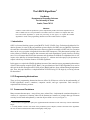
Abstract
LEAPS is a state-of-the-art production system compiler that produces the fastest sequential executables of OPS5 rule sets. The performance of LEAPS is due to its reliance on complex data structures and search algorithms to speed rule processing. In this paper, we explain the LEAPS
algorithms in terms of the programming abstractions of the P2 data structure compiler.
1 Introduction
OPS5 is a forward-chaining expert system [McD78, For81]. LEAPS (Lazy Evaluation Algorithm for Production Systems) is a state-of-the-art production system compiler for OPS5 rule sets [Mir90].2 Experimental results have shown that LEAPS produces the fastest sequential executables of OPS5 rule sets; execution
times can be over two orders of magnitude faster than OPS5 interpreters. This phenomenal speedup is due
to the reliance of LEAPS on complex data structures and search algorithms to greatly increase rule firing
rates. It is well-known that LEAPS data structures and algorithms are difficult to comprehend; this is due,
in part, to the inability of relational database concepts (i.e., relations and select-project-join operators) to
capture critical lazy-evaluation features of LEAPS algorithms.
In this paper, we explain the LEAPS algorithms in terms of the container-cursor programming abstractions
of the P2 data structure compiler [Sir93, Bat93]. Our specifications of the LEAPS algorithms were used as
the basis for the RL (Reengineered-LEAPS) project [Bat94] and have been validated through implementation. Thus, this paper describes a reimplementation of LEAPS using P2. We begin by reviewing relevant
P2 abstractions.
2 P2 Programming Abstractions
There are four programming abstractions that are offered by P2 that are critical to the understanding of
LEAPS algorithms: cursors, containers, composite cursors, and type expressions. Each concept is
explained in the following sections.
2.1 Cursors and Containers
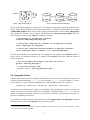
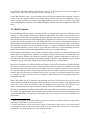
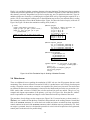
Many common data structures—arrays, binary trees, ordered lists—implement the container abstraction. A
container is a sequence of elements, where all the elements are instances of a single data type. Elements
can only be referenced and updated by a run-time object called a cursor (see Figure 1).
1. This research was supported in part by the Applied Research Laboratories at the University of Texas and Schlumberger.
2. Actually, OPS5c version 5 is the name of the production system compiler; LEAPS is the name of the algorithms.
We will use OPS5c/LEAPS and LEAPS interchangably in this paper.
1
A
container
cursor
a3
a1
elements
C
B
a2
b1
c1
c3
b2
b3
c2
c4
Figure 2. A Multicontainer Relationship
Figure 1. Basic P2 Abstractions
The P2 programming language is a superset of C. P2 introduces statements for cursor and container declarations, along with special operations on cursors and containers. An abbreviated declaration of a container
of EMPLOYEE_TYPE instances is shown below, along with declarations of a cursor (all_employees)
that references all elements of this container and another cursor (selected_employees) that references only those elements whose deptno field has the value 10:
// Declaration of the employee container.
container <EMPLOYEE_TYPE> employee;
// Cursor that references all elements in the employee container.
cursor <employee> all_employees;
// Cursor that references selected elements of employee container.
cursor <employee> where “$.deptno == 10” selected_employees;
P2 offers an (extensible) set of container and cursor operations. For example, the foreach construct is
used to iterate over qualified elements of a container. The foreach loop below prints the names of
selected employees:
// For each element whose deptno field has the value 10.
foreach( selected_employees )
{
// Print the employee name.
printf( “%s\n”, selected_employees.name );
}
2.2 Composite Cursors
Complex data structures consist of multiple containers whose elements are interconnected by pointers. A
relationship among containers C1, C2, ..., Cn is a set of n-tuples <e1, e2, …, en> where element ei is a member of container Ci. Figure 2 depicts a relationship for containers A, B, and C whose 3-tuples are:
{(a3,b1,c1), (a3,b1,c3), (a1,b2,c4), (a2,b3,c2), (a2,b3,c4)}
A composite cursor enumerates the n-tuples of a relationship. More specifically, a composite cursor k is an
n-tuple of cursors, one cursor per container of a relationship. A particular n-tuple <e1, e2, ..., en> of a relationship is encoded by having the ith cursor of k positioned on element ei. By advancing k, successive ntuples of a relationship are retrieved.
As an example, a composite cursor c that joins elements of the department and employee containers
that share the same value of the deptno field is specified in P2 as:3
3. Note that predicates in P2 are expressed by strings. Field F of the element referenced by a cursor is denoted “$.F”. A cursor
over container with alias x is denoted “$x”.
2
compcurs < d department, e employee > where “$d.deptno == $e.deptno” c;
d and e are aliases for container names. (As we will see in Section 3.2, aliases are useful for expressing the
joins of containers with themselves in an unambiguous way). The foreach loop below prints (employee
name, department name) pairs. Readers may recognize this loop as a natural join between department and employee containers:
foreach( c )
{ printf( “%s %s\n”, c.e.name, c.d.name );
}
Occasionally, it is useful to retrieve only n-tuples of a relationship that involve specific objects. Suppose
we are interested only in the 3-tuples of Figure 2 that involve element b3 of container B (i.e., tuples
(a2,b3,c2) and (a2,b3,c4)). Such a retrieval is called seeding a relationship with b3. Seedings are
expressed in P2 by augmenting the compcurs declaration with a given clause (which lists aliases of all
containers that are to be seeded). Prior to a foreach, the given cursors must be positioned on the seeding elements. The above example with b3 would be expressed by the following compcurs declaration
and foreach code fragment:
// Declare seeded_composite_cursor seeded by b.
compcurs < a A, b B, c C > given < b > seeded_composite_cursor;
// Position seeded_composite_cursor.b
position( seeded_composite_cursor.b, address_of(b3) );
// Iterate over seeded tuples.
foreach( seeded_composite_cursor )
{ ... }
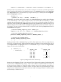
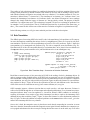
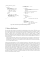
Updating elements within a foreach loop is possible. Such updates may affect the n-tuples that are
retrieved by a composite cursor. Again consider the example of composite cursor c which returns pairs of
related department and employee elements. The foreach of Figure 3a deletes the department
element for each retrieved ordered pair.
(a)
foreach ( c )
{ delete(c.d);
(b)
}
“blind” join
(
(
(
(
(
(
d1,
d1,
d1,
d2,
d2,
d3,
e1
e2
e3
e4
e5
e6
)
)
)
)
)
)
(c) “valid” join
( d1, e1 )
skip
( d2, e4 )
skip
( d3, e6 )
Figure 3. Updating elements within a foreach loop.
Suppose the code fragment of Figure 3a was executed. Figure 3b shows the sequence of tuples that would
be processed by the foreach loop during a “blind” retrieval. Blind or traditional database retrievals do
not take into account changes (e.g., deletions) made to elements since the last composite cursor advancement. What is actually needed is a “validated” retrieval of n-tuples, where tests are performed prior to each
composite cursor advancement to make sure that the next n-tuple is meaningful. Figure 3c shows the tuples
produced during a validated retrieval.
3
P2 supports validation of n-tuples using the valid clause of a composite cursor declaration. The following declaration and code fragment eliminates the problems of a blind retrieval of (department,
employee) tuples by returning tuples of undeleted elements:
compcurs < d department, e employee >
where “$d.deptno == $e.deptno”
valid “!deleted($d) && !deleted($e)” valid_composite_cursor;
foreach( valid_composite_cursor )
// Skips tuples with deleted elements.
{ delete( valid_composite_cursor.d );
}
Note that tuple validation is more general than merely testing for tuple deletion. P2 permits any predicate
to be used for element validation. For example, the deptno field of a department element might be
updated within a foreach loop. In this case, the department element has not been deleted, but its
modification may affect the sequence of (valid) tuples that can be produced. Tuple validation is a generalpurpose feature that is useful in graph traversal and garbage collection algorithms, where cursor validation
is needed to ensure correct executions.
2.3 Type Expressions
P2 programs are written in terms of cursor, composite cursor, and container abstractions without regard to
how these abstractions are implemented. The P2 compiler automatically translates P2 declarations and
operations into C code. In order for P2 to accomplish this, P2 users must specify an implementation of
these abstractions by composing building-blocks from the P2 library. Such a composition is declared in a
typex (type expression) declaration:
typex
{
simple_typex = top2ds[qualify[dlist[malloc[transient]]]];
}
simple_typex is a composition of five P2 components. Each component encapsulates a consistent data
and operation refinement of the cursor-container abstraction and is responsible for generating the code for
this refinement [Sir93]. The top2ds layer, for example, translates foreach statements into primitive
cursor operations (reset, advance, end_of_container); qualify translates qualified advance
operations into if tests and unqualified advance operations; dlist connects all elements of a container
onto a doubly-linked list; malloc allocates space for elements from a heap; and transient allocates
heap space from transient memory. P2 code generation relies on sophisticated macro expansion and partial
evaluation techniques [Bat93].
Altering a typex declaration yields a different implementation of cursors and containers. This powerful
feature greatly assists tuning and maintaining P2 programs, as typex declarations generally account for a
very small fraction of a P2 program.
3 The LEAPS Algorithms
As mentioned earlier, LEAPS produces the fastest executables of OPS5 rule sets, often outperforming
OPS5 interpreters that use RETE-match or TREAT-match algorithms by several orders of magnitude
[Bra91]. LEAPS translates OPS5 programs into C programs. Besides the expected performance gains
made by compilation, LEAPS relies on special algorithms and sophisticated data structures to make rule
processing efficient.
4
LEAPS Compiler
ops5
rule
set
RL
translator
P2
file
P2
Compiler
C
file
Figure 4. Relationship between LEAPS and P2
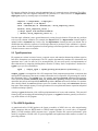
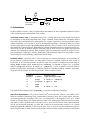
Figure 4 shows a relationship between the LEAPS compiler and P2. To reengineer LEAPS required us to
translate OPS5 rule sets into a P2 program; this translator was called RL (Reengineered Leaps). The RLgenerated P2 program would then be translated into a C program by the P2 compiler, thus effectively
accomplishing in two translation steps what the LEAPS compiler does in one. All of the LEAPS algorithms are embedded in the generated P2 program. In this section, we show that the LEAPS algorithms
have an elegant specification in P2. We assume that readers are familiar with the OPS5 language.
3.1 literalize Statements and OPS5 Terminology
OPS5 rule sets begin with “container” declarations called literalize statements:
(literalize guest name sex hobby)
The above statement declares a container guest whose elements have fields name, sex, and hobby.
LEAPS infers the data types of element fields; we chose to augment literalize statements by supplying
the data type for each field. Although this is a minor difference between LEAPS and RL, we note that the
next generation of LEAPS (called VENUS [Bro94]), like RL, uses explicit typing of fields.
An OPS5 rule set is a sequence of rules/productions of the form:
(p make_path
(context ^value make_path)
(seating ^id <id> ^pid <pid> ^path_done no)
(path ^id <pid> ^name <n1> ^seat <s>)
-(path ^id <id> ^name <n1>)
-->
(make path ^id <id> ^name <n1> ^seat <s>))
The name of the above production is make_path. Each of the clauses prior to the arrow --> are called
condition elements (CEs). The first three are positive; the last (with the minus sign) is negative. Positive
condition elements serve two purposes: 1) to express qualifications on containers and 2) to declare variable
bindings. For example, the first CE of the make_path rule qualifies elements from the context container
to those whose value field is ‘make_path’. The second CE qualifies elements from the seating container to those whose path_done field is ‘no’; in addition, it sets variable id to the value of the id field of
the qualified element and sets variable pid to the value of the pid field. The third CE qualifies elements
from the path container whose id field equals the value of the variable pid; in addition, variable n1 is
assigned the value of the name field and variable s is assigned the value of the seat field. In all, the positive CEs of this rule identify 3-tuples (context element, seating element, path element) that satisfy a
simple selection predicate.
Negated CEs are disqualification filters. The negated CE above disqualifies selected 3-tuples if there exists
a path element whose id field matches the value of variable id and whose name field matches the value
5
of variable n1 and whose seat field matches the value of s. In general, there can be any number of
negated CEs in a rule; however, there must at least one positive CE.
Clauses that follow the arrow --> are the actions of the rule. Once an n-tuple has been qualified, it fires the
actions of the rule. Actions of OPS5 rules include element creation, deletion, and modification; calls to
routines external to OPS5 are possible. In the make_path rule, the sole action is to insert a path tuple
whose id field equals variable id, whose name field equals variable n1, and whose seat field equals variable s.
3.2 LEAPS Overview
Forward-chaining inference engines, including LEAPS, use a match-select-action cycle. Rules that can be
matched (i.e., tuples found to satisfy their predicates) are determined; one n-tuple is selected and its corresponding rule is fired. This cycle continues until a fix point has been reached (i.e., no more rules can be
fired). RETE-match [For82] and TREAT-match [Mir91] algorithms are inherently slow, as they materialize
all tuples that satisfy the predicate of a rule. Materialized tuples are stored in data structures and have a
negative impact on performance as they must be updated as a result of executing rule actions. A fundamental contribution of LEAPS is the lazy evaluation of tuples; i.e., tuples are materialized only when needed.
This approach drastically reduces both the space and time complexity of forward-chaining inference
engines and provides LEAPS with its phenomenal increase in rule execution efficiency.
LEAPS assigns a timestamp to every element to indicate when the element was inserted or deleted. (For
reasons that we will explain later, elements are not updated. Instead, the old version is deleted and a new
version is inserted). Whenever an element is inserted or deleted, a handle to that element is placed on a
stack. In general, the stack maintains a timestamp ordering of elements, where the most recently updated
element is at the top of the stack and the least recently updated element is at the bottom.4
During a rule execution cycle, the top element of the stack is selected. This element is called the dominant
object (DO). The DO is used to seed the selection predicates of all rules. Rules are considered for seeding
in a particular order. Rules are sorted by their number of positive condition elements; the more positive
CEs, the sooner the rule will be seeded. Many rules have the same number of positive CEs; these rules are
seeded in order in which they were defined in the rule set. As soon as it is determined that the DO cannot
seed a n-tuple for a given rule, the next rule is examined.5 When all rules have been considered, the DO is
popped from the stack.
When a DO-seeded n-tuple is found, the corresponding rule is fired. The actions of the rule may invoke
element insertions, deletions, and updates, which in turn will cause more elements to be pushed onto the
stack. After a rule is fired, the selection of the next dominant object takes place. This execution cycle
repeats; execution terminates when a fix-point is reached. This occurs when the stack is empty.
Note that an element may be pushed onto the stack twice: once when it is inserted and a second time when
it is deleted. It is possible that a deleted element may be pushed onto the stack prior to the popping of its
inserted element. That is, the stack may contain zero, one, or two references to any given element at any
point in time.
4. There is an exception: an important LEAPS optimization violates the timestamp ordering. This optimization,
called shadow optimization, is discussed in Section 3.5.
5. Actually, DOs cannot be used to seed all rules in general. If a DO is from container C and C is not referenced in the
selection predicate of rule R, then the DO cannot seed R. Thus, the set of rules that a DO can seed can be pruned at
compile time to only those that actually reference the DO’s container.
6
The seeding of rule selection predicates by nondeleted elements has its obvious meaning. However, the
seeding of rule predicates by deleted elements is not intuitively obvious, and its meaning is closely associated with the semantics of negation. Associated with every container C is a shadow container S. Every element that is deleted from C is inserted in S. The timestamp of an element e in C indicates when e was
inserted; the timestamp of an element s in S indicates when s was deleted. Elements in S never undergo
changes; they simply define the legacy of elements in C that previously existed. The purpose of shadow
containers is to support time travel. The evaluation of negated CEs involves evaluating its predicate P on
its container C over a period of time. That is, LEAPS asks questions like: is predicate P true from time t0 to
time t1? The reason for this will become evident once the evaluation of negation is explained more fully.
In the following sections, we will give more technical precision to the above description.
3.3 Rule Translation
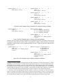
The difficult part of converting OPS5 rules into P2 code is the translation of rule predicates to P2 composite cursor declarations; translating the actions of rules is straightforward. There are six steps in rule predicate translation. The first is to convert qualifications of positive CEs to P2 predicates. Figure 5 shows the
correspondence of a nonnegated rule predicate (Fig. 5a) with a composite cursor declaration (Fig. 5b).
Note that each CE of the rule corresponds directly to a container that is to be joined. Also note that the use
of compcurs aliases permit containers to be joined with themselves in an unambiguous way.
(p rule14
(stage ^value labeling)
(junction ^type tee ^base_point <bp>
^p2 <p1> ^p2 <p2> ^p3 <p3>)
(edge ^p1 <bp> ^p2 <p1>)
(edge ^p1 <bp> ^p2 <p3> ^label nil)
-->
#define query14 “$a.value == ‘labeling’ &&
$b.type == ‘tee’ &&
$c.p1 == $b.base_point &&
$c.p2 == $b.p1 &&
$d.p1 == $b.base_point &&
$d.p2 == $b.p3 &&
$d.label == ‘nil’”
typedef compcurs < a stage, b cont_junction,
c cont_edge, d cont_edge >
where query14 curs14;
Figure 5a-b. Rule Translation Step 1: Conversion of Selection Predicates
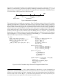
Recall that a central concept of rule processing in LEAPS is the seeding of rules by dominant objects. In
order to support seeding, multiple copies of an OPS5 rule are spawned, one copy of each different condition element that is being seeded. The second step in the rule translation process is to replicate a composite
cursor definition, one copy for each possible seed position. Figure 6a shows the format of a cursor declaration produced in Step 1; Figure 6b shows the replication of this rule with different seeds. Note that the
effect of this rewrite is to translate an n-way join to a more efficient (n-1)-way join.
OPS5 semantics imposes a fairness criterion that no n-tuple can fire a rule more than once. Fairness is
achieved in LEAPS through the use of timestamps and temporal qualifications. Every element has a timestamp that indicates when it was last updated (i.e., inserted or deleted). OPS5 semantics are realized by
requiring all elements of an n-tuple to have their timestamps less than or equal to the timestamp of the
dominant object that seeded the n-tuple.6 Figure 7a shows the format of a cursor declaration produced in
Step 2; Figure 7b shows the addition of temporal predicates to the where clause of the cursor. _ts is the
name of the timestamp field for every element.
Once a rule is fired, the composite cursor is placed on a stack, thereby suspending its execution. At some
later time, when the element that seeded the composite cursor again becomes dominant, the composite cursor is popped and advanced to the next n-tuple. During the time the cursor is on the stack, any or all of the
7
typedef compcurs < a .., b .., c .., d .. >
where query14 curs14;
typedef compcurs < a .., b .., c .., d .. >
given < a >
where query14 curs14_a;
typedef compcurs < a .., b .., c .., d .. >
given < b >
where query14 curs14_b;
typedef compcurs < a .., b .., c .., d .. >
given < c >
where query14 curs14_c;
typedef compcurs < a .., b .., c .., d
given < d >
where query14 curs14_d;
.. >
Figure 6a-b. Rule Translation Step 2: Replication of Composite Cursors by Seeding
typedef compcurs < a .., b .., c .., d .. >
given < a >
where query14 curs14_a;
#define temporal_query14
“$b._ts <= dominant_timestamp &&
$c._ts <= dominant_timestamp &&
$d._ts <= dominant_timestamp”
typedef compcurs < a .., b .., c .., d .. >
given < a >
where query14 “&&” temporal_query14
curs14_a;
Figure 7a-b. Rule Translation Step 3: Addition of Temporal Predicates
elements of the last n-tuple it produced could have been modified or deleted. Consequently, advancements
of composite cursors must be validated. This is accomplished by adding a valid predicate to each cursor
declaration. Figure 8a shows a cursor definition produced in Step 3; Figure 8b shows the addition of the
valid predicates.7
typedef compcurs < a .., b .., c .., d .. >
given < a >
where query1 “&&” temporal_query14
curs14_a;
#define valid_query “!is_deleted($a) &&
!is_deleted($b) &&
!is_deleted($c) &&
!is_deleted($d)”
typedef compcurs < a .., b .., c .., d .. >
given < a >
where query14 “&&” temporal_query14
valid valid_query14
curs14_a;
Figure 8a-b. Rule Translation Step 4: Addition of Validation Predicates
6. Things are actually a bit more complicated. In the case where a container C is being joined with itself, we want to
eliminate pairs of the same object (c,c) which could be generated more than once. To avoid such duplication, timestamp qualifications on containers “to the left” of the container of the seeding dominant object to have timestamps ≤
the timestamp of the DO and qualifications on containers “to the right” of the seeding container to be < the timestamp
of the DO [Bra93b]. The notion of “left” and “right” is determined by the order in which containers are listed to be
joined. Note that LEAPS did generate multiple tuples as it did not enforce the ideas outlined in this footnote.
7. Technically, cursors are not popped off the stack; pointers to cursors are overwritten. A stack item contains a
pointer to an element, the identifier of the container to which the element belongs, a pointer to a composite cursor
whose execution has been suspended, and an identifier of the rule to which the composite cursor belongs. When a cursor is popped, the cursor pointer is set to null. A stack item is popped only when all rules have been seeded.
8
Negated CEs are disqualification filters. The LEAPS interpretation of negation is depicted in Figure 9. An
element e is created at time t0 and seeds an n-tuple by advancing a composite cursor at times t1 ... t4. Let P
be the predicate of a negated CE and t be the time of a composite cursor advancement. LEAPS determines
if P is true at time t or at any time since e has been created.
time
t0
object e created
t2
t1
t3
t4
CC advanced
Figure 9. Interpretation of Negation
This interpretation has two significant consequences. First, LEAPS must maintain a history of all container
elements so that time can be “rolled back” to evaluate P. This is realized by creating a shadow container for
each container to be is a repository of the versions of elements that have since been modified or deleted.
Because shadow elements are tagged with the timestamp of their removal from the primary (nonshadow)
container, time travel is possible. Shadow containers are a major source of complexity in LEAPS. Second,
because predicate P may be valid at some time t does not mean that P is valid at later times. Consequently,
predicate P must be used to filter elements both in the where clause of a composite cursor and in the
valid clause as well. Figure 10a shows a rule with negation and Figure 10b shows one of its P2 composite
cursor counterparts (i.e., the one seeding in position a). Note that N5_4(..) is a boolean function (generated by RL) that expresses the filter of the negated CE.8
(p rule5
(stage ^value detect_junctions )
(edge ^p1 <bp> ^p2 <p2> ^joined false )
(edge ^p1 <bp> ^p2 <p3> ^p2 <> <p2>
^joined false )
-(edge ^p1 <bp> ^p2 <> <p2> ^p2 <> <p3> )
-->
#define query5
“$a.value == ’detect_junctions’ &&
$b.joined == ’false’ &&
$c.p1 == $b.p1 &&
$c.p2 != $b.p2 &&
$c.joined == ’false’ &&
N5_4(&$b,&$c)”
#define temporal_query5
“$a._ts <= dominant_timestamp &&
$b._ts <= dominant_timestamp &&
$c._ts <= dominant_timestamp”
#define valid_query5
“!is_deleted($a) &&
!is_deleted($b) &&
!is_deleted($c) &&
N5_4(&$b,&$c)”
typedef compcurs < a cont_stage, b cont_edge,
c cont_edge >
given < a >
where query5 && temporal_query5
valid valid_query5
curs5_a;
Figure 10a-b. Rule Translation Step 5: Placement of Negated Predicate Filters
8. Negated CE filters, like N5_4(..) have a simple realization in P2. The filter is (1) to test the container of the
negated CE for any element that satisfies predicate P of the negated CE, and (2) to examine the corresponding shadow
container if any element satisfies P and whose timestamp is greater than the dominant timestamp. If qualified elements are found in either container, N5_4(..) returns false. Both qualifications can be easily expressed using cursors with the obvious selection predicates over the container and shadow container.
9
Finally, it is possible for shadow container elements to become dominant. The idea here is that a container
element may block the qualification of n-tuples because it satisfied a negated CE filter. With the deletion of
this element, previously disqualified (or blocked) n-tuples may now be qualified (unblocked). Tests for
unblocked tuples are created by (a) modifying the original OPS5 rule by replicating the negated CE as a
positive CE, (b) converting the resulting rule via the translation steps we have just outlined, and (c) seeding
the resultant composite cursor with the shadow object. Figure 11a shows the result of step (a) to the rule of
Figure 10a; Figure 11b shows the translation resulting from (b) and (c).
(p rule5
(stage ^value detect_junctions )
(edge ^p1 <bp> ^p2 <p2> ^joined false )
(edge ^p1 <bp> ^p2 <p3> ^p2 <> <p2>
^joined false )
(edge ^p1 <bp> ^p2 <> <p2> ^p2 <> <p3> )
-(edge ^p1 <bp> ^p2 <> <p2> ^p2 <> <p3> )
-->
#define query5d
“$a.value == ’detect_junctions’ &&
$b.joined == ’false’ &&
$c.p1 == $b.p1 &&
$c.p2 != $b.p2 &&
$c.joined == ’false’ &&
$d.p1 == $b.p1 &&
$d.p2 != $b.p2 &&
$d.p2 != $c.p2 &&
N5_4(&$b,&$c)”
#define temporal_query5d
“$a._ts <= dominant_timestamp &&
$b._ts <= dominant_timestamp &&
$c._ts <= dominant_timestamp &&
$d._ts <= dominant_timestamp”
#define valid_query5d
“!is_deleted($a)
!is_deleted($b)
!is_deleted($c)
!is_deleted($d)
N5_4(&$b,&$c)”
&&
&&
&&
&&
typedef compcurs < a cont_stage, b cont_edge,
c cont_edge, d shadow_edge >
given < d >
where query5d && temporal_query5d
valid valid_query5d
curs5_d;
Figure 11a-b. Rule Translation Step 6: Seeding of Shadow Elements
3.4 Other Issues
There are additional issues regarding the translation of OPS5 rule sets into P2 programs that are worth
mentioning. First, when an element is inserted in LEAPS, it is pushed onto a wait-list stack for subsequent
seeding. Composite cursors, whose execution was suspended, are placed on a join-stack. The stack whose
top element has the most recent timestamp is chosen to be the dominant object on the next execution cycle.
In RL (and in other versions of LEAPS), the wait-list stack and join stack are unified. This gives a very
compact and elegant representation of the primary cycle loop (see Figure 12a). Note that the “unified”
stack is represented as a container, and top is a cursor that references the top element of the stack.
The procedures for rule firings are also compact (see Figure 12b). If a cursor has not yet been created (i.e.,
¬fresh), one is malloced from the heap, initialized, and positioned on the seeding element. Control then
falls to the foreach statement. If a cursor has been created (and whose execution has been suspended),
control continues at the end of the foreach statement (where validation tests are performed by P2). Once
an n-tuple is generated, the rule is fired and the procedure is exited. After all n-tuples have been generated,
control passes to the next rule for possible firing.
10
execute_production_system()
{
while(1) {
// Get the top of the stack.
reset_start(top);
if (end_of_container(top)) {
// The stack is empty.
// We’re at a fix-point.
break;
}
else {
// The stack is not empty.
fresh = !top.curs;
dom_timestamp = top.time_stamp;
(*top.current_rule)();
}
}
}
void seed_rule14_a ( void )
{ curs14_a *c;
if (fresh) {
c = (curs14_a*)malloc(sizeof(curs14_a));
top.curs = (void*) c;
initk(*c);
position(c->a,top.cursor_position);
} else {
c = (curs14_a *) top.curs;
goto cnt;
}
foreachk(*c) {
fire_rule14_a( c );
return;
cnt: ;
// perform valid tests here
}
}
free(c);
fresh = TRUE;
top.current_rule = nextrule;
nextrule(); // call seed_rule proc for
// next rule firing
Figure 12a-b. Execution Cycle and Rule Seeding Procedures
3.5 Notes on Data Structures
We stated earlier that elements are not updated, but rather deleted and then reinserted. While this seems
odd, it actually plays an integral role in the design of the LEAPS data structures for containers. The basic
idea is that composite cursors on the unified stack may point to elements that have been deleted. To
advance a composite cursor in such situations, elements can only be logically deleted (i.e., flagged
deleted); their storage space cannot be physically reclaimed. (Or more accurately, their storage space cannot be reclaimed until no cursor is referencing it). Hence the need for modeling updates as deletions followed by insertions.
LEAPS performed rudimentary garbage collection, where the physical space of elements is reclaimed. We noted
that maintaining reference counts (or whatever LEAPS actually does) adds considerable run-time overhead. For
the applications of LEAPS that we have seen, garbage collection at fix-point time offers a much faster and simpler
way to accomplish garbage collection.
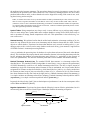
Another unusual requirement for a LEAPS container data structure is that elements must be stored in
descending timestamp order. One reason is to maintain OPS5 semantics. Another is to be consistent with
the general expert-system philosophy that the n-tuple that is selected for rule firing should have the most
recent timestamps. The simplest data structure that LEAPS could use as a container implementation is a
doubly-linked list, where deleted elements are still “connected” in that cursors on deleted elements can be
advanced to nondeleted elements. The figure below shows two cursors on a container (implemented by a
list). Cursor A points to an element with timestamp 8; cursor B points to a deleted element with timestamp
7). When cursor B is advanced, it will be positioned on the next undeleted element of the container whose
timestamp is less than 7. In general, it is possible that B may need to traverse a chain of deleted elements
before the first undeleted element is reached.
11
A
12
8
5
(deleted records
are shaded)
7
2
1
B
4 Optimizations
LEAPS (and RL) include a variety of optimizations than enhance the basic algorithms outlined in Section
3. We explain the major optimizations in this section.
Timestamp Ordered Lists. A timestamp ordered list is a doubly-linked list where (undeleted) elements
are maintained in descending timestamp order. Unlike “standard” doubly-linked lists, timestamp ordered
lists perform query modifications for optimizations. For example, a typical rule selection predicate requires
element timestamps to be less than or equal to the dominant timestamp. A timestamp ordered list would
use this requirement to optimize the reset_start operation, which positions a cursor on the first record
that satisfies the selection predicate. What happens is that the timestamp predicate is applied to the first elements of the list until an element qualifies. From that point on, there is no need for qualifying subsequent
elements due to timestamp ordering. Thus, predicates applied to subsequent elements do not involve temporal qualification. Other types of query optimizations with timestamp ordered lists are possible; readers
are encouraged to see the tlist[] component in the P2 library.
Predicate Indices. A predicate index is a list of elements of a container that satisfy a given predicate. (In
the AI literature, predicate indices are called alpha memories). Predicate indices are quite useful in
LEAPS/RL, as the selection predicates of rules are static. For example, to minimize the search time for
finding stage elements whose value field has “labeling” (in rule14 of Figures 5-8), a predicate
index for stage using predicate “$.value == ‘labeling’” is used. In general, a predicate index is
created for each positive (and negative) condition element of a rule that references constants. Again looking at rule14 as an example, the following predicate indices would be created:
Condition
Element #
Container
Predicate to index
(empty if no index created)
#1
stage
$.value == ‘labeling’
#2
junction
$.type == ‘tee’
#3
edge
#4
edge
$.label == ‘nil’
A predicate index component in P2, predindx[], is a minor modification of tlist[].
Active Rule Optimization. k-way joins can lead to O(nk) execution times, where n is the number of ele-
ments in a container. Eliminating costly searches that are known, a priori, not to yield n-tuples, often provides great performance advantages. The active rule optimization is the skipping of rules to be seeded
because it is known that the rule cannot generate n-tuples. This optimization requires the presence of predicate indices. When a predicate index is an empty list (i.e., there are no elements in the container that satisfy the given selection predicate), we know that a seeded rule cannot produce n-tuples. It is a simple
matter to augment the definition of the predicate index layer to accept as a further annotation two procedures. One procedure is called when the predicate index becomes empty; another procedure is called when
12
the predicate index becomes nonempty. The procedures themselves merely increment a counter for each
rule that uses the predicate index. If the counter for a rule is nonzero (meaning that there are one or more
predicate indices that are null), we know that the rule can be skipped for seeding. If the count is zero, seeding the rule may produce n-tuples.
In RL, we examine the counter for every rule that could be seeded by a dominant object. Thus, if there are n rules,
there are n tests. In general, the number of rules that are active at any one time is rather small. Thus, if the list
(container?) of active rules is maintained dynamically, performance of LEAPS should be enhanced. In particular,
we conjecture that as the number of rules per rule set increases, a scheme to maintain dynamically the list of rules
may offer significant performance advantages.
Symbol Tables. String comparisons are always costly. A more efficient way to perform string comparisons is to enter strings into a symbol table and to compare handles to strings. Since OPS5 allows only ==
and != operations on strings, handle comparisons work well. This optimization is also called string con-
stant enumeration.
Shadow Stacking. We explained earlier that the unified stack maintains a timestamp ordering of its ele-
ments; the top element has the most recent timestamp and the bottom element has the oldest. Deleted
objects are called shadows. Experience has shown that shadows rarely succeed in seeding rules (i.e., producing n-tuples to fire). As there can be many shadows on the stack at any given moment, a large fraction
of LEAPS run time is consumed processing shadows.
A way to minimize the processing time for shadows is to place them at bottom of the stack, rather than at
the top. This invalidates the property that the stack maintains elements in descending timestamp order, but
has the advantage that shadow processing becomes more efficient (i.e., particularly in the presence of
active rule optimizations). The increase in LEAPS performance can be dramatic with shadow stacking.
Hashed Timestamp Ordered Lists. The standard LEAPS data structure is a timestamp ordered list,
described above. The standard LEAPS join algorithm is nested loops. A way to improve the performance
of LEAPS dramatically would be to use hashed timestamp ordered lists. The idea is simple: instead of
maintaining a single list of timestamp ordered elements, b lists are maintained, one list per bucket. Bucket
assignments of elements are based on a hash key, which should also be a join key. As a result, search times
for elements on inner loops of joins are reduced by a factor of b (i.e., a fraction of (b-1)/b of the elements
have been eliminated as they don’t hash to the right join key). Hashed timestamp ordered lists (hlist[])
is a simple variation on timestamp ordered lists (tlist[]); hashed timestamp ordered predicate indices
(hpredindx[]) is a simple variation on predicate indices (predindx[]).
In general, the idea of using “hash” joins to obtain improved performance is an obvious consequence of the
work of Brant and Miranker [Bra93a].
Negation Optimization. Experience has shown that the following is not an effective optimization, but it is
an interesting idea never-the-less. Recall Figure 9 that helps illustrate the meaning of negation:
[t0,t1]
[t0,t2]
[t0,t3]
[t0,t4]
time
t0
object e created
t2
t1
CC advanced
13
t3
t4
A great deal of time is spent evaluating predicates of negated condition elements. In the case that a dominant object can seed multiple n-tuples (as in the above figure where object e seeds 4 n-tuples), it is possible
to optimize the processing of predicates of negated CEs. The idea is simple: when the negated CE is
applied to tuple at time t2, the truth value of its predicate must be determined for the interval [t0,t2]. Note
that the predicate must have been true for all previously tested intervals, e.g., [t0,t1], since had the predicate
failed, it would not be possible to seed further tuples. The optimization is to avoid replicate evaluation of a
negated predicate over the same interval. To test the validity of a predicate in interval [t0,t2], it is sufficient
to test the validity only over the interval [t1,t2], as the truth of the predicate in [t0,t1] has already been established.
As mentioned above, experience has shown that a dominant object typically seeds at most one n-tuple per
rule. Consequently, the conditions for the above optimization don’t seem to arise.
Malloc optimization. The Unix malloc optimization is very slow. LEAPS relied on its own memory allocation scheme. We tried to do something similar with a layer in P2 which performs the duties of malloc
on our own, home-grown memory allocation scheme. As it turns out, gnu malloc is more efficient, so we
did not pursue malloc optimization further.
5 RL Implementation
Of course, there are lots of details of LEAPS that are not explained in this paper. We recommend that the
interested readers examine the P2 files that are generated by RL. These files have embedded comments and
are fairly easy to understand with this paper.
When RL is run without command line arguments, the following options are shown:
Usage: rl [options] file
file.ops read; file.p2 is generated (see -s option)
Options:
-a active rule optimization
-c string constant enumeration optimization
-d debugging mode for op code generation
-e leaps debugging mode
-h shadow stacking optimization
-i inline insert and delete operations
-l standard leaps options (-achmp)
-m malloc optimization
-n negation optimization
-p predicate indexing included
-s print to standard output, not file.p2
-t include timestamp layer
-x add attribute indices
-1 no explicit shadow container
The -achlmnp options were discussed as optimizations in Section 4. The -de options are purely for
debugging RL. Options -x1 are not fully implemented. The -t option has not been fully tested, but
whether or not it is selected should make little or no difference in performance. (RL generates timestamps
to match those of LEAPS when -t is not selected; if -t is selected, a timestamp layer assigns timestamps).
14
Acknowledgments. I am grateful to the Applied Research Laboratories for supporting this research. I
thank Dan Miranker and Bernie Lafaso for their patience in explaining the LEAPS algorithms to me, and I
also thank Jeff Thomas for his invaluable help in designing and implementing composite cursors.
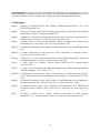
6 References
[Bat93]
D. Batory, V. Singhal, M. Sirkin, and J. Thomas, “Scalable Software Libraries”, Proc. ACM
SIGSOFT, December 1993.
[Bat94]
D. Batory, J. Thomas, and M. Sirkin, “Reengineering a Complex Application Using a Scalable
Data Structure Compiler”, submitted for publication.
[Big94]
T. Biggerstaff. “The Library Scaling Problem and the Limits of Concrete Component Reuse”,
IEEE International Conference on Software Reuse, November 1994.
[Bra91]
D. Brant, T.Grose, B. Lofaso, and D. Miranker, “Effects of Database Size on Rule System
Performance: Five Case Studies”, Proc. Very Large Databases, 1991.
[Bra93a]
D. Brant and D. Miranker, “Index Support for Rule Activiation”, Proc. ACM SIGMOD, May
1993.
[Bra93b]
D. Brant, “Inferencing on Large Data Sets”, Ph.D., Department of Computer Sciences,
University of Texas at Austin, 1993.
[Bro94]
J. Browne, et al. “A New Approach to Modularity in Rule-Based Programming”, Department
of Computer Sciences, University of Texas at Austin, April 1994.
[For81]
C. Forgy, OPS5 User’s Manual, Technical Report CMU-CS-81-135, Carnegie Mellon
University, 1981.
[For82]
C. Forgy, “A Fast Algorithm for the Many Pattern/Many Object Pattern Matching Problem”,
Artificial Intelligence, vol. 19 (1982), 17-37.
[McD78]
J. McDermott, A. Newall, and J. Moore, “The Efficiency of Certain Production Systems”,
Pattern Directed Inference Systems, Waterman, Hayes, Roth (ed), Academic Press, New York,
1978.
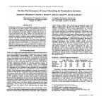
[Mir90]
D. Miranker, D. Brant, B. Lofaso, and D. Gadbois, “On the Performance of Lazy Matching in
Production Systems”, Proc. National Conference on Artificial Intelligence, 1990.
[Mir91]
D. Miranker and B. Lofaso, “The Organization and Performance of a TREAT-Based
Production System Compiler”, IEEE Transactions on Knowledge and Data Engineering,
1991.
[Sir93]
M. Sirkin, D. Batory, and V. Singhal, “Software Components in a Data Structure
Precompiler”, Proc. 15th International Conference on Software Engineering, May 1993.
15