Download JNM-ECA Series JNM-ECX Series JNM-ECS Series

INSTRUCTIONS
JNM-ECA Series
JNM-ECX Series
JNM-ECS Series
(Delta V4.3.6)
MEASUREMENT
USER’S MANUAL
For the proper use of the instrument, be sure to
read this instruction manual. Even after you
read it, please keep the manual on hand so that
you can consult it whenever necessary.
INMECA/ECX-USM-3a
AUG2007-08110237
Printed in Japan
JNM-ECA Series
JNM-ECX Series
JNM-ECS Series
(Delta V4.3.6)
MEASUREMENT
USER’S MANUAL
JNM-ECA Series
JNM-ECX Series
JNM-ECS Series
This manual explains how to adjust the system, how to set measurement
conditions, and other procedures for performing various measurements using the
ECA/ECX/ECS -NMR system.
Please be sure to read this instruction manual carefully,
and fully understand its contents prior to the operation
or maintenance for the proper use of the instrument.
NOTICE
• This instrument generates, uses, and can radiate the energy of radio frequency and, if not installed and used in
accordance with the instruction manual, may cause harmful interference to the environment, especially radio
communications.
• The following actions must be avoided without prior written permission from JEOL Ltd. or its subsidiary company
responsible for the subject (hereinafter referred to as "JEOL"): modifying the instrument; attaching products other than
those supplied by JEOL; repairing the instrument, components and parts that have failed, such as replacing pipes in the
cooling water system, without consulting your JEOL service office; and adjusting the specified parts that only field
service technicians employed or authorized by JEOL are allowed to adjust, such as bolts or regulators which need to be
tightened with appropriate torque. Doing any of the above might result in instrument failure and/or a serious accident. If
any such modification, attachment, replacement or adjustment is made, all the stipulated warranties and preventative
maintenances and/or services contracted by JEOL or its affiliated company or authorized representative will be void.
• Replacement parts for maintenance of the instrument functionality and performance are retained and available for seven
years from the date of installation. Thereafter, some of those parts may be available for a certain period of time, and in
this case, an extra service charge may be applied for servicing with those parts. Please contact your JEOL service office
for details before the period of retention has passed.
• In order to ensure safety in the use of this instrument, the customer is advised to attend to daily maintenance and
inspection. In addition, JEOL strongly recommends that the customer have the instrument thoroughly checked up by
field service technicians employed or authorized by JEOL, on the occasion of replacement of expendable parts, or at the
proper time and interval for preventative maintenance of the instrument. Please note that JEOL will not be held
responsible for any instrument failure and/or serious accident occurred with the instrument inappropriately controlled or
managed for the maintenance.
• After installation or delivery of the instrument, if the instrument is required for the relocation whether it is within the
facility, transportation, resale whether it is involved with the relocation, or disposition, please be sure to contact your
JEOL service office. If the instrument is disassembled, moved or transported without the supervision of the personnel
authorized by JEOL, JEOL will not be held responsible for any loss, damage, accident or problem with the instrument.
Operating the improperly installed instrument might cause accidents such as water leakage, fire, and electric shock.
• The information described in this manual, and the specifications and contents of the software described in this manual
are subject to change without prior notice due to the ongoing improvements made in the instrument.
• Every effort has been made to ensure that the contents of this instruction manual provide all necessary information on
the basic operation of the instrument and are correct. However, if you find any missing information or errors on the
information described in this manual, please advise it to your JEOL service office.
• In no event shall JEOL be liable for any direct, indirect, special, incidental or consequential damages, or any other
damages of any kind, including but not limited to loss of use, loss of profits, or loss of data arising out of or in any way
connected with the use of the information contained in this manual or the software described in this manual. Some
countries do not allow the exclusion or limitation of incidental or consequential damages, so the above may not apply to you.
• This manual and the software described in this manual are copyrighted, all rights reserved by JEOL and/or third-party
licensors. Except as stated herein, none of the materials may be copied, reproduced, distributed, republished, displayed,
posted or transmitted in any form or by any means, including, but not limited to, electronic, mechanical, photocopying,
recording, or otherwise, without the prior written permission of JEOL or the respective copyright owner.
• When this manual or the software described in this manual is furnished under a license agreement, it may only be used
or copied in accordance with the terms of such license agreement.
© Copyright 2002, 2003, 2004, 2007 JEOL Ltd.
• In some cases, this instrument, the software, and the instruction manual are controlled under the “Foreign Exchange and
Foreign Trade Control Law” of Japan in compliance with international security export control. If you intend to export
any of these items, please consult JEOL. Procedures are required to obtain the export license from Japan’s government.
TRADEMARK
• Windows is a trademark of Microsoft Corporation.
• All other company and product names are trademarks or registered trademarks of their respective companies.
MANUFACTURER
JEOL Ltd.
1-2, Musashino 3-chome, Akishima, Tokyo 196-8558 Japan
Telephone: 81-42-543-1111 Facsimile: 81-42-546-3353 URL: http://www.jeol.co.jp
Note: For servicing and inquiries, please contact your JEOL service office.
NOTATIONAL CONVENTIONS AND GLOSSARY
■ General notations
— CAUTION — :
?:
F:
Points where great care and attention is required when operating the
device to avoid damage to the device itself.
Additional points to be remembered regarding the operation.
A reference to another section, chapter or manual.
1, 2, 3 :
Numbers indicate a series of operations that achieve a task.
◆:
A diamond indicates a single operation that achieve a task.
File:
The names of menus, commands, or parameters displayed on the
screen are denoted with bold letters.
File–Exit :
A command to be executed from a pulldown menu is denoted by
linking the menu name and the command name with a dash (–).
For example, File–Exit means to execute the Exit command by selecting it from the File menu.
Ctrl :
Keys on the keyboard are denoted by enclosing their names in a
box.
■ Mouse operation
Mouse pointer:
An arrow-shaped mark displayed on the screen, which moves with
the movement of the mouse. It is used to specify a menu item,
command, parameter value, and other items. Its shape changes according to the situation.
Click:
To press and release the left mouse button.
Double-click:
To press and release the left mouse button twice quickly.
Drag:
To hold down the left mouse button while moving the mouse.
To drag an item, you point to an item on the screen and then drag it
using the mouse.
NMECA/ECX-USM-3
CONTENTS
1
FUNDAMENTALS OF DELTA
1.1 STARTING UP DELTA..........................................................................1-1
1.2 DELTA CONSOLE WINDOW............................................................1-2
1.2.1 The menu bar in the Delta Console window ..................................1-2
1.2.2 Tool Bar in the Delta Console Window .........................................1-4
2 SPECTROMETER CONTROL
2.1 SPECTROMETER CONTROL WINDOW.......................................2-1
2.1.1 Starting the Spectrometer Control Window .................................2-1
2.1.2 Connecting and Releasing Spectrometer.........................................2-2
2.1.3 Management of the Measurement Queue........................................2-7
2.1.4 Sample Monitor...............................................................................2-9
2.2 SAMPLE TOOL WINDOW ..............................................................2-10
2.2.1 Starting the Sample Tool Window ...............................................2-11
2.2.2 Display of SCM Related Information ...........................................2-12
2.2.3 Loading and Ejecting a Sample.....................................................2-13
2.2.4 Sample Spinning ...........................................................................2-16
2.2.5 Variable Temperature (VT)...........................................................2-17
2.2.6 Selecting the Deuterated Solvent ..................................................2-20
2.2.7 Control the NMR Lock .................................................................2-21
2.2.8 Shim Control .................................................................................2-23
2.3 EXPERIMENT EDITOR TOOL WINDOW ...................................2-27
2.3.1 Measurement File (Experiment File) ............................................2-28
2.3.2 Header Section ..............................................................................2-29
2.3.3 Instrument Section.........................................................................2-33
2.3.4 Acquisition Section .......................................................................2-35
2.3.5 Pulse Section .................................................................................2-37
2.4 AUTOMATION TOOL WINDOW...................................................2-39
2.4.1 Standard Mode in the Automation Window ................................2-39
2.4.2 Advanced Mode in the Automation Window ..............................2-42
2.5 RUN SAWTOOTH EXPERIMENT WINDOW ..............................2-47
2.6 VECTOR VIEWER WINDOW.........................................................2-48
2.6.1 Changing a Display .......................................................................2-49
2.6.2 Processing Menu ...........................................................................2-50
2.7 MAKE A NEW INSTANCE OF A SELECTED JOB COMMAND...2-51
2.8 90° PULSE WIDTH DISPLAY............................................................2-52
2.9 DISPLAYING AND CHANGE OF AN INSTRUMENT
PARAMETER ......................................................................................2-53
2.9.1 Display of an Instrument Parameter..............................................2-53
2.9.2 Changing an Instrument Parameter ...............................................2-54
2.10 SHAPE VIEWER.................................................................................2-55
2.10.1 How to Display a Shape ................................................................2-56
2.10.2 Calculation of Pulse Width and Attenuator Value ........................2-57
2.11 ABNORMAL DISPLAY OF A SPECTROMETER............................2-58
NMECA/ECX-USM-3
C-1
CONTENTS
2.12 VALIDATION ......................................................................................2-59
2.12.1 Executing Validation .....................................................................2-59
2.12.2 Printing Validation Result .............................................................2-60
2.12.3 Saving Validation Results to a File ...............................................2-60
2.13 DISPLAY OF LOG FILE .....................................................................2-61
2.13.1 Cryogen Log..................................................................................2-61
2.13.2 Machine Log..................................................................................2-62
2.13.3 Queue Log .....................................................................................2-63
2.14 PRE TUNE ...........................................................................................2-64
2.15 PROBE TUNE......................................................................................2-66
2.16 PROBE TOOL......................................................................................2-67
2.16.1 Display of Information for a Specified Nucleus............................2-67
2.16.2 Saving a Value to the Probe File ...................................................2-68
2.17 SHIM ON FID ......................................................................................2-69
2.18 GRADIENT SHIM TOOL ...................................................................2-71
2.18.1 Outline of the Gradient Shim.........................................................2-71
2.18.2 Gradient Shim Operation...............................................................2-73
2.19 SPECTROMETER CONFIGURATION ..............................................2-78
2.20 EXPERIMENT AND QUEUE MANAGMENT..................................2-80
2.20.1 Queue State....................................................................................2-80
2.20.2 Queue Menu ..................................................................................2-82
2.20.3 Restating Measurement (GO button).............................................2-83
2.20.4 Cancelling Measurement (STOP button) ......................................2-85
2.20.5 Measurement Priority ....................................................................2-86
2.20.6 Slot.................................................................................................2-86
2.20.7 Start Time of Measurement ...........................................................2-87
2.20.8 Measurement Information .............................................................2-87
2.21 APPENDIX...........................................................................................2-88
2.21.1 Probe Tuning..................................................................................2-88
2.21.2 Array Measurement .......................................................................2-95
3
ADJUSTMENT OF NMR PARAMETERS
3.1
3.2
3.3
3.4
3.5
3.6
3.7
4
PURPOSE OF MEASURING PULSE WIDTHS ..................................3-1
SPECTROMETER RF SYSTEM AND FACTORS AFFECTING
PULSE WIDTHS....................................................................................3-3
MEASUREMENT OF PULSE WIDTHS WHEN OUTPUT IS
USED AT HALF POWER......................................................................3-5
CALCULATION OF 90° PULSE WIDTHS AFTER THE
ATTENUATOR VALUE IS CHANGED ...............................................3-8
MEASUREMENT OF PULSE WIDTHS IN DEPT90 ..........................3-9
CALCULATION OF 90° PULSE WIDTH OF SELECTIVE
EXCITATION PULSES .......................................................................3-10
USAGE OF PULSE CALCULATOR TOOL ....................................3-12
USAGE OF PULSE SEQUENCES
4.1 EXTENSION SEQUENCES..................................................................4-3
4.1.1 dante_presat.....................................................................................4-3
4.1.2 Presaturation ....................................................................................4-4
4.1.3 Homo Decouple...............................................................................4-5
C-2
NMECA/ECX-USM-3
CONTENTS
4.1.4 noe ...................................................................................................4-6
4.1.5 decoupling .......................................................................................4-7
4.1.6 wet_suppression ..............................................................................4-8
4.1.7 raw_suppression..............................................................................4-9
4.2 1D MEASUREMENT..........................................................................4-10
4.2.1 single_pulse.ex2 ............................................................................4-10
4.2.2 single_pulse_dec.ex2.....................................................................4-11
4.2.3 single_pulse_shape.ex2 .................................................................4-12
4.2.4 single_pulse_shape_slp.ex2 ..........................................................4-13
4.2.5 single_pulse_wet.ex2 ....................................................................4-15
4.2.6 apt.ex2 ...........................................................................................4-16
4.2.7 dept.ex2 .........................................................................................4-18
4.2.8 wgh.ex2 .........................................................................................4-21
4.2.9 difference_noe_1d.ex2 ..................................................................4-23
4.2.10 noe_1d_dpfgse.ex2........................................................................4-25
4.2.11 roesy_1d_dpfgse.ex2.....................................................................4-27
4.2.12 tocsy_1d_dpfgse.ex2.....................................................................4-30
4.2.13 double_pulse.ex2...........................................................................4-32
4.2.14 double_pulse_dec.ex2 ...................................................................4-34
4.3 2D MEASUREMENT..........................................................................4-36
4.3.1 cosy_pfg.ex2 .................................................................................4-36
4.3.2 dqf_cosy_phase.ex2 ......................................................................4-38
4.3.3 hetcor.ex2 ......................................................................................4-40
4.3.4 coloc.ex2 .......................................................................................4-42
4.3.5 hmbc_pfg.ex2................................................................................4-44
4.3.6 hmqc_pfg.ex2................................................................................4-47
4.3.7 hsqc_dec_phase_pfgzz.ex2 ...........................................................4-50
4.3.8 hsqc_tocsy_dec_phase_pfgzz.ex2.................................................4-52
4.3.9 inadequate_2d_pfg.ex2 .................................................................4-54
4.3.10 noesy_phase_pfgzz.ex2.................................................................4-56
4.3.11 t_roesy_phase.ex2 .........................................................................4-58
4.3.12 tocsy_mlev1760_phase.ex2...........................................................4-60
5
MULTINUCLEAR NMR MEASUREMENT
5.1 OUTLINE OF MULTINUCLEAR NMR MEASUREMENT ...............5-1
5.1.1 About Multinuclear NMR ...............................................................5-1
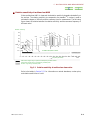
5.1.2 Relative Sensitivity of Multinuclear NMR......................................5-2
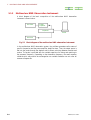
5.1.3 Multinuclear NMR Observation Instrument ...................................5-4
5.2 MULTINUCLEAR NMR MEASUREMENT........................................5-5
5.2.1 Multinuclear Observation Probes....................................................5-5
5.2.2 Operational Procedure for Multinuclear Measurement ...................5-6
5.2.3 Chemical Shifts and Reference Substances.....................................5-7
5.2.4 Observation of Nuclei Having a Resonance Frequency Close
to that of the 2H Nucleus .................................................................5-9
5.2.5 Sensitivity Enhancement by the Pulse Technique .........................5-10
5.3 SPECIAL PHENOMENA AND PRECAUTIONS FOR
MULTINUCLEAR NMR MEASUREMENT......................................5-11
5.3.1 Precautions for Sample Preparation ..............................................5-11
5.3.2 Selection of Sample Tubes ............................................................5-11
NMECA/ECX-USM-3
C-3
CONTENTS
5.3.3
5.3.4
5.3.5
5.3.6
5.3.7
Problems Involved with a Wide Chemical Shift Range ................5-12
Signal Fold-over ............................................................................5-13
Problems with Low Frequency Nuclei ..........................................5-14
Selecting 1H Decoupling................................................................5-14
Calculating the Pulse Width When There Is No Proper
Reference Sample ..........................................................................5-15
5.4 RELAXATION TIMES OF MULTINUCLEI ......................................5-16
5.4.1 General Tendencies of Relaxation Times of Multinuclei...............5-16
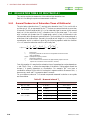
5.4.2 Reference Data for Relaxation Times and Measurement
Conditions of Principal Nuclei ......................................................5-17
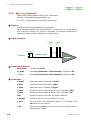
5.5 CHARTS AND MEASUREMENT MODES FOR
MULTINUCLEAR NMR MEASUREMENTS....................................5-19
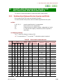
5.5.1 Relationships Between Nuclear Species and Sticks ......................5-19
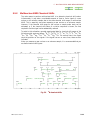
5.5.2 Multinuclear NMR Chemical Shifts..............................................5-23
INDEX
C-4
NMECA/ECX-USM-3
FUNDAMENTALS OF DELTA
Chapter 1 describes the operation of the fundamental processing tool of the Delta
program. The Delta program consists of various tools. Each tool uses two or more
windows. Processing, analysis, and plot out for NMR data are performed using these
tools.
1.1
1.2
STARTING UP DELTA...................................................................................... 1-1
DELTA CONSOLE WINDOW.......................................................................... 1-2
1.2.1 The menu bar in the Delta Console window .............................................. 1-2
1.2.2 Tool Bar in the Delta Console Window ..................................................... 1-4
NMECA/ECX-USM-3
1 FUNDAMENTALS OF DELTA
1.1
STARTING UP DELTA
This section assumes that operator is already logged into a workstation.
F Refer to the manual for the login procedure to a workstation.
■ When Delta icon is displayed on the desktop screen
u Double-click on the Delta icon.
The Delta program starts and the Delta Console appears.
Fig. 1.1 Delta Console window
NMECA/ECX-USM-3
1-1
1 FUNDAMENTALS OF DELTA
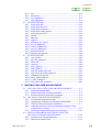
1.2
DELTA CONSOLE WINDOW
F
When you start the Delta program, the Delta Console window appears (
Fig. 1.2).
You can start all other tools from this window.
In the Delta Console window, you can start each Delta tool using the pull down menu
for each item of the menu bar, or the tool bar button. Move the mouse pointer to the pull
down menu or tool bar item, and click on the mouse left button.
Menu bar
Tool bar
View window
Fig. 1.2 Delta Console window
1.2.1
The menu bar in the Delta Console window
The list of items is displayed beneath of the title bar of the Delta Console window. This
is called the “menu bar”. Select any function in this menu bar using the mouse.
Fig. 1.3 Menu bar of the Delta Console window
■ Pull down menu
Each item of the menu bar has a “pull down menu”. When you select a menu bar item
Fig. 1.5).
using the mouse left button the pull down menu appears (
To select an item from the pull down menu, drag the mouse (with the left button of the
mouse depressed), and releasing the left button of the mouse over the item you want to
select.
If you select a pull down menu by mistake, after moving the mouse pointer away from
the pull down menu, release the left mouse button.
The tool bar functions frequently used also appear as icons under the menu bar.
F
1-2
NMECA/ECX-USM-3
1 FUNDAMENTALS OF DELTA
Pull down
menu of file
Fig. 1.4 Pull down menu
■ Accelerator key
An accelerator key is displayed to the right on the pull down menu. If you enter this key
from the keyboard, you can quickly open a window or select an option.
In displayed an accelerator key, the “^” sign indicates the Ctrl key. For example, in the
case of [^O], this means pressing the O key while pushing the Ctrl key.
Fig. 1.5 Accelerator key
NMECA/ECX-USM-3
1-3
1 FUNDAMENTALS OF DELTA
1.2.2
Tool Bar in the Delta Console Window
The icons located under the menu bar form the “tool bar”.
A picture of each function is displayed on each button. To select a button, move the
mouse pointer onto a button and click the mouse left button.
Almost all buttons have the same function as the corresponding menu bar items.
Fig. 1.6 Tool bar in the Delta Console window
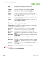
The following table explains the tool bar icon of the Delta Console window.
Icon
Button name
Explain
Data processor
This tool is for NMR data processing. If you specify a file name, a 1D
Processor or nD Processor window opens according to the number of
dimensions of data in the specified file.
Refer to the separate PROCESSING USER’S MANUAL for details
on the 1D Processor and nD Processor window.
F
Data slate
A data slate is a multipurpose NMR data display viewer. 1D, 2D, and
3D data can be displayed in a single window. Moreover, it can produce
a print of two or more spectra on the one chart.
For details, refer to the separate “PROCESSING USER’S MANUAL".
Data viewer
The data viewer is the tool provided for the display of multi-dimensional
NMR data. The contents of the window displayed change with the
numbers of dimensions of the data. This is used for obtaining both the
projection and the cross section of multi-dimensional NMR data.
File manager
This is a tool for saving and managing the directory that is used in the
Delta program and a file that is stored in the directory. If this tool is
used, not only can it easily reference a file in the directory, but it can
perform the copy, edit, deletion, change of name, and data conversion of
a file.
Presentation
manager
A presentation manager is a tool for customizing the plot format of NMR
data.
Parameter
viewer
A parameter viewer is a tool that displays information, such as a data set
parameter, report, sequence, processing history, and an electronic
signature.
Spreadsheet
A spreadsheet is a tool that displays information about a peak,
integration, and assignment in table format.
Connection
tool
A connection tool is to connect the display range of different data set.
Connection is performed using the reference of an axis. You can
associate any data sets regardless of the number of data points,
observation width, and magnetic field strength. If connection is
performed and the display range is changed to one data file, other related
data will be automatically set to the same display range.
Spectrometer
control tool
A spectrometer control tool is a tool which connects and disconnects the
host computer and the spectrometer.
Help
The help button displays an electronic manual using Acrobat ReaderⓇ.
F
1-4
NMECA/ECX-USM-3
SPECTROMETER CONTROL
2.1
SPECTROMETER CONTROL WINDOW............................................... 2-1
2.1.1
Starting the Spectrometer Control Window ........................................ 2-1
2.1.2
Connecting and Releasing Spectrometer............................................. 2-2
2.1.3
Management of the Measurement Queue............................................ 2-7
2.1.4
Sample Monitor................................................................................... 2-9
2.2
SAMPLE TOOL WINDOW .................................................................... 2-10
2.2.1
Starting the Sample Tool Window.................................................... 2-11
2.2.2
Display of SCM Related Information ............................................... 2-12
2.2.3
Loading and Ejecting a Sample......................................................... 2-13
2.2.4
Sample Spinning ............................................................................... 2-16
2.2.5
Variable Temperature (VT)............................................................... 2-17
2.2.6
Selecting the Deuterated Solvent ...................................................... 2-20
2.2.7
Control the NMR Lock ..................................................................... 2-21
2.2.8
Shim Control ..................................................................................... 2-23
2.3
EXPERIMENT EDITOR TOOL WINDOW........................................... 2-27
2.3.1
Measurement File (Experiment File) ................................................ 2-28
2.3.2
Header Section .................................................................................. 2-29
2.3.3
Instrument Section ............................................................................ 2-33
2.3.4
Acquisition Section ........................................................................... 2-35
2.3.5
Pulse Section ..................................................................................... 2-37
2.4
AUTOMATION TOOL WINDOW ......................................................... 2-39
2.4.1
Standard Mode in the Automation Window ..................................... 2-39
2.4.2
Advanced Mode in the Automation Window ................................... 2-42
2.5
RUN SAWTOOTH EXPERIMENT WINDOW...................................... 2-47
2.6
VECTOR VIEWER WINDOW ............................................................... 2-48
2.6.1
Changing a Display ........................................................................... 2-49
2.6.2
Processing Menu ............................................................................... 2-50
2.7
MAKE A NEW INSTANCE OF A SELECTED JOB COMMAND....... 2-51
2.8
90° PULSE WIDTH DISPLAY ............................................................... 2-52
NMECA/ECX-USM-3
2.9
DISPLAYING AND CHANGE OF AN INSTRUMENT PARAMETER2-53
2.9.1
Display of an Instrument Parameter ..................................................2-53
2.9.2
Changing an Instrument Parameter ...................................................2-54
2.10 SHAPE VIEWER .....................................................................................2-55
2.10.1 How to Display a Shape ....................................................................2-56
2.10.2 Calculation of Pulse Width and Attenuator Value ............................2-57
2.11 ABNORMAL DISPLAY OF A SPECTROMETER ................................2-58
2.12 VALIDATION ..........................................................................................2-59
2.12.1 Executing Validation.........................................................................2-59
2.12.2 Printing Validation Result .................................................................2-60
2.12.3 Saving Validation Results to a File ...................................................2-60
2.13 DISPLAY OF LOG FILE .........................................................................2-61
2.13.1 Cryogen Log......................................................................................2-61
2.13.2 Machine Log......................................................................................2-62
2.13.3 Queue Log .........................................................................................2-63
2.14 PRE TUNE ...............................................................................................2-64
2.15 PROBE TUNE..........................................................................................2-66
2.16 PROBE TOOL..........................................................................................2-67
2.16.1 Display of Information for a Specified Nucleus................................2-67
2.16.2 Saving a Value to the Probe File .......................................................2-68
2.17 SHIM ON FID ..........................................................................................2-69
2.18 GRADIENT SHIM TOOL .......................................................................2-71
2.18.1 Outline of the Gradient Shim ............................................................2-71
2.18.2 Gradient Shim Operation...................................................................2-73
2.19 SPECTROMETER CONFIGURATION..................................................2-78
2.20 EXPERIMENT AND QUEUE MANAGMENT......................................2-80
2.20.1 Queue State........................................................................................2-80
2.20.2 Queue Menu ......................................................................................2-82
2.20.3 Restating Measurement (GO button).................................................2-83
2.20.4 Cancelling Measurement (STOP button) ..........................................2-85
2.20.5 Measurement Priority ........................................................................2-86
2.20.6 Slot.....................................................................................................2-86
2.20.7 Start Time of Measurement ...............................................................2-87
2.20.8 Measurement Information .................................................................2-87
2.21 APPENDIX ..............................................................................................2-88
2.21.1 Probe Tuning......................................................................................2-88
2.21.2 Array Measurement ...........................................................................2-95
NMECA/ECX-USM-3
2 SPECTROMETER CONTROL
2.1
SPECTROMETER CONTROL WINDOW
The Spectrometer Control window controls spectrometer connection and NMR
measurement.
2.1.1
Starting the Spectrometer Control Window
Starts the Spectrometer Control window from the Delta Console window.
u Click on the
button in the Delta Console window.
The Spectrometer Control window opens.
? If you select Acquisition–Connect in the menu bar, the Spectrometer Control
window can also be started.
? In the Delta Console window, if you press the
C key while pushing the Ctrl key,
the Spectrometer Control window can start.
Fig. 2.1 Spectrometer Control window.
The Spectrometer Control window can control spectrometer function.
NMECA/ECX-USM-3
2-1
2 SPECTROMETER CONTROL
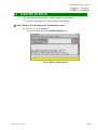
2.1.2
Connecting and Releasing Spectrometer
The connectable spectrometers are listed in the Spectrometer Control window.
By connecting with the spectrometer in this list, you can perform NMR measurement.
■ Connecting to spectrometer
There are three ways to connect to the spectrometer.
When performing out NMR measurement, connect in the Connect mode.
? Connection is restricted by the account logged into.
Refer to the "ADMINISTRATOR’S MANUAL" for these setting.
? Even if you have the right to connect, connection in a specified mode may not be
performed according to the state of the spectrometer.
Mode
Explanation
Monitor
Monitors the state and measurement conditions of the spectrometer. When other
users have already connected with spectrometer, only Monitor mode may be
connected. NMR measurement cannot be performed. However, measurement can
be reserved. Measurement can be started when anyone who has connected in
Connect mode releases the spectrometer.
Connect
NMR measurement and spectrometer control are performed in this mode.
Console
In this mode, deleting the jobs records to the Queue from other work stations,
forced release of spectrometer connection from other work stations, change in a job
priority, and rewriting of system files can be performed. However, NMR
measurement cannot be performed.
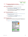
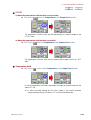
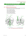
1. Select the target spectrometer using the mouse from the spectrometer list
displayed in the Spectrometer Control window and can be communicated.
Selection highlights the name of the selected spectrometer.
Selected spectrometer
Spectrometer list can
be communicated
2-2
NMECA/ECX-USM-3
2 SPECTROMETER CONTROL
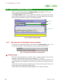
2. Click on the Connect button.
Node name of connection
mode and connection
place appear.
? If status display of the selected spectrometer is not Free, it cannot be connected in
the Connect mode. It is connected automatically in Monitor mode.
NMECA/ECX-USM-3
2-3
2 SPECTROMETER CONTROL
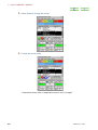
■ Release of a spectrometer
u Click on the Unlink button of the Spectrometer Control window.
Connection with a spectrometer is released and a connectable spectrometer is
displayed.
2-4
NMECA/ECX-USM-3
2 SPECTROMETER CONTROL
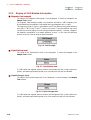
■ Confirming spectrometer information
The information on a spectrometer to connect or on the connected spectrometer can be
verified using the following procedures.
l Information of a spectrometer to connect
1. Select the spectrometer to connect in the Spectrometer Control window
using the mouse.
The name of the selected spectrometer is highlighted.
2. Click on the Info button.
The Info window opens.
Fig. 2.2 Info window (before connection)
? The kind of spectrometer, magnetic field strength, information appearing in
machine.info for this spectrometer, and its probe information are displayed.
l Information of on the connected spectrometer
u Click on the Info button in the Spectrometer Control window.
The Info window opens.
Fig. 2.3 Info window (after connection)
? In addition to the information before connection, user information and information on the connected workstation is displayed.
NMECA/ECX-USM-3
2-5
2 SPECTROMETER CONTROL
■ Display of the available spectrometer
u Click on the Free button in the Spectrometer Control window.
The node name and user for all available spectrometers on a network are investigated and displayed.
Connection is also canceled at this time.
2-6
NMECA/ECX-USM-3
2 SPECTROMETER CONTROL
2.1.3
Management of the Measurement Queue
In the Spectrometer Control window, the Queue measurement can be managed.
■ Starting measurement Queue
This is the starting method for the measurement Queue in the hold state.
u Click on the Go button in the Spectrometer Control window.
Measurement Queue starts in the Hold state.
? In normal measurement, if you click on the Submit button in the Experiment Tool
window, since the measurement Queue starts automatically, it is not necessary to
start the measurement Queue by the Go button.
■ Canceling measurement Queue
This is the canceling method of measurement Queue.
1. Select the measurement queue to cancel from the measurement Queue list
box displayed by the mouse.
The selected measurement Queue is highlighted.
2. Click on the STOP button in the Spectrometer Control window.
The selected measurement Queue is canceled.
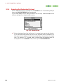
■ Changing Queue priority
Changing the priority value attached to each Queue can change the Queuing order. The
priority value is 0 to 255. Higher priority carries a greater value. The default priority is
32.
1. Change the connection mode to Console mode.
NMECA/ECX-USM-3
2-7
2 SPECTROMETER CONTROL
2. Select Queue to change the priority.
3. Change the priority value.
Measurement Queue order is changed when priority value is changed.
2-8
NMECA/ECX-USM-3
2 SPECTROMETER CONTROL
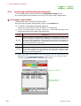
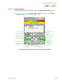
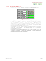
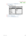
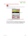
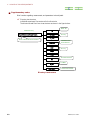
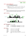
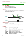
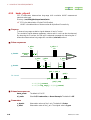
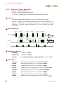
2.1.4
Sample Monitor
The state of the present sample can be displayed in the Spectrometer Control window.
u In the menu bar of the Spectrometer Control window, select Options—
Monitor Params, and turn ON the toggle switch.
Spinning speed of
spinner
Spinner status
Slot number of ASC
Status of
Temperature Control
Current state of the
sample
Sample Temperature
State of NMR lock
State of shim
Estimated time
of Measurement
completion
Lockロック信号の強度
signal Intensity
Remaining number
of repetitions
Remaining number
of accumulations
Liquid helium Level
Receiver gain
Liquid nitrogen level
Fig. 2.4 Sample monitor in the Spectrometer Control window
NMECA/ECX-USM-3
2-9
2 SPECTROMETER CONTROL
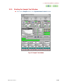
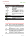
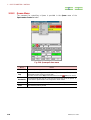
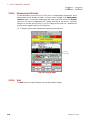
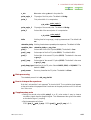
2.2
SAMPLE TOOL WINDOW
In the Sample Tool window, loading a sample, spinning, NMR lock, and shim
adjustment can be performed.
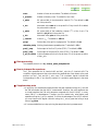
The main information displayed in the Sample Tool window is as follows：
Items
2-10
Explanation
Field Strength
Magnetic-field-strength [T] (Display only)
Helium
Liquid helium level [%] (Display only)
Nitrogen
Liquid nitrogen level [%] (Display only)
Sample State
Sample state (Load/Eject)
Spinner
Sample Spinning state (Spin/No spin) and spinning speed [Hz]
Temperature
Variable temperature state（ON/OFF）
Solvent
Deuterated solvent name
Lock Control
NMR lock condition (Gain/Level/Phase/Offset)
Shim Control
Lock signal intensity (display only) and shim conditions
NMECA/ECX-USM-3
2 SPECTROMETER CONTROL
2.2.1
Starting the Sample Tool Window
u Click on the Sample button in the Spectrometer Control window.
Fig. 2.5 Sample Tool window
NMECA/ECX-USM-3
2-11
2 SPECTROMETER CONTROL
2.2.2
Display of SCM Related Information
■ Magnetic field strength
The value of this magnetic field strength is only displayed. It cannot be changed in the
Sample Tool window.
The magnetic field strength provides very important information. NMR frequency can
be calculated from the magnetic field strength and a gyromagnetic ratio (γratio).
The frequency offset of 0 ppm is calculated so that it may become the precise reference
point (this is TMS for the 1H and 13C nuclei) of the scale. Using this method, any nuclei
can perform criterion setting of an axis using an absolute frequency. However, change of
the magnetic susceptibility of a sample produces an error. In this case, the reference
position of an axis is set up using an internal standard.
Fig. 2.6 Field Strength
■ Liquid-helium level
The value of this liquid-helium level is only displayed. It cannot be changed in the
Sample Tool window.
Fig. 2.7 Liquid-helium level
If it falls below the required amount, cautions (the background color of the screen turns
yellow), and warnings (the background color of screen turns red) will be indicated.
■ Liquid-nitrogen level
The value of this liquid-nitrogen level is only displayed. It cannot change in the Sample
Tool window.
Fig. 2.8 Liquid-nitrogen level
If it falls below the required amount, cautions (the background color of the screen turns
yellow), and warnings (the background color of the screen turns red) will be indicated.
2-12
NMECA/ECX-USM-3
2 SPECTROMETER CONTROL
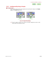
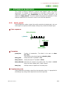
2.2.3
Loading and Ejecting a Sample
■ Sample state
The Load/Eject state of the present sample can be confirmed in display of the Sample
State in the Sample Tool window.
Loaded state
Ejected state
Fig. 2.9 Sample State display
? When the greener indicator turns yellow, this means changing from eject to load
state or eject from load state is shown.
NMECA/ECX-USM-3
2-13
2 SPECTROMETER CONTROL
■ Loading a sample
l When using the auto sample changer
When using the auto sample changer, a series of steps from changing to loading a sample
can be performed simply by automatically setting a slot number.
u Enter the slot number to set a sample on the auto sample changer in a Slot
in the Sample State of the Sample Tool window.
ｘ
After carrying the sample in the slot that specified on the auto sample changer, on
SCM, it is loaded and the sample state changes to load state.
? In order to prevent trouble during loading and ejecting a sample by the auto sample
changer, set Spectrometer Load/Eject Disable in the System tab of the Preferences Tool window to TRUE. The load and eject button of a sample are dimmed in
this way, and to prevent mistake in operation.
l When not using the auto sample changer
u Click on the
button in the Sample State of the Sample Tool window.
A sample is loaded, and the sample state changes into the load state.
2-14
NMECA/ECX-USM-3
2 SPECTROMETER CONTROL
■ Ejecting a sample
l When using the auto sample changer
When using the auto sample changer, a series of work from ejecting to changing the
sample can be performed simply setting a slot number.
u Enter the slot number 0 in the Slot in the Sample State of the Sample Tool
window.
The sample is ejected and carried on an auto sample changer. The sample state
changes to eject state.
? In order to prevent the trouble at the time of loading and ejection by the auto sample
changer, set Spectrometer Load/Eject Disable in the System tab of the Preferences Tool window to TRUE. The load and eject button of a sample are dimmed
by this operation, and this can prevent mistake in operation.
l When not using an auto sample changer
u Click on the
button in Sample State of the Sample Tool window.
A sample is ejected, and the sample state changes into the eject state.
NMECA/ECX-USM-3
2-15
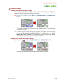
2 SPECTROMETER CONTROL
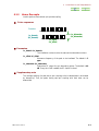
2.2.4
Sample Spinning
■ Spinning state
Load/eject state of the present sample can be verified in the display of a Sample State in
the Sample Tool window.
Spinning OFF
Spinning ON
Present spinning
speed
Target spinning
speed
Fig. 2.10 Spinner display
? When the green indicator turns yellow, this means changing from the spin-off state
to the spin on state or the spin-off state from the spin on state.
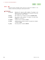
■ Spinner on
u Click on the
button in the Spinner of the Sample Tool window.
A sample begins a spinning and the sample state changes into the spin on state.
■ Spinner off
u Click on the
button in the Spinner of the Sample Tool window.
A sample is ejected, and the sample state changes into the eject state.
2-16
NMECA/ECX-USM-3
2 SPECTROMETER CONTROL
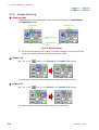
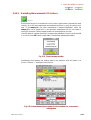
2.2.5
Variable Temperature (VT)
■ Sample temperature
The temperature control state of the sample can be verified by Temperature display in
the Sample Tool window.
l When the Temperature Hold function is not provided
VT ON
VT OFF
Present sample
temperature
Target sample
temperature
Fig. 2.11 Temperature display (without the Temperature Hold function)
? When the green indicator turns yellow, this indicates to change from VT OFF state
to VT ON state or VT OFF state from VT ON state is shown.
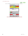
l When the Temperature hold function is provided
In order to use temperature hold function, after changing the value of TEMP_HOLD
_AVAILABLE in the machine.config file of the spectrometer into TRUE, it is
necessary to restart the spectrometer.
?
VT ON
VT OFF
Present sample temperature
Holding temperature
Target temperature
Fig. 2.12 Temperature display (with the Temperature Hold functional )
? When the green indicator turns yellow, this shows to change from the present VT
OFF state to VT ON state or VT OFF state from VT ON state.
? The temperature in a temperature hold is the temperature of the sample space (this
means holding this temperature during a sample exchange).
NMECA/ECX-USM-3
2-17
2 SPECTROMETER CONTROL
■ VT ON
l When the temperature hold function is not provided
u Click on the
button under Temperature in the Sample Tool window.
The temperature controller begins operation, and the state display of a sample
changes to the VT ON state.
? When
setting the temperature-exceeding boiling point and melting point of the
selected solvent to Target, a warning display appears, and the temperature setting is
reset.
l When the temperature hold function is provided
u Click on the button under Temperature in the Sample Tool window.
The temperature controller begins operation, and the state display of a sample
changes into the VT ON state.
? When setting the temperature exceeding boiling point and melting point of the
selected solvent to Target, a warning display appears, and the temperature setting is
reset.
2-18
NMECA/ECX-USM-3
2 SPECTROMETER CONTROL
■ VT OFF
l When the temperature hold function is not provided
u Click on the
button in Temperature of the Sample Tool window.
The temperature controller stops, and the state display of a sample changes to the
VT OFF state.
l When the temperature hold function is provided.
u Click on the
button in Temperature of the Sample Tool window.
The temperature controller stops, and the sample state changes into the VT OFF
state.
■ Temperature Hold
u Click on the
button under Temperature in the Sample Tool window.
In this the temperature hold mode, and sample exchange can be performed with the
state of VT ON.
? In order to prevent damage by fire from a heater, if you cannot terminate
sample exchange during a fixed time, VT is turned off automatically.
NMECA/ECX-USM-3
2-19
2 SPECTROMETER CONTROL
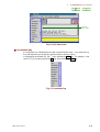
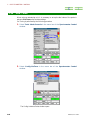
2.2.6
Selecting the Deuterated Solvent
Select a deuterated solvent of a sample from the Solvent list box. The following example
shows that CHLOROFORM-D has been selected.
If you make mistake in this setting, the NMR lock not only cannot be applied, but
reference setting will not be performed correctly.
Fig. 2.13 Solvent list box
? When selecting an item from the list box, it is convenient to use the skip function.
If you move the mouse pointer into the list box, and enter the first character of an
item name from the keyboard, it will skip automatically to the position of the target
item. For example, if C (a capital letter) is entered from the keyboard when the
mouse pointer is in the Solvent list box, it will skip to CHLOROFORM-D.
2-20
NMECA/ECX-USM-3
2 SPECTROMETER CONTROL
2.2.7
Control the NMR Lock
The NMR lock is controlled in the Lock Control part of the Sample Tool window.
Fig. 2.14 Lock Control
In the NMR lock a system, in order to retain the magnetic field stability, the magnetic
field is locked using NMR signal of 2H nucleus in the sample. If the magnetic field is
changed or drifts, the magnetic field will be stabilized using the Z0 axis shim coil.
Moreover, the lock signal intensity is used for shim adjustment. The intensity of a signal
becomes strong so that the magnetic field is uniform.
When using the NMR lock system, the 2H nucleus must be contained in the sample.
Usually, the 2H nucleus exists in the deuterated solvent, such as Chloroform-d,
Benzene-d6, and Acetone-d6.
Measurement is performed without applying the NMR lock for the sample in which the
2
H nucleus is not contained. Moreover, when measuring the 2H nucleus, measurement is
performed using the mode without the NMR lock.
NMECA/ECX-USM-3
2-21
2 SPECTROMETER CONTROL
■ NMR Lock Control Button
Click the following button in Lock Control to control the NMR lock.
Icon
Function
Explanation
Lock ON
The NMR lock is turned on to the 2H signal included in
sample. Wide range search of a lock signal is not performed.
Therefore, it is necessary to adjust Z0 in the Sawtooth
window so that a lock signal may adjust in advance to the
position of lock frequency.
Lock OFF
NMR lock is turned off.
However, since the output of the lock oscillator does not stop,
in addition to Lock OFF instruction, it is necessary to change
an instrument parameter LOCK OSC STATE to 2H OSC
OFF when observing a 2H nucleus.
Refer to the Parameter Tool for changing instrument
parameters.
Auto Lock
Wide range search of the lock signal is carried out, and if a
signal is found, the NMR lock will be turned on. Moreover,
the level and gain of the NMR lock will be adjusted
automatically.
Auto Lock&Shim
The Z1 axis and Z2 axis shim is adjusted automatically after
automatical locking.
Gradient Shim
Shimming is performed by gradient shim.
The execution conditions of the gradient shim are described
in gradient_solvent2 file of the instrument directory.
Gradient Shim&Lock
Automatically locking is performed after performing the
gradient shimming.
Optimize Lock
Phase
The lock signal phase is optimized. In order to use this
function, it is necessary to turn on the NMR lock in advance.
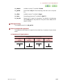
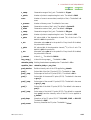
■ NMR lock relation parameter
2-22
Parameter
Explanation
ＮＭＲ lock state
(only display)
The NMR lock state at present is displayed.
Red is lock-off, yellow is during the search for the lock signal, and green is
lock-on.
Gain
This is a gain of the lock receiver. The amplification rate of a lock signal is
adjusted. Usually, the value described in the solvent.def file is set up. In
case of an auto lock, a gain is adjusted automatically and NMR lock signal
is detected.
Level
This is the output level of the lock channel. Usually, the value described in
the solvent.def file is set up. In case of an auto lock, the level is adjusted
automatically and an NMR lock signal is detected.
Phase
This is the lock signal phase. The value described in the shim file is set up.
A lock phase depends on RF filter in the mainly used probe and the lock
channel. Moreover, if the dielectric constant of a sample and an ion
concentration changes greatly, the lock phase may change.
Offset
This is the offset lock frequency. Usually, the value described in the
solvent.def file is set up. It is the frequency offset required in order to set
TMS as to 0 ppm.
NMECA/ECX-USM-3
2 SPECTROMETER CONTROL
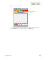
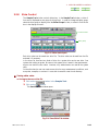
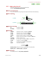
2.2.8
Shim Control
The Sample Tool window controls shimming. In the Sample Tool window, a shim of
four axes is displayed as one group (a shim group). In order to change a display group,
select the shim group to display from the Shim Groups list box, or select it from the list
box in the display shim axis.
Lock level meter
Shim group
Fig. 2.15 Shim control part
Each shim value can be saved as a shim file. The shim value can be read from the file
and used it if necessary.
In the shim file, there are two kinds of shim for a system shim and a user shim. One
system shim exists per probe. Moreover, this system shim is saved in the spectrometer ;
anyone can read this shim value. However, only administrator can rewrite the system
shim.
On the other hand, a user can create a user shim for every measurement conditions, such
as a probe, a sample, or a solvent. A user shim is saved to a user's local directory.
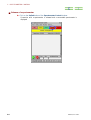
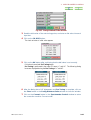
■ Saving shim value
l Saving to the user shim file
1. Click on the
button in the Sample Tool.
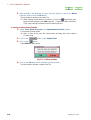
2. Click on the
button.
The Save Shim File window opens.
Fig. 2.16 Save Shim File window
NMECA/ECX-USM-3
2-23
2 SPECTROMETER CONTROL
3. After moving to the directory to save, input file name to save to the Name
input box, and click on the Ok button.
The shim value is saved to a user shim file.
button after speciWhen creating a new directory to save to, click on the
fying a directory name to the Path input box. Create and transfer a directory.
Then, input a saving file name into the file name input box.
?
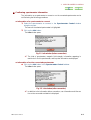
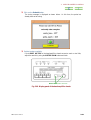
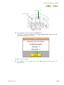
l Saving to the system shim file
1. Select Tools—Mode—Console in the Spectrometer Control window.
This becomes Console mode.
? Work is done by the user with administrator privilege, who user’s right to
Console mode.
2. Click on the
button in the Sample Tool.
3. Click on the
button.
The Confirm window opens.
Fig. 2.17 Confirm window
4. Click on the Ok button when saving a system shim file.
The shim value is saved to a system shim file.
2-24
NMECA/ECX-USM-3
2 SPECTROMETER CONTROL
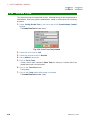
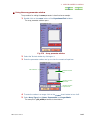
■ Reading a shim file
l Reading a system shim file
1. Click on the
button in the Sample Tool.
2. Click on the
button.
The Confirm window opens.
Fig. 2.18 Confirm window
3. Click on the Ok button when reading a system shim file.
A system shim is loaded.
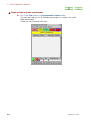
l Reading a user shim file
1. Click on the
button in the Sample Tool.
2. Click on the
button.
The Open Shim File window opens.
Fig. 2.19 Open Shim File window
3. Select a shim file name to read with the mouse, and click on the Ok button.
The shim file is read and the shim value is set to each axis. Information of the read
shim file appears on the Inform window.
Fig. 2.20 Inform window
NMECA/ECX-USM-3
2-25
2 SPECTROMETER CONTROL
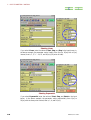
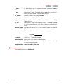
■ Shim control button and list box
The followings button and list box are used for controlling shims.
Button
Explanation
The spectrometer is always monitoring shim value and lock signal
intensity, It has memorized the best shim value at maximum lock signal
intensity. This best shim value is cleared.
The best shim value is called and the value is set to each axis.
The shim value displayed on the Shim Control part in Sample Tool is
updated to the shim value set to the spectrometer now.
Automatic shim adjustment of the specified axis is performed. When
performing automatic shim adjustment, select the combination of an axes to
perform automatic shim adjustment from the list box. If selection is
complete, automatic shim adjustment will start. Select AUTOSHIM OFF
when you want to stop automatic shim adjustment.
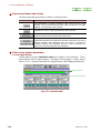
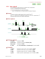
■ Shim-control relation parameters
l Lock signal display
The bar graph in the top of the Shim Control part is called a “lock level meter”. This is
used to monitor the lock signal intensity. The upper of the bar graph is “Coarse” and the
lower is “Fine”. Moreover, the actual lock signal intensity is also displayed numerically.
Lock level meter
Lock signal intensity
Fig. 2.21 Lock level meter
2-26
NMECA/ECX-USM-3
2 SPECTROMETER CONTROL
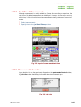
2.3
EXPERIMENT EDITOR TOOL WINDOW
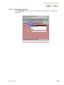
If you click on the Expmnt button in the Spectrometer Control window, the Open
Experiment window that selects a pulse sequence opens. Then, if you select a pulse
sequence, and click on the Ok button, the Experiment Tool window that sets a
measurement parameter will also open.
Fig. 2.22 Open Experiment window
If you select a pulse sequence in the Open Experiment window, and click on the Ok
button, the Experiment Tool window opens.
Fig. 2.23 Experiment Tool window
In the Experiment Tool window, the parameters foe each section Header, Instrument,
Acquisition, and Pulse are set up, and measurement is started by the selecting Submit
button.
NMECA/ECX-USM-3
2-27
2 SPECTROMETER CONTROL
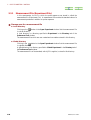
2.3.1
Measurement File (Experiment File)
In this spectrometer, the file in which the pulse sequence was stored is called the
measurement file (Experiment File). A measurement file contains the standard value of a
measurement parameter in addition to a pulse sequence.
■ Storage area for a measurement file
l Local directory
button in the Open Experiment window lists the measurement file
Clicking on the
in a local directory.
A local directory is a directory specified to Experiment in the Directory tab of the
Preferences Tool window.
The measurement files which are user created and corrected are stored in this directory.
l Global directory
button in the Open Experiment window lists the measurement file
Clicking in the
in a global directory.
A global directory is a directory specified to Global Experiment in the Directory tab of
the Preferences Tool window.
The measurement file of the standard, which JEOL supplies, is stored in this directory.
2-28
NMECA/ECX-USM-3
2 SPECTROMETER CONTROL
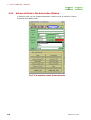
2.3.2
Header Section
In the Header section of the Experiment Tool window, parameters, such as sample_id,
filename, and comment are set.
The Header section has two important functions in addition to this. One is setting a
process list. It specifies which process list is to be used on the data after acquisition.
Another is a header parameter. If you use this function, various spectrometer functions
and data-acquisition conditions can be controlled.
Fig. 2.24 Header section of the Experiment Tool
NMECA/ECX-USM-3
2-29
2 SPECTROMETER CONTROL
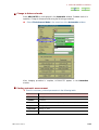
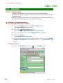
■ Setting process list
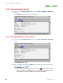
The default process list is described in the measurement file supplied as a standard.
When changing these contents, you can change a process list in the following procedure.
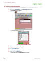
1. Click on the Edit button in the Header section of the Experiment Tool
window.
The Set Process window opens.
Fig. 2.25 Set Process window
2-30
NMECA/ECX-USM-3
2 SPECTROMETER CONTROL
2. Select the kind of process list:
Kinds
Explanation
Process_Ndimensional
The data is sent to 1D Processor or nD Processor after
measurement is complete. However, processing is not
performed.
Process_Local
Data processing is performed using the specified process
list in a local directory after a measurement is complete, and
the result is saved. Neither 1D Processor nor nD
Processor is displayed.
Process_Interactive_Local
Data is sent to 1D Processor or nD Processor after
measurement is complete. Then, the specified process list is
set in a local directory.
Process_Global
Data processing is performed using the specified process
list in a global directory after measurement is complete, and
a result is saved. 1D Processor or nD Processor is not
displayed.
Process_Interactive_Global
Data is sent to 1D Processor or nD Processor after
measurement is complete. Then, the specified process list
in a global directory is set.
Send_data_to_finger
The process list of the data displayed on 1D Processor and
nD Processor is used.
Other()
The program which performs data processing is performed.
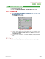
3. Select a process list.
If you click on the Get Process List button, the Select Process List window opens.
Select a process list, and click on the Ok button.
Fig. 2.26 Select Process List window
4. After setting is complete, click on the Accept button in the Set Process
window.
The Set Process window is closed, and a new process list is set in the process of
the Header section of the Experiment Tool window.
NMECA/ECX-USM-3
2-31
2 SPECTROMETER CONTROL
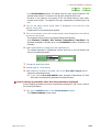
■ Addition of Header parameter
You can add a new parameter to the Header section using the following methods:
1. Click on the Header tab in the Experiment Tool window.
The Header section appears.
2. Click on the
button.
The Include Parameter window opens.
Fig. 2.27 Include Parameter window
3. Select the parameter to add.
The selected parameter is highlighted.
4. Click on the Add button.
5. Repeat steps 3-4 if required.
6. Finally click on the Done button.
The parameter added to the Header section appears.
2-32
NMECA/ECX-USM-3
2 SPECTROMETER CONTROL
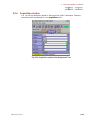
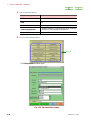
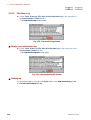
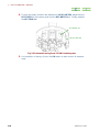
2.3.3
Instrument Section
In the Instrument section, you can set the conditions of an NMR lock, receiver, and
audio filter.
Fig. 2.28 Instrument section of the Experiment Tool
NMECA/ECX-USM-3
2-33
2 SPECTROMETER CONTROL
■ Addition of Instrument parameter
You can add a new parameter to the Instrument section using the following methods.
1. Click on the Instrument tab in the Experiment Tool window.
The Instrument section appears.
2. Click on the
button.
The Include Parameter window opens.
Fig. 2.29 Include Parameter window
3. Select ｔhe parameter to add.
The selected parameter is highlighted.
4. Click on the Add button.
5. Repeat steps 3-4 if required.
6. Finally click on the Done button.
The parameter added to the Instrument section appears.
2-34
NMECA/ECX-USM-3
2 SPECTROMETER CONTROL
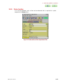
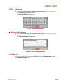
2.3.4
Acquisition Section
You can set the parameters related to data acquisition (NMR observation frequency,
observation width, and data point) in the Acquisition section.
Fig. 2.30 Acquisition section of the Experiment Tool
NMECA/ECX-USM-3
2-35
2 SPECTROMETER CONTROL
■ Addition of the Acquisition parameter
You can add a new parameter to the Acquisition section using the following methods:
1. Click on the Acquisition tab of the Experiment Tool window.
The Acquisition section appears.
2. Click on the
button.
The Include Parameter window opens.
Fig. 2.31 Include Parameter window
3. Select the parameter to add.
The selected parameter is highlighted.
4. Click on the Add button.
5. Repeat steps 3-4 if required.
6. Finally click on the Done button.
The parameter added to the Acquisition section appears.
2-36
NMECA/ECX-USM-3
2 SPECTROMETER CONTROL
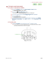
2.3.5
Pulse Section
You can set parameters, such as time and an attenuator that is required for a pulse
sequence in the Pulse section.
Fig. 2.32 Pulse section of the Experiment Tool
NMECA/ECX-USM-3
2-37
2 SPECTROMETER CONTROL
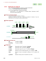
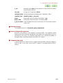
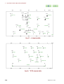
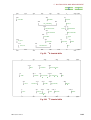
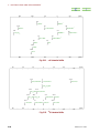
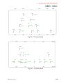
■ Time chart Display of pulse-sequence
You can express the time chart of a pulse sequence as the following procedure:
1. Click on the Pulse tab in the Experiment Tool window.
The Pulse section appears.
2. Click on the
button.
The Pulse Viewer window opens.
Fig. 2.33 Pulse Viewer window
2-38
NMECA/ECX-USM-3
2 SPECTROMETER CONTROL
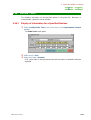
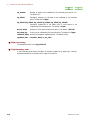
2.4
AUTOMATION TOOL WINDOW
If you click on the Auto button in the Spectrometer Control window, the Automation
window in which all step from measurement of data to processing and printing of data
are automatically performed opens.
In the Automation window, there are the two modes - Standard mode and Advanced
mode.
to the “AUTOMATIC MEASUREMENT” of separate volume for details on
F Refer
automatic measurement.
2.4.1
Standard Mode in the Automation Window
In Standard mode, measurement is performed according to the measurement conditions
of the number of scans to accumulate to repetition time as set as the default in the
automatic measurement template.
Fig. 2.34 Automation window (Standard mode)
NMECA/ECX-USM-3
2-39
2 SPECTROMETER CONTROL
■ Start of automatic measurement
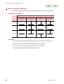
1. Enter the necessary minimal parameters in the following table:
Parameter
Explanation
Filename
Saving file name
Comment
Comment
Slot
Slot number for the auto-sample changer （at auto-sample-changer use）
Temp. Set
Setting temperature for the VT unit
Temp. State
Setting the VT state
Solvent
Solvent
2. Set up arbitrary options.
Typical arbitrary parameter
Explanation
Notify
Transmission place for the measurement completion e-mail
Hold
Holding transmission
completion e-mail
Gradient Shim
Performing gradient shimming
Gradient Optimization
Gradient shimming is performed only when measuring the
first sample or after changing the sample time.
Enhance Filename
A date is added to the file name.
place
of
the
measurement
3. Click on the method button.
Method
?A
method can be continuously recorded like as in a measurement Queue.
However, the order of measurement is the same order, recorded to the measurement Queue. If a new measurement Queue is taken from the Experiment
Tool window during automatic measurement, it will interrupt after the Queue
of the present experiment finishes.
2-40
NMECA/ECX-USM-3
2 SPECTROMETER CONTROL
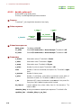
■ Automation window icons
Icon
Button name
Explanation
Open Automation File
The present automatic measurement template is deleted,
and a new automatic measurement template is read.
Include Automation File
A new automatic measurement template is added to the
present automatic measurement template.
Show Queue
The Queue display window for automatic measurement is
opened.
Hide Queue
The Queue display window for automatic measurement is
closed.
Automation Editor
The Automation Editor window is opened.
Run Experiment
Click on this button when performing an experiment, a
check window indicating when measurement is performed
will appear.
? Refer to the “AUTOMATIC MEASUREMENT" of a separate volume for details on
automatic measurement.
NMECA/ECX-USM-3
2-41
2 SPECTROMETER CONTROL
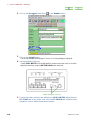
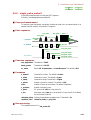
2.4.2
Advanced Mode in the Automation Window
In Advance mode, you can change measurement conditions such as number of scans to
accumulate and repetition time.
Fig. 2.35 Automation window (Advanced mode)
2-42
NMECA/ECX-USM-3
2 SPECTROMETER CONTROL
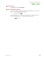
■ Change to Advanced mode
When ADVANCED is not displayed in the Automation window, Standard mode is in
operation. Change to Advanced mode using the following procedures.
u
Select File-Advanced Mode in the menu bar of the Automation window.
After changing procedure is complete, ADVANCED appears in the Automation
window.
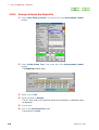
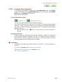
■ Starting automatic measurement
1. Enter the necessary minimal parameters in the following table:
Parameter
NMECA/ECX-USM-3
explanation
Filename
Saving file name
Comment
Comment
Slot
Slot number of the auto-sample changer （at auto-sample-changer use）
Temp. Set
Setting temperature of the VT unit
Temp. State
Setting VT state
Solvent
Solvent
2-43
2 SPECTROMETER CONTROL
2. Set up arbitrary options.
Typical arbitrary parameter
Explanation
Notify
Transmission place for measurement completion mail
Hold
Holding transmission place for measurement completion
mail
Gradient Shim
Performing gradient shimming
Gradient Optimization
A gradient shimming is performed only when measuring
first sample or after changing the sample time.
Enhance Filename
A date is added to the file name.
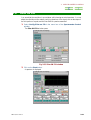
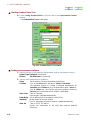
3. Click on the method button.
Method
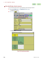
The Set Parameters window opens.
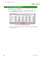
Fig. 2.36 Set Parameters window
2-44
NMECA/ECX-USM-3
2 SPECTROMETER CONTROL
In the Set Parameters window, the setting range for every group contained in the
selected method exists. The range for this group is divided by a blue line.
Moreover, in the range for every group of this, the setting range for every measurement exists further. The range for this every measurement is divided by the red
line.
4. Click on the button whose group name is displayed on the blue line, and
place a check mark.
Measurement for the selected group appears.
5. Click on the button next to the measurement name displayed on the red line
to place a check mark.
The parameter setting range of the selected measurement appears.
Since Filename / Comment / Slot / Solvent / Temperature / Temp.State in the
displayed parameters is already set up in the Automation window, re-setting is not
necessary.
6. Select a parameter to change from the parameter list.
The selected parameter is highlighted, and the input box to the side displays the
value of the present parameter.
7. Change the parameter value.
8. Repeat steps 6-7 if necessary.
9. After parameter change is complete, click on the Run with Changes button.
Automatic measurement starts.
If you click the Run with Default button, automatic measurement will start
after returning measurement parameter to the default value.
?
■ How to change a parameter other than the parameters displayed
When changing parameters other than the parameters displayed in the list box, perform
the following procedure:
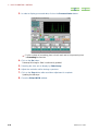
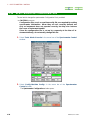
1. Click on the Initialize button in the Set Parameters window.
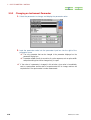
The Choose Parameter window opens.
NMECA/ECX-USM-3
2-45
2 SPECTROMETER CONTROL
Fig. 2.37 Choose Parameter window
2. Select the parameter to add from the Choose Parameter window.
3. Click on the Add button.
4. Repeat steps 2-3 if necessary.
5. Click on the Done button after selecting all the parameters to add.
The Choose Parameter window is closed, and the contents of the parameter list are
updated.
6. Select the added parameter from the parameter list in the Set Parameters
windows.
The selected parameter is highlighted, and the input box to the side displays the
value of the present parameter.
7. Change the value of a parameter.
8. Repeat steps 6-7 if necessary.
9. After parameter change is complete, click on the Run with Changes button.
Automatic measurement starts.
2-46
NMECA/ECX-USM-3
2 SPECTROMETER CONTROL
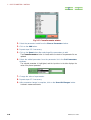
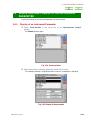
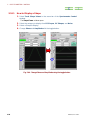
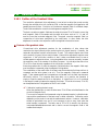
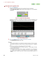
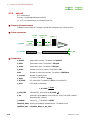
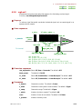
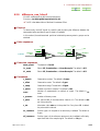
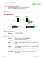
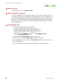
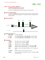
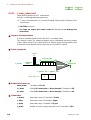
2.5
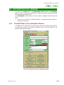
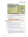
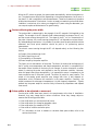
RUN SAWTOOTH EXPERIMENT WINDOW
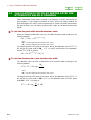
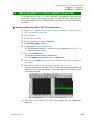
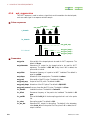
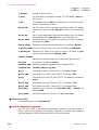
If you click on the Sawtooth button in the Spectrometer Control window, the Run
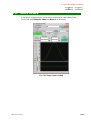
Sawtooth Experiment window that displays a swept lock signal opens.
Fig. 2.38 Run Sawtooth Experiment window
This function is used when verifying a lock signal. When automatic locking does not
function or composition of the deuterated solvent in a sample differs from the normal
(example:10%D20, mixed solvent, and other), this function is used to verify a lock signal.
When exchanging a sample, it is not needed.
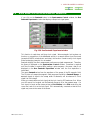
Sawtooth display like other measurement performs one signal measurement. Therefore,
the Queue is displayed on the Spectrometer Control window. Sometime is required
until the first data is acquired after reading a pulse sequence. Moreover, data is not
displayed on the Run Sawtooth Experiment window until the first acquisition is
terminated.
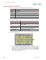
The name Sawtooth arises from the waveform of the sweep of the Z0 magnetic field.
The Z0 shim coil sweeps the magnetic field range specified with a Sawtooth Range. A
sawtooth signal (a signal in the sweep width of sawtooth) will be observed if a lock
signal lies in this range.
When you cannot observe a lock signal, set the Lock Level to 255 maximum first. When
you still cannot find a signal, set the Sawtooth Range to 8 for the greatest range. If a
lock signal is found, set the mouse pointer to Pick Position in the Pick mode using the
cursor tool, and click on the lock signal. Z0 is automatically corrected so that the lock
signal may come to the center of the screen.
NMECA/ECX-USM-3
2-47
2 SPECTROMETER CONTROL
2.6
VECTOR VIEWER WINDOW
If you click on the View button in the Spectrometer Control window, the Vector View
window that displays the spectrum during measurement opens.
Fig. 2.39 Vector View window
The Vector View window has the function which displays a spectrum on real time as the
data monitor during measurement.
If you click on the View button in the Vector View window, the present data is
transmitted from the spectrometer to the screen. In addition, a transmission interval is an
interval specified by mod return in the Acquisition section of the Experiment window.
For example, if the value of mod return is set to 2, data is transmitted for every two
accumulations. A load for a network increases when you shorten the updating interval of
the data. So try to set a suitable value.
? Updating
time for a spectrum in the Vector View window lasts until an
accumulation is terminated from the state where the View button was clicked. If the
updating time of a spectrum exceed 5 minutes, the View button turns OFF automatically. This is for reduces the load to a network. Once again, if you click on the
View button, an updating spectrum is restarted.
? Even if the parameter specified to the mod return parameter is 1, when data points
are too many or Acquisition time and relaxation delay are extremely short, or
when the load of a network is large, an updating spectrum cannot be performed at
the interval specified.
2-48
NMECA/ECX-USM-3
2 SPECTROMETER CONTROL
2.6.1
Changing a Display
This is the method of changing a FID display and a processed data display in the Vector
View window.
1. Click on the Process button in the Vector View window.
It changes to the processed data display.
2. Click on the Process button again.
It returns to the FID display.
NMECA/ECX-USM-3
2-49
2 SPECTROMETER CONTROL
2.6.2
Processing Menu
The contents of processing can be selected in the Vector View window during processed
data display.
u Select the menu displayed in Processing of the menu bar in the Vector
View window.
Processing of the function by which the check mark is placed is them performed.
Function
2-50
Explanation
DC Balance
Corrects the DC component of FID.
Hamming
Multiplies Hamming window.
Zero fill x2
Performs 2 times zero filling
Zero fill x4
Performs 4 times zero filling
FFT
Performs FFT.
Abs
Performs an absolute value display.
Machine Phase
Performs automatic phase correction.
Phase
Performs phase correction.
DC Correct
Performs baseline correction.
NMECA/ECX-USM-3
2 SPECTROMETER CONTROL
2.7
MAKE A NEW INSTANCE OF A SELECTED JOB
COMMAND
You can copy the data in the middle of a measurement, and process it data using 1D
Processor and nD Processor. This function is used when verifying the progress in the
middle of an accumulation.
u Click on the Copy button in the Spectrometer Control window.
The data in the middle of measurement is copied, and 1D Processor or nD Processor starts.
NMECA/ECX-USM-3
2-51
2 SPECTROMETER CONTROL
2.8
90° PULSE WIDTH DISPLAY
90⁰ pulse width for each measurement nucleus and the attenuator value which are
described in a probe file can be displayed.
u Select Tools—90's in the menu bar of the Spectrometer Control window.
90⁰ pulse width display window opens.
Fig. 2.40 90° pulse width display window
? This window can only display the contents of a probe file, and cannot change the
value in the probe file.
2-52
NMECA/ECX-USM-3
2 SPECTROMETER CONTROL
2.9
DISPLAYING AND CHANGE OF AN INSTRUMENT
PARAMETER
Display and change of an instrument parameter can be performed.
2.9.1
Display of an Instrument Parameter
1. Select Tools—Params in the menu bar of the Spectrometer Control
window.
The Params window opens.
Fig. 2.41 Params window
2. Select a parameter to display parameter value with a mouse.
The selected parameter is highlighted, and the value of a parameter is displayed.
Fig. 2.42 Display of the parameter
NMECA/ECX-USM-3
2-53
2 SPECTROMETER CONTROL
2.9.2
Changing an Instrument Parameter
1. Select the parameter to change, and display the parameter value.
2. Input the parameter value into the parameter input box into the right of the
parameter name.
The only parameter that can be changed is the parameter displayed on the
parameter display box.
Parameter related directly to execution of a pulse sequence, such as pulse width
and pulse waiting time can be changed only in a part.
?
?
? If the value of a parameter is changed in this window, since value is immediately
sent to a spectrometer and the state of a spectrometer will its change, cautions are
required even if the spectrometer is under measurement.
2-54
NMECA/ECX-USM-3
2 SPECTROMETER CONTROL
2.10
SHAPE VIEWER
A tool which a Shaped pulse or a noise source can be viewed is provided by Delta.
Three kinds of FG Shape, RF Shape, and Noise can be displayed.
Fig. 2.43 Shape Viewer window
NMECA/ECX-USM-3
2-55
2 SPECTROMETER CONTROL
2.10.1
How to Display a Shape
1. Select Tools—Shape Viewer in the menu bar of the Spectrometer Control
window.
The Shape Viewer window opens.
2. Select the category to display from FG Shapes, RF Shapes, and Noise.
3. Select a Shape to display.
4. Change Phase and Amplitude with the toggle button.
Fig. 2.44 Change Phase and Amplitude using the toggle button
2-56
NMECA/ECX-USM-3
2 SPECTROMETER CONTROL
2.10.2
Calculation of Pulse Width and Attenuator Value
Calculate and display the pulse width and the attenuator value of a shaped pulse in the
Shape Viewer window.
? Only RF Shapes provides a target for calculation.
1. Enter a value into Reference of 90 Pulse and Power Level.
2. Enter a value into Worksheet of 90 Pulse or Power Level.
The remaining value is calculated from the entered value and the Reference value.
NMECA/ECX-USM-3
2-57
2 SPECTROMETER CONTROL
2.11
ABNORMAL DISPLAY OF A SPECTROMETER
u Select Tools—Status in the menu bar of the Spectrometer Control window.
The situation of the alarm of a spectrometer is investigated, and the result is displayed on Delta Console.
Fig. 2.45 Display of the spectrometer alarm on Delta Console
? A transitional error may be reported if this check button is carried out immediately
after starting the system. Perform recheck after carrying out loading of a sample,
NMR lock, and measurement.
2-58
NMECA/ECX-USM-3
2 SPECTROMETER CONTROL
2.12
VALIDATION
This verifies whether software is correctly installed in the spectrometer control computer.
2.12.1 Executing Validation
1. Select Tools—Validation in the menu bar of the Spectrometer Control
window.
The Delta Installation Validation window opens.
Fig. 2.46 Delta Installation Validation window
2. Click on the Go button.
The check of a file is performed and the result is displayed.
Fig. 2.47 Display of Validation result
NMECA/ECX-USM-3
2-59
2 SPECTROMETER CONTROL
2.12.2 Printing Validation Result
u Click on the Print the results button in the Delta Installation Validation
window.
The Validation result is printed to the default printer.
2.12.3 Saving Validation Results to a File
1. Click on the Save the results button in the Delta Installation Validation
window.
The Save file window opens.
2. Input a saving file name into the Name input box after moving to the directory
to save, and click on the Ok button.
The Validation result is saved.
button after specifying
When creating a new saving directory, click on the
a directory name to the Path input box. Create and transfer the directory.
Then, the saving file name is entered into the file name input box.
?
2-60
NMECA/ECX-USM-3
2 SPECTROMETER CONTROL
2.13
DISPLAY OF LOG FILE
This displays the spectrometer log.
Three kinds of Cryogen Log, Machine Log, and Queue Log are saved as a log.
2.13.1
Cryogen Log
u Select Tools—View Log File—View Cryogen Log in the menu bar of the
Spectrometer Control window.
The Cryogen Log window opens.
Fig. 2.48 Cryogen Log window
? A display can be selected from Month, Quarter, and Year.
The display can be
changed by selecting Month, Quarter or Year selecting View from the menu bar in
the Cryogen Log window.
? The front screen or the following screen can be displayed by clicking on the arrow
button.
■ Plotting log
Click on the Plot Cryogen Graph button in the Cryogen Log window to plot the graph.
NMECA/ECX-USM-3
2-61
2 SPECTROMETER CONTROL
2.13.2
Machine Log
u Select Tools—View Log File—View Current Machine Log in the menu bar of
the Spectrometer Control window.
The View machine.log window opens.
Fig. 2.49 View machine.log window
■ Display of an old Machine.log
u Select Tools—View Log File—View Old Machine Log in the menu bar of the
Spectrometer Control window.
The View machine.log.old window opens.
Fig. 2.50 View machine.log.old window
■ Plotting log
A log can be printed by clicking on the Print button in the View machine.log window,
or the View machine.log.old window.
2-62
NMECA/ECX-USM-3
2 SPECTROMETER CONTROL
2.13.3
Queue Log
u Select Tools—View Log File—View Current Queue Log in the menu bar of
the Spectrometer Control window.
The View queue.log window opens.
Fig. 2.51 View queue.log window
■ Display of old Queue.log
u Select Tools—View Log File—View Old Queue Log in the menu bar of the
Spectrometer Control window.
The View queue.log.old window opens.
Fig. 2.52 View queue.log.old window
■ Plotting log,
A log can be printed by clicking on the Print button of the View queue.log window or
the View queue.log.log window.
NMECA/ECX-USM-3
2-63
2 SPECTROMETER CONTROL
2.14
PRE TUNE
When using an autotuning unit, it is necessary to set up the dial value of the probe in
advance. Pre Tune performs these settings.
Pre Tuning is performed by the following procedure.
1. Select Tools—Mode-Console in the menu bar of the Spectrometer Control
window.
2. Select Config—PreTune in the menu bar of the Spectrometer Control
window.
The Config Autotune Probe window opens.
2-64
NMECA/ECX-USM-3
2 SPECTROMETER CONTROL
Fig. 2.53 Config Autotune Probe window
3. Read the dial value of the auto-tuning probe, and enter a dial value into each
input box.
4. Click on the 1H &13C button.
The check window of a dial value appears.
5. Click on the OK button after confirming that the dial value is set correctly.
Dial value is saved and Pre Tuning begins.
Pre Tuning is performed in the order of Coarse, LF, and HF. The following dialog
boxes are displayed during the Pre Tuning of LF and HF.
6. After the dialog box of HF disappears and Pre Tuning is complete, click on
the Close button in the Config Autotune Probe window to close the window.
7. Click on the Connect button in the Spectrometer Control window to return
the connection mode to Connect mode.
NMECA/ECX-USM-3
2-65
2 SPECTROMETER CONTROL
2.15
PROBE TUNE
This performs tuning on the specified nucleus. Although tuning can also be performed at
measurement, when tuning before measurement, tuning is performed by the following
procedure.
1. Select Config—Probe Tune in the menu bar of the Spectrometer Control
window.
The Probe Tune Tool window opens.
Fig. 2.54 Probe Tune Tool] window
2. Select the coil to tune in Coil.
3. Select the nucleus to tune in Domain.
4. Set an Offset if necessary.
5. Click on Force Tune.
Unless a check mark is placed in Force Tune, the tuning of a nucleus which has
already been tuned is not performed.
6. Click on the Tune Now button.
Tuning starts.
7. Click on the Close button after tuning is complete.
The Probe Tune Tool window closes.
2-66
NMECA/ECX-USM-3
2 SPECTROMETER CONTROL
2.16
PROBE TOOL
This displays information on the specified nucleus in the probe file. Moreover, in
Console mode, a probe file can be rewritten.
2.16.1
Display of Information for a Specified Nucleus
1. Select Config—Probe Tool in the menu bar of the Spectrometer Control
window.
The Probe Tool window opens.
2. Select a coil in Coil.
3. Select a nucleus in Domain.
A 90° pulse width for the specified nucleus and information on attenuator value are
displayed.
NMECA/ECX-USM-3
2-67
2 SPECTROMETER CONTROL
2.16.2
Saving a Value to the Probe File
1. Select Tools—Mode—Console in the menu bar of the Spectrometer Control
window.
2. Select Config—Probe Tool in the menu bar of the Spectrometer Control
window.
The Probe Tool window opens.
3. Select a coil in Coil.
4. Select a nucleus in Domain.
The 90° pulse width of the specified nucleus and information on attenuator value
are displayed.
5. Correct value.
6. Click on the Save Probe File button.
The probe file is updated.
2-68
NMECA/ECX-USM-3
2 SPECTROMETER CONTROL
2.17
SHIM ON FID
You can adjust the resolution in one window while viewing an actual spectrum. You can
adjust the resolution while actually verifying situations of the signal, such as the shape of
the skirt portion of a peak, and the line width of a peak as measured.
1. Select Config—Shim on FID in the menu bar of the Spectrometer Control
window.
The Shim ON FID window opens.
Fig. 2.55 Shim ON FID window
2. Click on the Start button.
A spectrum is displayed.
NMECA/ECX-USM-3
2-69
2 SPECTROMETER CONTROL
3. In order to display processed data, click on the Process Vector button.
? For the contents of processing, place a check mark next to the processing item
in Processing the menu bar.
4. Click on the Go button.
Data acquisition begins. Data is continuously updated.
5. Selecting the shim axis to display by Shim Group.
6. Adjust the resolution while viewing a spectrum.
7. Click on the Stop button after resolution adjustment is complete.
Updating the data stops.
8. Close the Shim ON FID window.
2-70
NMECA/ECX-USM-3
2 SPECTROMETER CONTROL
2.18
GRADIENT SHIM TOOL
2.18.1 Outline of the Gradient Shim
The resolution adjustment (shim adjustment) is carried out to adjust the current running
through the multiple shim coils inside the SCM so that the magnetic field applied to the
sample becomes uniform. Each shim coil produces a magnetic field of a different shape.
These fields are added to correct the inhomogeneous magnetic field.
The basic correction magnetic fields are the axial shim terms Z1 to Z6 used to correct the
axial magnetic field of the sample and the radial shim terms such as X1, Y1, and XZ
used to correct the horizontal magnetic field. The actual correction magnetic field is a
composition of shim terms multiplied by the coefficients. In other words, the shim
adjustment is carried out to adjust the coefficient applied to these shim terms.
■ Feature of the gradient shim
Conventional shim adjustment searches for the combination of shim values that
maximizes the signal intensity while monitoring the lock signal intensity. Generally, the
automatic adjustment function called simplex is used. This method requires more time
as the number of types of shims used increases. Manual shim adjustment requires some
experience. If the initial shim condition is bad, it takes considerable time for even a
skilled operator to adjust the shims. Using the gradient shim, anyone can easily increase
the resolution, even if the number of the shims increases. You can adjust the shims from
Z1 to Z6 in a few minutes, regardless of the initial shim conditions.
When the gradient shim is used, the magnetic field distribution (the magnetic field map)
over the sample is measured using the magnetic field gradient.
The combination of the coefficients of the basic map that makes the field map uniform is
computed, and the shim system is set to it. Then, the magnetic field map is measured
again. These measurements and computations are iterated until the field map becomes
sufficiently uniform. The computer does these tasks, so in practice, the operation is
simply to insert the sample and click on the button. A single line of 2H or 1H contained
in the sample is used to measure the magnetic field map. The axial shim terms, Z1 to Z6,
can be adjusted as the Field gradient of the Z1 axis is used.
? Calibration (creating the basic map)
When the gradient shim is used, the shim terms Z1 to Z6 are calculated based on the
correction magnetic field.
The correction magnetic field measured using the standard sample is called the basic
map, and the measurement of the basic map is called calibration. Calibration varies
depending on the probe in use and the measurement nucleus. However, calibration
should be performed once, and it is not necessary to do so every time when the
actual sample is measured. The basic map of Z1 to Z6 is stored in the directory
/usr/people/delta/delta/instrument and is used to correct the magnetic field of the
measurement sample.
NMECA/ECX-USM-3
2-71
2 SPECTROMETER CONTROL
■ Gradient shim
In the gradient shim used in the spectrometer, there are two methods for homogeneity
spoiling (homospoil) and PFG (Pulsed Filled Gradient). In this spectrometer, the
homogeneity spoiling gradient shim, whose observed nucleus is 2H, is provided as a
standard, and the conditions that can be used the standard gradient shim for every probe
is set. Moreover, the function in which the gradient shim can be easily performed only
by clicking on an icon is also provided. A gradient shim is recommended if it satisfies
these two conditions:
• The 2H nucleus of a deuterated solvent can be used as an observed nucleus.
• Homogeneity spoiling can be applied for all spectrometers and probes.
? Solvent
• A Selective Gradient is used for gradient shimming of the solvent containing two
or more 2H signals like methanol-d4 or pyridine-d5. In a Selective Gradient, caliseparate volume “ADMINISTRATOR’S MANUAL”).
bration is required (
• In the case of a normal water sample, since sensitivity of the D2O signal is insufficient for a lock, an observed nucleus uses 1H. In a 1H gradient shim, calibration is
separate volume “ADMINISTRATOR’S MANUAL”).
required (
F
F
2-72
NMECA/ECX-USM-3
2 SPECTROMETER CONTROL
2.18.2
Gradient Shim Operation
In the gradient shim operation, a method using the Gradient Shim button of the Sample
window or a method using the Gradient Shim Tool can be used. Usually, the Gradient
Shim button of the Sample window is used.
Each feature is shown below.
l The Gradient Shim button
Gradient Shim button
Gradient Shim and Lock button
Click on one of above buttons to perform gradient shimming.
The Gradient Shim and Lock button turns on the NMR lock after executing gradient
shimming. Usually, sufficient resolution can be obtained by operating these buttons.
Early shim conditions are read from the system shim file. The conditions of the gradient
shimming are fixed.
Refer to Subsection 2.2.7 “■NMR lock control button” for more information on
the usage.
F
l Gradient Shim Tool
Gradient shimming is performed under specified conditions. Change of the resolution
can be verified by display of a magnetic field map. This gradient shim tool is used when
good resolution cannot be obtained by the function of the above button, and when
performing gradient shimming other than on a standard.
■ Preparation
Preparation before beginning gradient shimming is as follows. First load a sample into
the SCM.
1. Open the Sample window and turn ON a spinner.
2. Specify a lock solvent from the Solvent list box.
3. Turn OFF an NMR lock.
NMECA/ECX-USM-3
2-73
2 SPECTROMETER CONTROL
■ Starting Gradient Shim Tool
u Select Config—Gradient Shim in the menu bar of the Spectrometer Control
window.
The Gradient Shim Tool window opens:
Fig. 2.56 Gradient Shim Tool window
■ Setting measurement conditions
1. Specify the type of the magnetic field gradient, and an observation nucleus.
System Type: Homospoil is turned ON.
Nucleus:
2H (Deuterium) is turned ON.
2. Specify other measurement conditions.
Scans:
X Offset:
Set the number of scans to accumulate (4 multiples).
Click on the Once button, and turn on Twice and Calculate.
The resonance position of a signal is searched automatically by
Calculate, and X Offset sets it to the observation center. Once corrects X Offset only once before performing gradient shimming.
Twice adjusts it finely after the 1st iteration is terminated.
Recvr Gain: Turn on Calculate.
Receiver gain is adjusted automatically.
Relax Delay: Set the waiting time of the repetition pulse (5-8s).
Iterations: Set the number of times of iteration.
If it is 0, the number of times of iteration is judged automatically.
Turn on Z1, Z2, Z3, and Z4.
Shim Set:
Specify the combination of the shim that performs gradient
shimming.
2-74
NMECA/ECX-USM-3
2 SPECTROMETER CONTROL
Range/%Width:
Usual measurement does not change. When [%Width] is 100%
(when not specified), and When you use the sample whose liquid
amounts are different such as micro cell, input the effective range
refer to the subsequent page).
which performs gradient shimming (
3. Turn ON Display Field Map.
F
Whenever 1 iteration is terminated, the magnetic field map is displayed. When
Display Field Map is OFF, a map is not displayed.
4. Turn ON AutoLock.
Autolock is applied after you finish gradient shimming.
NMECA/ECX-USM-3
2-75
2 SPECTROMETER CONTROL
■ Start and end of a gradient shim
1. Click on the Start button.
Gradient shimming starts and the job of gradient shimming is performed.
The Gradient Shim Status window opens, and the progress (in %) of the iteration
is displayed.
Fig. 2.57 Gradient Shim Status window
Whenever one iteration is terminated, the magnetic field map is displayed on the
Field Map window. When several iterations are performed, they are all displayed.
Fig. 2.58 Field Map window
2. Click on the Exit button after Gradient Shimming is complete.
The Gradient Shim Tool window closes.
Reference:
• When a good resolution is not obtained, increase the number of scans to accumulate. When the resolution is bad at the start, set many iterations (e.g., 3 instead of
0).
• Usually try to specify the shim settings for Z1, Z2, Z3, and Z4.
• Do not change parameter values during an operation. If they change, the measurement will be influenced.
• In the gradient shimming, a uniform sample is presupposed. If the homogeneity
of a sample is bad, operation of the gradient shim will be affected. Especially
when the solvent is water, take care to remove ant small bubble founded in a
sample.
2-76
NMECA/ECX-USM-3
2 SPECTROMETER CONTROL
• In order to determine the effective range of the magnetic field map, set %Width to
1, set Iterations to 100%, and turn ON Display Field Map, then perform gradient
shimming. The flat portion of the magnetic field map becomes the effective range.
In order to make a percent display for the horizontal axis of the magnetic field
map, select Ruler–Percent in the menu with the right mouse button.
NMECA/ECX-USM-3
2-77
2 SPECTROMETER CONTROL
2.19
SPECTROMETER CONFIGURATION
The tool which changes the spectrometer Configuration file is provided.
—— CAUTION ———————
Configuration files, such as machine.config file, are required for setting
spectrometer information. When they are not correctly defined, not
only an instrument does not operate correctly, but they also become
the cause of instrument trouble.
Since the configuration file is set up by commonly at the time of instrument delivery, do not usually change this file.
1. Select Tools—Mode—Console in the menu bar of the Spectrometer Control
window.
2. Select Config—Machine Config.. in the menu bar of the Spectrometer
Control window.
The Spectrometer Configuration window opens:
2-78
NMECA/ECX-USM-3
2 SPECTROMETER CONTROL
3. Select the file to edit from the Configure Files list box.
4. Click on the Edit button.
The Machine Configure window opens.
5. Select the parameter to change from the Parameter list box.
6. Set a value in the Value input box.
7. Save a file to the Save Configure File (updating).
NMECA/ECX-USM-3
2-79
2 SPECTROMETER CONTROL
2.20
EXPERIMENT AND QUEUE MANAGMENT
Queuing performs measurement in this spectrometer. That is, more than one experiment
can be registered to the spectrometer (submit); and they are performed in the order of
registration. There are five modes OWNED, RUNNING, HALTED, FREE, and
WAITING in the spectrometer Queue. These modes cannot be changed if there is no
console privilege.
A priority is given the measurement that is recorded in a Queue, respectively. The
priority is ranked with numerical values from 0 (minimum) to 255 (maximum). Each
user's default priority is specified as the "queue.priorities" file of the spectrometer
management computer. A user can also change the priority of this measurement.
However, possible change in ranking is only from higher to lower. If you have any
console privilege, you can freely change the priority of all measurements.
2.20.1
Queue State
The present state of the Queue is displayed on the Spectrometer Control window.
State of Queue
Fig. 2.59 State display of Queue
2-80
NMECA/ECX-USM-3
2 SPECTROMETER CONTROL
Hereafter, each state is explained:
State
Occupancy
Display
OWNED
Measurment RUNNING
axplanation
In the state where the system is connected with the spectrometer
using the Connect button, a user can occupy a Queue (it is
owned). Though other users record a measurement (experiment),
only the user who connected previously using the Connect
button can perform a measurement.
In this state another user is performing measurement. Console
privilege is required when changing the Queue.
Stop
HALTED
In this state, the Queue was stopped using the Stop command or
Hold flag. If the Queue is restarted using the Start command, all
measurements will restart.
Free
FREE
Queue is in a free state.
Waiting
WAITING
Measurement start time has been specified, and is in the state of
waiting for an execution.
NMECA/ECX-USM-3
2-81
2 SPECTROMETER CONTROL
2.20.2
Queue Menu
The command for controlling a Queue is provided in the Queue menu of the
Spectrometer Control window.
Fig. 2.60 Queue pull down menu
Menu
2-82
Detail
Start
Restarts a Queue stopped.
Stop
If you execute the Stop command after clicking to select a specified Queue, all
subsequent Queues will be in a pause state.
Since the function of the Stop command differs from the
button, be careful.
Reschedule
The measurement that came to a head can be turned to the end of the Queue. It
is used when a spectrometer is not ready with a certain reason.
Delete
The whole Queue is canceled except for the currently running measurement
Print
The recorded Queue is printed.
NMECA/ECX-USM-3
2 SPECTROMETER CONTROL
2.20.3
Restating Measurement (GO button)
Go button
Before performing the first experiment in the Queue, a spectrometer compares the name
(sample_id) of the last measurement and measurement that it is going to perform from
now. If the sample_id is the same, measurement is started immediately. When the
sample_id is not on agreement or is not specified, measurement will be in the state of
waiting for execution, and a message window will be displayed on a screen.
Here, the states of a sample (spinning of a sample tube and states of a shim) can be verified.
If you click on the GO button, a pause state is canceled and measurement restarts.
Fig. 2.61 Check message window
Measurement that changes into waiting state for an execution with the Queue is as
follows. Observe “–” displayed on the top line.
Fig. 2.62 Measurement (Spectrometer Control window) for an execution
waiting state
NMECA/ECX-USM-3
2-83
2 SPECTROMETER CONTROL
If you click on the GO button, the following appears. Observe that “–” changes to “* ”.
Fig. 2.63 Restarting measurement (Spectrometer Control window)
2-84
NMECA/ECX-USM-3
2 SPECTROMETER CONTROL
2.20.4
Cancelling Measurement (STOP button)
STOP button
The experiment that recorded in a Queue can be canceled using the following procedure.
1. Select the measurement to cancel.
Highlighted by
selecting
Fig. 2.64 Selection of a measurement (Spectrometer Control window)
2. Click on the STOP button.
Several seconds are required before measurement is canceled by the state of a network
and measurement repetition time. When save aborted of the Experiment flag was True,
data is read while having been canceled and it is displayed on the 1D Processor window.
Data is deleted when it is not True. This flag is True unless the setting is changed.
NMECA/ECX-USM-3
2-85
2 SPECTROMETER CONTROL
2.20.5
Measurement Priority
As described above, priorities from 0 to 255 exist in a measurement (experiment), and a
measurement priority already recorded in a Queue can be changed in the Spectrometer
Control window. If you select measurement and input a numerical value in the Priority
input box, the order of measurement will change according to the priority. However,
change of a common user's priority is only the change to the lower one. Measurement
priority can be changed freely by a privilege user.
? Change to Queue under measurement cannot be performed now.
Priority
Input box
Fig. 2.65 Priority input
2.20.6
Slot
The Slot input box is specified when using an auto sample changer.
2-86
NMECA/ECX-USM-3
2 SPECTROMETER CONTROL
2.20.7
Start Time of Measurement
Although measurement is usually added to a Queue after recording an experiment, the
start time of the added measurement can be delayed. However, since an error can occur
at this time, it differs from the time when measurement actually starts tens of seconds to1
minute.
1. Select measurement.
2. Specify time to the Job Start Time input box.
Fig. 2.66 Input of measurement start time
2.20.8 Measurement Information
If you double-click on the experiment displayed on the Spectrometer Control window,
the Job Info window that displays information about measurement opens.
Fig. 2.67 Job Info
NMECA/ECX-USM-3
2-87
2 SPECTROMETER CONTROL
2.21
2.21.1
APPENDIX
Probe Tuning
The tuning method of the TH5AT/FG2 probe will be explained as an example.
When turning on the power supply of the auto-tuning unit, the TH5AT/FG2 probe can be
tuned automatically.
When turning off the power supply of the auto-tuning unit, and removing the flexible
shaft, the TH5AT/FG2 probe tuning can be performed as follows.
■ 1H tuning in normal measurement
l To set the 1H measurement conditions
1. Click on the Expmnt button in the Delta Console window.
The Open Experiment window appears.
2. Click on the
Global Directory button.
The contents of the Global Experiment directory are displayed.
3. Click on the measurement mode single pulse.ex2 to highlight it.
4. Click on the Ok button.
The Experiment Tool window appears.
5. Set each parameter for normal 1H measurement in sequence in the Header,
Instrument, Acquisition, and Pulse sections in the Experiment Tool
window.
l Tuning the probe
1. Click on the force tune check box (
2-88
) in the Header section.
NMECA/ECX-USM-3
2 SPECTROMETER CONTROL
2. Click on the Submit button.
The tuning message is displayed as shown below. At this time, the probe has
already been set to tuning.
3. Set the tuning sensitivity.
If the LEVEL METER on the head amplifier chassis moves too much or too little,
adjust the sensitivity using the METER GAIN button and knob.
METER GAIN button and knob
Fig. 2.68 Display panel of the head amplifier chassis
NMECA/ECX-USM-3
2-89
2 SPECTROMETER CONTROL
4. To tune the probe, minimize the deflection of LEVEL METER. Adjust first the
HF1 TUNE dial of the probe, and next the HF1 MATCH dial. Finally, readjust
the HF1 TUNE dial.
HF1 MATCH dial
HF1 TUNE dial
Fig. 2.69 Automatic-tuning 5 mm FG NMR tunable probe
5. On completion of tuning, click on the GO button to start normal 1H measurement.
2-90
NMECA/ECX-USM-3
2 SPECTROMETER CONTROL
■
13
C tuning in normal measurement
l To set the 13C measurement conditions
1. Click on the Expmnt button in the Spectrometer Control window.
The Open Experiment window appears.
2. Click on the
Gloval Directory button.
The contents of the Global Experiment directory are displayed.
3. Click on the measurement mode single pulse dec.ex2 to highlight it.
4. Click on the Ok button.
The Experiment Tool window appears.
5. Set each parameter for normal 13C measurement in sequence in the Header,
Instrument, Acquisition, and Pulse sections in the Experiment Tool
window.
l To tune the probe
1. Set the LF COARSE knob of the probe to the 13C frequency range.
? For the values of tuning and matching dials for the observation nucleus, refer to
the table provided with the TH5AT/FG2 probe.
LF COARSE knob
NMECA/ECX-USM-3
2-91
2 SPECTROMETER CONTROL
2. Click on the force tune check box (
) in the Header section.
3. Click on the Submit button.
The tuning messages are displayed. First, the 13C tuning message is displayed.
4. Set the sensitivity of tuning.
If the LEVEL METER on the head amplifier chassis moves too much or too little,
adjust the sensitivity using the METER GAIN button and knob.
METER GAIN button and knob
5. To tune the probe, minimize the deflection of LEVEL METER. Adjust first the
LF1 TUNE dial of the probe, and next the LF1 MATCH dial. Repeat these
operations until no further improvement results.
2-92
NMECA/ECX-USM-3
2 SPECTROMETER CONTROL
LF1 MATCH dial
LF1 TUNE dial
6. On completion of tuning, click on the GO button.
After the 13C tuning is complete, the 1H tuning message appears. At this time the
probe has already been set to tuning.
7. Perform the 1H tuning.
8. On completion of 1H tuning, click on the GO button to start normal
13
C
measurement.
NMECA/ECX-USM-3
2-93
2 SPECTROMETER CONTROL
■ Precise 13C tuning
1. Turn the LF1 MATCH dial to minimize the deflection of LEVEL METER.
2. Turn the LF1 TUNE dial to minimize the deflection of LEVEL METER.
3. Turn the LF1 MATCH dial by +10 graduations and turn the LF1 TUNE dial to
minimize the deflection (F1) of LEVEL METER.
Memorize the deflection (F1) of LEVEL METER at that time.
4. Turn the LF1 MATCH dial by −10 graduations and turn the LF1 TUNE dial to
minimize the deflection (F2) of LEVEL METER.
Compare the deflection (F2) of LEVEL METER at this time with F1. Turn the
LF1 MATCH dial to minimize the deflection of LEVEL METER, and then turn
the LF1 TUNE dial to minimize the deflection of LEVEL METER.
2-94
NMECA/ECX-USM-3
2 SPECTROMETER CONTROL
2.21.2
Array Measurement
When you perform array measurement, there are parameters whose values are changed in
some order. They are called the array parameters.
This section describes the methods of setting the array parameters in the Experiment
Tool window. Array measurement can be carried out in the same way as ordinary
measurement by clicking on the Submit button.
There are the two methods of setting the array parameters as described below:
• Entering a numerical value into the parameter input box directly
• Using the array parameter window
Array parameter notation
Most of measurement parameters can be used as array parameters using the y_acq
command for 1D measurement. The character y indicates that the array parameters
form the temporary y_domain of 2D data sets.
The array parameters for 2D measurement are also represented as z_acq, and form
the temporary z_domain of 3D data sets.
This section describes array measurement in the single_pulse.ex2 window.
F For explanation about Array data processing, refer to the Processing User’s Manual.
■ Preparation before setting array parameters
1. Select the measurement mode from the Open Experiment window, and click
on the Ok button.
The Experiment Tool window opens.
2. Enter the parameters, such as filename and sample_id.
NMECA/ECX-USM-3
2-95
2 SPECTROMETER CONTROL
■ Entering a numerical value into the parameter input box directly
The format for input into the parameter input box is
y_acq{value1, value2, value3..........}
Array parameter values enclosed with braces { } follow y_acq, and allow any numerical
values or numerical values varying with a constant difference.
Example: x_90_width parameters
To enter numerical values varied with a constant interval in a range, the format is
y_acq{start value ->stop value : step size}
To enter a parameter having a unit, enter the unit with at least one numerical value.
If you specify only one unit, the unit is applied to all numerical values.
At the end of input, press the Enter key or move the mouse pointer outside the window.
If an error is detected in the array parameters, a message is displayed.
To change the numerical values in the parameter input box, move the mouse pointer into
the input box, and correct them using the arrow keys or the backspace key.
To enter a long array, scroll the end of the window. To return to the beginning after
scrolling, use the Home or End key.
You can use both y_acq and z_acq simultaneously. In this case, first, the y_acq array is
executed using the z parameter values, then the y_acq array is executed with the
increment of the z parameter, and these steps are repeated, resulting in pseudo 3D data.
2-96
NMECA/ECX-USM-3
2 SPECTROMETER CONTROL
■ Using the array parameter window
The procedure for setting the scans parameter is described as an example.
1. Double-click on the scans button of the Experiment Tool window.
The array parameter window opens.
Fig. 2.70
Array parameter window
2. Select the Y check button by clicking on it.
3. Enter the parameter values one by one into the numerical input box.
Check button
Numerical-value
list
Numerical-value
input box
Numerical-value
input format
4. To enter the values in a range, click on the Listed check button to turn it off.
5. Select Array Type from Linear, Exponential, and Logarithmic.
The example of x_90_width parameters is shown below.
NMECA/ECX-USM-3
2-97
2 SPECTROMETER CONTROL
Selecting Linear
If you select Linear, enter the values of Start, Stop, and Step in the input boxes. In
the above example, the parameter varies linearly from 1[us] to 16[us] with a 1[us]
interval, that is, 1, 2, 3......14, 15, and 16 [us] (16 points in total).
Selecting Exponential
If you select Exponential, enter the values of Start, Stop, and Points in the input
boxes. In the above example, the parameter varies exponentially from 1[us] to
16[us] with the three-point interval, that is, 1, 4, and 16 [us].
2-98
NMECA/ECX-USM-3
2 SPECTROMETER CONTROL
Selecting Logarithmic
If you select Logarithmic, enter the values of Start, Stop, and Points in each input
box. In the above example, the parameter varies logarithmically from 1[us] to
16[us] with the three-point interval, that is, 1, 12.40116, and 16 [us].
6. Click on the Set Value button.
The following figure shows the setting of the parameter input box in the Experiment Tool window.
l Reference: The method of entering numerical values from the geometry into the
array parameters window
You can enter the numerical values from the data (geometry) displayed on the screen into
the array parameters window.
The procedure is explained using the irr_offset parameter as an example.
1. Select Pick—Copy position to buffer from the cursor tool bar.
2. Move the mouse pointer onto the spectrum displayed on the screen, and
click the left mouse button on the peak set to irr_offset.
The peak position is copied.
3. Move the mouse pointer to the numerical value input box in the array
parameters window, and click on the middle mouse button.
The copied position is pasted, and the numerical value is entered into the list box.
4. Repeat the copy and paste operation, and enter the numerical values into the
list box.
? Ÿ You can perform array measurement only if the array parameter window opens
when you click on the item.
• You cannot use the parameters related to the size of files and the sampling points
as the array parameters, for example, domains, sweep widths, and points.
If you want to change these parameters and perform successive measurements,
use the ordinary queue.
NMECA/ECX-USM-3
2-99
ADJUSTMENT OF
NMR PARAMETERS
The greatest feature of the pulsed NMR method is that various informations can be
derived from spectra which are affected by applying combinations of pulses (pulse
sequences). The nuclear magnetization can be controlled by the pulsed RF excitation. To
manipulate the magnetization precisely, you must set the parameters for controlling the
magnetization. Chapter 3 explains the procedures for these operations.
3.1 PURPOSE OF MEASURING PULSE WIDTHS ......................................... 3-1
3.2 SPECTROMETER RF SYSTEM AND FACTORS AFFECTING
PULSE WIDTHS ....................................................................................... 3-3
3.3 MEASUREMENT OF PULSE WIDTHS WHEN OUTPUT IS
USED AT HALF POWER ......................................................................... 3-5
3.4 CALCULATION OF 90° PULSE WIDTHS AFTER THE
ATTENUATOR VALUE IS CHANGED ................................................... 3-8
3.5 MEASUREMENT OF PULSE WIDTHS IN DEPT90 ................................. 3-9
3.6 CALCULATION OF 90° PULSE WIDTH OF SELECTIVE
EXCITATION PULSES ........................................................................... 3-10
3.7 USAGE OF Attenuator Calculator TOOL ................................................... 3-12
NMECA/ECX-USM-3
3 ADJUSTMENT OF NMR PARAMETERS
3.1
PURPOSE OF MEASURING PULSE WIDTHS
This section explains the significance and principle of measurement of pulse widths, and
general precautions.
■ About pulse width
When an RF pulse having the magnetic-field strength B1 is applied to the magnetization
M in a rotating frame, the magnetization will precess about the axis along the direction of
the applied RF pulse with the angular velocity γB1 (rad/s), where γ is the magnetogyric
ratio.
Z
Flip angle
M
γB1△t
△t
RF pulse
Y’
B1
X’
Fig. 3.1 Precession of magnetization in the rotating frame
As a consequence, if the RF pulse width (the duration of the RF pulse) is △t (s), the
magnetization after the pulse is then related to the magnetization after the pulse by the
flip angle thus:
Flip angle = γB1△t (rad)
In the NMR terminology, the RF pulse width resulting in a flip angle X° is called the X°
pulse width, and the pulse itself the X° pulse.
To carry out precise NMR measurement, it is essential for you to know the
magnetic-field strength of the RF pulse. However, in the pulsed NMR spectrometer, it is
more convenient to use the 90° pulse width PWπ/2 than to use the field strength B1
directly, so that when the magnetic field strength of the RF pulse is referred to, generally
PWπ/2 is used. If PWπ/2 is known, B1 can be computed by the following equation:
B1 = π / (2 × γ × PWπ/2)
■ Principle of measurement of pulse widths
The saturation magnetization is a vector parallel to the Z axis. If the saturation
magnetization is M0, and after the RF pulse with width △t and strength B1 is applied to
the saturation magnetization, the observed signal intensity is
M(△t) = M0 sin (γB1△t)
Thus, the 90° pulse width is the value of △t at which the signal intensity becomes a
maximum when △t is gradually increased. However, in practice, it is much easier to
find the position where the signal intensity becomes zero, so first find the 180° pulse
NMECA/ECX-USM-3
3-1
3 ADJUSTMENT OF NMR PARAMETERS
width and then estimate the 90° pulse width as half its duration, or first find 360° pulse
width and then estimate the 90° pulse width as one fourth of its duration.
M
⊿t
PW90
PW180
PW360
Fig. 3.2
Relationship between the time the RF pulse is applied and the
observed signal intensity
■ Effects of inhomogeneity of the RF magnetic field strength B1
In the previous paragraph, it was assumed that the homogeneous RF magnetic field B1
was applied to the entire sample. In practice, however, depending on the shape of the coil
for generating the RF magnetic field and the sample position relative to the coil, RF
magnetic fields having various strengths are applied to the sample. As a result, the
observed signal intensity is not a simple sinusoidal function of the duration of the RF
pulse. Therefore, more accurate value can be obtained by finding 360° pulse width and
then estimating the 90° pulse width as one fourth of its duration.
3-2
NMECA/ECX-USM-3
3 ADJUSTMENT OF NMR PARAMETERS
3.2
SPECTROMETER RF SYSTEM AND FACTORS
AFFECTING PULSE WIDTHS
In order to adjust the power of the RF pulse or to measure the pulse width, it is necessary
for you not only to learn the procedure for measurement but also to understand the flow
of RF pulses in the spectrometer. You can understand the meaning of the measurement
procedure from understanding the flow of the RF pulses. This section describes the flow
of the RF pulses in the spectrometer and various factors affecting the pulse widths.
■ Outline of the spectrometer RF system
In order to help you to understand the operation of the pulse sequence, a simplified
schematic diagram of the RF system in the spectrometer is shown in Fig. 3.3.
Receiver
Preamplifier
Sequencer
DDS
Transmitter
Sequencer
DDS
Transmitter
Sequencer
DDS
Transmitter
HF power
amplifier
Duplexer
LF power
amplifier
Duplexer
Probe
Dual FSY
Fig. 3.3
Block diagram of the RF system
The standard probe provided with the spectrometer is a tunable double-resonance probe.
This probe can be tuned to the 1H resonance frequency and the resonance frequencies of
nuclei in the range from 31P to 15N. The channel into which RF power at the 1H frequency
is entered is called the HF (High Frequency) channel, and the other channel the LF (Low
Frequency) channel. Do not confuse the HF and LF channels with the observation and
irradiation channels. The HF or LF channel from which a signal at the frequency of an
nucleus being observed is output is called the observation channel. The other channel is
called the irradiation channel.
The signals output from the sequencer are converted to pulses in the DDS. After they are
modulated, they enter into the transmitter. At the same time, the pulses from the dual
FSY enter the transmitter, and are mixed there to produce the RF pulses. The intensity of
the RF pulses can be changed in 1 dB steps by the amplitude control in the DDS, and in
0.01 dB steps by the attenuator in the transmitter, allowing very fine adjustment. When
you enter a value in the attenuator box, the attenuation can automatically be adjusted by
the above devices, so usually you do not care about them. The RF pulses output from the
transmitter are entered into either the HF or the LF power amplifier. The RF pulses are
amplified in the power amplifier, and are entered into the corresponding channel in the
probe. The host computer selects the HF or the LF channel as the observation channel.
The strong RF pulses are applied to the observation channel through the duplexer. After
the strong RF pulses are switched off, the weak observation signals are received by the
probe. The signal from the probe is amplified in the preamplifier, and reaches the
receiver. The RF pulses are also applied to the irradiation channel through the duplexer.
NMECA/ECX-USM-3
3-3
3 ADJUSTMENT OF NMR PARAMETERS
When the RF pulses are output, the spectrometer automatically selects the sequencer to
use. The output power differs a little, depending on the selected sequencer, but its error is
less than 3 %, and is negligible in actual measurement. Therefore, measure only the pulse
width when observation is carried out. You do not need to measure the pulse width when
irradiation is carried out. Also, when you change the RF power using the attenuator, you
can compute a pulse width because of its good linearity.
■ Factors affecting the pulse width
The pulse width is determined by the strength of the RF magnetic field applied to the
sample. The strength of the RF magnetic field is determined by the shape of the RF coil
and the current running through the coil. The shape of the RF coil is a characteristic of
the probe. However, the current running through the RF coil depends on various factors.
By understanding these factors, it is possible to consider when the pulse width should be
measured, and what points attention should be paid to for performing precise
measurement.
The electric current running through the RF coil depends mainly on the following four
factors:
(a) Design of the probe tuning circuit
(b) State of the tuning circuit
(c) Susceptibility of the sample
(d) Power output by the power amplifier
The factor (a) is a characteristic of the probe. The factor (b) varies with the frequency of
the RF pulse, room temperature, and sample temperature, and with (c) susceptibility of
the sample. When the state of the tuning circuit changes, it can be corrected to a certain
extent by retuning the probe, and returned to near the optimum condition. However,
when the sample has a large susceptibility, it is impossible to return it completely to the
same conditions even if the probe is tuned. The factor (d) varies for many reasons. The
output of the analog power amplifier may change with time. It also depends on
temperature, which influences the transistors in the power amplifier. Generally, the
output increases with a decrease in temperature. It is also frequency-dependent. Signals
entered into the power amplifier are most likely influenced by temperature and elapsed
time as well.
■ Pulse widths to be adjusted or measured
Precise pulse widths have been preset in the spectrometer at the time of installation.
However, they may change due to various conditions. When they change, adjust or
measure the following pulse widths:
• Pulse width when you use output at half power
• Pulse width when you change an attenuator value
• Pulse width when you measure DEPT90
• Pulse width of selective excitation pulse
information on how to measure or calculate these pulse widths, refer to the
F For
sections that follow.
3-4
NMECA/ECX-USM-3
3 ADJUSTMENT OF NMR PARAMETERS
3.3
MEASUREMENT OF PULSE WIDTHS WHEN OUTPUT
IS USED AT HALF POWER
The NMR spectrometer contains a power amplifier having sufficient output power. The
output at full power is too strong, so usually half power, using the attenuator at 3 dB, is
used for measurement. This section explains the method of measuring a pulse width at
half power, supposing you can operate basic 1H and 13C 1D NMR measurement and data
processing.
■ Attenuators
The maximum output of the power amplifier in the NMR spectrometer is so strong that
normally the attenuators are used to reduce the intensity of RF signals. The parameters
that specify the ratios of attenuation represent attenuator values. The parameter of the
attenuator in each channel is shown in the following table.
Channel name
Parameter name
Observation channel
x_atn
Irradiation channel
irr_atn
The attenuator values are in the range from 0 to 120 dB. The full power is output at 0
(zero) dB and the minimum power at 120 dB. When the attenuator value increases by 3
dB, the input power into the power amplifier decreases by half according to the
following equation:
Pow2 / Pow1 = 10-0.1
×(ATT2-ATT1)
where
Pow1: Power when the attenuator value is ATT1
Pow2: Power when the attenuator value is ATT2
The magnetic field strength B1 produced by the RF coil is proportional to the voltage
applied to the coil. This voltage is proportional to the square root of the power. The
relationship between the attenuator value and the RF magnetic field strength B1 is
expressed by the following equation as long as the amplification factor is linear.
B1_2 / B1_1 = 10-0.1×(ATT2-ATT1)/2
where
B1_1: Magnetic field strength when the attenuator value is ATT1
B1_2: Magnetic field strength when the attenuator value is ATT2
The pulse width is inversely proportional to B1. Thus,
PW90_2 / PW90_1 = 10+0.1×(ATT2-ATT1)/2
where
PW90_1: 90° pulse width when the attenuator value is ATT1
PW90_2: 90° pulse width when the attenuator value is ATT2
For example, to double the pulse width, increase the attenuator value by approximately 6 dB.
? Decibel (dB)
The number of decibels denotes the ratio of the two amounts of energy or
amplitudes of waves such as electromagnetic waves and sound waves. A decrease in
energy by 10 dB, for example, means that the energy becomes one tenth of its
previous value. A decrease in amplitude by 20 dB means that the amplitude
becomes one tenth of its previous value.
NMECA/ECX-USM-3
3-5
3 ADJUSTMENT OF NMR PARAMETERS
■ Measuring 90° pulse width in the observation channel
As explained in Section 3.1, first obtain the 360° pulse width, and then estimate the 90°
pulse width as one fourth of its value. In practice, obtain the 90° pulse width according to
the following procedure.
1. Insert a standard sample or a desired sample into the probe.
When you want to measure a pulse width under normal conditions, use the standard
sample. When you want to measure a pulse width under special conditions, such as
at high temperature, or using a special solvent, select a sample which can be
measured under the same conditions.
2. Carry out tuning.
3. Enhance the resolution.
4. Observe 1H spectra using single_pulse.ex2, or observe 13C spectra using
single_pulse_dec.ex2.
5. Set a peak which can be used as a mark to the center of the observation
range.
Select as the mark a broad peak having a relatively short relaxation time. If the
relaxation time is too long, you may not obtain the 90° pulse successfully.
a. Select Copy position to buffer from the Cursor Tool Pick mode, and click
on the top of the mark peak to copy it.
F
b. Click the middle mouse button on x_offset parameter in the measurement
mode to paste the copied position on it.
6. Set x_angle to 90 deg.
7. Set x_90_width to Array measurement.
8. Click on the Submit button.
The pulses are generated, starting measurement.
? If the Inform window appears, click on the GO button.
3-6
NMECA/ECX-USM-3
3 ADJUSTMENT OF NMR PARAMETERS
9. Carry out the Linearize processing on the obtained data.
10. Find the pulse width whose signal intensity is nearest to zero.
The pulse width at which the signal intensity of the linearized spectrum is nearest to
zero is the 360° pulse width. As the pulse widths become longer, the peaks should
turn upward.
11. Obtain the 90° pulse width by dividing the 360° pulse width by four.
? Take
note of the obtained 90° pulse width together with the measurement
conditions.
■ Measuring pulse widths in the irradiation channel
The NMR spectrometer has been adjusted so that the pulse width does not change
regardless of whether it is set in the observation channel or in the irradiation channel, as
long as their frequencies are the same. Therefore, you need not measure the pulse width
in the irradiation channel.
NMECA/ECX-USM-3
3-7
3 ADJUSTMENT OF NMR PARAMETERS
3.4
CALCULATION OF 90° PULSE WIDTHS AFTER THE
ATTENUATOR VALUE IS CHANGED
Some measurement modes require a change in the intensity of the RF pulse during the
pulse sequence. If you change the intensity of the RF pulse, you need to measure the
pulse width again, as it varies. However, because the RF power in the NMR spectrometer
has good linearity, you can obtain the pulse width simply by calculation as described
below.
■ To calculate the pulse width from the attenuator value
When you change the attenuator value, you can obtain the pulse width according to the
following equation.
PW90 _ 2 = PW90 _ 1 × 10 0.1×( ATT 2 − ATT 1) 2
where
PW90_1: 90° pulse width when the attenuator value is ATT1
PW90_2: 90° pulse width when the attenuator value is ATT2
For example, when the RF power is half power, that is, the attenuator value is ATT1 = 3
dB, and the 90° pulse width is PW90_1 = 12 μs, the 90° pulse width for the attenuator
value ATT2 = 15 dB is given by
PW90 = 12 × 10 0.1×(15 −3 ) 2 = 24 [μs ]
■ To calculate the attenuator value from the pulse width
The attenuator value can also be determined from the pulse width according to the
following equation.
PW90 _ 2
ATT 2 = ATT 1 + 20 × log 10
PW90 _ 1
Where
PW90_1: 90° pulse width when the attenuator value is ATT1
PW90_2: 90° pulse width when the attenuator value is ATT2
For example, when the RF power is half power, that is, the attenuator value is ATT1 = 3
dB, and the 90° pulse width is PW90_1 = 12 μs, the attenuator value for the 90° pulse
width PW90_2 = 24 μs is given by
ATT = 3 + 20 × log 10
3-8
24
= 9 [dB]
12
NMECA/ECX-USM-3
3 ADJUSTMENT OF NMR PARAMETERS
3.5
MEASUREMENT OF PULSE WIDTHS IN DEPT90
To eliminate both CH2 and CH3 in DEPT effectively, inhomogeneity of B1 affects the
pulse width. Therefore, the procedure in Section 3.3 cannot be used to measure the 90°
pulse width. Instead, in DEPT90, measure the 90° pulse width according to the following
procedure.
■ Measuring 90° pulse width in DEPT90 measurement
1. Prepare a 13C standard sample with as high as possible a concentration of
—CH2, and insert it in the probe.
2. Tune the probe.
3. Enhance the resolution.
4. Set the measurement mode to dept.ex2.
5. Set selection_angle to 90 deg.
6. Set irr_pulse for Array measurement.
? The approximate value for carrying out Array measurement is 10 to 15 μs
when a TH5 probe is used.
7. Click on the Submit button.
The pulses are generated, starting measurement.
? If the Inform window appears, click on the GO button.
8. Carry out the Linearize processing on the obtained data while watching the
—CH2 signal.
9. Find the pulse width so that the signal intensity is nearest to zero.
The pulse width at which the signal intensity of the linearized processed spectrum is
nearest to zero is the 90° pulse width. As the pulse widths become longer, the peak
should turn downward.
F Take
note of the obtained 90° pulse width together with the measurement
conditions.
NMECA/ECX-USM-3
3-9
3 ADJUSTMENT OF NMR PARAMETERS
3.6
CALCULATION OF 90° PULSE WIDTH OF SELECTIVE
EXCITATION PULSES
In the NMR spectrometer, the 90° pulse widths of selective excitation pulses can be
obtained according to the following calculation.
■ To calculate 90° pulse widths of selective excitation pulses
The 90° pulse widths of selective excitation pulses can be calculated in the same way as
normal pulse widths.
PW90 _ 2 =
PW90 _ 1 × 10 0.1×( ATT 2 − ATT 1 ) 2
α
where
PW90_1: 90° pulse width when the attenuator value is ATT1
PW90_2: 90° pulse width when the attenuator value is ATT2
α:
Coefficient depending on the waveform shown in the following table
Waveform
α
rectangle
1
gauss
0.41064
sinc
0.587191
sin
0.634135
SEDUCE
0.469984
e-burp1
0.067093
e-burp2
0.061043
u-burp1
0.024613
i-burp1
0.149611
i-burp2
0.100649
re-burp
0.079805
For example, when the RF power is half power, that is, the attenuator value is ATT1 = 3
dB, and the 90° pulse width is PW90_1 = 12 μs, the 90° pulse width with the Gaussian
waveform for the attenuator value 9 dB is given by
PW90 =
3-10
12 × 10 0.1×(9 −3 ) 2
= 58.3 [μs ]
0.41064
NMECA/ECX-USM-3
3 ADJUSTMENT OF NMR PARAMETERS
■ To calculate the attenuator value from the pulse width
On the other hand the attenuator value can be determined from the pulse width according
to the following equation.
æ
PW90 _ 2 ö
÷
ATT 2 = ATT 1 + 20 × log 10 ç α ×
ç
÷
PW
90
_
1
è
ø
where
PW90_1: 90° pulse width when the attenuator value is ATT1
PW90_2: 90° pulse width when the attenuator value is ATT2
For example, when the RF power is half power, that is, the attenuator value is ATT1 = 3
dB, and the 90° pulse width is PW90_1 = 12 μs, the attenuator value for the 90° pulse
width of 200 μs with the Gaussian waveform is given by
200 ö
æ
ATT = 3 + 20 × log10 ç 0.41064 ×
÷ = 19.7 [dB ]
12 ø
è
NMECA/ECX-USM-3
3-11
3 ADJUSTMENT OF NMR PARAMETERS
3.7 USAGE OF PULSE CALCULATOR TOOL
The Delta software includes the Pulse Calculator tool. You can calculate a pulse width
from an attenuator value and vice versa using this tool. This section explains how to use
it.
■ Starting Pulse Calculator tool
u Select Tools—Pulse Calculator from the Experiment Tool window.
The Pulse Calculator window opens.
Fig. 3.4 Pulse Calculator window
■ Using the Pulse Calculator tool
For example, when 90° pulse width which attenuator value is 8 dB is 10 μs, in order to
calculate the attenuator value for 90 ° pulse width of 20 μ s, carry out following
operation.
1. Input 10 μs to 90 Pulse of Reference.
2. Input 8 dB to Power Level of Reference.
3-12
NMECA/ECX-USM-3
3 ADJUSTMENT OF NMR PARAMETERS
3. Input 20 μs to 90 Pulse of Worksheet.
Calculation result is displayed in Power Level of Worksheet and B(1).
NMECA/ECX-USM-3
3-13
USAGE OF PULSE SEQUENCES
STYLE OF DESCRIPTION........................................................................................ 4-1
4.1
EXTENSION SEQUENCES.............................................................................. 4-3
4.1.1 dante_presat................................................................................................ 4-3
4.1.2 Presaturation............................................................................................... 4-4
4.1.3 Homo Decouple.......................................................................................... 4-5
4.1.4 noe .............................................................................................................. 4-6
4.1.5 decoupling .................................................................................................. 4-7
4.1.6 wet_suppression ......................................................................................... 4-8
4.1.7 raw_suppression ......................................................................................... 4-9
4.2
1D MEASUREMENT ...................................................................................... 4-10
4.2.1 single_pulse.ex2 ....................................................................................... 4-10
4.2.2 single_pulse_dec.ex2................................................................................ 4-11
4.2.3 single_pulse_shape.ex2 ............................................................................ 4-12
4.2.4 single_pulse_shape_slp.ex2 ..................................................................... 4-13
4.2.5 single_pulse_wet.ex2 ............................................................................... 4-15
4.2.6 apt.ex2 ...................................................................................................... 4-16
4.2.7 dept.ex2 .................................................................................................... 4-18
4.2.8 wgh.ex2 .................................................................................................... 4-21
4.2.9 difference_noe1d.ex2 ............................................................................... 4-23
4.2.10 noe_1d_dpfgse.ex2................................................................................... 4-25
4.2.11 roesy_1d_dpfgse.ex2................................................................................ 4-27
4.2.12 tocsy_1d_dpfgse.ex2 ................................................................................ 4-30
4.2.13 double_pulse.ex2...................................................................................... 4-32
4.2.14 double_pulse_dec.ex2 .............................................................................. 4-34
4.3
2D MEASUREMENT ...................................................................................... 4-36
4.3.1 cosy_pfg.ex2............................................................................................. 4-36
4.3.2 dqf_cosy_phase.ex2 ................................................................................. 4-38
4.3.3 hetcor.ex2 ................................................................................................. 4-40
4.3.4 coloc.ex2 .................................................................................................. 4-42
4.3.5 hmbc_pfg.ex2........................................................................................... 4-44
NMECA/ECX-USM-3
4.3.6
4.3.7
4.3.8
4.3.9
4.3.10
4.3.11
4.3.12
hmqc_pfg.ex2 ...........................................................................................4-47
hsqc_dec_phase_pfgzz.ex2.......................................................................4-50
hsqc_tocsy_dec_phase_pfgzz.ex2 ............................................................4-52
inadequate_2d_pfg.ex2.............................................................................4-54
noesy_phase_pfgzz.ex2 ............................................................................4-56
t_roesy_phase.ex2.....................................................................................4-58
tocsy_mlev1760_phase.ex2 ......................................................................4-60
NMECA/ECX-USM-3
4 USAGE OF PULSE SEQUENCES
STYLE OF DESCRIPTION
This chapter explains various types of NMR measurement in the following format.
Header xxxxx.ex2
The header indicates the name of an experiment file.
The directory in which the files are located is shown under the experiment filename.
? The
F
measurement mode, standard values of measurement parameters, and data
processing steps are stored in the experiment file (.exp).
For information on directories, refer to the Supplementary notes, “Directory tree
structure.”
■ Purpose
The purpose of measurement is briefly described.
■ Pulse sequences
The pulse sequences used for this measurement are illustrated schematically.
The correspondence between the parameters and the timing of pulses is also shown.
■ Extension sequences
The function of extension sequences from which you can select, for example, decoupled
or non-decoupled measurement, is shown.
■ Parameters
The parameters to be set before measurement is carried out, their meanings, and default
values or recommended initial values are shown.
Some of the initial values are set as defaults stored in a probe file.
x90
90° pulse width of the observation channel
spin_lock_90
90° pulse width of the spin locking (MLEV-17 sequence)
attenuator
Attenuator value of the observation channel in spin locking
y90_hi
90° pulse width of the irradiation channel
These values are adjusted for individual probes.
■ Data processing
The name of the process list which is to be loaded after the measurement is complete is
indicated.
These process lists are located in the global directory, /usr/delta/global/process_list.
■ How to interpret the spectrum
Briefly describes how to interpret and analyze the spectrum obtained using this
measurement method.
NMECA/ECX-USM-3
4-1
4 USAGE OF PULSE SEQUENCES
■ Supplementary notes
Brief remarks regarding measurement, and parameters to be adjusted.
? Directory tree structure
Individual experiment files are stored in the directories.
The directories and files form a tree structure as shown in the figure below.
Other 1D
1d
Global directory
/usr/delta/global/experiments
1d_cosy
1D cosy
1d_noe
Basic 1D and 2D measurement
relaxation
cosy
Relaxation time
measurement
2D cosy
hmqc
hmbc
3D measurement
3d
lc_nmr
solid_state
LC-NMR
Solid measurement
Directory tree structure
4-2
NMECA/ECX-USM-3
4 USAGE OF PULSE SEQUENCES
4.1
EXTENSION SEQUENCES
The concept of extension sequences is used for each sequence used in the NMR
spectrometer. For example, to use presaturation to eliminate a solvent signal in a
single-pulse experiment, select Presaturation from the extension functions in the
sequence of single_pulse.ex2. This section explains the purpose and parameters of these
extension sequences which are used in common in the individual sequences.
4.1.1
dante_presat
Dante presaturation reduces a signal that would overwhelm the desired peak, such as a
water signal in an aqueous-solution sample, making it easy to detect the sample signal.
■ Pulse sequences
dante_attenuator
x_domain
dante_pulse
dante_interval
■ Parameters
presat_time
Duration of presaturation. The default is the same as relaxation_delay.
Take care not to set a time longer than relaxation_delay.
dante_pulse
Dante pulse width. The default is 2 us.
dante_interval
Dante pulse interval. The default is 100 us.
dante_attenuator Determines RF output for the dante pulse. The default is 40 dB.
Every time 3 dB is added, the RF output is halved.
dante_loop
Indicates number of repetitions of the dante pulse.
■ Supplementary note
Dante presaturation eliminates a signal from the observation center. It is appropriate for
eliminating a very strong solvent signal such as one from light water.
NMECA/ECX-USM-3
4-3
4 USAGE OF PULSE SEQUENCES
4.1.2
Presaturation
Presaturation reduces a signal that would overwhelm the desired peak, such as a water
signal in an aqueous-solution sample, making it easy to detect the sample signal.
■ Parameters
irr_domain (tri_domain)
The irradiation nucleus is set to the same as the observation nucleus.
irr_offset (tri_offset)
Irradiation position (resonance frequency of peak to irradiate). The
default is 5 ppm.
irr_attenuator (tri_attenuator)
Determines RF output for the irradiation pulse for presaturation. The
default is 40 dB. Every time 3 dB is added, the RF output is halved.
4-4
NMECA/ECX-USM-3
4 USAGE OF PULSE SEQUENCES
4.1.3
Homo Decouple
Used to perform homonuclear spin-spin decoupling.
■ Pulse sequences
Receiver
irr_attenuator
(tri_attenuator)
irr_domain
(tri_domain)
irr_offset
(trr_offset)
■ Parameters
irr_domain (tri_domain)
The irradiation nucleus is set to the same as the observation nucleus.
irr_offset (tri_offset)
Resonance frequency of the peak to be irradiated. The default is 5
ppm.
irr_attenuator (tri_attenuator)
Determines RF output for spin decoupling pulses. The default is 40
dB. Every time 3 dB is added, the RF output is halved.
■ Supplementary note
The multiple splitting of a peak due to spin coupling to the irradiated peak is eliminated
by decoupling. Thus, the peaks having spin-spin coupling with each other can be
determined.
NMECA/ECX-USM-3
4-5
4 USAGE OF PULSE SEQUENCES
4.1.4
noe
The NOE (Nuclear Overhauser Effect) arises from carrying out irradiation in the
irradiation channel during waiting time, enhancing the S/N ratio.
■ Parameters
4-6
irr_atn_noe
Determines RF output for NOE irradiation. The default is the
attenuator value to which irratn_lo is set in the probe file. Every time
3 dB is added, the RF output is halved.
noe_time
NOE irradiation time. The default is the same as relaxation_delay.
irr_pwidth
Pulse width for NOE irradiation. The default is the pulse width
irr90_hi set in the probe file.
irr_domain
Irradiation nucleus. The default is Proton.
irr_offset
Irradiation position (resonance frequency of the peak to be irradiated).
The default is 5 ppm.
irr_noise
Decoupling mode. The default is WALTS.
NMECA/ECX-USM-3
4 USAGE OF PULSE SEQUENCES
4.1.5
decoupling
Used to perform heteronuclear spin-spin decoupling.
■ Parameters
irr_atn_dec
Determines RF output for decoupling. The default is the attenuator
value to which irratn_hi is set in the probe file. Every time 3 dB is
added, the RF output is halved.
irr_pwidth
Pulse width of the decoupling pulse. The default is the pulse width
irr90_hi set in the probe file.
irr_domain
Irradiation nucleus. The default is Proton. However, in some cases,
such as when it is the same nucleus as y_domain, there is no input
box.
irr_offset
Resonance frequency of the peak to be irradiated. The default is 5
ppm. However, in some cases, such as when it is the same as y_offset,
there is no input box.
irr_noise
Decoupling mode. The default is WALTS.
NMECA/ECX-USM-3
4-7
4 USAGE OF PULSE SEQUENCES
4.1.6
wet_suppression
This WET sequence is used to reduce a signal that would overwhelm the desired peak,
such as a water signal in an aqueous-solution sample.
■ Pulse sequences
x_domain
wet_pulse
wet_pulse
wet_pulse
wet_pulse
irr_domain
PFG1
wet_grad_amp
PFG2
FG channel
wet_grad_amp/2
PFG3
PFG4 wet_grad_amp/4
wet_grad_amp/8
■ Parameters
wet_pulse
Pulse width of the shaped pulse to be used for WET sequences. The
default is 10 ms.
wet_attenuator
Determines RF output for the shaped pulse to be used for WET
sequences. The default is 58.2 dB. Every time 6 dB is added, the
pulse width is halved.
wet_offset
Resonance frequency of a peak to be WET irradiated. The default is
equal to x_offset.
wet_shape
Waveform of the shaped pulse. The default is seduce.
wet_grad
Pulse width of the PFG pulse. The default is 2 ms.
wet_grad_amp
Output of the PFG pulse. The default is 48%.
wet_grad_shape Waveform of the PFG pulse. The default is SQUARE.
wet_grad_recover Recovery time after the PFG pulse. The default is 0.1 ms.
4-8
irr_domain
Irradiation nucleus. The default is Carbon13.
irr_offset
Resonance frequency of the peak to be irradiated. The default is 50
ppm.
irr_pwidth
Pulse width irr90_hi of the decoupling pulse that is set in the probe
file.
irr_noise
Decoupling mode. The default is CW.
irr_atn_dec
Determines RF output for decoupling. The default is the attenuator
value irratn_hi set in the probe file. Every time 3 dB is added, the RF
output is halved.
NMECA/ECX-USM-3
4 USAGE OF PULSE SEQUENCES
4.1.7
raw_suppression
This RAW/RAWSCUBA sequence is used to reduce a signal that would overwhelm the
desired peak, such as a water signal in an aqueous-solution sample.
■ Pulse sequences
raw_pulse
RAW
x_domain
raw_grad
FG channel
raw_grad_amp
raw_interval
x_pulse x_pulse
x_pulse×2
RAWSCU
raw_pulse
x_domain
raw_grad
FG channel
raw_grad_amp
raw_interval/2
■ Parameters
raw_pulse
Pulse width of the shaped pulse used for the RAW sequence.
The default is the pulse width x90_soft set in the probe file.
raw_attenuator
Determines RF output for the shaped pulse in the RAW sequence.
The default is the attenuator value xatn_soft set in the probe file.
Every time 6dB is added, the pulse width is halved.
raw_shape
Select the waveform of the shaped pulse. The default is GAUSS.
raw_grad
Pulse width of the PFG pulse. The default is 1 ms.
raw_grad_amp
Output of the PFG pulse. The default is 38.4%.
raw_grad_shape Waveform of the PFG pulse. The default is SQUARE.
raw_interval
NMECA/ECX-USM-3
Pulse interval in the RAW sequence. The default is 100 ms.
4-9
4 USAGE OF PULSE SEQUENCES
4.2
4.2.1
1D MEASUREMENT
single_pulse.ex2
Simplest single-pulse measurement
Directory: /usr/delta/global/experiments/1d
■ Purpose of measurement
To carry out measurement using a single pulse sequence.
■ Pulse sequences
x_pulse
x_domain
relaxation_delay
acq_time
■ Extension sequences
dante_presat
The default is FALSE.
irr_mode
Select Off, Presaturation, or Homo Decouple. The default is Off.
tri_mode
Select Off, Presaturation, or Homo Decouple. The default is Off.
■ Ｐarameterｓ
x_domain
Observation nucleus. The default is Proton.
x_offset
Observation center. The default is 5 ppm.
x_sweep
Observation range. The default is 15 ppm.
x_points
Number of points to sample. The default is 16K.
scans
Number of scans to accumulate. The default is 8 scans.
x_prescans
Number of dummy scans.
x_90_width
90° pulse width. The default is x90 set in the probe file.
x_angle
Flip angle. The default is 45 deg.
x_atn
The attenuator value xatn set in the probe file.
Every time 6 dB is added, the pulse width is halved.
x_pulse
Pulse width computed as
x_90_width ×
x_angle
90°
relaxation_delay Waiting time between repeated pulses. The default is 5 s.
repetition_time
relaxation_delay + x_acq_time.
■ Ｄata processing
The standard process list is std_proton_autophase.list.
4-10
NMECA/ECX-USM-3
4 USAGE OF PULSE SEQUENCES
4.2.2
single_pulse_dec.ex2
Single-pulse measurement with heteronuclear decoupling.
Directory: /usr/delta/global/experiments/1d
■ Ｐurpose of measurement
To carry out measurement using a single-pulse sequence with heteronuclear decoupling.
■ Ｐulse sequenceｓ
x_pulse
relaxation
_delay
x_domain
irr_domain
acq_time
noe_time
irr_atn_noe
irr_atn_dec
■ Ｅxtension sequenceｓ
noe
The default is TRUE.
decoupling
The default is TRUE.
■ Ｐarameterｓ
x_domain
Observation nucleus. The default is Carbon13.
x_offset
Observation center. The default is 100 ppm.
x_sweep
Observation range. The default is 250 ppm.
x_points
Number of points to sample. The default is 32K.
scans
Number of scans to accumulate. The default is 1000 scans.
x_prescans
Number of dummy scans.
x_90_width
90° pulse width. The default is x90 set in the probe file.
x_angle
Flip angle. The default is 30 deg.
x_atn
The attenuator value xatn set in the probe file.
x_pulse
Pulse width computed as
x_90_width ×
x_angle
90°
relaxation_delay Waiting time between repeated pulses. The default is 2 s.
repetition_time
relaxation_delay+ x_acq_time.
■ Ｄata processing
The standard process list is std_carbon_autophase.list.
NMECA/ECX-USM-3
4-11
4 USAGE OF PULSE SEQUENCES
4.2.3
single_pulse_shape.ex2
Single-pulse measurement using shaped pulses
Directory: /usr/delta/global/experiments/1d
■ Purpose of measurement
To set the 90° shaped pulse width when obs_sel_atn is used.
■ Pulse sequences
obs_sel_pulse
obs_sel_atn
x_domain
relaxation_delay
acq_time
■ Extension sequences
dante_presat
The default is FALSE.
irr_mode
Select Off, Presaturation, or Homo Decouple. The defaul is Off.
tri_mode
Select Off, Presaturation, or Homo Decouple. The defaul is Off.
■ Parameters
x_domain
Observation nucleus. The default is Proton.
x_offset
Observation center. The default is 5 ppm.
x_sweep
Observation range. The default is 15 ppm.
x_points
Number of points to sample. The default is 16K.
scans
Number of scans to accumulate. The default is 16 scans.
x_prescans
Number of dummy scans.
obs_sel_pulse
90° pulse width of the shaped pulse. The default is the pulse width
x90_soft set in the probe file.
obs_sel_atn
Determines RF output for the selective-excitation pulse. The default
is the attenuator value xatn_soft set in the probe file. Every time 6 dB
is added, the pulse width is halved.
obs_sel_shape
Waveform of the selective-excitation pulse. The default is GAUSS.
relaxation_delay Waiting time between repeated pulses. The default is 5 s.
repetition_time
relaxation_delay+ x_acq_time.
■ Data processing
The standard process list is std_proton.list.
4-12
NMECA/ECX-USM-3
4 USAGE OF PULSE SEQUENCES
4.2.4
single_pulse_shape_slp.ex2
Selective-excitation measurement using shifted laminate pulses
Directory: /usr/delta/global/experiments/1d
■ Purpose of measurement
To set the 90° shifted laminate pulse width when obs_sel_atn is used to adjust the RF
output.
■ Pulse sequences
obs_sel_pulse
obs_sel_atn
x_domain
relaxation_delay
acq_time
Shifted laminate pulse
■ Extension sequences
dante_presat
The default is FALSE.
irr_mode
Select Off, Presaturation, or Homo Decouple. The default is Off.
tri_mode
Select Off, Presaturation, or Homo Decouple. The default is Off.
■ Parameters
x_domain
Observation nucleus. The default is Proton.
x_offset
Observation center. The default is 5 ppm.
x_sweep
Observation range. The default is 15 ppm.
x_points
Sampling points. The default is 16K.
scans
Number of scans to accumulate. The default is 16 scans.
x_prescans
Number of dummy scans.
obs_sel_pulse
90° pulse width of the shaped pulse. The default is the pulse width
x90_soft set in the probe file.
obs_sel_atn
Determines RF output for the selective-excitation pulse. The default
is the attenuator value xatn_soft set in the probe file. Every time 6 dB
is added, the pulse width is halved.
obs_sel_shape
Waveform of the selective-excitation pulse. The default is GAUSS.
NMECA/ECX-USM-3
4-13
4 USAGE OF PULSE SEQUENCES
slp_number
Number of peaks to be irradiated by the laminate pulse (up to six).
The default is 1.
slp_offset1
Resonance frequency of the peak to be irradiated by the laminate
pulse. The default is 5 ppm.
slp_offset2 (slp_offset2, slp_offset3, slp_offset4, slp_offset5, slp_offset6)
Resonance frequencies of the peaks (two or more peaks) to be
irradiated by the laminate pulse. The default is 0 ppm.
obs_sel_shape
Waveform of the selective-excitation pulse. The default is GAUSS.
obs_shape_slp
Position to be irradiated by the laminate pulse. The default is 5 ppm.
relaxation_delay Waiting time between repeated pulses. The default is 5 s.
repetition_time
relaxation_delay+ x_acq_time.
■ Data processing
The standard process list is std_proton.list.
■ Supplementary note
A shift laminate pulse allows excitation of multiple frequencies by applying rf intensity
and phase modulation to the pulse with a specific waveform.
4-14
NMECA/ECX-USM-3
4 USAGE OF PULSE SEQUENCES
4.2.5
single_pulse_wet.ex2
Single-pulse measurement including the WET sequence
Directory: /usr/delta/global/experiments/1d
■ Purpose of measurement
To reduce a signal that would overwhelm the desired signal, such as a water signal in an
aqueous-solution sample, using the WET sequence.
■ Pulse sequences
x_domain
wet_pulse x_pulse×4
wet_pulse
wet_pulse
x_atn
[wet_pulse]
relaxation
_delay
acq_time
irr_domain
irr_atn_dec
PFG1
wet_grad_amp
PFG2
PFG3
FG channel
wet_grad_amp/2
wet_grad_amp/4
PFG4
wet_grad_amp/8
■ Extension sequences
wet_suppression The default is TRUE.
dante_presat
The default is FALSE.
tri_mode
Select Off, Presaturation, or Homo Decouple. The default is Off.
■ Parameters
x_domain
Observation nucleus. The default is Proton.
x_offset
Observation center. The default is 5 ppm.
x_sweep
Observation range. The default is 15 ppm.
x_points
Number of points to sample. The default is 16 K.
scans
Number of scans to accumulate. The default is 16 scans.
x_prescans
Number of dummy scans.
x_pulse
90° pulse width x90 set in the probe file.
x_atn
Attenuator value xatn set in the probe file. Every time 6 dB is added,
the pulse width is halved.
relaxation_delay Waiting time between repeated pulses. The default is 5 s.
repetition_time
relaxation_delay+ x_acq_time.
■ Data processing
The standard process list is std_proton.list.
NMECA/ECX-USM-3
4-15
4 USAGE OF PULSE SEQUENCES
4.2.6
apt.ex2
APT measurement
Directory: /usr/delta/global/experiments/1d
? APT is the abbreviation of Attached Proton Test.
■ Purpose of measurement
To determine the number of hydrogen nuclei directly bonded to each carbon nucleus.
■ Pulse sequences
x_pulse
90°
x_domain
relaxation
_delay
x_pulse_180
180°
τ
x_pulse×2
τ
acq_time
τ=1/j_constant
irr_atn_dec
irr_domain
■ Parameters
x_domain
Observations nucleus. The default is Carbon13.
x_offset
Observation center. The default is 100 ppm.
x_sweep
Observation range. The default is 250 ppm.
x_points
Number of points to sample. The default is 32K.
scans
Number of scans to accumulate. The default is 1000 times.
x_prescans
Number of dummy scans.
x_angle
Flip angle. The default is 45 deg.
x_90_width
90° pulse width. The default is x90 set in the probe file.
x_pulse
Pulse width computed as
x_90_width ×
x_angle
90°
x_pulse_180
Indicates 180° pulse width x_90_width ×2.
x_atn
Attenuator value xatn set in the probe file. Every time 6 dB is added,
the pulse width is halved.
j_constant
Value of 1JCH. The default is 140 Hz.
relaxation_delay Waiting time between repeated pulses. The default is 1 s.
repetition_time
4-16
relaxation_delay+ x_acq_time.
NMECA/ECX-USM-3
4 USAGE OF PULSE SEQUENCES
irr_domain
Irradiation nucleus. The default is Proton.
irr_pwidth
Pulse width irr90_hi of the decoupling pulse that is set in the probe
file.
irr_offset
Irradiation center. The default is 5 ppm.
irr_noise
Decoupling pulse mode. The default is WALTZ.
irr_atn_dec
Determines RF output for decoupling. The default is the attenuator
value irratn_hi set in the probe file. Every time 3 dB is added, the RF
output is halved.
■ Data processing
The standard process list is std_apt.list.
■ How to interpret the spectrum
The appearances and features of signals for the multiplicity of resonance lines are shown
below.
l Appearance of signal patterns
Multiplicity of the resonance lines
＞C＜
（Singlet）
NMECA/ECX-USM-3
－CH＜
（Doublet）
―CH2―
（Triplet）
－CH3
（Quartet）
4-17
4 USAGE OF PULSE SEQUENCES
4.2.7
dept.ex2
DEPT measurement
Ｄirectory: /usr/delta/global/experiments/1d
? DEPT
is the abbreviation of nuclear Distortionless Enhanced by Polarization
Transfer.
■ Purpose
This pulse sequence is used to determine the number of hydrogen nuclei directly coupled
to each carbon nucleus.
This method provides an enhancement of the sensitivity by polarization transfer from a
1
H nucleus to a 13C nucleus, and by repetition of the pulses after the 1H relaxation time,
the measurement time can significantly be reduced compared with the off-resonance
method. Spectral additions and subtractions can be performed to edit spectra because the
phase shift is less than that in the INEPT method. However, the signal of quaternary
carbon does not appear.
■ Pulse sequence
x_pulse
90°
x_domain
x_pulse×2
180°
relaxation
_delay
acq_time
irr_pulse irr_pulse×2
selection_pulse θ=45°90°135°
90°
180°
τ
τ
τ
irr_domain
irr_atn_dec
τ ＝ 1／（2 × j_constant）
■ Extension sequences
decoupling
The default is FALSE.
■ Parameters
4-18
x_domain
Observation nucleus. The default is Carbon13.
x_offset
Observation center. The default is 100 ppm.
x_sweep
Observation range. The default is 250 ppm.
x_points
Number of points to sample. The default is 32K.
scans
Number of scans to accumulate (a multiple of eight). The default is
1000 times.
x_prescans
Number of dummy scans.
NMECA/ECX-USM-3
4 USAGE OF PULSE SEQUENCES
x_pulse
90° pulse width in the 13C observation channel. The default is x90 set
in the probe file.
x_atn
Determines RF output. The default value is xatn set in the probe file.
Every time 6 dB is added, the pulse width is halved.
irr_domain
Irradiation nucleus. The default is Proton.
irr_offset
Irradiation center. The default is 5 ppm.
irr_pulse
90° pulse width in the 1H irradiation channel. The default is irr90 set
in the probe file.
irr_atn
Determines RF output in the irradiation channel. The default is irratn
set in the probe file. Every time 6 dB is added, the pulse width is
halved.
selection_angle
Flip angles (45°, 90°, or 135°) of the irradiation pulse. The default is
45 deg.
selection_pulse
The pulse width in the irradiation channel. It is computed as
irr_pulse ×
j_constant
selection_angle
90°
Value of 1JCH. The default is 140 Hz.
relaxation_delay Waiting time (1-5 s) between repeated pulses.
This value is 4 –5 s for molecular weights about 300. It is about 2 s
for higher molecular weights.
repetition_time
relaxation_delay+ x_acq_time.
■ Data processing
The standard process list is std_dept.list.
NMECA/ECX-USM-3
4-19
4 USAGE OF PULSE SEQUENCES
■ How to interpret the spectrum
The appearances and features of signals for the multiplicity of resonance lines are shown.
l Appearances of signals
Multiplicity of resonance lines
θ
＞C＜
（Singlet）
－CH＜
（Doublet）
―CH2―
（Triplet）
－CH3
（Quartet）
θ1＝45°
θ2＝90°
θ3＝135°
l Features
• The spectrum corresponding to each carbon group can be created from spectra θ1 to
θ3.
• Signals of quaternary carbon and deuterated solvent do not appear.
• The sensitivity is almost the same as that of the INEPT method.
• Pulses can be repeated after the 1H relaxation time (T1).
4-20
NMECA/ECX-USM-3
4 USAGE OF PULSE SEQUENCES
4.2.8
wgh.ex2
Measurement using the water gate pulse sequence for eliminating a solvent signal
Directory: /usr/delta/global/experiments/1d
■ Purpose
To reduce a signal that would overwhelm the desired signal, such as a water signal in an
aqueous-solution sample.
■ Pulse sequences
x_pulse
W5:wgh_x_pulse×θ5
wgh_atn
x_domain
relaxation
_delay
acq_time
wgh_tau
=1/null
wgh_grad
FG channel
wgh_grad
wgh_grad_amp
wgh_grad_recover
wgh_grad_recover
W1: θ1={90, 90}
W2: θ2={45, 135, 45, 135}
W3: θ3={20.8, 62.2, 131.6, 131.6, 62.2, 20.8}
W4: θ4={10.4, 29.4, 60.5, 132.8, 132.8, 60.5, 29.4, 10.4}
W5: θ5={7.8, 18.5, 37.2, 70, 134.2, 134.2, 70, 37.2, 18.5, 7.8}
■ Extension sequences
raw_suppression Select Off, Raw or Rawscuba. The default is Off.
dante_presat
The default is FALSE.
irr_mode
Select Off, Presaturation, or Homo Decouple. The default is Off.
tri_mode
Select Off, Presaturation, or Homo Decouple. The default is Off.
■ Parameters
x_domain
Observation nucleus. The default is Proton.
x_offset
Observation center (peak to be eliminated). The default is 5 ppm.
x_sweep
Observation range. The default is 15 ppm.
x_points
Number of points to sample. The default is 4K.
scans
Number of scans to accumulate. The default is 16 times.
x_prescans
Number of dummy scans.
NMECA/ECX-USM-3
4-21
4 USAGE OF PULSE SEQUENCES
x_pulse
90° pulse width x90 set in the probe file.
x_atn
Determines RF output. The default attenuator value is xatn set in the
probe file. Every time 6 dB is added, the pulse width is halved.
watergate_selection
Select the water gate excitation characteristic. The default is W5.
wgh_x_pulse
Pulse width of water gate. The default is the 90° pulse width x90 set
in the probe file.
wgh_null
Water gate excitation range. The default is 5000 Hz.
wgh_tau
Indicates the water gate pulse interval.
wgh_grad
Pulse width of the PFG pulse. The default is 1 ms.
wgh_grad_amp
Output of the PFG pulse. The default is 20%.
wgh_grad_shape Waveform of the PFG pulse. The default is SQUARE.
wgh_grad_recover
Recovery time after the PFG pulse. The default is 0.1 ms.
relaxation_delay Waiting time between repeated pulses. The default is 3 s.
repetition_time
relaxation_delay+ x_acq_time.
■ Data processing
The standard process list is std_proton.list.
■ Supplementary note
Due to the water gate excitation characteristic, the bigger the number, the better the
selectivity. However, the measurement is easily influenced by relaxation time.
4-22
NMECA/ECX-USM-3
4 USAGE OF PULSE SEQUENCES
4.2.9
difference_noe_1d.ex2
1D NOE measurement by difference spectroscopy.
Directory: /usr/delta/global/experiments/1d_noe
? NOE is the abbreviation of Nuclear Overhauser Effect.
■ Purpose
To observe only the NOE signal of a specific peak by taking the difference between the
same peaks before and after a specific peak is irradiated.
In this method, three-dimensional positional relationships among atomic groups can be
obtained.
■ Pulse sequences
x_pulse
90°
x_pulse
90°
noe_buildup
x_domain
relaxation
_delay
x_atn
noe_buildup
acq_time
on_resonance
attenuator
relaxation
_delay
acq_time
off_resonance
■ Extension sequences
dante_presat
The default is FALSE.
irr_mode
Select Off, Presaturation ,or Homo Decouple. The default is Off.
tri_mode
Select Off, Presaturation ,or Homo Decouple. The default is Off.
■ Parameters
x_domain
Observation nucleus. The default is Proton.
x_offset
Observation center. The default is 5 ppm.
x_sweep
Observation range. The default is 15 ppm.
x_points
Number of points to sample. The default is 16K.
scans
Number of measurement (a multiple of eight). The default is 16
scans.
x_prescans
Number of dummy scans.
x_pulse
90° pulse width of the observation channel (1H). The default is x90
set in the probe file.
x_atn
Attenuator value xatn set in the probe file. Every time 6dB is added,
the pulse width is halved.
on_resonance
Position (ppm) of the peak to be selectively irradiated. The default is
0 ppm.
off_resonance
Position (ppm) of the reference spectrum to be irradiated; sufficiently
apart from that of the sample signal. The default is −10 ppm.
NMECA/ECX-USM-3
4-23
4 USAGE OF PULSE SEQUENCES
noe_buildup
Selective irradiation time. The default is 5 s.
attenuator
Determines RF output for the selective irradiation pulse. The default
is 40 dB. Every time 3 dB is added, the RF output is halved.
relaxation_delay Waiting time between repeated pulses.
repetition_time
relaxation_delay+ x_acq_time.
■ Data processing
The standard process list is std_proton.list.
■ How to interpret the spectrum
Only NOE due to selective-excitation for a specific peak can be observed. Thus the
spectrum gives information on three-dimensional positional relationships among atomic
groups in the molecule.
4-24
NMECA/ECX-USM-3
4 USAGE OF PULSE SEQUENCES
4.2.10
noe_1d_dpfgse.ex2
DPFG 1D NOE measurement using a shaped pulse
Directory: /usr/delta/global/experiments/1d_noe
■ Purpose
To observe only the NOE signal caused by selectively exciting a specific peak. This
measurement provides information on three-dimensional positional relationships among
atomic groups in the molecule.
■ Pulse sequences
x_pulse
90°
x_pulse
90°
x_domain
comp180 x_pulse
90°
relaxation
_delay
acq_time
Mix_time
obs_sel_180
grad_1
grad_2
comp_180 = 90x-240y-90x
grad_3
FG channel
grad_3_amp
grad_1_amp
grad_2_amp
■ Extension sequences
dante_presat
The default is FALSE.
irr_mode
Select Off, Presaturation, or Homo Decouple. The default is Off.
tri_mode
Select Off, Presaturation, or Homo Decouple. The default is Off.
■ Parameters
x_domain
Observation nucleus. The default is Proton.
x_offset
Observation center. The default is 5 ppm.
x_sweep
Observation range. The default is 15 ppm.
x_points
Number of points to sample. The default is 16K.
scans
Number of scans to accumulate (a multiple of 16). The default is 16
scans.
x_prescans
Number of dummy scans.
x_pulse
90° pulse width of the observation channel (1H). The default is x90
set in the probe file.
x_atn
Attenuator value xatn set in the probe file. Every time 6 dB is added,
the pulse width is halved.
NMECA/ECX-USM-3
4-25
4 USAGE OF PULSE SEQUENCES
obs_sel_180
180° pulse width of the selective-excitation pulse. The default is
twice the pulse width x90_soft set in the probe file.
obs _sel_atn
Determines RF output for the selective-excitation pulse. The default
is the attenuator value xatn_soft set in the probe file. Every time 6 dB
is added, the pulse width is halved.
obs_sel_offset
Resonance position of selective excitation. The default is the same as
x_offset.
obs_sel _shape
Select the waveform of the selective-excitation pulse. The default is
GAUSS.
mix_time
Mixing time. The default is 500 ms.
relaxation_delay Waiting time between repeated pulses. The default is 7 s.
repetition_time
relaxation_delay+ x_acq_time.
grad_1
Pulse width of the first FG pulse (PFG1). The default is 1 ms.
grad_1_amp
Pulse output of the first FG pulse (PFG1). The default is 20%.
grad_2_amp
Pulse output of the second FG pulse (PFG2). The default is 30%.
grad_3
Pulse width of the third FG pulse (PFG3). The default is 1 ms.
grad_3_amp
Pulse output of the third FG pulse (PFG3). The default is 10%.
grad_shape
Select the waveform of the FG pulse from SQUARE, SINE, and
GAUSS. The default is SINE.
grad_recover
Recovery time after the FG pulse. The default is 0.1 ms.
■ Data processing
The standard process list is std_proton.list.
■ How to interpret the spectrum
Only the peak changed by NOE due to selective excitation can be observed. Thus the
spectrum gives information on three-dimensional positional relationships among atomic
groups in the molecule.
4-26
NMECA/ECX-USM-3
4 USAGE OF PULSE SEQUENCES
4.2.11
roesy_1d_dpfgse.ex2
DPFG 1D ROESY measurement using shaped pulses
Directory: /usr/delta/global/experiments/1d_roesy
? ROESY
is the abbreviation of Rotating frame nuclear Overhauser Effect
SpectroscopY.
ROESY is sometimes called CAMELSPIN. CAMELSPIN is the abbreviation of
Cross relaxation Appropriate for Minimolecules Emulated by Locked Spins.
■ Purpose
To observe only the peaks enhanced by ROE (NOE in the rotating frame) due to selective
excitation of a specific peak. This method is effective for samples having medium
molecular weights of 1000 to 5000, whose NOE is difficult to observe.
■ Pulse sequenceｓ
x_pulse
90°
obs_sel_180
x_pulse
90°
x_domain
relaxation
_delay
x_spinlock_atn
acq_time
Mix_time
grad_3
grad_1
grad_2
FG channel
grad_1_amp
grad_2_amp
grad_3_amp
■ Extension sequences
dante_presat
The default is FALSE.
irr_mode
Select Off, Presaturation, or Homo Decouple. The default is Off.
tri_mode
Select Off, Presaturation, or Homo Decouple. The default is Off.
■ Parameters
x_domain
Observation nucleus. The default is Proton.
x_offset
Observation center. The default is 5 ppm.
x_sweep
Observation range. The default is 15 ppm.
x_points
Number of points to sample. The default is 16K.
scans
Number of scans to accumulate (a multiple of 16). The default is 16
scans.
NMECA/ECX-USM-3
4-27
4 USAGE OF PULSE SEQUENCES
x_prescans
Number of dummy scans.
x_pulse
90° pulse width of observation channel (1H). The default is x90 set in
the probe file.
x_atn
The attenuator value is xatn set in the probe file. Every time 6 dB is
added, the pulse width is halved.
obs_sel_180
Set 180° pulse width of the selective-excitation pulse. The default
value is twice the pulse width x90_soft×2 which is set in the probe
file.
obs_sel_atn
Set RF output amplitude of the selective-excitation pulse. The default
is the attenuator value xatn_soft which is set in the probe file.
obs_sel_offset
Resonance position of the peak to be selectively excited. The default
is the same as x_offset.
obs_sel _shape
Waveform of the selective-excitation pulse. The default is GAUSS.
x_spinlock_mode Select the mode of the spin lock pulse. The default is 18 dB down.
x_spinlock_atn
Determines RF output for the spin lock pulse. The default is x_atn
minus the value selected in x_spinlock_mode.
spinlock_strength
Indicates the frequency range to be excited by the spin lock pulse.
mix_time
Mixing time. The default is 250 ms.
relaxation_delay Waiting time between repeated pulses. The default is 7 s.
repetition_time
relaxation_delay+ x_acq_time.
grad_1
Pulse width of the 1st FG pulse (PFG1). The default is 1 ms.
grad_1_amp
Pulse output of the 1st FG pulse (PFG1). The default is 20%.
grad_2
Pulse width of the 2nd FG pulse (PFG2). The default is the same as
grad_1.
grad_2_amp
Pulse output of the 2nd FG pulse (PFG2). The default is 30%.
grad_3_amp
Pulse output of the 3rd FG pulse (PFG3). The default is 5%.
grad_shape
Waveform of the FG pulse. Select SQUARE, SINE, or GAUSS. The
default is SINE.
grad_recover
Recovery time after the FG pulse. The default is 0.1 ms.
■ Data processing
The standard process list is std_proton.list.
■ How to interpret the spectrum
Only the ROE (NOE in the rotating frame) signal caused by selectively exciting a
specific peak can be observed. This method is effective for samples having medium
molecular weights of 1000 to 5000, whose NOE is difficult to observe.
4-28
NMECA/ECX-USM-3
4 USAGE OF PULSE SEQUENCES
■ Supplementary note
• Check the accurate value of the selective-excitation pulse obs_sel_180 using
single_shaped_pulse.ex2.
• About the intensity of spin lock
In this measurement method, the spin lock intensity is adjusted by the set attenuator
value from the output at full power.
The 90° pulse width during the spin-locked period is given by
c = a×
1
10
( 0.1×b )
where a (s):
90° pulse width at full power
b (dB): Attenuator value which was set from this c
The spin lock intensity is computed as
Spin lock intensity ＝
1
4×c
Set the spin lock intensity equal to the observation range.
• It is recommended that you stop spinning of the sample tube before measurement.
NMECA/ECX-USM-3
4-29
4 USAGE OF PULSE SEQUENCES
4.2.12
tocsy_1d_dpfgse.ex2
DPFG 1D TOCSY measurement using a shaped pulse.
Directory: /usr/delta/global/experiments/1d_tocsy
? TOCSY is the abbreviation of TOtal Correlation SpectroscopY.
TOCSY is sometimes called HOHAHA. HOHAHA is the abbreviation of HOmo
nuclear HArtmann-HAhn spectroscopy.
■ Purpose
To observe the connection of spin coupled peaks while a specific peak is selectively
excited. This measurement clarifies the spin-coupling network including the selective
peak.
■ Pulse sequence
x_pulse
90°
x_domain
x_pulse
90°
x_pulse
90°
relaxation
_delay
x_spinlock_atn
DIPSI2
acq_time
obs_sel_180
grad_1
grad_3
grad_2
FG channel
grad_1_amp
grad_2_amp
grad_3_amp
■ Extension sequences
dante_presat
The default is FALSE.
irr_mode
Select Off, Presaturation, or Homo Decouple. The default is Off.
tri_mode
Select Off, Presaturation, or Homo Decouple. The default is Off.
■ Parameters
4-30
x_domain
Observation nucleus. The default is Proton.
x_offset
Observation center. The default is 5 ppm.
x_sweep
Observation range. The default is 15 ppm.
x_points
Number of points to sample. The default is 16K.
scans
Number of scans to accumulate (a multiple of 16). The default is 16
scans.
x_prescans
Number of dummy scans.
x_pulse
90° pulse width of the observation channel (1H). The default is x90
set in the probe file.
NMECA/ECX-USM-3
4 USAGE OF PULSE SEQUENCES
x_atn
Determines RF output; the attenuator value xatn set in the probe file.
Every time 6 dB is added, the pulse width is halved.
obs_sel_180
180° pulse width of the selective-excitation pulse. The default is
twice the pulse width x90_soft set in the probe file.
obs_sel_atn
Determines RF output for the selective-excitation pulse. The default
is the attenuator value xatn_soft set in the probe file. Every time 6 dB
is added, the pulse width is halved.
obs_sel_offset
Resonance position of the peak to be selectively excited. The default
is the same as x_offset.
obs_sel _shape
Waveform of the selective-excitation pulse. The default is GAUSS.
x_spinlock_pulse 90° pulse width of the spin lock pulse. The default is x90_ spin set in
the probe file.
x_spinlock_atn
Determines RF output for the spin lock pulse. The default is
xatn_spin set in the probe file.
delta
Waiting time.
mix_time
Mixing time. The default is 50 ms.
relaxation_delay Waiting time between repeated pulses. The default is 7 s.
repetition_time
relaxation_delay+ x_acq_time.
mix_time_loop
Number of irradiation times of the spin lock pulse.
total_mix_time
Total mixing time.
grad_1
Pulse width of the 1st FG pulse (PFG1). The default is 1 ms.
grad_1_amp
Pulse output of the 1st FG pulse (PFG1). The default is 20%.
grad_2
Pulse width of the 2nd FG pulse (PFG2). The default is the same as
grad_1.
grad_2_amp
Pulse output of the 2nd FG pulse (PFG2). The default is 30%.
grad_3
Pulse width of 3rd FG pulse (PFG3). The default is the same grad_1.
grad_3_amp
Pulse output of the 3rd FG pulse (PFG3). The default is 5%.
grad_shape
Waveform of the FG pulse. Select SQUARE, SINE, or GAUSS. The
default is SINE.
grad_recover
Recovery time after the FG pulse. The default is 0.1 ms.
■ Data processing
The standard process list is std_proton.list.
■ How to interpret the spectrum
A specific peak is selectively excited, and then spin-spin coupling to its excited peak can
be observed. The spin-coupling network including the selectively excited peak can be
clarified.
NMECA/ECX-USM-3
4-31
4 USAGE OF PULSE SEQUENCES
4.2.13
double_pulse.ex2
Measurement using double pulses
Directory: /usr/delta/global/experiments/relaxation
■ Purpose
To evaluate T1 (the longitudinal relaxation time) simply.
■ Pulse sequence
x_pulse×2
180°
x_pulse
90°
tau_interval
x_domain
relaxation
_delay
acq_time
■ Extension sequences
dante_presat
The default is FALSE.
irr_mode
Select Off, Presaturation, or Homo Decouple. The default is Off.
tri_mode
Select Off, Presaturation, or Homo Decouple. The default is Off.
■ Parameters
x_domain
Observation nucleus. The default is Proton.
x_offset
Observation center. The default is 5 ppm.
x_sweep
Observation range. The default is 15 ppm.
x_points
Number of points to sample. The default is 16K.
scans
Number of scans to accumulate (a multiple of 8). The default is eight
scans.
x_prescans
Number of dummy scans.
x_pulse
Number of preliminary scans before accumulation pulse width of
observation channel (1H).The default is x90 set in the probe file.
x_atn
Determines RF output; the attenuator value xatn set in the probe file.
Every time 6 dB is added, the pulse width is halved.
tau_interval
Interval between two pulses (delay time for the relaxation). The
default is 10 s.
relaxation_delay Waiting time between repeated pulse sequences. The default is 7 s.
repetition_time
4-32
relaxation_delay+ x_acq_time.
NMECA/ECX-USM-3
4 USAGE OF PULSE SEQUENCES
■ Data processing
The standard process list is std_proton.list.
■ How to interpret the spectrum
In the case of single exponential decay, the observed magnetization M(τ) at the pulse
interval τ is expressed by the following equation.
æ −τ ö
÷÷)
M (τ ) = M 0 (1 − 2 expçç
è T1 ø
When the magnetization M(τ) become zero, the tau value (τ) is called the null point. If
the null point is indicated by τnull, T1 is given by the following equation.
T1 =
NMECA/ECX-USM-3
τ null
= 1.44 × τ null
ln 2
4-33
4 USAGE OF PULSE SEQUENCES
4.2.14
double_pulse_dec.ex2
Measurement using double pulses with heteronuclear decoupling
Directory: /usr/delta/global/experiments/relaxation
■ Purpose
To evaluate T1 (the longitudinal relaxation time) simply with heteronucleus decoupling.
■ Pulse sequences
x_pulse×2
180°
x_domain
relaxation
_Delay
x_pulse
90°
tau_interval
[acq_time]
noe_time
irr_domain
irr_atn_noe
irr_atn_dec
■ Extension sequences
noe
The default is TRUE.
decoupling
The default is TRUE.
■ Parameters
4-34
x_domain
Observation nucleus. The default is Carbon13.
x_offset
Observation center. The default is 100 ppm.
x_sweep
Observation range. The default is 250 ppm.
x_points
Number of points to sample. The default is 32K.
scans
Number of scans to accumulate (a multiple of 8). The default is eight
scans.
x_prescans
Number of dummy scans.
x_pulse
90° pulse width of the observation channel (13C). The default is x90
set in the probe file.
x_atn
Determines RF output. The default is xatn set in the probe file. Every
time 6 dB is added, the pulse width is halved.
tau_interval
Interval between two pulses (delay time for the relaxation). The
default is 10 s.
NMECA/ECX-USM-3
4 USAGE OF PULSE SEQUENCES
relaxation_delay Waiting time between repeated pulse sequences. The default is 7 s.
repetition_time
relaxation_delay + x_acq_time.
■ Data processing
The standard process list is std_carbon.list.
■ How to interpret the spectrum
In the case of single exponential decay, the observed magnetization M(τ) at the pulse
interval τ is expressed by the following equation.
æ −τ ö
÷÷)
M (τ ) = M 0 (1 − 2 expçç
è T1 ø
When the magnetization M(τ) become zero, the tau value (τ) is called the null point. If
the null point is indicated by τnull, T1 is given by the following equation.
T1 =
NMECA/ECX-USM-3
τ null
= 1.44 × τ null
ln 2
4-35
4 USAGE OF PULSE SEQUENCES
4.3
4.3.1
2D MEASUREMENT
cosy_pfg.ex2
PFG homonuclear shift correlation measurement
Directory: /usr/delta/global/experiments/cosy
? PFG is the abbreviation of Pulsed Field Gradient.
COSY is the abbreviation of COrrelation SpectroscopY.
■ Purpose
To observe correlation signals between directly J-coupled peaks. This measurement gives
information on connections of spin-spin interaction between the 1H peaks. The use of
PFG results in a 2D spectrum with one scan.
■ Pulse sequences
pulse_2
pulse_1
delta
delta
x_domain
relaxation_delay
t1
acq_time
grad_1 grad_2
FG channel
■ Extension sequences
dante_presat
The default is FALSE.
irr_mode
Select Off, Presaturation, or Homo decouple. The default is Off.
tri_mode
Select Off, Presaturation, or Homo Decouple. The default is Off.
■ Parameter
4-36
x_domain
Observation nucleus. The default is Proton.
x_offset
Observation center. The default is 5 ppm.
x_sweep
Observation range. The default is 15 ppm.
x_points
Number of points to sample along the t2 axis. The default is 1024.
scans
Number of scans to accumulate. The default is 1 scan.
x_prescans
Number of dummy scans. The default is four scans.
y_points
Number of points to sample along the t1 axis. The default is 256.
x_90_width
90° pulse width set in the probe file.
NMECA/ECX-USM-3
4 USAGE OF PULSE SEQUENCES
x_atn
Attenuator value x_atn set in the probe file.
pulse_angle _1
Flip angle of the first pulse. The default is 90 deg.
pulse_1
First pulse width. It is computed as
x_90_width ×
pulse_angle_1
90°
pulse_angle _2
Flip angle of the second pulse. The default is 90 deg.
pulse_2
Pulse width of the second pulse. It is computed as
x_90_width ×
delta
pulse_angle_2
90°
Waiting time for long-range J coupling measurement. The default is 0
ms.
relaxation_delay Waiting time between repeated pulse sequences. The default is 1.5 s.
repetition_time
relaxation_delay+ x_acq_time.
grad_1
Pulse width of the first FG pulse (PFG1). The default is 1 ms.
grad_1_amp
Pulse output of the first FG pulse (PFG1). The default is 5%.
grad_2
Pulse width of the second FG pulse (PFG2). The default is the same
as grad_1.
grad_2_amp
Pulse output of the second FG pulse (PFG2). The default is the same
as grad_1_amp.
grad_shape_type Waveform of the FG pulse. Select GAUSS, SINE, or SQUARE. The
default is SINE.
grad_recover
Recovery time after the FG pulse. The default is 0.1 ms.
■ Data processing
The standard process list is std_cosy_abs.list.
■ How to interpret the spectrum
Both the f2 axis and the f1 axis represent 1H chemical shift. The correlation signal appears
at the points where the perpendicular lines drawn at the peak positions on the f2 axis and
the f1 axis cross.
■ Supplementary note
• Setting the second pulse width pulse_2 to a 45° pulse makes it easy to observe
correlation signals near the diagonal signal. This measurement also gives information
on the relative sign of J coupling.
• Set the parameters as follows:
PFG1 (grad_1 × grad_1_amp) : PFG2 (grad_2 × grad_2_amp) = 1 : 1.
NMECA/ECX-USM-3
4-37
4 USAGE OF PULSE SEQUENCES
4.3.2
dqf_cosy_phase.ex2
Phase-sensitive double quantum filtered COSY measurement
Directory: /usr/delta/global/experiments/dqf_cosy
? COSY is the abbreviation of COrrelation SpectroscopY.
■ Purpose
To observe correlation signals between J-coupled peaks.
Using the double quantum filter, signals having no J-coupling with 1H (singlet signals
such as solvent or isolated −CH3 group) are eliminated. The method is appropriate for
observing correlation signals located near the diagonal signals.
■ Pulse sequence
x_pulse x_pulse
×2
90°
90°
t1
Purge pulse
x_domain
X Y
relaxation_delay
acq_time
■ Extension sequences
dante_presat
The default is FALSE.
irr_mode
Select Off, Presaturation, or Homo Decouple. The default is Off.
tri_mode
Select Off, Presaturation, or Homo Decouple. The default is Off.
■ Parameters
4-38
x_domain
Observation nucleus. The default is Proton.
x_offset
Observation center. The default is 5 ppm.
x_sweep
Observation range. The default is 15 ppm.
x_points
Number of points to sample along the t2 axis. The default is 1024.
y_points
Number of points to sample along the t1 axis. The default is 256.
scans
Number of scans to accumulate. The default is 16 scans
x_prescans
Number of dummy scans. The default is four scans.
x_pulse
90° pulse width of the observation channel (1H). The default is the
x90 value set in the probe file.
x_atn
Attenuator value xatn set in the probe file. Every time 6 dB is added,
the pulse width is halved.
NMECA/ECX-USM-3
4 USAGE OF PULSE SEQUENCES
relaxation_delay Waiting time between repeated pulses. The default is 1.5 s.
repetition_time
relaxation_delay+ x_acq_time.
y_p1_correction Value to be entered in the first-order term (P1) for the phase
correction of the t1 axis.
■ Data processing
The standard process list is 2d_cosy_phase_autophase.list.
■ How to interpret the spectrum
Both the f2 axis and the f1 axis represent 1H chemical shift. The correlation signal appears
at the points where the perpendicular lines drawn at the peak positions on the f2 axis and
the f1 axis cross. The correlation signal does not appear at the points between signals
having no J-coupling.
NMECA/ECX-USM-3
4-39
4 USAGE OF PULSE SEQUENCES
4.3.3
hetcor.ex2
Heteronuclear shift correlation measurement
Directory : / usr/delta/global/experiments/hector
? HETCOR is the abbreviation of HETeronuclear CORrelation.
■ Purpose
To observe correlation signals between the directly J-coupled heteronuclear peaks.
■ Pulse sequences
x_pulse×2
180°
x_domain
relaxation
_delay
t1/2
t1/2
x_pulse
90°
τ1
τ2
acq_time
y_pulse
90°
y_pulse
90°
irr_domain
irr_atn_dec
τ1 ＝ 1 ⁄ （2 × j_constant）
τ2 ＝ 1 ⁄ （4 × j_constant）
■ Extension sequences
decoupling
The default is TRUE.
■ Parameters
4-40
x_domain
Observation nucleus. The default is Carbon13.
x_offset
Observation center. The default is 100 ppm.
x_sweep
Observation range. The default is 250 ppm.
x_points
Number of points to sample along the t2 axis. The default is 1024.
scans
Number of scans to accumulate (a multiple of eight). The default is
eight scans.
x_prescans
Number of dummy scans. The default is four scans.
y_domain
Observation nucleus of the f1 axis. The default is Proton.
y_offset
Observation center of the f1 axis. The default is 5 ppm.
y_sweep
Observation range of the f1 axis. The default is 15 ppm.
y_points
Number of points to sample along the t1 axis. The default is 128.
NMECA/ECX-USM-3
4 USAGE OF PULSE SEQUENCES
x_pulse
90° pulse width of the observation channel (13C) on the f2 axis. The
default is x90 in the probe file.
x_atn
Attenuator value xatn set in the probe file. Every time 6 dB is added,
the pulse width is halved.
y_pulse
90° pulse width of the observation channel (1H) on the f1 axis. The
default is y90 set in the probe file.
y_atn
Attenuator value yatn set in the probe file. Every time 6 dB is added,
the pulse width is halved.
j_constant
Value of 1JCH. The default is 140 Hz.
relaxation_delay Waiting time between repeated pulse sequences. The default is 1.5 s.
■ Data processing
The standard process list is 2d_hetcor_abs.list.
■ How to interpret the spectrum
The correlation signals appear at the points where the perpendicular lines drawn at the
peak positions on the f2 axis and the f1 axis cross.
NMECA/ECX-USM-3
4-41
4 USAGE OF PULSE SEQUENCES
4.3.4
coloc.ex2
Heteronuclear long-range shift correlation measurement
Directory: /usr/delta/global/experiments/hetcor
COLOC is the abbreviation of COrrelation spectroscopy via LOng range Coupling.
■ Purpose
To observe correlation signals between peaks having long-range spin-spin coupling. This
method is appropriate for the assignment of quaternary carbon.
■ Pulse sequences
x_pulse×2
180°
x_domain
relaxation
_delay
t1/2
x_pulse
90°
delta_1
y_pulse y_pulse×2
180°
90°
delta_2
acq_time
y_pulse
90°
y_domain
irr_atn_dec
■ Extension sequences
decoupling
The default is TRUE.
■ Parameters
4-42
x_domain
Observation nucleus. The default is Carbon13.
x_offset
Observation center. The default is 100 ppm.
x_sweep
Observation range. The default is 250 ppm.
x_points
Number of points to sample along the t2 axis. The default is 1024.
scans
Number of scans to accumulate (a multiple of eight). The default is
eight scans.
x_prescans
Number of dummy scans. The default is four scans.
y_domain
Observation nucleus of the f1 axis. The default is Proton.
y_offset
Observation center of the f1 axis. The default is 5 ppm.
y_sweep
Observation range of the f1 axis. The default is 15 ppm.
y_points
Number of points to sample along the t1 axis. The default is 128.
NMECA/ECX-USM-3
4 USAGE OF PULSE SEQUENCES
x_pulse
90° pulse width of the observation channel (13C) of the f2 axis. The
default is x90 in the probe file.
x_atn
Attenuator value xatn set in the probe file. Every time 6 dB is added,
the pulse width is halved.
y_pulse
90° pulse width of the observation channel (1H) on the f1 axis. The
default is y90 in the probe file.
y_atn
Attenuator value yatn set in the probe file. Every time 6 dB is added,
the pulse width is halved.
long_range_j
Value of the long range JCH. The default is 10 Hz.
delta_1
Waiting time. When y_points/ (2 × y_sweep) > 1/(2 × long_range_j),
set delta_1 to y_points/(2 × y_sweep).
When y_points/ (2 × y_sweep) < 1/(2 × long_range_j), set delta_1 to
1/(2 × long_range_j).
delta_2
Waiting time. 1/(3 × long_range_j)
max_y_points
Maximum value of y_points.
relaxation_delay Waiting time between repeated pulses. The default is 1.5 s.
■ Data processing
The standard process list is 2d_hetcor_abs.list.
■ How to interpret the spectrum
The long-range correlation signals appear at the points where the perpendicular lines
drawn at the peak positions on the f2 axis and the f1 axis cross.
NMECA/ECX-USM-3
4-43
4 USAGE OF PULSE SEQUENCES
4.3.5
hmbc_pfg.ex2
PFG 1H observation heteronuclear long-range shift correlation HMBC measurement
(absolute-value type)
Directory: /usr/delta/global/experiments/hmbc
? PFG is the abbreviation of Pulsed Field Gradient.
HMBC is the abbreviation of Heteronuclear Multiple Bond Connectivity.
■ Purpose
To observe long-range correlation signals between 1H and 13C nuclei.
The correlation signals between quaternary carbons and 1H nuclei can also be observed.
By observing the 1H nucleus, the S/N ratio is enhanced compared with that using the 13C
observation heteronuclear long-range shift correlation (coloc.ex2) method.
■ Pulse sequences
x_pulse
90°
x_domain
relaxation
_delay
x_pulse×2
180°
τ1
acq_time
y_pulse
90°
y_pulse
90°
y_domain
τ2
y_pulse
90°
t1/2
t1/2
grad_1 grad_2
grad_3
FG channel
grad_1_amp
grad_3_amp
grad_2_amp
τ1 = 1 / (2×j_constant)
τ2 = 1 / (2×long_range_j) - 1 / (2×j_constant)
■ Extension sequences
dante_presat
The default is FALSE.
tri_mode
Select Off, Presaturation, or Homo Decouple. The default is Off.
■ Parameters
4-44
x_domain
Observation nucleus of the f2 axis. The default is Proton.
x_offset
Observation center of the f2 axis. The original value is 5 ppm.
NMECA/ECX-USM-3
4 USAGE OF PULSE SEQUENCES
x_sweep
Observation range of the f2 axis. The default is 15 ppm.
x_points
Number of points to sample along the t2 axis. The default is 2048.
scans
Number of scans to accumulate (a multiple of four). The default is 4
scans.
x_prescans
Number of dummy scans. The default is four scans.
y_domain
Observation nucleus of the f1 axis. The default is Carbon13.
y_offset
Observation center of the f1 axis. The default is 100 ppm.
y_sweep
Observation range of the f1 axis. The default is 250 ppm.
y_points
Number of points to sample along the t1 axis. The default is 256.
x_pulse
90° pulse width of the observation channel (1H) of the f2 axis. The
default is x90 in the probe file.
x_atn
Attenuator value xatn set in the probe file. Every time 6 dB is added,
the pulse width is halved.
y_pulse
90° pulse width of the observation channel (13C) of the f1 axis. The
default is y90 in the probe file.
y_atn
Attenuator value yatn set in the probe file. Every time 6 dB is added,
the pulse width is halved.
j_constant
Value of 1JCH. The default is 140 Hz.
long_range_j
Value of the long range JCH. The default is 8 Hz.
relaxation_delay Waiting time between repeated pulses. The default is 1.5 s.
repetition_time
relaxation_delay+ x_acq_time.
grad_selection
Relative intensity ratio of the PFG applied to y_domain.
grad_1
Pulse width of the first FG pulse (PFG1). The default is 1 ms.
grad_1_amp
Pulse output of the first FG pulse (PFG1). The default is 60 %.
grad_2
Pulse width of the second FG pulse (PFG2). The default is the same
as grad_1.
grad_2_amp
Pulse output of the second FG pulse (PFG2). The default is the same
as grad_1_amp.
grad_3
Pulse width of the third FG pulse (PFG3). The default is the same as
grad_1.
grad_3_amp
Pulse output of the third FG pulse (PFG3). The default is computed
from grad_1 and the intensity ratio of the PFG to be applied to
y_domain.
grad_shape
Waveform of the FG pulse. SELECT SQUARE, SINE, or GAUSS.
The default is SINE.
grad_recover
Recovery time after the FG pulse. The default is 0.1 ms.
NMECA/ECX-USM-3
4-45
4 USAGE OF PULSE SEQUENCES
■ Data processing
The standard process list is 2d_hmbc_abs.list.
■ How to interpret the spectrum
The f2 axis represents the 1H chemical shift and the f1 axis is the 13C chemical shift. The
correlation signals due to the long-range coupling between 1H and 13C appear at the
points where the perpendicular lines drawn at the peak positions on the f2 axis and the f1
axis cross. The correlation signals of the direct coupling between the 13C and 1H are also
observed. However, these signals can be distinguished, as the latter signals are split due
to 1JCH along the f2 axis.
■ Supplementary note
• The ratios of the gradient pulses are as follows:
For the 13C nucleus, PFG1 : PFG2 : PFG3 = 2 : 2 : 1.
For the 15N nucleus, PFG1 : PFG2 : PFG3 = 4.94 : 4.94 : 1.
For the 29Si nucleus, PFG1 : PFG2 : PFG3 = 2.52 : 2.52 : 1.
For the 31P nucleus, PFG1 : PFG2 : PFG3 = 1.24 : 1.24 : 1.
Here, PFG1 = grad_1 × grad_1_amp, PFG2 = grad_2 × grad_2_amp,
PFG3 = grad_3 × grad_3_amp.
• The standard value of long_range_j is 8 Hz for 13C and 15N.
Be careful in that the value of long_range_j depends on the sample.
• If you set scans to an odd number, insert dc_balance at the top of the process list of
the X axis (the f2 axis).
• It is recommended that you stop spinning the sample tube during measurement.
4-46
NMECA/ECX-USM-3
4 USAGE OF PULSE SEQUENCES
4.3.6
hmqc_pfg.ex2
PFG 1H observation heteronuclear shift correlation HMQC measurement
Directory: /usr/delta/global/experiments/hmqc
? PFG is the abbreviation of Pulsed Field Gradient.
HMQC is the abbreviation of Heteronuclear Multi Quantum Coherence.
■ Purpose
To observe correlation signals between directly coupled 1H and 13C.
Since 1H is observed, this measurement enhances the S/N ratio, compared with
observation heteronuclear shift correlation measurement.
C
13
■ Pulse sequences
x_pulse×2
180°
x_pulse
90°
x_domain
relaxation_
delay
τ2
τ1
acq_time
y_pulse
90°
y_pulse
90°
t1/2
t1/2
y_domain
irr_atn_dec
grad_1
grad_2
grad_3
FG channel
grad_1_amp
grad_3_amp
grad_2_amp
τ1 ＝ 1 ⁄ （2 × j_constant）
τ2 ＝ 1 ⁄ （2 × j_constant）－grad_3
■ Extension sequences
decoupling
The default is TRUE.
presat_timing
The default is the same as relaxation_delay.
dante_presat
The default is FALSE.
tri_mode
Select Off, Presaturation, or Homo Decouple. The default is Off.
■ Parameters
x_domain
Observation nucleus of the f2 axis. The default is Proton.
x_offset
Observation center of the f2 axis. The default is 5 ppm.
x_sweep
Observation range of the f2 axis. The default is 15 ppm.
x_points
Number of points to sample along the t2 axis. The default is 1024.
NMECA/ECX-USM-3
4-47
4 USAGE OF PULSE SEQUENCES
scans
Number of scans to accumulate. The default is 1 scans.
x_prescans
Number of dummy scans. The default is four scans.
y_domain
Observation nucleus of the f1 axis. The default is Carbon13.
y_offset
Observation center of the f1 axis. The default is 85 ppm.
y_sweep
Observation range of the f1 axis. The default is 170 ppm.
y_points
Number of points to sample along the t1 axis. The default is 256.
x_pulse
90° pulse width of the observation channel (1H) of the f2 axis. The
default is x90 in the probe file.
x_atn
Attenuator value xatn set in the probe file. Every time 6 dB is added,
the pulse width is halved.
y_pulse
90° pulse width of the observation channel (13C) of the f1 axis. The
default is y90 set in the probe file.
y_atn
Attenuator value yatn set in the probe file. Every time 6 dB is added,
the pulse width is halved.
j_constant
Value of 1JCH. The default is 140 Hz.
relaxation_delay Waiting time between repeated pulse sequences. The default is 1.5 s.
repetition_time
relaxation_delay+ x_acq_time.
grad_selection
Relative intensity ratio of the PFG to be applied to y_domain.
grad_1
Pulse width of the first FG pulse (PFG1). The default is 1 ms.
grad_1_amp
Pulse output of the first FG pulse (PFG1). The default is 60%.
grad_2
Pulse width of the second FG pulse (PFG2).The default is the same as
grad_1.
grad_2_amp
Pulse output of the second FG pulse (PFG2).The default is the same
as grad_1_amp.
grad_3
Pulse width of the third FG pulse (PFG3).The default is the same as
grad_1.
grad_3_amp
Pulse output of the third FG pulse (PFG3).The default is computed
from grad_1 and the intensity ratio of the PFG to be applied to
y_domain.
grad_shape
Waveform of the FG pulse. Select SQUARE, SINE, or GAUSS. The
default is SINE.
grad_recover
Recovery time after the FG pulse. The default is 0.1 ms.
■ Data processing
The standard process list is 2d_inverse_abs.list.
4-48
NMECA/ECX-USM-3
4 USAGE OF PULSE SEQUENCES
■ How to interpret the spectrum
The f2 axis represents the 1H chemical shift and the f1 axis is the 13C chemical shift. The
correlation signals between 1H and 13C appear at the points where the perpendicular lines
drawn at the peak positions on the f2 axis and the f1 axis cross. The correlation signals
indicate that the corresponding 1H and 13C are directly coupled.
■ Supplementary note
• The ratio of the gradient pulse is as follows.
For the 13C nucleus, PFG1 : PFG2 : PFG3 = 2 : 2 : 1.
For the 15N nucleus, PFG1 : PFG2 : PFG3 = 4.94 : 4.94 : 1.
For the 29Si nucleus, PFG1 : PFG2 : PFG3 = 2.52 : 2.52 : 1.
For the 31P nucleus, PFG1 : PFG2 : PFG3 = 1.24 : 1.24 : 1.
Here, PFG1 = grad_1 × grad_1_amp, PFG2 = grad_2 × grad_2_amp,
PFG3 = grad_3 × grad_3_amp.
• Set JXH as follows.
JCH = 100 to 250 Hz (standard: 145 Hz)
JNH = 60 to 140 Hz (standard: 95 Hz )
JSiH = 140 to 500 Hz
JPH = 37 to 1100 Hz
• If you set scans to an odd number, insert dc_balance at the top of the process list of
the X axis (the f2 axis).
• It is recommended that you stop spinning the sample tube during measurement.
NMECA/ECX-USM-3
4-49
4 USAGE OF PULSE SEQUENCES
4.3.7
hsqc_dec_phase_pfgzz.ex2
Phase-sensitive HSQC measurement
Directory: /usr/delta/global/experiments/hsqc
? HSQC is the abbreviation of Heteronuclear Single Quantum Coherence.
■ Purpose
To observe correlation signals between 1H and 13C which are directly coupled.
Since 1H is observed, this measurement enhances the S/N ratio, compared with 13C
observation heteronuclear shift correlation measurement. Selecting single quantum
coherence, in principle, makes the resolution in the f1 axis better than HMQC
measurement.
■ Pulse sequences
x_pulse×2
180°
x_pulse
90°
x_domain
relaxation
_delay
x_pulse×2
180°
x_pulse×2
180°
x_pulse
90°
τ
y_pulse
×240/90
y_pulse y_pulse
90°
90°
τ
y_domain
x_pulse
90°
τ
y_pulse
90°
t1/2
Purge pulse
y_pulse
90°
t1/2
acq_time
y_pulse
×240/90
y_pulse y_pulse
90°
90°
irr_atn_dec
τ
FG channel
τ ＝ 1/（4×j_constant）－0.5[ms]
■ Extension sequences
decoupling
The default is TRUE.
dante_presat
The default is FALSE.
tri_mode
Select Off, Presaturation, or Homo Decouple. The default is Off.
■ Parameters
4-50
x_domain
Observation nucleus of the f2 axis. The default is Proton.
x_sweep
Observation range of the f2 axis. The default is 15 ppm.
x_offset
Observation center of the f2 axis. The default is 5 ppm.
x_points
Number of points to sample along the t2 axis. The default is 1024.
y_domain
Observation nucleus of the f1 axis. The default is Carbon13.
y_sweep
Observation range of the f1 axis. The default is 170 ppm.
y_offset
Observation center of the f1 axis. The default is 85 ppm.
y_points
Number of points to sample along the t1 axis. The defauilt is 256.
NMECA/ECX-USM-3
4 USAGE OF PULSE SEQUENCES
scans
Number of scans to accumulate. The default is 2 scans.
x_prescans
Number of dummy scans. The default is four scans.
x_pulse
90° pulse width of the observation channel (1H). The default is x90
set in the probe file.
x_atn
Attenuator value xatn set in the probe file. Every time 6 dB is added,
the pulse width is halved.
y_pulse
90° pulse width of the irradiation channel (13C) of the f1 axis. The
default is y90_hi set in the probe file.
y_atn
Attenuator value yatn set in the probe file.
j_constant
Value of 1JCH.. The default is 140 Hz.
purge
Pulse width of the spin lock purge pulse. The default is 1 ms.
relaxation_delay Waiting time between repeated pulses. The default is 1.5 s.
grad_1_amp
Pulse output of the first FG pulse (PFG1). The default is 35%.
grad_2_amp
Pulse output of the second FG pulse (PFG2). The default is 10%.
y_p1_correction Value to be entered in the first-order term (P1) of the phase correction
of the t1 axis.
■ Data processing
The standard process list is 2d_ inverse_ phase_autophase.list.
■ How to interpret the spectrum
The f2 axis represents the 1H chemical shift and the f1 axis the 13C chemical shift. The
correlation signals appear at the points where the perpendicular lines drawn at the peak
positions on the f2 axis and the f1 axis cross. The correlation signals indicate that
corresponding 1H and 13C are directly coupled. All correlation peaks appear in the same
phase.
■ Supplementary note
• In principle, this measurement method makes the peak separation along the f1 axis and
the S/N ratio better than the HMQC measurement. However, the pulse sequences are
so complicated that the S/N ratio decreases compared with that of HMQC. In many
cases, HMQC is advantageous. Therefore, use this method only when better peak
separation along the f1 axis is required. To utilize the advantage of the HSQC method,
you must improve the digital resolution along the f1 axis a great deal using a large
value of y_points.
• It is recommended that you stop spinning the sample tube during measurement.
NMECA/ECX-USM-3
4-51
4 USAGE OF PULSE SEQUENCES
4.3.8
hsqc_tocsy_dec_phase_pfgzz.ex2
Phase-sensitive PFG HSQC-TOCSY measurement
Directory: /usr/delta/global/experiments/hsqc_tocsy
? HSQC is the abbreviation of Heteronuclear Single Quantum Coherence.
TOCSY is the abbreviation of TOtal Correlation SpectroscopY.
■ Purpose
To observe correlation signals between not only directly coupled 1H and 13C nuclei but
also 1H nuclei which belong to the spin network containing that 1H. By observing the 1H
nucleus, the S/N ratio is enhanced compared with that achieved using the 13C observation
heteronuclear TOCSY method.
■ Pulse sequences
x_pulse×2
180°
x_pulse
90°
x_domain
relaxation
_delay
x_pulse
90°
x_pulse×2
180°
x_pulse
90°
τ
y_pulse
×240/90
y_pulse y_pulse
90°
90°
τ
y_domain
Total_mix_time
x_pulse×2
180°
τ
y_pulse
90°
t1/2
Purge pulse
y_pulse
90°
t1/2
y_pulse
×240/90
y_pulse y_pulse
90°
90°
MLEV-17
acq_time
trim
trim
τ
[irr_atn_dec]
FG channel
τ ＝ 1/（4×j_constant）－0.5[ms]
■ Extension sequences
decoupling
The default is TRUE.
dante_presat
The default is FALSE.
tri_mode
Select Off, Presaturation, or Homo Decouple. The default is Off.
■ Parameters
4-52
x_domain
Observation nucleus of the f2 axis. The default is Proton.
x_offset
Observation center of the f2 axis. The default is 5 ppm.
x_sweep
Observation range of the f2 axis. The default is 15 ppm.
x_points
Number of points to sample along the t2 axis. The default is 1024.
y_domain
Observation nucleus of the f1 axis. The default is Carbon13.
y_sweep
Observation range of the f1 axis. The default is 170 ppm.
y_offset
Observation center of the f1 axis. The default is 85 ppm.
y_points
Number of points to sample along the t1 axis. The default is 256.
scans
Number of scans to accumulate. The default is 16 scans.
x_prescans
Number of dummy scans. The default is four scans.
NMECA/ECX-USM-3
4 USAGE OF PULSE SEQUENCES
x_pulse
90° pulse width of the observation channel (1H). The default is x90
set in the probe file.
x_atn
Attenuator value xatn set in the probe file. Every time 6 dB is added,
the pulse width is halved.
y_pulse
90° pulse width of the irradiation channel (13C) of the f1 axis. The
default is y90_hi set in the probe file.
y_atn
Attenuator value yatn set in the probe file.
j_constant
Coupling constant. The default is 140Hz.
purge
Pulse width of the spin lock purge pulse. The default is 1 ms.
x_spinlock_pulse 90° pulse width of the MLEV-17 sequences (spin lock). The default is
x90_spin set in the probe file.
x_spinlock_atn
Determines the power of the observation channel during spin lock.
The attenuator value is xath_spin set in the probe file.
trim
Pulse width of the trim pulse. The default is 1 ms.
mix_time
Mixing time. The default is 50 ms.
relaxation_delay Waiting time between repeated pulses. Set it to about 1.3 times T 1 of
1
H. The default is 1.5 s.
grad_1_amp
Pulse output of the first FG pulse (PFG1). The default is 35%.
grad_2_amp
Pulse output of the second FG pulse (PFG2). The default is 10%.
y_p1_correction Value to be entered in the first-order term (P1) of the phase correction
of the t1 axis.
■ Data processing
The standard process list is 2d_inverse_phase_autophase.list.
■ How to interpret the spectrum
The f2 axis represents the 1H chemical shift and the f1 axis the 13C chemical shift. The
correlation signals appear at the points where the perpendicular lines drawn at the peak
positions on the f2 axis and the f1 axis cross. The peaks due to −CH3 and − CH< deflect
upward, and those due to −CH2− deflect downward. The correlation signals between 13C
nuclei and not only directly coupled 1H but also 1H nuclei connected to it appear. When
the mixing time gets longer, the correlation signals with further separated nuclei appear,
although the S/N ratio deteriorates.
■ Supplementary note
• If the spin lock intensity is too weak, signals over a wide range cannot be spin‐locked
effectively enough. The spin lock intensity is obtained by the equation shown below
and there is no problem if its value is twice the measurement range or more.
Spin lock intensity（Hz） =
1
4 × x_spinlock _pulse
• It is recommended that you stop spinning the sample tube during measurement.
• Too long a spin lock time deteriorates the S/N ratio due to the relaxation time.
NMECA/ECX-USM-3
4-53
4 USAGE OF PULSE SEQUENCES
4.3.9
inadequate_2d_pfg.ex2
PFG 13C observation two quantum coherence correlation measurement
Directory: /usr/delta/global/experiments/inadequate
? PFG is the abbreviation of Pulsed Field Gradient.
INADEQUATE is the abbreviation of Incredible Natural Abundance DoublE
QUAntum Transfer Experiment.
■ Purpose of measurement
To observe the connection between 13C and 13C.
Because the sensitivity is very low, it is difficult to measure it. However, if you can
acquire data, you can analyze a carbon skeleton directly.
■ Pulse sequences
x_pulse
90°
relaxation
_delay
x_domain
x_pulse×2 x_pulse
90°
180°
τ
τ
x_pulse×
(120/90)
t1
acq_time
τ = 1／(4 × j_constant)
irr_atn_noe
noe_time
irr_domain
irr_atn_dec
grad_2
grad_1
FG channel
grad_1_amp
grad_2_amp
■ Extension sequences
noe
The default is TRUE.
decoupling
The default is TRUE.
■ Parameters
4-54
x_domain
Observation nucleus. The default is Carbon13.
x_offset
Observation center. The default is 100 ppm.
x_sweep
Observation range of the f2 axis. The default is 250 ppm.
x_points
Number of points to sample along the t2 axis. The default is 2048.
scans
Number of scans to accumulate (a multiple of 8). The default is 8
scans.
x_prescans
Number of dummy scans. The default is four scans.
NMECA/ECX-USM-3
4 USAGE OF PULSE SEQUENCES
y_sweep
Observation range of the f1 axis. The default is 1.5 × x_sweep.
y_points
Number of points to sample along the t1 axis. The default is 64.
x_pulse
90° pulse width of the observation channel (13C). The default is x90 in
the probe file.
x_atn
Attenuator value xatn set in the probe file. Every time 6 dB is added,
the pulse width is halved.
j_constant
Value of 1JCH. The default is 40 Hz.
relaxation_delay Waiting time between repeated pulses. The default is 10 s.
repetition_time
relaxation_delay+ x_acq_time.
grad_1
Pulse width of the first FG pulse (PFG1). The default is 1 ms.
grad_1_amp
Pulse output of the first FG pulse (PFG1). The default is 20%.
grad_2
Pulse width of the second FG pulse (PFG2). The default is the same
as grad_1.
grad_2_amp
Pulse output of the second FG pulse (PFG2). The default is
grad_1_amp × 2.
grad_shape
Waveform of the FG pulse. Select SQUARE, SINE, or GAUSS. The
default is SINE.
grad_recover
Recovery time after the FG pulse. The default is 0.1 ms.
■ Data processing
The standard process list is 2d_inadequate_abs.list.
■ How to interpret the spectrum
The f2 axis represents the 13C chemical shift. The f1 axis also represents the 13C chemical
shift, but its frequencies double that of the f2 axis. The symmetrical axis is on the
diagonal of the data, but the peaks do not appear on the diagonal. The correlation signals
appear between chemically 13C nuclei bonded. Pursuing a pair of the correlation signals
reveals the connection of the carbon skeleton.
■ Supplementary notes
• The intensity of correlation signals depends on the value of j_constant.
It is difficult for a sample having a wide range of Jcc values to display all correlation
signals using one j_constant value. In this case, you need to perform measurement
several times with different j_constant values.
• It is very effective for a sample having a long relaxation time to add a relaxation
reagent, for example, to the sample.
NMECA/ECX-USM-3
4-55
4 USAGE OF PULSE SEQUENCES
4.3.10
noesy_phase_pfgzz.ex2
Phase-sensitive detection NOESY measurement
Directory: /usr/delta/global/experiments/noesy
? NOESY is the abbreviation of Nuclear Overhauser Effect SpectroscopY.
■ Purpose of measurement
To observe correlation signals due to NOE and chemical exchange. The spatially nearby
nuclei can be identified by observing NOE. This method is useful for three-dimensional
structural analysis.
■ Pulse sequences
x_pulse
90°
Purge pulse
x_domain
x_pulse
90°
x_pulse
90°
t1
mix_time
relaxation_delay
X Y presat_time
acq_time
grad_1
FG channel
■ Extension sequences
dante_presat
The default is FALSE.
irr_mode
Select Off, Presaturation, or Homo Decouple. The default is Off.
tri_mode
Select Off, Presaturation, or Homo Decouple. The default is Off.
■ Parameters
4-56
x_domain
Observation nucleus. The default is Proton.
x_offset
Observation center. The default is 5 ppm.
x_sweep
Observation range. The default is 15 ppm.
x_points
Number of points to sample along the t2 axis. The default is 1024.
y_points
Number of points to sample along the t1 axis. The default is 256.
scans
Number of scans to accumulate (a multiple of 4). The default is 4
scans.
x_prescans
Number of dummy scans. The default is four scans.
x_pulse
90° pulse width of the observation channel (1H). The default is x90
set in the probe file.
NMECA/ECX-USM-3
4 USAGE OF PULSE SEQUENCES
x_atn
Attenuator value xatn set in the probe file. Every time 6 dB is added,
the pulse width is halved.
mix_time
Mixing time. The default is 500 ms.
relaxation_delay Waiting time between repeated pulses. The default is 1.5 s.
repetition_time
relaxation_delay+ x_acq_time.
grad_1
Pulse width of the PFG1 pulse. The default is 1 ms.
grad_1_amp
Pulse output of the PFG1 pulse. The default is 15%.
y_p1_correction Value to be entered in the first-order term (P1) of the phase correction
of the t1 axis.
■ Data processing
The standard process list is 2d_homo2d_phase_autophase.list.
■ How to interpret the spectrum
Both the f2 axis and the f1 axis represent 1H chemical shifts. The correlation signals
appear at the points where the perpendicular lines drawn at the peak positions on the f2
axis and the f1 axis cross. The correlation signals due to the J coupling also appear. To
distinguish them, use another method such as the COSY method.
■ Supplementary note
It may be difficult to observe NOE for samples having medium molecular weights of
1000 to 5000. In this case, use the ROESY method or the phase-sensitive ROESY
method.
NMECA/ECX-USM-3
4-57
4 USAGE OF PULSE SEQUENCES
4.3.11
t_roesy_phase.ex2
Phase-sensitive detection ROESY measurement
Directory: /usr/delta/global/experiments/roesy
? T-roesy is the abbreviation of Transverse ROtating frame nuclear Overhauser Effect
SpectroscopY.
—— CAUTION ———————
Too large an output (too small a value of attenuator) can damage the
instrument.
■ Purpose of measurement
To observe correlation signals due to ROE (NOE in a rotating frame).
This method is useful for measuring samples having intermediate molecular weights
(1000 to 5000), whose NOE is usually difficult to observe. Nuclei existing spatially close
to each other can be determined in the same way as in the NOESY method.
■ Pulse sequences
x_pulse
90°
total_mix_time
x_domain
relaxation
_delay
t1
spinlock_atn
acq_time
x_spinlock_180 x_spinlock_180
Spin lock ＝
X
－X
■ Extension sequences
dante_presat
The default is FALSE.
irr_mode
Select Off, Presaturation, or Homo Decouple. The default is Off.
tri_mode
Select Off, Presaturation, or Homo Decouple. The default is Off.
■ Parameters
4-58
x_domain
Observation nucleus. The default is Proton.
x_offset
Observation center. The default is 5 ppm.
x_sweep
Observation range. The default is 15 ppm.
x_points
Number of points to sample along the t2 axis. The default is 1024.
NMECA/ECX-USM-3
4 USAGE OF PULSE SEQUENCES
y_points
Number of points to sample along the t1 axis. The default is 256.
scans
Number of scans to accumulate (a multiple of 4). The default is 4
scans.
x_prescans
Number of dummy scans. The default is 4 scans.
x_pulse
90° pulse width of the observation channel (1H). The default is x90
set in the probe file.
x_atn
Attenuator value xatn set in the probe file. Every time 6 dB is added,
the pulse width is halved.
x_spinlock_mode Select the mode of the spin lock pulse. The default is 18 dB down.
x_spinlock_atn
Determines RF output for the spin lock pulse. The default is x_atn
minus the value selected in x_spinlock_mode.
spinlock_strength
Indicates the frequency range to be excited by the spin lock pulse.
mix_time
Mixing time. The default is 250 ms.
total_mix_time
Mixing time to be actually used.
relaxation_delay Waiting time between repeated pulses. The default is 1.5 sec
repetition_time
relaxation_delay+ x_acq_time.
y_p1_correction Value to be entered in the first-order term (P1) of the phase correction
of the t1 axis.
■ Data processing
The standard process list is 2d_homo2d_phase_autophase.list.
■ How to interpret the spectrum
Both the f2 axis and the f1 axis represent 1H chemical shifts. The correlation signals due
to ROE appear at the points where the perpendicular lines drawn at the peak positions on
the f2 axis and the f1 axis cross.
■ Supplementary note
If the spin lock intensity is too weak, the intensity of signals at the end of the observation
range decreases. If it is too strong, not only the correlation signals due to the ROE but
also those due to HOHAHA appear.
NMECA/ECX-USM-3
4-59
4 USAGE OF PULSE SEQUENCES
4.3.12
tocsy_mlev1760_phase.ex2
Phase-sensitive detection TOCSY measurement using the MLEV17 sequence.
Directory: /usr/delta/global/experiments/tocsy
? TOCSY is the abbreviation of TOtal Correlation SpectroscopY.
TOCSY is another name for HOHAHA.
HOHAHA is the abbreviation of HOmonuclear HArtmann-HAhn spectroscopy.
■ Purpose of measurement
To extract a group of peaks (a spin network) connected with each other via J-couplings.
Unlike in the relayed shift correlation method, correlation signals appear non‐selectively.
The phase-sensitive detection enhances the separation and the S/N ratio of signals.
■ Pulse sequence
x_pulse
90°
x_domain
relaxation
_delay
mix_time
t1
x_spinlock_atn
MLEV17
acq_time
trim
■ Extension sequences
dante_presat
The default is FALSE.
irr_mode
Select Off, Presaturation, or Homo Decouple. The default is Off.
tri_mode
Select Off, Presaturation, or Homo Decouple. The default is Off.
■ Parameters
4-60
x_domain
Observation nucleus. The default is Proton.
x_offset
Observation center. The default is 5 ppm.
x_sweep
Observation range. The default is 15 ppm.
x_points
Number of points to sample. The default is 1024.
scans
Number of scans to accumulate (a multiple of 4). The default is 4
scans.
x_prescans
Number of dummy scans.
y_points
Number of points to sample along the t1 axis. The default is 256.
x_pulse
90° pulse width of the observation channel (1H). The default is x90
set in the probe file.
x_atn
Attenuator value xatn set in the probe file. Every time 6 dB is added,
the pulse width is halved.
NMECA/ECX-USM-3
4 USAGE OF PULSE SEQUENCES
x_spinlock_pulse 90° pulse width of the spin lock pulse. The value of x90_spin in the
probe file is set.
x_spinlock_atn
Determines the RF output of the spin lock pulse. The attenuator value
is xatn_spin set in the probe file.
trim
Pulse width of the trim pulse. The default is 1 ms.
mix_time
Mixing time. The default is 50 ms.
relaxation_delay Waiting time between repeated pulses. The default is 1.5 s
repetition_time
relaxation_delay+ x_acq_time.
mix_time_loop
Number of times to irradiate of the spin lock pulse.
total_mix_time
Mixing time to be actually used.
y_p1_correction Value to be entered in the first-order term (P1) of the phase correction
of the t1 axis.
■ Data processing
The standard process list is 2d_homo2d_phase_autophase.list.
■ How to interpret the spectrum
Both the f2 axis and the f1 axis represent 1H chemical shifts. The correlation signals
appear at the points where the perpendicular lines drawn at the peak positions on the f2
axis and the f1 axis cross. When the mixing time gets longer, the correlation signals with
further separated nuclei appear, although the S/N ratio deteriorates.
NMECA/ECX-USM-3
4-61
MULTINUCLEAR NMR
MEASUREMENT
This chapter presents how to observe NMR signals of nuclei other than the 1H and 13C
nuclei. Such nuclear NMR is called multinuclear NMR.
Additional functions of the spectrometer and probe are required for multinuclear NMR
observation, and preparatory knowledge is necessary. Please read this chapter before you
attempt multinuclear NMR measurement for the first time.
5.1
OUTLINE OF MULTINUCLEAR NMR MEASUREMENT ........................... 5-1
5.1.1 About Multinuclear NMR .......................................................................... 5-1
5.1.2 Relative Sensitivity of Multinuclear NMR................................................. 5-2
5.1.3 Multinuclear NMR Observation Instrument .............................................. 5-4
5.2
MULTINUCLEAR NMR MEASUREMENT.................................................... 5-5
5.2.1 Multinuclear Observation Probes ............................................................... 5-5
5.2.2 Operational Procedure for Multinuclear Measurement .............................. 5-6
5.2.3 Chemical Shifts and Reference Substances................................................ 5-7
5.2.4 Observation of Nuclei Having a Resonance Frequency Close to that
of the 2H Nucleus........................................................................................ 5-9
5.2.5 Sensitivity Enhancement by the Pulse Technique .................................... 5-10
5.3
SPECIAL PHENOMENA AND PRECAUTIONS FOR
MULTINUCLEAR NMR MEASUREMENT.................................................. 5-11
5.3.1 Precautions for Sample Preparation ......................................................... 5-11
5.3.2 Selection of Sample Tubes........................................................................ 5-11
5.3.3 Problems Involved with a Wide Chemical Shift Range ........................... 5-12
5.3.4 Signal Fold-over ....................................................................................... 5-13
5.3.5 Problems with Low Frequency Nuclei ..................................................... 5-14
5.3.6 Selecting 1H Decoupling .......................................................................... 5-14
5.3.7 Calculating the Pulse Width When There Is No Proper Reference
Sample...................................................................................................... 5-15
NMECA/ECX-USM-3
5.4
RELAXATION TIMES OF MULTINUCLEI ..................................................5-16
5.4.1 General Tendencies of Relaxation Times of Multinuclei..........................5-16
5.4.2 Reference Data for Relaxation Times and Measurement Conditions
of Principal Nuclei....................................................................................5-17
5.5
CHARTS AND MEASUREMENT MODES FOR MULTINUCLEAR
NMR MEASUREMENTS................................................................................5-19
5.5.1 Relationships Between Nuclear Species and Sticks .................................5-19
5.5.2 Multinuclear NMR Chemical Shifts .........................................................5-23
NMECA/ECX-USM-3
5 MULTINUCLEAR NMR MEASUREMENT
5.1
OUTLINE OF MULTINUCLEAR NMR MEASUREMENT
This section outlines the basics of multinuclear NMR measurement. It includes the
definition and features of multinuclear NMR, a discussion of sensitivity on the basis of
the 13C nucleus, and a brief description of the hardware composition of the multinuclear
NMR observation instrument.
5.1.1
About Multinuclear NMR
The definition and features of multinuclear NMR are explained below.
■ Definition of multinuclear NMR
Multinuclear NMR is defined as all nuclear NMR, except that for the 1H and 13C nuclei,
where NMR signals can theoretically be observed.
■ Features of multinuclear NMR
Multinuclear NMR has the following features:
• NMR signals of many nuclei can be easily detected and measured in a shorter time
than that for the 13C nucleus, as commonly used in organic chemistry.
• The range of chemical shifts is wide, as the specific nucleus possesses a large mass
number, and p electrons and d electrons are present around the atomic nucleus. The
sample can be measured even if it is not in solution.
• There are many nuclei with I>1/2 when the nuclear spin I exceeds 1/2.
• The nuclei with I>1/2 possess a quadrupole moment, resulting in short relaxation that
gives rise to a wide signal line.
• A fast repetition pulse rate can be used for measurements of nuclei with short
relaxation times to shorten the measurement time.
To observe multinuclear NMR, it is necessary to use experimental conditions different
from those for 1H and 13C NMR and to have knowledge about the different measurement
conditions and ranges of chemical shifts. The various issues you may encounter when
measuring multinuclear NMR are explained below.
NMECA/ECX-USM-3
5-1
5 MULTINUCLEAR NMR MEASUREMENT
5.1.2
Relative Sensitivity of Multinuclear NMR
This section explains multinuclear NMR sensitivity.
■ Detection sensitivity of multinuclear NMR
The detection sensitivity of NMR signals depends on the nuclear magnetic moment,
nuclear spin and nuclear spin concentration of the sample. The detection sensitivity
under a fixed magnetic field is proportional to the following expression:
I ( I＋1) × ν 0 × N
3
where I is the nuclear spin, ν0 is the resonance frequency, and N is the nuclear spin
concentration.
Note that the above expression represents the peak area. Therefore, a peak with a wide
line width will not be as high as expected from the above expression, making it difficult
to detect. Generally, a nucleus with I>1/2 gives rise to a wide line width due to the
quadrupole moment, resulting in the detection sensitivity (the peak height) being low.
The larger the quadrupole moment is, and the lower the symmetry of the electric field
around the observation nucleus is, the wider the line width due to the quadrupole
moment becomes.
The value of I and ν0 are intrinsic to the nucleus, and once the measurement nucleus is
decided, these are determined. The value of N depends on the sample concentration and
natural abundance. Therefore, to enhance detection sensitivity you need to increase the
sample concentration or use an enriched sample. The use of a higher magnetic field SCM
is especially effective for nuclei of low resonance frequencies.
5-2
NMECA/ECX-USM-3
5 MULTINUCLEAR NMR MEASUREMENT
■ Relative sensitivity of multinuclear NMR
When multinuclear NMR is observed, the detection sensitivity depends substantially on
the nucleus. The relative sensitivity as compared to the standard 13C nucleus is used to
estimate the degree of difficulty and the necessary time for measurement. The following
figure shows the relation between the relative sensitivity and the resonance frequency of
different nuclei.
Relative sensitivity
104
93
51
Co
23
27
Nb Al
V
59
103
I
133
Cs
Ag
C
71
Ga
Cu
65
Hg
77
Se
19
F
1
H
31
87
P
Rb
123
Sb
119
Sn
Pt
Cd
199
Li
B
195
35
Mg
Cl
47
Ti 14N
39
37
K
Cl
109
13
Br
Pb
As
25
101
81
207
75
102
7
11
Na
127
113
1
29
Si
43
Ca
10－1
Rh
0
Mn
63
Cu
125
Te
33
103
10－2
55
S
73
Ge
57
Fe
10
53
183
W
20
Cr
30
17
O
15
N
40
2
H
50
60
TUNABLE FREQUENCY RANGE
70
80
90 100 110 120 130 140 150 160
Frequency（ECA400）
380 390 400
MHz
Observation range using an optional low-frequency tunable module
Observation range using a low-frequency tunable probe
Monitor range using a tunable probe
Fig. 5.1
Relative sensitivity of multinuclear observation
Refer to the tables in Section 5.5.1 for information on natural abundance, nuclear spins,
and relative sensitivities of nuclei.
NMECA/ECX-USM-3
5-3
5 MULTINUCLEAR NMR MEASUREMENT
5.1.3
Multinuclear NMR Observation Instrument
A block diagram of the basic composition of the multinuclear NMR observation
instrument is shown below.
Oscillator
Power
amplifier
Duplexer
Probe
Receiver
Fig. 5.2
Block diagram of the multinuclear NMR observation instrument
In the multinuclear NMR observation system, the oscillator generates radio waves of
specific frequencies and the power amplifier amplifies them. Then, the output power is
fed into the probe through the duplexer which allows switching between transmit and
receive. The probe is provided with the variable capacitors for tuning and matching to
the resonance frequency. Depending on the observation frequency, the small capacitor
called the stick may need to be exchanged as one variable condenser can not cover all
resonance frequencies.
5-4
NMECA/ECX-USM-3
5 MULTINUCLEAR NMR MEASUREMENT
5.2
MULTINUCLEAR NMR MEASUREMENT
This section explains the actual procedures needed to measure multinuclear NMR, and
also the 2H nucleus as a special case.
5.2.1
Multinuclear Observation Probes
The probes used for multinuclear NMR measurement are called multinuclear observation
probes. The following types of multinuclear probes are available:
• 5 mm TH Tunable Probe (standard)
• 5 mm TH Tunable FG Probe (optional)
• 5 mm TH Auto Tune Probe (optional)
• 5 mm TH Auto Tune FG Probe (optional)
• 10 mm TH Tunable Probe (optional)
• 10 mm TH Auto Tune Probe (optional)
• Low Frequency Tunable Probe (optional)
LF1 TUNE dial
LF1 MATCH dial
LF1 TUNE dial
HF tuning knob
Stick
HF1 MATCH dial
LF1 MATCH dial
HF1 TUNE dial
HF1 MATCH dial
5 mm TH Tunable Probe
Fig. 5.3
NMECA/ECX-USM-3
5 mm TH Auto Tune Probe
External appearances of major multinuclear probes
5-5
5 MULTINUCLEAR NMR MEASUREMENT
5.2.2
Operational Procedure for Multinuclear Measurement
1. Load the standard sample into the probe.
Choose a proper standard sample for each nucleus. It is recommended that you use
the reference substances as explained in the next section, 5.2.3.
2. Change the observation nucleus.
Set x domain in Acquisition in the Experiment window to the observation nucleus.
3. Change to a suitable stick.
Insert a suitable stick referring the table attached the probe. Since the sign of the
alphabet of 1 character (A, B, C…) is indicated to a stick, select a stick for the
observation nucleus.
Refer to the separate manual, “HANDLING OF HARDWARE”.
F
4. Set the LF1 MATCH and LF1 TUNE dials to suitable values.
Set MATCH dial to a suitable value which is searched from the graph attached to
the probe.
For typical nuclei such as 31P, 13C, 29Si, 2H, 17O and 15N, adjust the TUNE dial value
to that shown in the tuning dial table supplied with the probe. For nuclei other than
the above, set the value of a nucleus whose dial value is known and whose resonant
frequency is close.
5. Measure the pulse width.
Measure the pulse width using the standard sample.
Be sure first to set the peak of the standard sample to the center of the observation
Chapter 3). Furthermore, be sure
frequency and then measure the pulse width (
Section 5.3.4).
the peak is not folded (
F
F
6. Set the chemical shift reference.
When using the first standard as the standard sample, record the absolute frequency
of the resonant position of the sample. The reference value of the chemical shift
becomes zero.
7. Measure the desired sample.
F See Section 3.3.
5-6
NMECA/ECX-USM-3
5 MULTINUCLEAR NMR MEASUREMENT
5.2.3
Chemical Shifts and Reference Substances
■ Definition of a chemical shift
The chemical shift,δ, of a multinuclear NMR sample is given in ppm relative to the
reference similarly to 1H and 13C NMR.
The chemical shift is defined in the following equation:
(
)
Chemical shift δ ppm =
δ－δ ref
δ ref
× 10 6
(3.1)
σ: Resonance frequency of sample
σref: Resonance frequency of reference
It is noted from this equation that the chemical shift of a peak which appears at a lower
frequency (a higher magnetic field) than the reference is given as a negative value ofδ
and that which appears at a higher frequency is given as a positive value ofδ.
■ The first reference and second reference
The standard substance used in the above equation is called the first reference substance.
Tetramethylsilane (TMS) and other compounds which are widely quoted in the literature
are utilized as first reference substances.
Sometimes a solvent signal or the signal from a substance which is easily obtained is
used as the chemical shift standard. Such substances are called second reference
substances. When you use a second reference substance, you should measure the
chemical shift in advance using the first reference substance. If this chemical shift is δ2,
the resonance frequency of the first reference substance is given by the following
equation. Then, the chemical shift is given by equation (3.1).
Resonance frequency of the first reference
=
resonance frequency of the second reference
1＋δ 2 × 10 － 6
(3.2)
When the chemical shift reference is set to a value other than zero in the data processing
program, the above calculation is performed.
■ External reference and internal reference
If the standard peak of the chemical shift is in the spectrum under investigation, the peak
is called an internal reference. The peak of a solvent or the peak of a reference substance
which is dissolved in the sample is used as the internal reference.
However, in the multinuclear NMR, the range of the chemical shifts may be too wide to
measure the peaks of the sample and reference substance simultaneously. Also, the peaks
of the sample and reference substance may overlap due to a wide line width. In this case,
the absolute frequency of the reference substance peak has been measured in advance
and the chemical shift scales can be calibrated with reference to this position. This
reference substance peak for the chemical shift is called an external reference.
NMECA/ECX-USM-3
5-7
5 MULTINUCLEAR NMR MEASUREMENT
■ Reference substances
There is general agreement that for 1H and 13C NMR, chemical shifts should be given
with respect to the tetramethylsilane (TMS) reference.
However, for multinuclear NMR there is at present no definite agreement for most nuclei.
It is recommended that you select a reference compound considering the following
conditions:
• It is readily available.
• It is commonly used in the literature.
• It is a stable compound like TMS.
• The signal is a readily detectable single line.
• The resonance frequency is independent of pH, temperature and concentration, as
much as possible.
In the case of I > 1/2, a compound which is ionized in aqueous solution and gives a
narrow line is considered as the most suitable reference substance.
For commonly used reference compounds, refer to the table in Section 5.5.1.
5-8
NMECA/ECX-USM-3
5 MULTINUCLEAR NMR MEASUREMENT
5.2.4
Observation of Nuclei Having a Resonance Frequency Close
to that of the 2H Nucleus
The measurement techniques explained below apply to the following nuclei:
199
Hg, 171Yb, 75As, 209Bi, 2H, 6Li, 139La, 9Be, 17O, 133Cs, 139Sb, 181Ta and 175Lu.
■ Difficulties with these measurements
When you observe the 2H nucleus or nuclei having a resonance frequency close to that of
the 2H nucleus (61 MHz±5 MHz when using the 400 MHz magnet) while operating the
deuterium lock circuit, noise increases due to the interaction of the lock system and the
observation system. For this reason, it is necessary to stop the operation of the lock
circuit. Since the lock signal cannot be used, adjust the resolution using FID.
If a deuterium solvent can be used, adjust the resolution first using this solvent and then
stop the lock circuit to measure the sample.
When you measure a peak with a wide line width, like that of the 2H spectrum of a liquid
crystal, adjust the resolution once using deuterium solvent and then measure without
readjusting the resolution.
■ Stopping the lock circuit
To stop the lock circuit, turn the 2H OSC off according to the following procedure.
1. Select Tools — Params in the Spectrometer control window.
The Parameter Tool window opens.
2. Click on LOCK_OSC_STATE in File to highlight it.
Fig. 5.4
Selecting File in the Parameter Tool window
3. Click on the downward arrow button.
Change display of 2H OSC ON to 2H OSC OFF, and turn off 2H LOCK.
NMECA/ECX-USM-3
5-9
5 MULTINUCLEAR NMR MEASUREMENT
5.2.5
Sensitivity Enhancement by the Pulse Technique
The pulse technique is useful for sensitivity enhancement of nuclei with I = 1/2 that is
directly coupled to the proton (1H). Two methods, INEPT (Insensitive Nuclei Enhanced
by Polarization Transfer) and DEPT (Distortionless Enhanced by Polarization Transfer),
are commonly used. These methods use spin population transfer by applying a
combination of pulses to the protons that are directly coupled to the observation nuclei
and possess big magnetic moments. The signal enhancement factor (the factor of
increase of signal intensity) is much greater than that produced by the nuclear
Overhauser effect (NOE), which uses the common proton decoupling method. This is
shown in the following table. For example, in the case of the 15N nucleus, the
enhancement factor of the signal by NOE is about 4 while it is about 10 when the INEPT
or DEPT method is used.
Table 5.1
Onserved
nucleus
NOE
INEPT
DEPT
11
B
Signal enhancement factor of observed nuclei resulting
from NOE, INEPT, and DEPT
13
C
15
N
29
Si
57
Fe
103
Rh
109
Ag
119
Sn
183
W
2.56
2.99
－3.94
－1.52
16.48
－16.89
－9.75
－0.41
13.0.2
3.12
3.98
9.87
5.03
30.95
31.77
21.50
2.81
24.04
? Ÿ The settings of measurement conditions are the same as those for INEPT or DEPT
of 13C NMR, but adjust the coupling constant to the 1H nucleus depending on the
observation nucleus. For the coupling constants of typical nuclei to 1H, refer to
the table shown in Section 5.5.1.
• The measurement mode for INEPT is hp_inept_dec.ex2, and that for INEPT is
hp_dept_dec.ex2.
5-10
NMECA/ECX-USM-3
5 MULTINUCLEAR NMR MEASUREMENT
5.3
SPECIAL PHENOMENA AND PRECAUTIONS FOR
MULTINUCLEAR NMR MEASUREMENT
This section explains various precautions and phenomena to keep in mind when you
perform multinuclear NMR measurement.
5.3.1
Precautions for Sample Preparation
■ Selecting a solvent
It is better to use a solvent which does not contain the observed nucleus, if possible. For
example, if you measure 17O NMR, use an oxygen-free solvent such as chloroform. If
you use a solvent which contains oxygen, such as water (H2O or D2O), methanol, acetone
or dimethyl sulfoxide, the solvent itself gives rise to a large signal, making signal
detection of a low-concentration sample difficult.
You should always keep this type of problem in mind when you perform multinuclear
NMR measurement.
■ Using a solid sample
The bigger the sample tube diameter, the more easily powder and pellet samples are
filled and measured. Use a sample tube with as big a diameter as possible (usually 10
mm) when performing solid-sample measurement.
■ Using a metallic solid sample
Take the following precautions when performing metal or conductive sample
measurement.
An RF pulse applied to a conductive material does not penetrate inside the sample due to
the skin effect. Instead, it penetrates only a few microns in from the surface. Therefore, if
the sample tube is filled with a normally shaped metal, a spectrum with a good S/N ratio
cannot be obtained. To improve the S/N ratio, make a plate sample as thin as possible, a
rod sample as slender as possible, or pulverize block samples as finely as possible, so
that the surface area of the samples becomes larger.
5.3.2
Selection of Sample Tubes
Common NMR sample tubes are made of glass, which contains compounds of silicon,
boron and sodium. Therefore, when 29Si NMR, 11B NMR, and 23Na NMR is performed,
the sample tube gives rise to the background signals that are independent of the sample
signals under investigation.
Therefore, when it is difficult to distinguish the background signals from the sample
signals, a sample tube made of materials which do not contain the nucleus must be
prepared. For example, sample tubes made of polymers such as Teflon should be used for
29
Si NMR, and sample tubes made of a polymer or quartz should be used for 11B NMR.
There is no problem in using a glass sample tube for a 23Na solution, as the line widths of
the sample signals are narrow when compared with the background signals from the
glass.
NMECA/ECX-USM-3
5-11
5 MULTINUCLEAR NMR MEASUREMENT
5.3.3
Problems Involved with a Wide Chemical Shift Range
Some signal peaks appear in wide chemical shift ranges in multinuclear NMR, for
example, 59Co (15000 ppm) and 195Pt (5000 ppm). The theory behind measurement of
such nuclei differs from that of 1H and 13C observations. The problems involved are
explained below and in 5.3.4.
■ Chemical shift range
The frequency range where the peaks of the nucleus to be observed appear is called the
chemical shift range here. The chemical shift range becomes clear with experience for
every nucleus. Generally, the bigger the atomic number and the more d orbital and f
orbital electrons the nucleus possesses, the wider the chemical shift range. For the
chemical shift ranges of the typical nuclei, refer to Section 5.5.2.
When you measure nuclei that have a wide chemical shift range, you must consider the
following three problems:
(a) Signal fold-over
(b) Signal excitation range
(c) Setting of chemical shift reference
Item (a) is explained in Section 5.3.4.
Items (b) and (c) are explained below.
■ Signal excitation range
If the chemical shift range is wide, the 90° pulse sometimes cannot excite all peaks
sufficiently and the phase shift cannot be corrected by the first-order equation. As a
result, you cannot obtain an in-phase spectrum for all the observation range. In such a
case, reduce the flip angle and measure the spectrum. If you reduce the flip angle,
shorten relaxation_delay to improve the accumulation efficiency.
■ Setting the chemical shift reference
Even if the maximum observation range is set on the instrument, all peaks may not be
measured at once. Also, the position of the reference peak for the chemical shift may go
out of the observation range. Even in such a case, the chemical shift scale can be set
correctly, as the position of the chemical shift reference is recorded as the absolute
frequency in the Delta software.
For details, refer to “External reference and internal reference” in Section 5.2.3.
F
5-12
NMECA/ECX-USM-3
5 MULTINUCLEAR NMR MEASUREMENT
5.3.4
Signal Fold-over
■ Signal fold-over
There are many cases in multinuclear NMR where the chemical shift goes out of the
observation range. Also, the peak position may unexpectedly go out of the observation
range. In these cases, the peaks which have gone out of the observation range are
sometimes observed as fold-over peaks. However, if the signal intensity is strong, the
fold-over peaks may not be recognized. When a nucleus or sample is measured for the
first time, verify according to the following steps that the peak positions are within the
observation range.
1. Maximize the observation range.
2. Change the observation center frequency.
3. Change the value of the electrical filter.
First, maximize the observation range for the measurement. Next, change the observation
center frequency.
Observation center
frequency
Real peak or even-numbered fold-over peak
Observation center
frequency
Odd-numbered fold-over peak
Fig. 5.5 Movement of fold-over peak while the observation
center frequency is being changed
Pay attention to the direction of the peak movement. If the peak moves in the same
direction as the observation center frequency, it is an odd-numbered fold-over peak. If
the peak moves in the opposite direction, it is the real peak or an even numbered
fold-over. In this way an odd-numbered fold-over can be recognized.
Next, you need to recognize an even-numbered fold-over. Set the observation center to
the peak position. Set the filter value to 1/4 of the observation range and then to the
maximum (remove the filter), and compare the peak intensity. If the peak intensity
becomes extremely small when the filter value is set to 1/4 of the observation range, it is
a fold-over. In this case, move the observation center frequency in the direction that
makes the peak intensity stronger, and put the peak in the observation range.
NMECA/ECX-USM-3
5-13
5 MULTINUCLEAR NMR MEASUREMENT
■ Fold-over of other nuclei
Some nuclei, for example, 23Na and 63Cu, have close resonance frequencies when
multinuclear NMR is measured. In this case, a fold-over signal may be mistaken for a
real signal, especially if the other nucleus has good sensitivity. Take care when
performing measurements of the samples that contain other nuclei with close resonance
frequencies.
5.3.5
Problems with Low Frequency Nuclei
When the resonance frequency is low, such as with 14N NMR and 73Ge NMR, the
distorted baseline that appears is like a signal with a wide line width. This occurs due to
the oscillation of the NMR signal detection coil induced by the observation RF pulse,
and is called the acoustic ringing. This false signal should be distinguished from the real
one. Distinguish between them using the following two methods.
• Shift the observation center frequency.
A real peak moves with the observation center frequency while acoustic ringing
does not move.
• Put only the solvent into the sample tube and measure it.
The acoustic ringing appears at almost the same position with the same intensity
even when only the solvent without the sample is measured, and thus can be
distinguished from the real signal.
It is possible to decrease the acoustic ringing by using the following two methods:
• Make the delay time longer.
Click on the Expmnt button in the Spectrometer Control window.
The Open Experiment windowopens. In the 1d/special directory in this window,
the pulse sequences single_pulse_manual.ex2 and single_pulse_dec_ manual.ex2
are available for the X nucleus measurement without 1H irradiation and the X
nucleus measurement with 1H irradiation, respectively. The acoustic ringing can be
decreased by prolonging the time between applying the observation pulse and
starting the FID sampling (dead_time + delay). Usually, fix dead_time to 10μs
and adjust delay to decrease the acoustic ringing. If delay is prolonged, the acoustic
ringing decreases, but when delay approaches T2 of the peak, the signal intensity
decays rapidly. Also, if delay is prolonged, the first order phase shift becomes large,
causing the baseline waving. This problem can be solved to some extent by phase
simulation.
5.3.6
Selecting 1H Decoupling
1
H decoupling for nuclei having I > 1/2 is not needed in most cases, as the intrinsic line
width is larger than the 1H coupling constant due to the influence of the quadrupole
moment. However, 1H decoupling is needed for measurement of the following two nuclei.
The 14N nucleus ionized in solution gives a high symmetrical construction and the
intrinsic line width becomes so sharp that the 1H coupling constant can be observed. In
17
O NMR, directly coupled 1H contributes to the signal line width. Of course, 1H
5-14
NMECA/ECX-USM-3
5 MULTINUCLEAR NMR MEASUREMENT
decoupling is performed for nuclei where I = 1/2 and the sample contains 1H. When 1H
decoupling is performed, the following two problems should be considered:
(a) The sample can be heated by the influence of decoupling.
(b) The signal can disappear due to the negative NOE effect.
Problem (a) occurs when a solvent with a high dielectric constant, like an aqueous
solution, is used. Problem (b) occurs when a nucleus which possess a negative spin, like
15
N or 29Si, is measured. If the above problems occur, use gate decoupling in place of
complete decoupling.
5.3.7
Calculating the Pulse Width When There Is No Proper
Reference Sample
If you are unable to obtain a reference sample for measuring or to calibrate the pulse
width because it is too expensive or for some reason, use the reference sample for a
nucleus with a close resonance frequency. The pulse width can be calibrated according to
the following equations. From NMR principles, a flip angle, θ , at which the
magnetization precesses is given by
θ（radian）= γ × B1 × PW
where B1 is the magnetic field produced by an RF pulse, PW is the pulse width, and γ is
the nuclear magnetogyric ratio for the observation nucleus. If the sticks are the same (the
electric circuits are the same) and the RF power applied to the probes is the same, B1 is
inversely proportional to approximately the 1/2 power of the resonance frequency. Also,
γ is proportional to the resonance frequency, therefore the following relation is given.
1
θ A æ ν A ö 2 PW A
=ç ÷ ×
θ B çè ν B ÷ø
PWB
θA, θB :
Flip angles of nuclei A, B
Resonance frequencies of nuclei A, B
νA, νB :
PWA, PWB : Pulse widths of nuclei A, B
If the flip angle is 90° and the corresponding pulse widths are the 90° pulse widths,
PW90A and PW90B,
1
PW 90 B æ ν A ö 2
=ç ÷
PW 90 A çè ν B ÷ø
Thus, the 90° pulse width is inversely proportional to approximately the 1/2 power of the
resonance frequency. From this equation, the lower the resonance frequency of a nucleus,
the longer the pulse width. By using a reference sample whose resonance frequency is
close to that of the sample under investigation, the pulse width can be calibrated through
this equation. However, apply this equation only to measurements from a nucleus where
the stick is the same and the resonance frequency is as close as possible.
NMECA/ECX-USM-3
5-15
5 MULTINUCLEAR NMR MEASUREMENT
5.4
RELAXATION TIMES OF MULTINUCLEI
This section explains the tendencies of the multinuclear relaxation time.
Refer to it for setting the optimum measurement conditions.
5.4.1
General Tendencies of Relaxation Times of Multinuclei
The spin-lattice relaxation time (T1) and spin-spin relaxation time (T2) for nuclei with a
nuclear spin of 1/2, as represented by the 13C nucleus, are several seconds to more than
10 seconds. The half-height width (Δν1/2) of an observed signal is narrow (within several
hertz) as it is the reciprocal of the T2 relaxation time. On the other hand, T2 for nuclei
with a nuclear spin greater than 1/2 (quadrupolar nuclei) is fast (milliseconds to sub
milliseconds) due to quadrupole moment effects. The line width of the observed signal is
wider than a few hundred hertz. Generally, the width at half-height (Δν1/2) of the peak of
a quadrupolar nuclei in solution is given by the following equation under the condition
ω0τC<<1, where the molecular motion is sufficiently fast.
2
η 2 öæ e 2 Qq ö
1
1 3π 2
2I + 3 æ
ç 1 + ÷ç
÷ τc
π△ν1 / 2 ＝ =
=
• 2
T1 T2
10 I (2 I − 1) çè
3 ÷øçè h ÷ø
Nuclear spin
Asymmetry parameter of the electric field gradient around the nucleus
under investigation
e2Qq/h: Quadrupolar coupling constant
ω0:
Observation frequency
Auto-correlation time of the molecule (approximately equal to the time
τC:
required for one rotation of the molecule in solution).
I:
η:
From this equation it is seen that the relaxation time of a quadrupolar nucleus depends on
η and e2Qq/h. Since η reflects the magnitude of the electric field gradient around the
nucleus, η is greatly dependent on coordination. For example, Be2+ ions have a
coordination number of four with H2O molecules in aqueous solution. Because of this, η
becomes very small and T1 increases to about 2 seconds.
For your reference, values of T1 of several compounds measured in solution or as crystals
are shown below.
Table 5.2 Measured values of T1
Nucleus
9
Be （I＝－3/2）
27
Al （I＝5/2）
63
Cu （Ｉ＝3/2）
5-16
Compounds
Be （H2O）42+
T1 measured
1.9 s （76℃）
3－
44 ms
Al （D2O）3
3+
130 ms
CuCl （Powder）
4.7 ms
CuBr （Powder）
10 ms
CuI （Powder）
21 ms
Al （SO4）3
NMECA/ECX-USM-3
5 MULTINUCLEAR NMR MEASUREMENT
5.4.2
Reference Data for Relaxation Times and Measurement
Conditions of Principal Nuclei
As described above, when nuclei with I > 1/2 are placed in an environment with a large
electric-field gradient, the line widths of the signals become wide due to quadrupole
moment effects. For such nuclei, T2 is short and the FID (free induction decay) signals
after applying the observation pulse decay rapidly. Therefore, large observation ranges
and rapid signal acquisitions are required. Actually, with multinuclear NMR
measurement, it is important to know the approximate T1 values of the nucleus under
investigation beforehand, in order to estimate the line width and set the pulse width.
The following table collects reference data for measurement conditions for principal
nuclei. Relative sensitivities are based on the standard value of the 13C nucleus. For T1
and T2, the longest values are shown in the table. For coupling to 1H, coupling constants
can be observed without decoupling for the nuclei marked ○, and cannot be observed
without decoupling for the nuclei marked ×.
Table 5.3
Reference data for relaxation times (T1, T2) and
measurement conditions of principal nuclei
Nuclear
spin
Relative
sensitivity
Approx.
value of
T1, T2（s）
Coupling
to 1H
Chemical
shift
Flip angle
Repetition
time
2
H
1
0.008
7
○
20 ppm
45°
2s
7
Li
3/2
1.537
1
×
None
90°
1s
11
3/2
754
1
○
200 ppm
90°
1s
13
C
1/2
1.000
10
○
300 ppm
Approx. 45°
2s
14
N
1
5.7
1
○×
600 ppm
90°
1s
15
－1/2
0.022
10-100
○
600 ppm
Approx. 45°
4s
17
5/2
0.06
1
○×
800 ppm
90°
0.2 s
F
1/2
4.729
10
○
700 ppm
Approx. 45°
2s
Na
3/2
523
1
×
None
90°
1s
5/2
1,173
1
×
300 ppm
90°
0.2 s
－1/2
2.1
20
○
300 ppm
Approx. 45°
2s
P
1/2
376
10
○
600 ppm
Approx. 45°
2s
Cl
3/2
20.4
1
×
None
90°
1s
K
3/2
2.68
1
×
None
90°
1s
Co
7/2
1,570
1
×
15,000 ppm
90°
0.2 s
－1/2
0.28
100
×
600 ppm
Approx. 45°
4s
－1/2
7.5
20
○
1,000 ppm
Approx. 45°
2s
－1/2
25.6
10
○
600 ppm
Approx. 45°
2s
Pt
1/2
18.9
1
○
6,000 ppm
Approx. 45°
1s
Hg
1/2
5.5
10
○
4,000 ppm
Nucleus
B
N
O
19
23
27
Al
29
Si
31
35
39
59
109
Ag
113
Cd
119
Sn
195
199
NMECA/ECX-USM-3
Approx. 45°
2s
5-17
5 MULTINUCLEAR NMR MEASUREMENT
? Repetition time = FID acquisition time (x_acq_time) + Repetition pulse waiting
time (relaxation_delay)
Observation range (FR) = Chemical shift range × Resonance frequency
Example: 113Cd NMR (1H resonance frequency of 400 MHz)
FR = 1,000 ppm × 88.676 MHz = 88.7 kHz
5-18
NMECA/ECX-USM-3
5 MULTINUCLEAR NMR MEASUREMENT
5.5
CHARTS AND MEASUREMENT MODES FOR
MULTINUCLEAR NMR MEASUREMENTS
This section contains useful data for multinuclear NMR measurements.
5.5.1
Relationships Between Nuclear Species and Sticks
Sticks used with the TH5 probe are indicated in the table.
For sticks used with other probes, refer to the tables supplied with each probe.
l Stick
A,B,C,D,X,Y:
NO:
HF:
LO:
Insert the specified stick for measurement.
Remove the stick for measurement.
Measure using the irradiation channel, independently of a stick.
An optional low-frequency observation probe is required for
observation.
l Relative sensitivity
The 13C sensitivity reference is taken as 1.00.
? For measurement of
19
F, an optional 19F observation system is required.
Table 5.4 Sticks used for observed nuclei
Nucleus
1
H
Stick
300
400
500
600
Natural
abundance,
percent
HF
HF
HF
HF
99.985
2
A
A
A
A
3
H
―
―
―
―
6
Li
A
A
A
A
7
Li
X
X
X
9
Be
B
A
B
H
1.5×10
－2
Nuclear
spin
Relative
sensitivity
Reference
Solvent
JXH range
1/2
5.7×103
(CH3)4Si
CDCl3
―
(CH3)4Si
CDCl3
―
1
8.2×10
－3
1/2
6.9×103
(CH3)4Si
CDCl3
―
7.42
1
3.58
LiCl
D2O
―
X
92.58
3/2
1.5×103
LiCl
D2O
―
A
100
－3/2
7.9×101
Be(NO3)2
D2O
―
NaBH4
D2O
―
10
C
B
D
C
19.58
3
2.2×10
11
NO
NO
X
X
80.42
3/2
7.54×102
NaBH4
D2O
30～182
13
C
NO
NO
NO
NO
1.108
1/2
1.00
(CH3)4Si
CDCl3
―
14
N
LO
LO
LO
LO
99.63
1
5.7
B
B
15
N
17
O
D
C
D
D
0.37
CH3NO2
CDCl3
60～140
2.2×10
－2
CH3NO2
CDCl3
60～140
6.1×10
－2
D2O
D2O
80～85
B
A
B
B
F
HF
HF
HF
HF
100
1/2
4.7×103
CF3COOH
CDCl3
―
23
Na
NO
NO
X
NO
100
3/2
5.25×102
NaBr
D2O
―
25
Mg
LO
LO
LO
LO
10.13
－5/2
1.5
MgCl2
D2O
―
NO
NO
NO
NO
100
5/2
1.7×102
Al(NO3)3
D2O
110～185
NO
NO
NO
NO
4.70
－1/2
2.1
(CH3)4Si
CDCl3
150～420
19
27
Al
29
Si
NMECA/ECX-USM-3
3.7×10
－1/2
－2
1
－5/2
5-19
5 MULTINUCLEAR NMR MEASUREMENT
Nucleus
31
P
33
Stick
300
400
500
600
Natural
abundance,
percent
X
X
X
X
100
Nuclear
spin
Relative
sensitivity
Reference
Solvent
JXH range
1/2
3.77×102
H3PO4
D2O
40～1100
－2
(NH4)2SO4
D2O
―
S
LO
LO
LO
LO
0.76
3/2
35
Cl
D
LO
LO
LO
75.53
3/2
2.2
KCl
D2O
41（HCl）
37
Cl
9.7×10
LO
LO
LO
LO
24.47
3/2
3.8
KCl
D2O
41（HCl）
39
LO
LO
LO
LO
93.10
3/2
2.7
KBr
D2O
―
41
LO
LO
LO
LO
6.86
3/2
K
K
43
Ca
45
Sc
LO
LO
LO
LO
0.145
－7/2
3.3×10
－2
KBr
D2O
―
－2
CaCl2
D2O
―
3
ScCl3
D2O
―
5.27×10
NO
NO
NO
NO
100
7/2
1.7×10
47
LO
LO
LO
LO
7.28
－5/2
0.87
TiCl4
―
―
49
LO
LO
LO
LO
5.51
－7/2
1.18
TiCl4
―
―
50
D
LO
LO
LO
0.24
6
0.75
VOCl3
C6D6
―
51
V
NO
NO
X
NO
99.76
7/2
2.15×103
VOCl3
C6D6
―
53
Cr
LO
LO
LO
LO
9.55
－3/2
0.49
CrO4(NH4)2
D2O
―
Mn
NO
NO
NO
NO
100
5/2
9.94×102
KMnO4
D2O
―
1/2
－3
Fe(CO)5
C6D6
―
K3Co(CN)6
D2O
―
Ti
Ti
V
55
57
Fe
59
Co
61
Ni
LO
LO
LO
LO
2.19
NO
NO
NO
NO
100
7/2
1.57×10
LO
LO
LO
LO
1.19
－3/2
0.24
Ni(CO)4
C6D6
―
3/2
3.65×10
CuCN
D2O
―
30.91
3/2
2.01×102
CuCN
D2O
―
4.11
5/2
0.665
NO
NO
X
NO
69.09
65
NO
NO
X
Y
LO
LO
LO
LO
Cu
67
Zn
Zn(NO3)2
D2O
―
3/2
2.73×10
2
Ga(NO3)3
D2O
―
39.6
3/2
3.19×102
Ga(NO3)3
D2O
―
LO
7.76
－9/2
0.617
Ge(CH3)4
C6D6
97.6（GeH4）
A
A
100
3/2
1.43×102
NaAsF6
―
90～555
NO
NO
7.58
1/2
3.0
69
NO
NO
NO
NO
60.4
71
NO
NO
X
X
73
LO
LO
LO
A
NO
NO
NO
Ga
Ga
Ge
75
As
77
Se
Se(CH3)2
C6D6
40～65
3/2
2.26×10
2
NaBr
D2O
62（Hbr）
49.46
3/2
2.77×102
NaBr
D2O
62（Hbr）
72.15
5/2
4.3×101
RbCl
D2O
―
RbCl
D2O
―
79
NO
NO
NO
NO
50.54
81
Br
NO
NO
X
Y
85
Rb
D
LO
LO
LO
Br
87
Rb
3
2
63
Cu
4.2×10
2
NO
X
X
X
27.85
3/2
2.77×10
LO
LO
LO
LO
7.02
－9/2
1.1
SrCl2
D2O
―
89
Y
LO
LO
LO
LO
100
－1/2
0.668
Y(NO3)3
D2O
―
91
Zr
LO
LO
LO
LO
11.23
－5/2
6.04
(C2H5)2ZrCl2
―
―
93
Nb
NO
NO
NO
NO
100
9/2
2.74×103
NbCl6
CD3CN
―
95
Mo
LO
LO
LO
LO
15.72
5/2
2.9
Na2MoO4
D2O
―
87
Sr
5-20
NMECA/ECX-USM-3
5 MULTINUCLEAR NMR MEASUREMENT
Nucleus
97
Mo
99
Ru
101
Ru
103
Stick
Nuclear
spin
Relative
sensitivity
Reference
Solvent
JXH range
300
400
500
600
Natural
abundance,
percent
LO
LO
LO
LO
9.46
－5/2
1.8
Na2MoO4
D2O
―
LO
LO
LO
LO
12.72
－3/2
0.83
RuO4
―
―
LO
LO
LO
LO
17.07
－5/2
1.56
RuO4
―
―
3－
LO
LO
LO
LO
100
－1/2
0.18
RhCl6
D2O
15～30
105
Pb
LO
LO
LO
LO
22.23
－5/2
1.41
K2PdCl6
D2O
―
107
Ag
LO
LO
LO
LO
51.82
－1/2
0.2
AgNO3
D2O
―
109
Rh
LO
LO
LO
LO
48.18
－1/2
0.28
AgNO3
D2O
―
111
Ag
NO
NO
NO
NO
12.75
－1/2
6.9
Cd(CH3COO)2
D2O
―
113
NO
NO
NO
NO
12.26
－1/2
7.6
Cd
Cd
Cd(CH3COO)2
D2O
―
9/2
8.4×10
1
In(NO3)3
D2O
―
95.72
9/2
1.9×103
In(NO3)3
D2O
―
7.61
－1/2
2.0×101
(CH3)4Sn
CDCl3
110～2450
1
(CH3)4Sn
CDCl3
110～2450
113
NO
NO
NO
NO
4.28
115
In
NO
NO
NO
NO
117
Sn
NO
X
X
X
In
119
X
X
X
X
8.58
－1/2
2.5×10
121
NO
NO
NO
NO
57.25
5/2
5.2×101
KSbCl6
CD3CN
―
123
B
A
B
B
42.75
7/2
1.11×101
KSbCl6
CD3CN
―
(CH3)2Te
C6D6
―
(CH3)2Te
C6D6
―
Kl
D2O
―
Sn
Sb
Sb
123
NO
NO
X
NO
6.99
－1/2
1.3×10
125
NO
NO
X
X
0.87
－1/2
0.89
Te
Te
127
1
2
I
NO
NO
NO
NO
100
5/2
5.30×10
Xe
NO
NO
X
Y
26.44
1/2
3.2×101
Xe(Gas)
―
―
133
Cs
B
A
B
B
100
7/2
2.69×102
CsNO3
D2O
―
135
Ba
D
LO
LO
LO
6.59
3/2
1.8
BaCl2
D2O
―
137
C
B
D
C
11.32
3/2
4.4
129
Ba
139
La
B
A
B
A
99.911
7/2
BaCl2
D2O
―
3.4×10
2
LaCl3
D2O
―
5
―
―
―
―
―
―
―
―
―
141
Pr
NO
NO
X
Y
100
5/2
1.7×10
143
Nd
LO
LO
LO
LO
12.18
－7/2
2.33×102
145
Nd
LO
LO
LO
LO
8.30
－7/2
3.7×10
147
Sm
LO
LO
LO
LO
15.0
－7/2
1.25×102
―
―
―
149
LO
LO
LO
LO
13.8
－7/2
5.9×101
―
―
―
4
―
―
―
Sm
1
151
NO
NO
NO
NO
47.8
5/2
4.8×10
153
Eu
C
B
D
C
52.2
5/2
4.5×103
―
―
―
155
Gd
LO
LO
LO
LO
14.80
－3/2
2.3×101
―
―
―
1
―
―
―
Eu
157
Gd
159
Tb
161
Dy
LO
LO
LO
LO
15.65
－3/2
5.2×10
NO
NO
NO
NO
100
3/2
3.3×104
―
―
―
5/2
1
―
―
―
LO
LO
NMECA/ECX-USM-3
LO
LO
18.9
4.5×10
5-21
5 MULTINUCLEAR NMR MEASUREMENT
Nucleus
163
Dy
165
Ho
Stick
300
400
500
600
Natural
abundance,
percent
LO
LO
LO
LO
24.9
Nuclear
spin
Relative
sensitivity
Reference
Solvent
JXH range
5/2
1.6×101
―
―
―
5
―
―
―
NO
NO
NO
NO
100
7/2
1.0×10
167
Er
LO
LO
LO
LO
22.95
－7/2
6.6×101
―
―
―
169
Tm
LO
LO
LO
LO
100
－1/2
3.2
―
―
―
－3
―
―
―
－3
―
―
―
－2
―
―
―
－4
―
―
―
－4
―
―
―
KTaCl6
―
―
Na2WO4
D2O
30～80
171
A
NO
A
NO
14.31
1/2
5.46×10
173
LO
LO
LO
LO
16.13
－5/2
1.33×10
Yb
Yb
175
Lu
177
Hf
179
Hf
181
Ta
C
LO
LO
B
LO
LO
C
LO
LO
C
LO
LO
97.41
18.5
13.75
7/2
7/2
－9/2
3.12×10
6.38×10
2.16×10
2
B
B
C
C
99.988
7/2
2.0×10
183
W
LO
LO
LO
LO
14.40
1/2
6×10
185
Re
NO
NO
NO
NO
37.07
5/2
2.8×102
KReO4
D2O
―
2
KReO4
D2O
―
－3
OsO4
―
―
OsO4
―
―
―
―
―
―
―
―
Na2PtCl4
D2O
700～1300
―
―
―
－2
187
NO
NO
NO
NO
62.93
5/2
4.9×10
187
LO
LO
LO
LO
1.64
1/2
1.1×10
189
LO
LO
LO
LO
16.1
3/2
Re
Os
Os
191
Ir
193
Ir
195
LO
LO
LO
LO
LO
LO
LO
LO
37.3
62.7
3/2
3/2
2.1
2.0×10
5×10
－2
－2
1
Pt
NO
NO
NO
NO
33.8
1/2
1.9×10
197
Au
LO
LO
LO
LO
100
3/2
6×10
199
A
NO
A
NO
16.84
1/2
5.4
(CH3)2Hg
C6D6
―
201
LO
LO
LO
LO
13.22
－3/2
1.1
(CH3)2Hg
C6D6
―
―
―
―
―
29.50
1/2
2.89×102
Tl(NO3)3
D2O
―
1/2
1.18×10
1
Pb(NO3)2
D2O
―
7.77×10
2
Bi(NO3)3
―
―
Hg
Hg
203
Tl
207
Pb
209
Bi
5-22
NO
A
NO
A
NO
A
NO
A
22.6
100
9/2
－2
NMECA/ECX-USM-3
5 MULTINUCLEAR NMR MEASUREMENT
5.5.2
Multinuclear NMR Chemical Shifts
The main reason to perform multinuclear NMR is to determine chemical shift values.
Unfortunately, it may take a considerable amount of time to find a signal of a new
nucleus or an unknown sample due to the wide chemical shift ranges in multinuclear
NMR. This is especially true when measuring a new nucleus or an unknown sample.
However, if the chemical shift range for the nucleus or sample under study can be
estimated, or if the chemical shift value of a similar compound is known, the time
required to find the signal can be substantially reduced.
To assist in this estimation, reported experimental data for chemical shift ranges of the
following nuclei are shown below: 11B, 13C, 14N/15N, 17O, 19F, 27Al, 29Si, 31P, 33S, 59Co, 67Zn,
75
As, 77Se, 103Rh, 109Ag, 113Cd, 119Sn, 195Pt, 199Hg, 207Pb. The vertical lines in the figure
show the positions of the signals. If the signal has two or more lines, these are also
indicated.
When you measure a new nucleus or an unknown sample, it is recommended that you
use these chemical shift figures.
60
－20
0
20
40
－60 （ppm）
－40
－55.0
－11.8
22.0 15.2
B2H8I
BBr3 B(OH)2(C6H5)
－0.7
16.2
－49.8
B5H11
29.6
15.1
BCl3
－8.7
1.4
B(OC2H5)Cl2 B(OH)3
12.9
－25.0
－0.5
10.4
B(SC4H9)3
16.8
68.2
B(CH3)3
60
B(OC2H5)2(C6H5)
HBF4 B3H7O(C2H5)2
Na3BO3
40
H3BO3
－36.7
NaBF4
B(OCH3)3
－12.6
K2B4O7
BI3
－55.1
B2H5N(CH3)2
Al(BH4)3
－61.0
－23.6 －32.0
－20
0
20
Fig. 5.6
NMECA/ECX-USM-3
－20.4
0
0.3
BH
－18.0 －25.8
B[N(C2H5)2]3 B2H6
47.9
－59.9
B4H10
BH2
BF3
BH2(NH3)2＋
－40
NaBH4
－60 （ppm）
11
B chemical shifts
5-23
5 MULTINUCLEAR NMR MEASUREMENT
200
120
160
149.8
207.3
80
（ppm）
40
123.5
30.3
135.5
(CD3)2*CO
0
(*CD3)2CO
C5D5N
129.4 123.4
148.2 134.6
C6H5NO2
39.5
77.1
(CD3)2SO
CDCl3
128.0
C6D6
128.5
178.3
CF3*COOH
77.2
C6H6
163.3
CH3COOH
116.5
*
CF3*COOD
130.5 127.7
192.8
CS2
20.6
*
CHCl3
132.6
CF3COOD
67.4
96.1
CCl4
o-C6H4Cl2
27.3
49.8
0
[0 ]
CH3OH
C6H12
TMS
120
160
200
C chemical shifts
100
200
300
364
CH3NC
249
378
205
C6H5NH2
100
C4H4NH
C6H5NO2
53
(CH3)2NCHO
153
CH3CN
CH3NO2
（ppm）
0
113
180
C6H5CN
388
0
13
Fig. 5.7
400
(ppm)
40
80
C6H5CONH2
108
CH3CH2NH2
85
0
NH3
(NH2)2CO
HCONH2
320
185
116
73
α-NH2C5H4N
CH3NH2
C5H5N
NH2COCH3
383
30
NH4NO3
NH4
NO3
400
300
Fig. 5.8
5-24
100
200
0
(ppm)
14
N/15N chemical shifts
NMECA/ECX-USM-3
5 MULTINUCLEAR NMR MEASUREMENT
500
600
200
300
400
340
600
CC2H5NO2
13
(CH3)2SO
CF3COOH
338
15
130
(C2H5)2O
CH2=CHCOOCH3
19 －6
269
CH3COCH2COCH3
C4H8O
CH2OHCH2OH
242
0
CH2=CHCOOH
(CH3)2CHCH2OH
286
6
CH3CONH2
595
C2H5OH
204
0
CH3COOH=CH2
(CH3)2CO
500
H2O
300
400
－50
CFBr3
－8.4
－67.7
－119.4
－91.7
－89.2
－168
CF2ClCF2CF2Ci
BeF2
－123.5
C6H5BF2
－64
CFCl3
(ppm)
CF3CCl2CFClCF3
CF3CF2CF2CF3
CFCl2CFCl2
0
－200
－119
－80
FPOCH3
CF2Cl2
－150
CF3COOH
－51.5
7.4
O chemical shifts
－76.5
FBCl2
－100 （ppm）
0
17
－100
－32.3
100
200
Fig. 5.9
0
CH3OH
(CH3)3COH
CH3COOH
371
600
－37
70
254
CH3CHO
572
－100 （ppm）
0
100
－137.3
－113
C6H5F
C6H5CF3
－185
F(p-C4H4OH)
CHF=CF2
－210.8
C6H5BF3
CHF2CHF2
C6H5CF2CH3
0
－50
－100
Fig. 5.10
NMECA/ECX-USM-3
－150
－200
(ppm)
19
F chemical shifts
5-25
5 MULTINUCLEAR NMR MEASUREMENT
100
150
－50
0
50
(ppm)
0
80
＋＋＋
－
Al(H2O)6
Al(OH)4
156
－34
50
＋＋＋
(C2H5)2O・AlCl3
Al(CH3)3
Al(CH3CN)6
－1.7
171
－46
＋＋＋
Al(DMF)6
Al(C2H5)3
75
＋＋＋
Al(C6H5CN)6
20
C6H6・AlBr3
＋＋＋
Al(C2H5NCS)6
40
95
Al2I2
Al2Br6
100
LiAlH4
105
Al2Cl6
100
150
Fig. 5.11
60
40
23.5
Al chemical shifts
－20
－40
2
(CH3)3SiOCOCH3
(ppm)
27
0
20
－50
0
50
－60
(ppm)
－53.5
Si2(OCH3)6
(CH3)3SiCH2Cl
3
[(CH3)3Si]2NH
13.5
26.5
(CH3)3SiBr (CH3)3SiOC2H5
30.5
35.5
17
(CH3)3SiC6H5 (CH3)6Si2
40
20
(CH3)3SiH
－20
0
Fig. 5.12
5-26
－18.5
0
(CH3)3SiOCH3 (CH3)4Si
(CH3)3SiCl
60
－20.5
－4.5
18.5
(CH3)3SiF (CH3)3SiI
－40
－60
(ppm)
29
Si chemical shifts
NMECA/ECX-USM-3
5 MULTINUCLEAR NMR MEASUREMENT
200
100
PF3
(C6H5O)3PO
112.5
12
OPH(C2H5O)2
P4O6
－62
34
140
143
－80
0
H3PO4
(CH3)2NPF2
100
200
150
300
－238
PCl5
PH3
－100
0
Fig. 5.13
Ｃ 3
P(CH3)3
C6H5POCl2
P(OCH3)3
PCl3
(ppm)
－18
97
220
－200
－100
0
－200
(ppm)
31
P chemical shifts
－150
0
－300 (ppm)
233
(CH3)2SO
220
1－CH3－C4H3S
C4H4S
319
225 197
H2SO4
(conc.)
H2SO4
(1ON)
300
－230
178
134
－89
0
2－Br－C4H3S
CS2
－168
C6H8S
(C2H5S)2
－261
Na2SO4
2－CH3－C4H3S
150
0
Fig. 5.14
NMECA/ECX-USM-3
ZnS
－150
－300 (ppm)
33
S chemical shifts
5-27
5 MULTINUCLEAR NMR MEASUREMENT
12000
14000
10000
8000
6000
4000
2000
0
(ppm)
9680
[CoCO3(NH3)4]2SO4
9100
[CoN3(NH3)5](N3)2
8100
[Co(NH3)6]Cl3
7440
Na3[Co(NO2)6]
6500
13900
K3[Co(CO3)3]
[Co(NH2OH)6]Cl3
1400
13000
K3[Co(CN)5NO2]
K3[Co(C2O4)3]
0
12500
K3[Co(CN)6]
[Co(acac)3]
12000
14000
10000
8000
6000
Fig. 5.15
59
200
300
4000
2000
0
(ppm)
Co chemical shifts
100
0
－100
(ppm)
－100
(ppm)
－1.4
Ｚｎ（ＣｌＯ4）2
171
284
300
200
ＺｎCl2
100
Fig. 5.16
5-28
0
93
ＺｎBr2
Ｚｎ（ＣN）2
Ｚｎ（NO3）2
－35.5
ＺｎI2
0
67
Zn chemical shifts
NMECA/ECX-USM-3
5 MULTINUCLEAR NMR MEASUREMENT
200
400
－400
－200
0
(ppm)
217
As(C6H5)4Cl
230
As(CH3CH2CH2)4Br
369
Na3AsO4
206
As(CH3)4Cl
480
450
39
－150
(ppm)
150
－130.0
0
CH3SeH
Fig. 5.18
NMECA/ECX-USM-3
0
(CH3Se)2
300
(ppm)
As chemical shifts
280
(C6H5Se)2 (C6H5CH2Se)2
－400
75
150
300
411
－200
0
Fig. 5.17
450
AsH4Ta2F11
KAsF6
200
400
－291
0
(CH3)2Se
0
C2H5SeH
－150
(ppm)
77
Se chemical shifts
5-29
5 MULTINUCLEAR NMR MEASUREMENT
3000
4000
2000
4019
1000
(ppm)
0
1787
[(C5Me5)Rh(PMe2Ph)2Cl]BPh4
[(C5Me5)Rh(OCOCH3)2H2O]n
1000
1797
3000
2000
Fig. 5.19
600
500
400
[RhMetal
[Rh(Ph3P)2(CO)Cl]
[(C5Me5)Rh(PMe2Ph)2Cl]Cl
4000
0
1000
(ppm)
0
103
Rh chemical shifts
200
300
0
100
(ppm)
55
AgClO4/CH3OH
556
41
AgClO4/THF
AgClO4/C5H5N
130
258
529
61
0
AgClO4/H2O
AgClO4/DMSO
AgClO4/CH3CN
AgClO4/DMF AgClO4/(CH3)2CO
600
500
400
Fig. 5.20
5-30
200
300
100
0
(ppm)
109
Ag chemical shifts
NMECA/ECX-USM-3
5 MULTINUCLEAR NMR MEASUREMENT
600
800
200
400
490
61
Cd(SCN)2
Cd(C4H9)2
Cd(NH3)6Cl2
Cd(C3H7)2
544
Cd(CH3)2
600
800
0
－48.7
－103.6～－151.2
(CH3)SnCl3
(CH3)2CO Solvent
(CH3)3Sn(CH=CH2) [(C6H5)3Sn]3O －125
－80.6
(CH3)3Sn(C6H5)
(CH3)3Sn－Sn(CH3)3
－102.5
20.2
(CH3)3SnCl－C5H5N
(CH3)3SnCl
(C6H5)Sn(C6H11)3
－101.2
－6.7
155.9
(C2H5)4Sn
(C2H5)3SnCl
－2.9
51.8
－65.1
(CH2=CH)4Sn
－86.4
0
(CH3)4Sn
(CH3)3SnMn(CO)5
100
(C6H5)2Sn(OSCC6H5)2
(CH3)3Sn(C6H11)
(CH3)3SnOH
66.3
(C6H5)3Sn(C6H11)
－109
－30.3
(C6H5)2SnS
155.7
[(C6H5)3SnS]2
－35.4
19.5
(CH3)3SnBr
－200 (ppm)
－100
(CH3)3Sn(t－C4H9)
130.7
(ppm)
Cd chemical shifts
(CH3)3Sn(C2H5)
17.5
CdSO4
113
5.9
(CH3)2SnBr2
0
200
0
74.3
Cd(ClO4)2
CdBr2
400
100
(CH2=CH)2Sn(C4H9)
－100
0
Fig. 5.22
NMECA/ECX-USM-3
110
Cd(C6H5)2
Fig. 5.21
(CH3)2SnS
CdCl2
330
Cd(C2H5)2
1.7
99
288
505
644
(ppm)
0
－200 (ppm)
119
Sn chemical shifts
5-31
5 MULTINUCLEAR NMR MEASUREMENT
－2000
－1000
0
－3000
－4000
－5000 (ppm)
－1860
H2PtBr6
－1522
H2PtClBr5
－1190
H2PtCl2Br4
－882
H2PtCl3Br3
－579
H2PtCl4Br2
－248
H2PtCl5Br
－4960
－1622
0
H2PtCl6
0
K2Pt(CN)4
K2PtCl4
－2000
－1000
－3000
Fig. 5.23
500
－820
Pt chemical shifts
－1500
－2000
－2500
(ppm)
－1180
C6H5HgCl
－240
195
－1000
－500
0
－5000 (ppm)
－4000
(C6H5)2Hg
－1150 －1440
－640
(i－C3H7)2Hg
Hg(CN)2
C6H5HgOCOCH3
(n－C3H7)2Hg
0
－840
－330
(CH3)2Hg
(C2H5)2Hg
－2460
－1290
2－
CH3HgCl
Hg(NO3)2
HgCl4
－930
(C6F5)2Hg
500
0
－500
Fig. 5.24
5-32
－1500
－1000
－2000
－2500
(ppm)
199
Hg chemical shifts
NMECA/ECX-USM-3
5 MULTINUCLEAR NMR MEASUREMENT
300
－300
0
358
3.0
(CH3CH2CH2CH2)3PbOCOCH3
(CH3CH2CH2CH2)4Pb
371
－6.5
－216
(CH3)3PbCl/CHCl3
(CH3)4Pb
(C6H5)4Pb
－600
(ppm)
308
0
－717
(CH3CH2)3PbOCOCH3
(CH3CH2)4Pb
(C6H5)2Pb(OCOCH3)2
300
Fig. 5.25
NMECA/ECX-USM-3
－300
0
－600
(ppm)
207
Pb chemical shifts
5-33
INDEX
１
103
Rh chemical shifts ....................... 5-30
Ag chemical shifts....................... 5-30
113
Cd chemical shifts ....................... 5-31
119
Sn chemical shifts ....................... 5-31
11
B chemical shifts .......................... 5-23
13
C chemical shifts .......................... 5-24
13
C tuning ....................................... 2-91
14
N/15 N chemical shifts.................... 5-24
17
O chemical shifts.......................... 5-25
195
Pt chemical shifts ........................ 5-32
199
Hg chemical shifts....................... 5-32
19
F chemical shifts .......................... 5-25
1D measurement ............................. 4-10
1
H tuning ........................................ 2-88
109
２
207
Pb chemical shifts ....................... 5-33
27
Al chemical shifts......................... 5-26
29
Si chemical shifts ......................... 5-26
2D measurement ............................. 4-36
３
31
33
P chemical shifts .......................... 5-27
S chemical shifts .......................... 5-27
５
59
Co chemical shifts ........................ 5-28
６
67
Zn chemical shifts ........................ 5-28
７
75
77
As chemical shifts ........................ 5-29
Se chemical shifts......................... 5-29
９
90° pulse width in the observation
channel ......................................... 3-6
90° pulse width display .................. 2-52
NMECA/ECX-USM-3
Ａ
Abnormal display of a spectrometer .2-58
Abs .................................................2-50
Accelerator key ................................ 1-3
Acquisition section..........................2-35
Advanced mode...............................2-42
APT ................................................4-16
apt.ex2 ............................................4-16
Array measurement .........................2-95
Array Parameter window ..............2-97
Auto Lock.......................................2-22
Auto Lock&Shim ............................2-22
Auto Shims button...........................2-26
Automation Editor...........................2-41
Automation Tool window ...............2-39
Ｂ
Block diagram of the RF system ....... 3-3
Ｃ
Calculation of 90° pulse width of
selective excitation pulses ............3-10
Calculation of 90° pulse widths after
the attenuator value is changed...... 3-8
Calculation of pulse width and
attenuator value ...........................2-57
CAMELSPIN ..................................4-27
Canceling measurement Queue ......... 2-7
Cancelling measurement..................2-85
Change to Advanced mode ..............2-43
Changing a display ..........................2-49
Changing an instrument parameter ...2-54
Changing Queue priority .................. 2-7
Chemical shift range .......................5-12
COLOC ..........................................4-42
coloc.ex2 ........................................4-42
Comment ........................................2-40
Connect ........................................... 2-2
Connecting to spectrometer .............. 2-2
Connection tool................................ 1-4
Console............................................ 2-2
Control the NMR lock .....................2-21
COSY .............................................4-36
I-1
INDEX
cosy_pfg.ex2 .................................. 4-36
Cryogen Log................................... 2-61
Ｄ
dante_presat ..................................... 4-3
Data processor .................................. 1-4
Data slate ......................................... 1-4
Data viewer ...................................... 1-4
DC Balance ................................... 2-50
DC Correct.................................... 2-50
Decibel (dB) ..................................... 3-5
decoupling........................................ 4-7
Definition of a chemical shift ............ 5-7
Delete ............................................ 2-82
Delta Console window ..................... 1-2
DEPT ............................................. 4-18
dept.ex2.......................................... 4-18
difference_noe1d.ex2...................... 4-23
Directory tree structure ..................... 4-2
Display of an instrument parameter . 2-53
Display of information for a
specified nucleus ......................... 2-67
Display of log file........................... 2-61
Display of SCM related information 2-12
double_pulse.ex2 ............................ 4-32
double_pulse_dec.ex2 ..................... 4-34
dqf_cosy_phase.ex2 ........................ 4-38
Ｅ
Ejecting a sample............................ 2-15
Enhance Filename........................... 2-40
Executing Validation ...................... 2-59
Experiment Editor Tool window ... 2-27
Experiment file ............................... 2-28
Extension sequences ......................... 4-3
External reference and internal
reference ....................................... 5-7
Ｆ
FFT ............................................... 2-50
Field Map window .......................... 2-76
Field Strength ............................... 2-10
File manager..................................... 1-4
Filename ........................................ 2-40
FREE............................................. 2-81
Ｇ
Global directory ..............................2-28
GO button .......................................2-83
Gradient Optimization .....................2-40
Gradient shim..................................2-72
Gradient Shim ........................2-22, 2-40
Gradient Shim Status window .......2-76
Gradient Shim Tool .........................2-71
Gradient Shim Tool window ..........2-74
Gradient Shim&Lock ......................2-22
Ｈ
HALTED........................................2-81
Hamming .......................................2-50
Header Section ................................2-29
Helium ...........................................2-10
Help................................................. 1-4
HETCOR ........................................4-40
hetcor.ex2 .......................................4-40
Hide Queue .....................................2-41
HMBC ............................................4-44
hmbc_pfg.ex2 .................................4-44
HMQC ............................................4-47
hmqc_pfg.ex2 .................................4-47
HOHAHA .......................................4-30
Hold ...............................................2-40
Homo decouple ................................ 4-5
How to display a Shape ...................2-56
HSQC .............................................4-50
hsqc_dec_phase_pfgzz.ex2 ..............4-50
hsqc_tocsy_dec_phase_pfgzz.ex2 ....4-52
Ｉ
INADEQUATE................................4-54
inadequate_2d_pfg.ex2 ....................4-54
Include Automation File ..................2-41
Instrument section ...........................2-33
Ｌ
Level ..............................................2-22
Liquid-helium level .........................2-12
Liquid-nitrogen level .......................2-12
Loading a sample ............................2-14
Local directory................................2-28
Lock Control .................................2-10
Lock OFF .......................................2-22
Lock ON .........................................2-22
Lock signal display .........................2-26
Gain ............................................... 2-22
I-2
NMECA/ECX-USM-3
INDEX
Ｍ
Machine Log .................................. 2-62
Machine Phase .............................. 2-50
Magnetic field strength ................... 2-12
Make a New Instance of a Selected
Job command .............................. 2-51
Management of the measurement
Queue ........................................... 2-7
Measurement file ............................ 2-28
Measurement information ............... 2-87
Measurement of pulse widths in
DEPT90 ...................................... 3-9
Measurement of pulse widths when
output is used at half power ........... 3-5
Measurement priority...................... 2-86
Menu bar .......................................... 1-2
Monitor ............................................ 2-2
Multinuclear NMR............................ 5-1
Multinuclear NMR chemical shifts .. 5-23
Multinuclear NMR observation
instrument ..................................... 5-4
Multinuclear observation probes ....... 5-5
Ｎ
Nitrogen ........................................ 2-10
NMR lock control button ................ 2-22
NMR lock relation parameter .......... 2-22
ＮＭＲ lock state ............................. 2-22
noe ................................................... 4-6
NOE............................................... 4-23
noe_1d_dpfgse.ex2 ......................... 4-25
NOESY .......................................... 4-56
noesy_phase_pfgzz.ex2................... 4-56
Notify ............................................ 2-40
Ｏ
Observation of nuclei having a
resonance frequency close to
that of the 2 H nucleus .................... 5-9
Offset ............................................. 2-22
Open Automation File..................... 2-41
Operational procedure for
multinuclear measurement ............. 5-6
Optimize Lock................................ 2-22
Other() ........................................... 2-31
OWNED ........................................ 2-81
NMECA/ECX-USM-3
Ｐ
Parameter viewer.............................. 1-4
PFG ................................................4-36
Phase ..................................... 2-22, 2-50
Pre Tune..........................................2-64
Precautions for sample preparation ..5-11
Precise 13 C tuning............................2-94
Presaturation .................................... 4-4
Presentation manager ....................... 1-4
Print ..............................................2-82
Printing Validation result ................2-60
Probe Tool.......................................2-67
Probe Tune ......................................2-66
Probe tuning....................................2-88
Problems involved with a wide
chemical shift range .....................5-12
Problems with low frequency
nuclei ..........................................5-14
Process_Global ...............................2-31
Process_Interactive_Global .............2-31
Process_Interactive_Local ...............2-31
Process_Local .................................2-31
Process_Ndimensional.....................2-31
Processing menu .............................2-50
Pull down menu ............................... 1-2
Pulse Calculator Tool ....................3-12
Pulse section ...................................2-37
Pulse width ...................................... 3-1
pulse widths in the irradiation
channel......................................... 3-7
Ｑ
Queue Log ......................................2-63
Queue menu ....................................2-82
Queue pull down menu ....................2-82
Queue state .....................................2-80
Ｒ
raw_suppression............................... 4-9
Reading a shim file .........................2-25
Recall button...................................2-26
Reference data for relaxation
times and measurement
conditions of principal nuclei .......5-17
Reference substances........................ 5-8
Refresh button.................................2-26
Relationships between nuclear
species and sticks.........................5-19
I-3
INDEX
Relative sensitivity of multinuclear
NMR............................................. 5-2
Relaxation times of multinuclei ....... 5-16
Release of a spectrometer.................. 2-4
Reschedule .................................... 2-82
Reset button.................................... 2-26
Restating measurement ................... 2-83
ROESY .......................................... 4-27
roesy_1d_dpfgse.ex2 ...................... 4-27
Run Experiment .............................. 2-41
Run Sawtooth Experiment
window ....................................... 2-47
RUNNING ..................................... 2-81
Ｓ
Sample monitor ................................ 2-9
Sample spinning ............................. 2-16
Sample state ................................... 2-13
Sample State.................................. 2-10
Sample temperature ........................ 2-17
Sample Tool window ...................... 2-10
Saving a value to the probe file ....... 2-68
Saving shim value........................... 2-23
Saving Validation results to a file.... 2-60
Selecting 1H decoupling .................. 5-14
Selecting a solvent .......................... 5-11
Selecting the deuterated solvent ...... 2-20
Selection of sample tubes ................ 5-11
Send_data_to_finger ....................... 2-31
Sensitivity enhancement by the
pulse technique............................ 5-10
Setting the chemical shift reference . 5-12
Shape Viewer ................................. 2-55
Shim control ................................... 2-23
Shim Control................................. 2-10
Shim control button ........................ 2-26
Shim on FID ................................... 2-69
Shim-control relation parameters..... 2-26
Show Queue ................................... 2-41
Signal excitation range.................... 5-12
Signal fold-over .............................. 5-13
single_pulse.ex2 ............................. 4-10
single_pulse_dec.ex2 ...................... 4-11
single_pulse_shape.ex2 ................... 4-12
single_pulse_shape_slp.ex2............. 4-13
single_pulse_wet.ex2 ...................... 4-15
Slot ....................................... 2-40, 2-86
Solvent.................................. 2-10, 2-40
I-4
Spectrometer Configuration .............2-78
Spectrometer control tool ................. 1-4
Spectrometer Control window ........ 2-1
Spectrometer information ................. 2-5
Spectrometer RF system ................... 3-3
Spinner ..........................................2-10
Spinner off ......................................2-16
Spinner on......................................2-16
Spinning state .................................2-16
Spreadsheet ...................................... 1-4
Standard mode ................................2-39
Start...............................................2-82
Start and end of a gradient shim.......2-76
Start of automatic measurement .......2-40
Start time of measurement ...............2-87
Starting Gradient Shim Tool ............2-74
Starting measurement Queue ............ 2-7
Starting the Sample Tool window ...2-11
Starting the Spectrometer Control
window......................................... 2-1
Starting up Delta .............................. 1-1
Stop................................................2-82
STOP button ...................................2-85
Storage area for a measurement file .2-28
Ｔ
t_roesy_phase.ex2 ...........................4-58
Temp. Set ........................................2-40
Temp. State .....................................2-40
Temperature ..................................2-10
Temperature hold ............................2-19
The first reference and second
reference....................................... 5-7
Time chart Display of pulsesequence......................................2-38
TOCSY ..................................4-30, 4-52
tocsy_1d_dpfgse.ex2 .......................4-30
tocsy_mlev1760_phase.ex2 .............4-60
Tool bar ........................................... 1-4
T-roesy............................................4-58
Ｕ
Using a metallic solid sample ..........5-11
Using a solid sample .......................5-11
Ｖ
Validation .......................................2-59
Variable Temperature ......................2-17
NMECA/ECX-USM-3
INDEX
Vector Viewer window................... 2-48
VT OFF.......................................... 2-19
VT ON ........................................... 2-18
Ｗ
WAITING ..................................... 2-81
NMECA/ECX-USM-3
wet_suppression ............................... 4-8
wgh.ex2 ..........................................4-21
Ｚ
Zero fill x2 .....................................2-50
Zero fill x4 .....................................2-50
I-5