1
User Tutorial for Aqua-Sim
I. Introduction
Disclaimer: This tutorial is maintained and being expanded by the UWSN Research group at the
University of Connecticut.
The purpose of this tutorial is to make it easier for new Aqua-Sim users to use Aqua-Sim, to
create their own underwater network scenarios for simulation purposes. In this tutorial, we will
lead you through some simple examples, introducing more and more new features about AquaSim as we go along. The ultimate goal is that after a short time you are able to use Aqua-Sim
efficiently.
Aqua-Sim is based on network simulator NS-2. Please understand that we cannot give you a full
reference manual for NS-2 here. There are better sources for NS-2 on
http://www.isi.edu/nsnam/ns/
If you have any suggestions, find any bugs or problems, have any comments and also if you have
any new (well-documented) examples that could be added here, please send email to the AquaSim user mailing list.
II. The Basics
II.1. Downloading/Installing Aqua-Sim
You can download Aqua-Sim package from http://uwsn.engr.uconn.edu/Aqua-Sim. Currently,
Aqua-Sim is based on NS-2.2.30 package. Aqua-Sim package includes all components of NS2.2.30 as well as the new underwater network component. After downloading Aqua-Sim, first
unzip it with
tar –xvvzf Aqua-sim-2.30-ns.tar.gz.
And then go to the sub-directory ns-2.30 run ./install, which will install the whole package of
Aqua-Sim automatically. If there are any problems about the installation , you might report to us
or ask the the Aqua-Sim user mailing list.
After the installation is complete, you should make sure that your path points to the 'nsallinone/bin' directory where links to the ns and nam executables in the 'ns-2' and 'nam-1'
directories can be found.
II.2. Starting Aqua-Sim
You start Aqua-sim with the command 'ns <tclscript>' (assuming that you are in the directory
with the ns executable, or that your path points to that directory), where '<tclscript>' is the name
of a Tcl script file which defines your simulations. You could also just start Aqua-Sim without
any arguments and then enter your Tcl commands in the Tcl shell, but that is definitely less
comfortable.
Everything else depends on the Tcl script. The script might create some output on stdout, it
might write a trace file or it might start nam to visualize the simulation. Or all of the above.
These possibilities will all be discussed in later sections.
Currently, there are a variety of Tcl scripts for Aqua-Sim in the ns-2.30/underwatersensor/uw_tcl.
II.3. Aqua-Sim Architecture
Aqua-Sim is in parallel with the CMU wireless simulation package. As shown in Fig. 1, AquaSim is independent of the wireless simulation package and is not affected by any change in the
wireless package. On the other hand, any change to Aqua-Sim is also confined to itself and does
not have any impact on other packages in NS-2. In this way, Aqua-Sim can evolve independently.
CMU‐Wireless Extension Aqua‐Sim Ns‐2 Basics
Fig. 1: Relationship between Aqua‐Sim and NS‐2 Aqua-Sim follows the object-oriented design style of NS- 2, and all network entities are
implemented as classes in C++. Currently, Aqua-Sim is organized into four folders, uw-common,
uw-mac, uw-routing and uw-tcl. The codes simulating underwater sensor nodes and traffic are
grouped in folder uw-common; the codes simulating acoustic channels and MAC protocols are
organized in the folder of uw-mac. The folder uw-routing contains all routing protocols. The
folder uw-tcl includes all Otcl script examples to validate Aqua-Sim.
Fig. 2 plots the class diagram of Aqua-Sim. In the figure, the “UnderwaterNode” object is the
abstraction of the underwater sensor node. It encapsulates many useful information of the node
such as its location and its moving speed. It is a global object and can be accessed by any object
in Aqua-Sim. The “UnderwaterChannel” object represents the underwater acoustic channel.
There is only one “UnderwaterChannel” object in the network and all packets are queued here
before being delivered. The “UnderwaterChannel” object also provides public interface to upper
layers and thus the object in the upper layer, such as a routing layer object, can easily get to
know the channel properties.
Fig. 2: Aqua‐Sim Architecture III. The TCL Examples in Aqua-Sim
In this section, you are going to develop Tcl scripts for Aqua-Sim which simulate both one-hop
and multi-hop underwater network scenarios. You are going to learn how to deploy underwater
nodes in the three-dimensional underwater network scenarios; how to set up underwater acoustic
channels; how to configure the MAC, routing and application layer protocols and how to
configure the data transmissions from one node to another.
III.1. One-hop network Simulation example
Now we are going to write the first Tcl scripts for Aqua-Sim. You can write your Tcl scripts in
any text editor like Vi or Emacs. And in this example, we will show you how to set up a simple
one-hop network with several nodes and we will use R-MAC as the MAC protocol. The whole
Tcl file of this example can be found in “underwatersensor/UW_TCL/rmac-star-4.tcl”.
R-MAC is a reservation based MAC protocol designed for long-delay underwater sensor
networks which is proposed by the UWSN lab at University of Connecticut. In R-MAC, all
nodes are synchronized and R-MAC schedules the transmission of control packets and data
packets to void data packet collision completely. R-MAC can achieve high energy efficiency and
fairness.
First of all, we need to specify several parameters which will be used for our simulations.
set opt(chan)
Channel/UnderwaterChannel
Here, we specify the communication channel that we will use for this simulation is the
underwater acoustic channel. “Channel/UnderwaterChannel” here means UnderwaterChannel
which defined as one type of channel in Aqua-Sim.
set opt(prop)
Propagation/UnderwaterPropagation
The propagation model here is UnderwaterPropagation, which simulates the underwater acoustic
signal propagation in the underwater environment. Both the long propagation delay and the high
attenuation ratio are considered in this model. You can change the parameters in this
propagation model. For example, we can set the propagation speed and the attenuation rate.
set opt(netif)
Phy/UnderwaterPhy
The physical layer model for this example is UnderwaterPhy, which is a kind of physical layer
model adopted by Aqua-Sim. In this physical layer model, the half-duplex property as well as the
energy model is modeled here.
set opt(mac)
set opt(ifq)
Mac/UnderwaterMac/RMac
Queue/DropTail
The MAC protocol we will use in this example is R-MAC protocol and the queue model in the
network is DropTail queue, which always drops packets at the tail if the queue is full.
set opt(txpower) 1
set opt(rxpower) 0.1
set opt(ant) Antenna/OmniAntenna
The transmitting power of every underwater node is 1 watt and the receiving power is 0.1 watt.
The antenna we use is the omni-antenna which can transmit signal in all direction equally
Next, we specify the parameters for the R-MAC protocol.
Mac/UnderwaterMac set bit_rate_ 1.0e4
Mac/UnderwaterMac/RMac set ND_window_ 2
Mac/UnderwaterMac/RMac set ACKND_window_ 4
Mac/UnderwaterMac/RMac set PhaseOne_window_ 7
Mac/UnderwaterMac/RMac set PhaseTwo_window_ 2
Mac/UnderwaterMac/RMac set IntervalPhase2Phase3_ 2
#Mac/UnderwaterMac/RMac set ACKRevInterval_ 0.1
Mac/UnderwaterMac/RMac set duration_ 0.1
Mac/UnderwaterMac/RMac set PhyOverhead_ 8
Mac/UnderwaterMac/RMac set large_packet_size_ 560 ;# 70 bytes
Mac/UnderwaterMac/RMac set short_packet_size_ 80 ;# 10 bytes
Mac/UnderwaterMac/RMac set PhaseOne_cycle_ 1;#deleted later
Mac/UnderwaterMac/RMac set PeriodInterval_ 1
Mac/UnderwaterMac/RMac set transmission_time_error_ 0.0;
Next, we set up a underwater channel “chan_1_” which will be used in our network.
set chan_1_ [new $opt(chan)]
And we then construct the underwater node by combining all different network layers as follows.
All nodes in the network will use this node model.
$ns_ node-config -adhocRouting $opt(adhocRouting) \
-llType $opt(ll) \
-macType $opt(mac) \
-ifqType $opt(ifq) \
-ifqLen $opt(ifqlen) \
-antType $opt(ant) \
-propType $opt(prop) \
-phyType $opt(netif) \
-agentTrace OFF \
-routerTrace OFF \
-macTrace OFF\
-topoInstance $topo\
-energyModel $opt(energy)\
-txPower $opt(txpower)\
-rxPower $opt(rxpower)\
-initialEnergy $opt(initialenergy)\
-idlePower $opt(idlepower)\
-channel $chan_1_
Next, we construct network nodes by using the above node model.
set node_(0) [$ns_ node 0]
node(0) is set to be a underwater sink node which will receive packets from other nodes. And
this node is passively moving in the network.
$node_(0) set sinkStatus_ 1
$node_(0) set passive 1
All nodes in the network are managed by a global object “god_” and here, we add this node to
the “god_” object.
$god_ new_node $node_(0)
Here, we set the position of this node as (0, 0, 0).
$node_(0) set X_ 0
$node_(0) set Y_ 0
$node_(0) set Z_ 0
Here, we construct a underwater sink which is responsible for data sending and receiving. We
then attach this sink to the node.
set a_(0) [new Agent/UWSink]
$ns_ attach-agent $node_(0) $a_(0)
In this example, we do not simulate the routing protocol and thus we set its next hop to node 0.
Every packet generated by node(0) will be sent to node (0).
$node_(0) set_next_hop
0
In the same way, we will construct other three nodes in the network. In this example, every node
in the network will send its data to node (0). And then we create a new ns_ object.
set ns_ [new Simulator]
Then, we set node 1, 2, 3 to start its data transmission at 20 seconds. Node 1 and node 3 will start
a traffic pattern with exponential distribution and node 3 will transmit at a constant bit rate.
$ns_ at 20 "$a_(1) exp-start"
$ns_ at 20 "$a_(2) cbr-start"
$ns_ at 20 "$a_(3) exp-start"
And every node will stop its data transmission when the simulation ends.
$ns_ at $opt(stop).001 "$a_(0) terminate"
$ns_ at $opt(stop).002 "$a_(3) terminate"
$ns_ at $opt(stop).003 "$a_(1) terminate"
$ns_ at $opt(stop).004 "$a_(2) terminate"
Finally, we will run our simulation with the following command.
$ns run
In this example, we have constructed a one-hop fully connected network. Every node will
transmit its data to the sink node. R-MAC protocol is used in the MAC layer to coordinate the
data transmission.
After the simulation, we can see the simulation results as follows,
SINK 0 : terminates (send 0, recv 23)
SINK 3 : terminates (send 6, recv 0)
SINK 1 : terminates (send 10, recv 0)
SINK 2 : terminates (send 9, recv 0)
god: the energy consumption is 0.448000
which calculates the throughput for every node and the overall energy consumption.
III.2. Multi-hop network Simulation example
In this example, we will show you how to set up a mobile multi-hop underwater network.
Broadcast MAC protocol and VBF routing protocol will be used here. And the complete Tcl file
for this example can be found on “underwatersensor/uw_tcl/vbf_example.tcl”
VBF protocol is a geographic routing protocol. Based on location information, a forwarding path
is specified by the vector from the source to the destination and forms a routing pipe. As shown
in Fig 3, when S1 sends its packets to the surface buoy S0, every node in the routing pipe will
participate in the packet relay.
Fig 3: VBF working process To use VBF protocol, an important parameter is the width of the routing pipe and it can be specify as $a_(1) attach‐vectorbasedforward $opt(width)
Then, we should add VBF protocol and the broadcast MAC protocol into the underwater sensor node as follows, set opt(mac) Mac/UnderwaterMac/BroadcastMac set opt(adhocRouting) Vectorbasedforward $ns_ node‐config ‐adhocRouting $opt(adhocRouting) \ ‐llType $opt(ll) \ ‐macType $opt(mac) \ ‐ifqType $opt(ifq) \ ‐ifqLen $opt(ifqlen) \ ‐antType $opt(ant) \ ‐propType $opt(prop) \ ‐phyType $opt(netif) \ #‐channelType $opt(chan) \ ‐agentTrace OFF \ ‐routerTrace OFF \ ‐macTrace ON\ ‐topoInstance $topo\ ‐energyModel $opt(energy)\ ‐txPower $opt(txpower)\ ‐rxPower $opt(rxpower)\ Next, we need to construct the mobile nodes in the network. And here, we specify a mobile node on the water surface and its position is (440,0,0). set node_(1) [ $ns_ node 1] $node_(1) set sinkStatus_ 1 $god_ new_node $node_(1) $node_(1) set X_ 440 $node_(1) set Y_ 0 $node_(1) set Z_ 0 $node_(1) set passive 1
Next, we specify the mobility model of this node as follows. The node here randomly chooses a speed between max_speed and min‐speed and move in a randomly chosen direction. Its position is updated every position_update_interval seconds. $node_(1) set max_speed $opt(maxspeed) $node_(1) set min_speed $opt(minspeed) $node_(1) set position_update_interval_ $opt(position_update_interval) $node_(1) move
Then, we need to set up a traffic agent for this node. It first specify the routing pipe width for the VBF protocol as $opt(width), which is a user‐defined parameter. And then, it set its destination location to be (‐20,‐10,‐20) where the sink node is assumed to be. set a_(1) [new Agent/UWSink] $ns_ attach‐agent $node_(1) $a_(1) $a_(1) attach‐vectorbasedforward $opt(width) $a_(1) cmd set‐range $opt(range) $a_(1) cmd set‐target‐x ‐20 $a_(1) cmd set‐target‐y ‐10 $a_(1) cmd set‐target‐z ‐20
In the same way, we can randomly construct multiple mobile nodes in the network, all send its data packets to the destination with VBF and broadcast MAC protocols.