Download IRFFM v1.1 - Research School of Earth Sciences

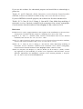
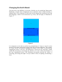
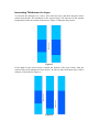
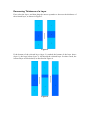
Interactive Receiver Function Forward Modeller
(IRFFM v1.1)
Hrvoje Tkalčić1 and Debdeep Banerjee2
Research School of Earth Sciences
The Australian National University
Canberra, Australia
November 2010
All rights reserved.
General Information & User Manual
1
Research School of Earth Sciences, The Australian National University
e-mail: [email protected] | tel. +061 (0)2 6125 3213
www: http://rses.anu.edu.au/~hrvoje/
2
CSL/RSISE/NICTA, The Australian National University
e-mail: [email protected]
A note to IRFFM users
The Interactive Receiver Function Forward Modeller (IRFFM) is a Java program
written during 2008 for interactive forward modelling of receiver functions (v1.0).
IRFFM v1.1 is the current version and has been available since November 2010.
What is new in v1.1 version?
The new version has been recompiled so that it is compatible with earlier Java
versions (from v1.4 inclusive). It works on 32-bit computers. We have added several
functionalities, most notably: i) the program now comes with a display indicating the
goodness of fit (variance reduction in percentages); ii) an option to print the resulting
plots to either a printer or a jpg file.
What is IRFFM?
IRFFM is a useful complement to the inversion or a stand-alone tool. An easy-to-use
graphic interface is designed to enable the user to efficiently manipulate with
thicknesses and velocities, as well as Vp/Vs ratios in a 1-D model of the earth. It
quickly calculates and displays the theoretical receiver functions and compares them
to the observed receiver functions. It is revealed how the 1-D model has to be
changed to reduce the misfit between the observed and the theoretical waveforms.
Input receiver function is in a two-column ascii format, and the package comes with
an example. Input velocity models are also in ascii format, and two starting models
are provided (ak135 and PREM). The users can use one of these two models as a
starting model, construct their own from other geophysical constraints, or simply
guess the initial earth structure. We typically start with the resulting model from a
grid search (Tkalčić et al. 2006; 2010) with 3 or 4 layers in the crust and 1 layer in
the mantle. It is possible to save current model at any time during the forward
modelling for the future use, or upload a new observed receiver function at any time.
Requirements and assumptions
The method used in IRFFM for the calculation of the theoretical radial receiver
functions utilizes a synthetic seismogram algorithm by G. Randall (respknt), based on
the method developed by Kennett (1983), and a time domain deconvolution to
produce synthetic receiver functions in the same manner as it is done for the observed
receiver functions (iterdecon). Therefore, the program is closely tied to the time
domain iterative deconvolution procedure described by Ligorría and Ammon (1999),
(see C. J. Ammon website http://eqseis.geosc.psu.edu/~cammon/).
In practice, this means that that the user has to make sure that respknt and
iterdecon (both Fortran programs) are installed, compiled and running
independently of IRFFM prior to launching IRFFM.
The main assumptions/lilmitations are that the Earth is parameterized in terms of
homogeneous horizontal layers. While these assumptions are OK in many cases, the
Earth has a more complex structure and the assumptions might not always be valid.
Also, it is assumed that the Earth beneath the receiver is purely isotropic.
Currently available Gaussian filters are a=1.0, 2.5, 5.0 and 10.0.
IRFFM is free software, but it is work in progress and we welcome and encourage
your feedback. Enquiries and feedback can be sent to [email protected].
If you use this software for educational purposes and would like to acknowledge it,
please cite:
Tkalčić, H., and D. Banerjed, (2009), Interactive receiver-function forward modeler
(IRFFM); software and manual available at http://www.rses.anu.edu.au/~hrvoje.
If you use IRFFM in scientific purposes, the software has first been introduced in:
Tkalčić, H., Y. Chen, R. Liu, Z. Huang, L. Sun and W. Chan, Multi-Step modeling of
teleseismic receiver functions combined with constraints from seismic tomography:
Crustal structure beneath southeast China, Geophys. J. Int., submitted, 2010.
References
Kennett, B.L.N. (1983), Approximations to the response of the stratification, in Seismic Wave
Propagation in Stratified Media, chapter 9, Cambridge Univ. Press, New York.
Ligorría, J. P., and C. J. Ammon (1999), Iterative deconvolution and receiver function
estimation, Bull. Seismol. Soc. Am., 89, 1395 – 1400.
Tkalčić, H., and D. Banerjed, (2009), Interactive receiver-function forward modeler (IRFFM);
software and manual available at http://www.rses.anu.edu.au/~hrvoje.
Tkalčić, H., Y. Chen, R. Liu, Z. Huang, L. Sun and W. Chan, Multi-Step modeling of
teleseismic receiver functions combined with constraints from seismic tomography:
Crustal structure beneath southeast China, Geophys. J. Int., submitted, 2010.
Tkalčić, H., Pasyanos, M., Rodgers, A., Gök, R., Walter, W. & Al-Amri, A. (2006), A multistep approach in joint modeling of surface wave dispersion and teleseismic receiver
functions: Implications for lithospheric structure of the Arabian peninsula, J. Geophys.
Res. 111, B11311, doi:10.1029/2005JB004130.
Introduction
This document describes the functionalities of the IRFFM user interface. The IRFFM
helps constructing one-dimensional model of the earth that reduces the misfit between
the synthetic and observed receiver functions.
Figure 1: Screen Shot of IRFFM v1.1
The user interface, as shown in Figure 1, consists of three main parts:
1. The model display section (left side of Figure 1)
2. The receiver function display section (upper right section of Figure 1)
3. The control panel (bottom right section of Figure 1)
The Model Display
The earth model is displayed on the left-hand side of the main window. The model
display consists of two columns; the left one representing the shear wave speed (Vs)
and the right one representing the ratio of compressional and shear wave speeds
(Vp/Vs). The y-axis of each of these columns shows the depth in kilometres. Each
column is divided into layers of varying thicknesses so that the parameters of the
model are layer thickness, Vs speed, and the Vp/Vs ratio. The procedure for changing
these parameters is described in the sections that follow. Only the layers within the
first 220 kilometres are displayed. The default starting model is the ak135 model (the
file called ak135.mod), which can be modified or replaced later.
The IRFFM Display
The observed and the synthetic RFs are displayed at the right hand corner of the main
window. The thick grey line represents the observed RF and the thin yellow line
represents the synthetic RF, calculated from the current model displayed on the left
hand side of the screen. The default observed RF is read from a file called
“example_observed.sac.asc''.
The Control Panel
The control panel provides the buttons and input fields that enable the user to load
different model files and observed RF files, manipulate a model by changing the
parameters of the layers, delete a layer, split a layer in two, control the mouse
movement over the layers, execute the program that generates the synthetic RF from
the model data, etc. A detailed description of the control panel functionality will be
given in the last section.
Changing the Earth Model
The main aim of the IRFFM is to provide a flexible way for modifying Earth model.
Modifying a model means changing the layer parameters and or simply deleting or
splitting layers. The parameters of each layer can be changed by selecting a layer and
then dragging a mouse in four directions: up, down, left and right, as illustrated in
Figure 2.
Figure 2
It is important to note that to perform any manipulation of a layer we need to select
the layer first (when selected, the colour of the layer will turn dark blue). The velocity
of a layer can be increased by dragging the mouse to the right, or decreased by
dragging the mouse to the left. The thicknesses of the layers are associative, which
means that increasing or decreasing the thickness of a layer effects the thickness of
the layer immediately below. The following sub-sections describe the effects of
increasing, decreasing the depth of a layer and the effects of splitting and deleting a
layer.
Increasing Thickness of a Layer
To increase the thickness of a layer, first select the layer and then drag the mouse
pointer downwards. The thickness of the selected layer will increase by the amount
proportional to the movement of the mouse. Figure 3 illustrates the process.
Figure 3
If the depth of the selected layer reached the bottom of the layer below, then the
selected layer will subsume the layer below. In other words, the bottom layer will be
deleted, as described in Figure 4.
Figure 4
Decreasing Thickness of a Layer
First select the layer, and then drag the mouse upwards to decrease the thickness of
the selected layer, as shown in Figure 5.
Figure 5
If the bottom of the selected layer (layer 2) reached the bottom of the layer above
(layer 1), the layer below (layer 3) will absorb the selected layer. In other words, the
selected layer will be deleted, as described in Figure 6.
Figure 6
“Splitting” Layers
There are two ways to divide a layer: 1) splitting a layer by half, and 2) dividing a
layer at a desired point.
1. Select a layer and press “Split Layer” button from the control panel. This will
split the current selected layer into two equal depth layers and the upper half
will be selected. This is illustrated in Figure 7.
Figure 7
2. Specify a position in km from where the selected layer will be split in the field
``Splitting Point'', and then press the “Split Layer'” button in the control panel.
The result of this operation is illustrated in Figure 8.
Figure 8
Deleting Layers
To delete a layer, select the layer to delete and then press the ”Delete Layer'' button in
the control panel. This is illustrated in Figure 9.
Figure 9
The Control Panel
The functions that can be performed from the control panel are described below.
Model Management
The current model file name is displayed in red.





To change the starting synthetic model, press the ”Change Starting Model''
button, and select a new model file. The corresponding synthetic receiver
function will be recalculated.
To save the current model, press “Save Current Model'' button.
To change the parameters of a selected layer, input the new thickness, Vs
speed and Vp/Vs ratio into the corresponding input fields and press the
“Apply'' button.
To split the selected layer, put the depth point form where you want to split
the layer and then press “Split Layer'' button.
To delete the selected layer, press the “Delete Layer'' button.
Receiver Function Management
The current receiver function file name and the slowness in s/km are displayed in red.



To change the observed receiver function, click on the “Change Observed RF''
button and select a new observed receiver function file. After selection, the
display will be updated.
Four different values of the Gaussian parameter can be selected: 1.0, 2.5, 5
and 10. To change the Gaussian parameter, select one of the parameters and
press the “Run'' button in Controls. At the start, 1.0 is default value of the
Gaussian parameter. Match the value of the Gaussian parameter with the value
you used to calculate the observed receiver function.
To change the slowness, press the “Change Slowness'' button and select a
value. Then press the “Run'' button in Controls. At the start, the default value
is 0.065 s/km. Match the value of the slowness with your best estimate for the
slowness of the observed receiver function.
Mouse Movement Control



Horizontal: The effect of mouse dragging is limited to the x-axis. This means
that only the velocity of a layer can be changed by dragging the mouse to the
left or right. This is the default setting.
Vertical: The effect of mouse dragging is limited to the y-axis. This means
that only the thickness of the layers can be changed, by dragging the mouse up
or down.
Any: This option does not limit the effects of mouse-dragging, and both the
thicknesses and the velocities of the selected layers can be changed
simultaneously. This is often less convenient than it looks.
Controls






Run: When the ``Run'' button is pressed, a script is called and the output is
written in the file “outmodel.slowness-param.filter-value.eqr.asc''. For
example, if the slowness is 0.065 s/km, and the Gaussian parameter is 1.0,
then the theoretical RFs file name will be outmodel.0.065.1.0.eqr.asc. This file
will first be generated and then read and displayed in the display section.
Reset: Resets everything to the starting points with their default values.
Print to File: Prints a post-script image file with the model and RF display
Print to Printer: Prints Earth model and RF display via selected printer. User
should choose Landscape mode of printing to get desired print.
Quit: Quits the application.
IRFFM Manual: Information about the IRFFM program.