Download LOQO User`s Manual – Version 4.05

LOQO User’s Manual – Version 4.05
Robert J. Vanderbei
Operations Research and Financial Engineering
Technical Report No. ORFE-99-??
September 13, 2006
Princeton University
School of Engineering and Applied Science
Department of Operations Research and Financial Engineering
Princeton, New Jersey 08544
LOQO USER’S MANUAL – VERSION 4.05
ROBERT J. VANDERBEI
A BSTRACT. LOQO is a system for solving smooth constrained optimization problems. The problems can be linear or nonlinear, convex or nonconvex, constrained or unconstrained. The only real restriction is that the functions defining the problem
be smooth (at the points evaluated by the algorithm). If the problem is convex, LOQO finds a globally optimal solution.
Otherwise, it finds a locally optimal solution near to a given starting point. This manual describes
(1) how to install LOQO on your hardware,
(2) how to use AMPL together with LOQO to solve general convex optimization problems,
(3) how to use the subroutine library to formulate and solve convex optimization problems, and
(4) how to formulate and solve linear and quadratic programs in MPS format.
1. I NTRODUCTION
LOQO
is a system for solving smooth constrained optimization problems in the following form:
minimize
subject to
f (x)
a ≤h(x)≤ b
l ≤ x ≤ u.
Here, the variable x takes values in Rn , l and u are given n-vectors, f is a real-valued function defined on {x : l ≤
x ≤ u}, h is a map from this set into Rm , and a and b are given m-vectors. Some or all components of a and l can
be −∞, whereas some or all components of b and u can be ∞. The functions f and h must be twice differentiable
at the points at which they are evaluated by LOQO. The problem is convex if f is convex, each component function
hi is convex, and ai = −∞ whenever hi is not linear. If the problem is convex, then LOQO finds a globally optimal
solution. Otherwise, it finds a locally optimal solution near to a given starting point.
LOQO is based on an infeasible, primal-dual, interior-point method applied to a sequence of quadratic approximations to the given problem. See [6], [7], and [5] for a detailed discussion of the algorithm implemented in LOQO.
There are three ways to convey problems to LOQO.
(1) For general optimization problems, the prefered user interface is via the AMPL [2] modeling language.
(2) For those without access to AMPL, there is a subroutine library that one can link to their own programs. This
is a painful way to use LOQO, but for some it may be the only option.
(3) If the problem is a linear program, one can use industry standard MPS files as input. If the problem is a
linearly constrained quadratic program, one can use a simple extension of the MPS format. MPS files can be
created either with a specifically created generator program or via any of the popular optimization modeling
languages such as AMPL or GAMS [1].
This manual describes
(1)
(2)
(3)
(4)
how to install LOQO on your hardware,
how to use AMPL together with LOQO to solve general convex optimization problems,
how to use the subroutine library to formulate and solve convex optimization problems, and
how to formulate and solve linear and quadratic programs in MPS format.
Research supported by ONR through grant N00014-98-1-0036 and by NSF through grant CCR-9403789.
1
2
ROBERT J. VANDERBEI
2. I NSTALLATION
The normal mechanism for distribution is by downloading from the author’s homepage:
http://www.princeton.edu/˜rvdb/
Under the heading LOQO Info one can click on Download and follow the instructions on the download web page.
After downloading and unzipping, you will find several files:
An executable code, which can read problems formulated by the AMPL modeling language. For linear programming problems, it can also read industry-standard MPS form
(see afiro.mps for an example) and for quadratic programming problems it can read an
extension of MPS form.
loqo.lib An archive file containing the LOQO function library.
loqo.c
A file containing the main program for loqo. It is included as an example on how to use
the LOQO function library.
hs046.c
A modification of loqo.c illustrating how to use the function library to solve problem 46
in the Hock and Schittkowski [3] test suite.
loqo.h
A header file containing the function prototypes for each function in the LOQO function
library. This file must be #include’d in any program file in which calls to the LOQO
function library are made (loqo.c and hs046.c are examples of this).
myalloc.h A header file containing macros to make dynamic memory allocation less of a chore.
loqo.exe
3. U SING LOQO WITH AMPL
It is easy to use LOQO with AMPL. In an AMPL model one simply puts
option solver loqo;
before the solve command. If one wishes to adjust some user-settable parameters, they can be set within the AMPL
model as well. For example, to increase the amount of output produced by the solver and to request a report of the
solution time, one puts the following statement in the AMPL model ahead of the call to the solver:
option loqo_options "verbose=2 timing=1";
Parameters, their meanings and their defaults, are described in a later section. Hundreds of sample AMPL models can
be downloaded from the author’s homepage http://www.princeton.edu/˜rvdb/. One example is discussed
in the following subsection.
Below we describe one specific real-world model and show how to solve it with AMPL/LOQO.
3.1. The Markowitz Model. Markowitz received the 1990 Nobel Prize in Economics for his portfolio optimization
model in which the tradeoff between risk and reward is explicitly treated. We shall briefly describe this model in its
simplest form. Given a collection of potential investments (indexed, say, from 1 to n), let Rj denote the return in the
next time period on investment j, j = 1, . . . , n. In general, Rj is a random variable, although some investments may
be essentially deterministic.
A portfolio is determined by specifying what fraction of one’s assets to put into each investment. That is, a portfolio
is a collection of nonnegative numbers xj , j = 1, . . . , n that sum to one. The return (on each dollar) one would obtain
using a given portfolio is given by
X
R=
xj Rj .
j
The reward associated with such a portfolio is defined as the expected return:
X
ER =
xj ERj .
j
LOQO USER’S MANUAL – VERSION 4.05
3
Similarly, the risk is defined as the variance of the return:
= E(R − ER)2
X
= E(
xj (Rj − ERj ))2
Var(R)
j
X
= E(
xj R̃j )2 ,
j
where R̃j = Rj − ERj . One would like to maximize the reward while minimizing the risk. In the Markowitz model,
one forms a linear combination of the mean and the variance (parametrized here by µ) and minimizes that:
P
P
maximize
x ERj − µE( j xj R̃j )2
Pj j
subject to
j xj = 1
xj ≥ 0 j = 1, 2, . . . , n.
Here, µ is a positive parameter that represents the importance of risk relative to reward. That is, high values of µ will
tend to minimize risk at the expense of reward whereas low values put more weight on reward.
Of course, the distribution of the Rj ’s is not known theoretically but is arrived at empirically by looking at historical
data. Hence, if Rj (t) denotes the return on investment j at time t (in the past) and these values are known for all j and
for t = 1, 2, . . . , T , then expectations can be replaced by sample means as follows:
ERj =
T
1X
Rj (t).
T t=1
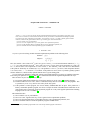
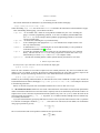
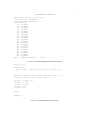
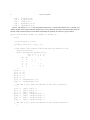
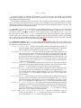
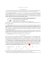
The full model, expressed in AMPL is shown in Figure 1. If we suppose that this model is stored in a file called
markowitz.mod, then the model can be solved by typing:
ampl markowitz.mod
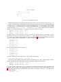
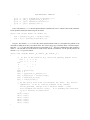
The output that is produced is shown in Figure 2.
4. T HE F UNCTION L IBRARY
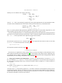
The easiest way to explain how to use the function library is to look at an example. For this discussion we have
chosen problem 46 from the Hock and Schittkowski [3] set of test problems. This problem is fairly small having only
two constraints and five variables. Nonetheless it illustrates most of what one faces when solving problems with the
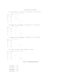
function library. An AMPL listing of the problem is shown in Figure 3.
4.1. Setting Up the Problem in the Calling Routine. To use the LOQO subroutine library, one needs to #include
the LOQO header file loqo.h (and math.h if sines, cosines, exponentials, etc. are to be used). Then, at the place in
the code where the subroutine library is to be accessed, one needs to declare a variable, say lp, that is a pointer to a
LOQO structure:
LOQO *lp;
The variable lp is set to point to a LOQO structure with a call to openlp():
lp = openlp();
After this call, the LOQO data structure pointed to by lp has fields to contain all of the information needed to describe
an optimization problem. However, the fields are set to zero, except for some of the parameters whose defaults have
nonzero values. We must now load up lp with a description of the problem we wish to solve. We begin by specifying
the dimensions and number of nonzeros in the matrices:
4
ROBERT J. VANDERBEI
param n integer > 0 default 500; # number of investment opportunities
param T integer > 0 default 20; # number of historical samples
param mu default 1.0;
param R {1..T,1..n} := Uniform01(); # return for each asset at each time
# (in lieu of actual data,
# we use a random number generator).
param mean {j in 1..n}
# mean return for each asset
:= ( sum{i in 1..T} R[i,j] ) / T;
param Rtilde {i in 1..T,j in 1..n}
:= R[i,j] - mean[j];
# returns adjusted for their means
var x{1..n} >= 0;
minimize linear_combination:
mu *
sum{i in 1..T} (sum{j in 1..n} Rtilde[i,j]*x[j])ˆ2
sum{j in 1..n} mean[j]*x[j]
;
# weight
# variance
# mean
subject to total_mass:
sum{j in 1..n} x[j] = 1;
option solver loqo;
solve;
printf: "Optimal Portfolio: \n";
printf {j in 1..n: x[j]>0.001}: "
%3d %10.7f \n", j, x[j];
printf: "Mean = %10.7f, Variance = %10.5f \n",
sum{j in 1..n} mean[j]*x[j],
sum{i in 1..T} (sum{j in 1..n} Rtilde[i,j]*x[j])ˆ2;
F IGURE 1. The Markowitz model in AMPL.
lp->n = 5;
lp->m = 2;
lp->nz = 6;
lp->qnz = 13;
/* number of variables
(indexed 0,1,...,n-1) */
/* number of constraints (indexed 0,1,...,m-1) */
/* number of nonzeros in linearized constraint matrix */
/* number of nonzeros in Hessian (details below) */
The meaning of nz and qnz, if not clear now, will become clear shortly.
As described in [7], LOQO solves nonlinear optimization problems by forming successive quadratic approximations
to the given problem. The data defining the quadratic approximation will be changed at each iteration. Later we will
define subroutines to do that. First, however, we must allocate storage for the data arrays and we must set up the
sparse representation of the matrices. We begin by allocating storage. The standard dynamic memory allocation
routines, malloc(), realloc(), etc., are fairly clumsy to use. So, we prefer to #include the macro package
myalloc.h to provide memory allocation macros making the code more readable.
LOQO USER’S MANUAL – VERSION 4.05
LOQO: optimal solution (27 iterations)
primal objective -0.6442429719
dual objective -0.6442429757
Optimal Portfolio:
55 0.0947940
110 0.0065178
117 0.0798030
133 0.0939987
139 0.0019013
149 0.0659393
151 0.1004998
204 0.0010385
222 0.0655395
240 0.0659596
302 0.0065309
311 0.0075337
392 0.1939488
414 0.0533825
423 0.0087270
428 0.0212861
444 0.0551152
465 0.0128579
496 0.0385579
497 0.0260684
Mean = 0.6489705, Variance =
0.00473
F IGURE 2. The output produced for the Markowitz model.
var x {1..5};
minimize obj:
(x[1]-x[2])ˆ2 + (x[3]-1)ˆ2 + (x[4]-1)ˆ4 + (x[5]-1)ˆ6
;
subject to constr1: x[1]ˆ2*x[4] + sin(x[4] - x[5]) = 1;
subject to constr2: x[2] + x[3]ˆ4*x[4]ˆ2 = 2;
let
let
let
let
let
x[1]
x[2]
x[3]
x[4]
x[5]
:=
:=
:=
:=
:=
sqrt(2)/2;
1.75;
0.5;
2;
2;
solve;
display x;
F IGURE 3. Hock and Schittkowski 46 in AMPL.
5
6
ROBERT J. VANDERBEI
(var
col
row
0
1
1
0
2
1
3
2
4
3
5)
4
*
*
*
*
*
*
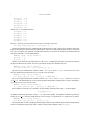
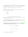
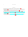
F IGURE 4. The sparsity pattern for A
The matrix containing the linearized part of the constraints is called A. It is stored sparsely in three arrays: A, iA,
kA. Array A contains the values of the nonzeros listed one column after another. This array is a one-dimensional array
of length nz. Array iA contains the row index of each corresponding value in A. It too has length nz, but it contains
ints instead of doubles. The third array, kA, contains a list of indices in the A/iA array indicating where each new
column starts. Hence, kA[0] = 0, kA[n] = nz, and kA[j+1]-kA[j] is the number of nonzero elements in
column j (i.e., associated with variable j). To allocate storage for these arrays, we write:
MALLOC( lp->A, lp->nz, double );
MALLOC( lp->iA, lp->nz, int );
MALLOC( lp->kA, lp->n+1, int );
The data stored in A will be given later. For now we just store the sparsity structure by initializing iA and kA
appropriately. Since the first constraint involves variables x1 , x4 , and x5 and the second constraint involves variables
x2 , x3 , and x4 , we see that the sparsity pattern for A is as shown in Figure 4. Since the data elements are listed in iA
columnwise starting with the zeroeth column, we see that iA needs to be initialized as follows:
lp->iA[0] = 0;
lp->iA[1] = 1;
lp->iA[2] = 1;
lp->iA[3] = 0;
lp->iA[4] = 1;
lp->iA[5] = 0;
Also, the array kA now must be set as follows:
lp->kA[0] = 0;
lp->kA[1] = 1;
lp->kA[2] = 2;
lp->kA[3] = 3;
lp->kA[4] = 5;
lp->kA[5] = 6;
The array A will be given correct values later. For now, we just fill it with zeros:
for (k=0; k<lp->nz; k++) { lp->A[k] = 0; }
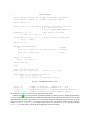
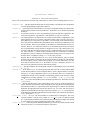
The matrix Q in the quadratic approximation must also be initialized. It is a sparse symmetric matrix. It too is
stored in the usual three-array sparse format. We begin by allocating storage for the three arrays:
MALLOC( lp->Q, lp->qnz, double );
MALLOC( lp->iQ, lp->qnz, int );
MALLOC( lp->kQ, lp->n+1, int );
The matrix Q will be defined later as a linear combination of the Hessian of the objective function and each of the
constraints. Hence, the sparse data structure must contain places for nonzeros from any of these functions. Figure
5 shows the sparsity patterns for each individual function and for the matrix Q. The array iQ must therefore be
initialized as follows:
lp->iQ[0] = 0;
LOQO USER’S MANUAL – VERSION 4.05
For the objective function, the pattern is as follows:
(var 1 2 3 4 5)
col 0 1 2 3 4
var row
1
0
* *
2
1
* *
3
2
*
4
3
*
5
4
*
For the first constraint, the pattern is as follows:
(var 1 2 3 4 5)
col 0 1 2 3 4
var row
1
0
*
*
2
1
3
2
4
3
*
* *
5
4
* *
For the second constraint, the pattern is as follows:
(var 1 2 3 4 5)
col 0 1 2 3 4
var row
1
0
2
1
3
2
* *
4
3
* *
5
4
The union
(var
col 0 1 2
var row
1
0
2
1
3
2
4
3
5
4
of these three patterns is this:
1 2 3 4 5)
3 4
*
*
*
*
*
*
*
*
*
*
*
*
*
F IGURE 5. The sparsity pattern for Q
lp->iQ[1]
lp->iQ[2]
lp->iQ[3]
lp->iQ[4]
lp->iQ[5]
lp->iQ[6]
=
=
=
=
=
=
1;
3;
0;
1;
2;
3;
7
8
ROBERT J. VANDERBEI
lp->iQ[7]
lp->iQ[8]
lp->iQ[9]
lp->iQ[10]
lp->iQ[11]
lp->iQ[12]
=
=
=
=
=
=
0;
2;
3;
4;
3;
4;
And the array kQ is initialized like this:
lp->kQ[0]
lp->kQ[1]
lp->kQ[2]
lp->kQ[3]
lp->kQ[4]
lp->kQ[5]
=
=
=
=
=
=
0;
3;
5;
7;
11;
13;
The array Q will be given correct values later. For now, we just fill it with zeros:
for (k=0; k<lp->qnz; k++) { lp->Q[k] = 0; }
Now that the matrices have been initialized much of the hard work is done. Still we need to initialize some other
things, the first and most obvious being the right-hand side. Since the so-called right-hand side is always assumed to
be a vector of constants (any functions, no matter what side they are written on are assumed to be absorbed into the
body of the constraint), it can be initialized here:
MALLOC( lp->b, lp->m, double );
lp->b[0] = 1;
lp->b[1] = 2;
Another vector that needs space allocated for it is the vector c containing the linear part of the objective function.
The data it contains will be set later. For now we just allocate storage for it and fill it with zeros:
MALLOC( lp->c, lp->n, double );
for (j=0; j<lp->n;
j++) { lp->c[j] = 0; }
The vector of lower bounds on the variables is called l. If l==NULL, then solvelp() will set it to a zero vector.
Since the variables in this problem are free, we reset this vector as follows:
MALLOC( lp->l, lp->n, double );
for (j=0; j<lp->n; j++) { lp->l[j] = -HUGE_VAL; }
The vector of upper bounds on the variables is called u. If u==NULL, then solvelp() will set it to a vector of
HUGE VAL’s. This default behavior is correct for the problem at hand and so nothing needs to be done. Nonetheless,
we set it here so one can see how it is done.
MALLOC( lp->u, lp->n, double );
for (j=0; j<lp->n; j++) { lp->u[j] =
HUGE_VAL; }
Each constraint, such as the i-th, is assumed to be an inequality constraint with a range, ri , on the inequality:
bi ≤ ai (x) ≤ bi + ri .
An equality constraint is specified by setting r[i] to 0 (this is the default). An inequality constraint is specified by
setting it to HUGE VAL. Since the default behavior is easy to forget, it is a good idea to set r explicitly as we do here.
MALLOC( lp->r, lp->m, double );
for (i=0; i<lp->m; i++) { lp->r[i] = 0; }
The functions that are used to update the quadratic approximation to the nonlinear problem will be defined shortly.
To make sure that these functions get called, we must set some pointers and put a call to nlsetup():
LOQO USER’S MANUAL – VERSION 4.05
9
lp->objval = objval;
lp->objgrad = objgrad;
lp->hessian = hessian;
lp->conval = conval;
lp->congrad = congrad;
nlsetup( lp );
The solver, which will be called shortly, is happy to compute its own default starting point and without further
action will do just that. However, for the problem at hand a specific starting point was given. To force the solver to
use that point, we include the following lines:
MALLOC( lp->x, lp->n, double );
lp->x[0] = sqrt(2.)/2;
lp->x[1] = 1.75;
lp->x[2] = 0.5;
lp->x[3] = 2;
lp->x[4] = 2;
Finally, before calling the solver we can set a number of parameters that control the algorithm. A complete list of
them can be found in loqo.h. One of them is called verbose. It is an integer variable. The higher the value, the
more output produced during the solution process. The default value is zero (no output). Here we set it higher.
lp->verbose = 2;
We are now ready to put the call to the solver in the calling routine:
solvelp( lp );
The function solvelp() returns an integer that indicates whether or not the algorithm was successful (zero means
success, positive means failure). The return value can be ignored by simply not assigning it to anything as is done
above.
After the solver returns, one might wish to print out the solution vector and the solution time. Here is the code to
do that:
if (lp->verbose>1) {
printf("x: \n");
for (j=0; j<lp->n; j++) {
printf("%2d %12.6f \n", j+1, lp->x[j]);
}
printf("total time in seconds = %lf \n", cputimer() );
}
4.2. Updating the Quadratic Approximation. Certain specific functions must be provided that tell how to compute
the quadratic approximation to the problem. We describe these functions here.
Objval. The function objval takes x as input and returns the objective function value. For the problem at hand,
this function is given as follows:
static double objval( double *x )
{
return pow(x[0]-x[1],2) + pow(x[2]-1,2) + pow(x[3]-1,4) + pow(x[4]-1,6);
}
Note that the function pow() is part of the math library that is standard in ANSI C.
Objgrad. The function objgrad takes x as input and puts the gradient of the objective function at x into array c.
For the Hock and Schittkowski problem, this function is given as follows:
10
ROBERT J. VANDERBEI
c[0]
c[1]
c[2]
c[3]
c[4]
= 2*(x[0]-x[1]);
= -2*(x[0]-x[1]);
= 2*(x[2]-1);
= 4*pow(x[3]-1,3);
= 6*pow(x[4]-1,5);
Hessian. The function hessian takes the primal-variables array x and the dual-variables array y and fills in Q
with the Hessian of the objective function minus the sum over the nonlinear constraints of the dual variable times the
Hessian of that constraint function. For the Hock and Schittkowski problem, this function is given as follows:
static void hessian( double *Q, double *x, double *y )
{
int k;
/* Initialize Q[] to zero
*/
for (k=0; k<13; k++) { Q[k] = 0; }
/* Now feed in the nonzeros associated with the Hessian of the
objective function.
Recall the sparsity pattern for Q:
(var 1 2 3 4 5)
col 0 1 2 3 4
var row
1
0
* *
*
2
1
* *
3
2
* *
4
3
*
* * *
5
4
* *
*/
Q[ 0] += 2;
Q[ 1] += -2;
Q[ 3] += -2;
Q[ 4] += 2;
Q[ 5] += 2;
Q[ 9] += 4*3*pow(x[3]-1,2);
Q[12] += 6*5*pow(x[4]-1,4);
/* Now add in y[0] times the Hessian of the first constraint
*/
Q[ 0] -= y[0]*( 2*x[3] );
Q[ 2] -= y[0]*( 2*x[0] );
Q[ 7] -= y[0]*( 2*x[0] );
Q[ 9] -= y[0]*( -sin(x[3]-x[4]) );
Q[10] -= y[0]*( sin(x[3]-x[4]) );
Q[11] -= y[0]*( sin(x[3]-x[4]) );
Q[12] -= y[0]*( -sin(x[3]-x[4]) );
/* Now add in y[1] times the Hessian of the second constraint
*/
LOQO USER’S MANUAL – VERSION 4.05
Q[
Q[
Q[
Q[
5]
6]
8]
9]
-=
-=
-=
-=
y[1]*(
y[1]*(
y[1]*(
y[1]*(
11
4*3*pow(x[2],2)*pow(x[3],2) );
4*pow(x[2],3)*2*x[3] );
4*pow(x[2],3)*2*x[3] );
pow(x[2],4)*2 );
}
Conval. The function conval takes the primal solution x and fills in the vector h with the values of the constraints.
For the problem at hand, this function is given as follows:
static void conval( double *h, double *x )
{
h[0] = pow(x[0],2)*x[3] + sin(x[3]-x[4]);
h[1] = x[1] + pow(x[2],4)*pow(x[3],2);
}
Congrad. The function congrad takes the current primal solution stored in x and updates the gradient of the
constraints by filling in the array A described earlier. The solver keeps a copy of both the matrix A and its transpose.
Therefore, congrad must also update the sparse representation of AT . The array containing these data elements is
called At. One can think of it as the matrix A stored rowwise instead of columnwise. For the specific problem, the
function congrad is given as follows:
static void congrad( double *A, double *At, double *x )
{
/* To fill in the values of A[], recall the sparsity pattern for A:
(var 1 2 3 4 5)
col 0 1 2 3 4
row
0
*
* *
1
* * *
*/
A[0] = 2*x[0]*x[3];
A[1] = 1;
A[2] = 4*pow(x[2],3)*pow(x[3],2);
A[3] = pow(x[0],2) + cos(x[3]-x[4]);
A[4] = 2*pow(x[2],4)*x[3];
A[5] = -cos(x[3]-x[4]);
/* At this point, both A and its transpose, At, exist. At[] must be
updated too. To do it, read the elements of A[] rowwise.
For big problems, libloqo.a has a function atnum(...) that
will recompute the entries of At[]. It is probably more efficient
to do it directly as shown below.
*/
At[0] = A[0];
At[1] = A[3];
At[2] = A[5];
At[3] = A[1];
At[4] = A[2];
At[5] = A[4];
}
12
ROBERT J. VANDERBEI
4.3. Compiling and Running. We have now described all of the pieces necessary to solve the Hock and Schittkowski
problem using the LOQO subroutine library. The complete source is included with the software distribution as file
hs046.c.
All that remains is to show how to compile and execute. These last two tasks are particularly easy:
cc hs046.c libloqo.a -lm -o hs046
hs046
If all goes well, the solver should print out an iteration log showing that it solves the problem in 20 iterations. The
optimal solution is printed out at the end. It should be:
x:
1
2
3
4
5
1.003823
1.003823
1.000000
0.998087
1.003820
5. S OLVING L INEAR AND Q UADRATIC P ROGRAMS IN MPS F ORMAT
Solving linear programs that are already encoded in MPS format is easy. For example, to solve the linear program
stored in myfirstlp.mps, you simply type
loqo -m myfirstlp
Loqo displays a banner announcing itself and when done puts the optimal solution (primal, dual and reduced costs)
in a file myfirstlp.out (which is derived from themyfirstlp on the NAME line of myfirstlp.mps). The
solution file can then be perused using any file editor (such as vi or emacs).
5.1. MPS File Format. Input files follow the standard MPS format (for a detailed description, see [4]) for linear
programs and are an extension of this format in the case of quadratic programs. The easiest way to describe the format
is to look at an example. Consider the following quadratic program:
1
minimize 3x1 − 2x2 + x3 − 4x4 + (x3 − 2x4 )2
2
x1
−3x1
x1
x1 free,
+x2
+x2
+x2
+x2
−4x3
−2x3
+2x4
−x4
−x3
− 100 ≤ x2 ≤ 100,
The input file for this quadratic program looks like this:
≥
4
≤
6
= −1
=
0
x3 , x4 ≥ 0.
LOQO USER’S MANUAL – VERSION 4.05
13
1
2
3
4
5
6
123456789012345678901234567890123456789012345678901234567890
NAME
ROWS
G r1
L r2
E r3
E r4
N obj
COLUMNS
x1
x1
x2
x2
x2
x3
x3
x4
x4
RHS
rhs
rhs
BOUNDS
FR
LO
UP
QUADS
x3
x3
x4
ENDATA
myfirstlp
r1
r4
r1
r3
obj
r1
r4
r1
obj
1.
1.
1.
1.
−2.
−4.
−1.
2.
−4.
r2
obj
r2
r4
−3.
3.
1.
1.
r2
obj
r3
−2.
1.
−1.
r1
r3
4.
−1.
r2
6.
x1
x2
x2
−100.
100.
x3
x4
x4
1.
−2.
4.
Upper case labels must be upper case and represent MPS format keywords. Lower case labels could have been upper
or lower case. They represent information particular to this example. Column alignment is important and so a column
counter has been shown across the top (tabs are not allowed).
The ROWS section assigns a name to each row and indicates whether it is a greater than row (G), a less than row
(L), an equality row (E), or a nonconstrained row (N). Nonconstrained rows refer to the linear part of the objective
function.
The COLUMNS section contains column and row label pairs for each nonzero in the constraint matrix together
with the coefficient of the corresponding nonzero element. Note that either one or two nonzeros can be specified on
each line of the file. There is no requirement about whether one or two values are specified on a given line although
the trend is to specify just one nonzero per line (this uses slightly more disk space, but disk storage space is cheap and
the one-per-line format is easier to read). All the nonzeros for a given column must appear together, but the row labels
within that column can appear in any order.
The RHS section is where the values of nonzero right-hand side values are given. The label “rhs” is optional.
14
ROBERT J. VANDERBEI
By default all variables are assumed to be nonnegative. If some variables have other bounds, then a BOUNDS
section must be included. The label FR indicates that a variable is free. The labels LO and UP indicate lower and
upper bounds for the specified variable.
If the problem has quadratic terms in the objective, their coefficients can be specified by including a QUADS
section. The format of the QUADS section is the same as the COLUMNS section except that the labels are columncolumn pairs instead of column-row pairs. Note that only diagonal and below diagonal elements are specified. The
above diagonal elements are filled in automatically.
5.2. Spec Files. LOQO has only a small number of user adjustable parameters. It is easiest to set these parameters
using the shell variable loqo options. But, to maintain compatibility with older versions of LOQO, one can also
set parameter values at the top of the MPS file or in a separate specfile. If the MPS file is myfirstlp.mps,
the specfile must be called myfirstlp.spc. The parameters have default values which are usually appropriate,
but other values can be specified by including in the MPS file appropriate keywords and, if required, corresponding
values. These keywords (and values) must appear one per line and all must appear before the NAME line in the MPS
file. A list of the parameter keywords can be found in Appendix A.
5.3. Termination Conditions. Once loqo starts iterating toward an optimal solution, there are a number of ways
that the iterations can terminate. Here is a list of the termination conditions that can appear at the end of the iteration
log and how they should be interpreted:
OPTIMAL SOLUTION FOUND Indicates that an optimal solution to the optimization problem was
found. The default criteria for optimality are that the primal and dual agree to 8 significant
figures and that the primal and dual are feasible to the 1.0e-6 relative error level.
SUBOPTIMAL SOLUTION FOUND If at some iteration, the primal and the dual problems are feasible and at the next iteration the degree of infeasibility (in either the primal or the dual)
increases significantly, then loqo will decide that numerical instabilities are beginning to
play heavily and will back up to the previous solution and terminate with this message. The
amount of increase in the infeasibility required to trigger this response is tied to the value
of INFTOL2. Hence, if you want to force loqo to go further, simply set this parameter to
a value larger than the default.
ITERATION LIMIT Loqo will only attempt 200 iterations. Experience has shown that if an optimal
solution has not been found within this number of iterations, more iterations will not help.
Typically, loqo solves problems in somewhere between 10 and 60 iterations.
PRIMAL INFEASIBLE If at some iteration, the primal is infeasible, the dual is feasible and at the
next iteration the degree of infeasibility of the primal increases significantly, then loqo
will conclude that the problem is primal infeasible. If you are certain that this is not the
case, you can force loqo to go further by rerunning with INFTOL2 set to a larger value
than the default.
DUAL INFEASIBLE If at some iteration, the primal is feasible, the dual is infeasible and at the next
iteration the degree of infeasibility of the dual increases significantly, then loqo will conclude that the problem is dual infeasible. If you are certain that this is not the case, you can
force loqo to go further by rerunning with INFTOL2 set to a larger value than the default.
PRIMAL and/or DUAL INFEASIBLE If at some iteration, the primal and the dual are infeasible
and at the next iteration the degree of infeasibility in either the primal or the dual increases
significantly, then loqo will conclude that the problem is either primal or dual infeasible.
If you are certain that this is not the case, you can force loqo to go further by rerunning
with INFTOL2 set to a larger value than the default.
PRIMAL INFEASIBLE (INCONSISTENT EQUATIONS) This type of infeasibility is only detected at the first iteration. If loqo terminates here and you are sure that it should go
on, set the parameter EPSSOL to a larger value than its default.
LOQO USER’S MANUAL – VERSION 4.05
15
6. M ODELING H INTS
Every attempt has been made to make LOQO as robust as possible on a wide spectrum of problem instances.
However, there are certain suggestions that the modeler should take heed of to obtain maximum performance.
6.1. Convex Quadratic Programs. In LOQO version 3.10, some parameter values have different defaults depending
on whether a problem is linear or not (see Appendix A for a list of all parameters and their defaults). Consequently,
quadratic programming problems are treated as general nonlinear problems even though the appropriate default values
for linear programming work much better on these problems. Therefore, we recommend the following nondefault
parameter settings when solving convex quadratic programming problems:
• convex: ensures that none of the special code for nonconvex nonlinear programming is called.
• bndpush=100: ensures that initial values are sufficiently far removed from their bounds.
• honor bnds=0: allows variables to violate their bounds initially.
• pred corr=1: enables the predictor-corrector method.
• mufactor=0: sets the predictor direction to the primal-dual affine-scaling direction.
Future releases of LOQO will ensure that these are the defaults for convex quadratic programming problems (as was
the case in earlier releases).
6.2. Artificial Variables. Splitting free variables. Some existing codes for solving linear programs are unable to
handle free variables. As a consequence, many problems have been formulated with free variables split into the
difference between two nonnegative variables. This trick does not present any difficulties for algorithms based on the
simplex method, but it does tend to cause problems for interior-point methods and, in particular, for LOQO. Since
LOQO is designed to be able to handle problems with free variables, we suggest that they be left as free variables and
indicated as such in the input file.
Artificial Big-M Variables. Some problems have artificial variables added to guarantee feasibility using the traditional Big-M method. Putting huge values anywhere in a problem invites numerical problems. LOQO has its own
feasibility phase and so we suggest that any Big-M type artificial variables be left out.
6.3. Separable Equivalents. Many nonlinear functions have the following form:
f (x) = φ(aT x),
where a is a sparse n-vector of coefficients and φ is a convex function. Suppose, for the sake of discussion, that a
involves k nonzeros. Then, the Hessian of f contributes a k × k dense submatrix to the n × n hopefully-sparse matrix
Q of quadratic terms in the quadratic approximation. This might not be bad, but if k is close to n or if there are a lot
of such nonlinear functions, Q might turn out to be quite dense. An alternative is to introduce an artificial variable
y = aT x and replace f (x) by φ(y) together with the linear constraint to define y in terms of x. Since y is a single
real variable, the Hessian now contributes a single diagonal entry to Q. Thus, at the expense of adding a single linear
constraint to the problem, Q is greatly sparsified. This modeling trick can on some problems have a dramatic impact
on efficiency, for example in portfolio optimization problems. In other contexts it doesn’t help, in fact it can hurt.
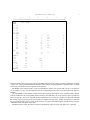
We illustrate this concept with the Markowitz model presented in Section 3.1. By setting the verbosity level to 2,
one discovers the following statistics associated with markowitz.mod:
variables: non-neg
500,
constraints: eq
1,
nonzeros:
A
500,
nonzeros:
L
125750,
free
0,
ineq
0,
Q
250000
arith_ops
bdd
ranged
0,
0,
total
total
500
1
42168001
The second entry on the third line gives the number of nonzeros in the matrix Q defining the quadratic terms. Here it
is 250000 which is exactly 500 squared. This indicates that Q is a dense 500 × 500 matrix.
Now, let us consider a slight modification to the model, which we have stored in a new file called markowitz2.mod:
16
ROBERT J. VANDERBEI
param n integer > 0 default 500; # number of investment opportunities
param T integer > 0 default 20; # number of historical samples
param mu default 1.0;
param R {1..T,1..n} := Uniform01(); # return for each asset at each time
# (in lieu of actual data,
# we use a random number generator).
param mean {j in 1..n}
# mean return for each asset
:= ( sum{i in 1..T} R[i,j] ) / T;
param Rtilde {i in 1..T,j in 1..n}
:= R[i,j] - mean[j];
# returns adjusted for their means
var x{1..n} >= 0;
var y{1..T};
minimize linear_combination:
mu *
sum{i in 1..T} y[i]ˆ2
sum{j in 1..n} mean[j]*x[j]
;
# weight
# variance
# mean
subject to total_mass:
sum{j in 1..n} x[j] = 1;
subject to definitional_constraints {i in 1..T}:
y[i] = sum{j in 1..n} Rtilde[i,j]*x[j];
option solver loqo;
option loqo_options "verbose=2";
solve;
printf: "Optimal Portfolio: \n";
printf {j in 1..n: x[j]>0.001}: "
%3d %10.7f \n", j, x[j];
printf: "Mean = %10.7f, Variance = %10.5f \n",
sum{j in 1..n} mean[j]*x[j],
sum{i in 1..T} (sum{j in 1..n} Rtilde[i,j]*x[j])ˆ2;
If we make a timed run of this model (by typing time ampl markowitz2.mod), the first few lines of output look
like this:
LOQO 3.03: verbose=2
variables: non-neg
500,
constraints: eq
21,
nonzeros:
A
10520,
nonzeros:
L
10730,
free
ineq
Q
arith_ops
20,
0,
20
bdd
ranged
0,
0,
256121
total
total
520
21
LOQO USER’S MANUAL – VERSION 4.05
17
Note that there are now 20 more constraints but at the same time the number of nonzeros in Q is only 20. Furthermore,
the number of arithmetic operations (which correlates closely with true run-times – at least for large problems) is
only 256121 as compared with 42168001 in markowitz.mod. This suggest that the second formulation should run
perhaps a hundred times faster than the first. Indeed, running both models on the same hardware platform one finds
that markowitz2.mod solves in 4.54 seconds whereas markowitz.mod takes 257 seconds, which translates to
a speedup by a factor of about 60. On this problem, MINOS takes 1.25 seconds whereas LANCELOT takes 9.89
seconds.
6.4. Dense Columns. Some problems are naturally formulated with the constraint matrix having a small number of
columns that are significantly denser than the other columns. From an efficiency point of view, dense columns have
been a red herring for interior-point methods. However, LOQO incorporates certain specific techniques to avoid the
inefficiencies often encountered on models with dense columns.
Recently discovered “tricks” (which are incorporated into LOQO) have largely overcome the problems associated
with dense columns, however, the user should be aware that the presense of dense columns could be the source of
numerical difficulties. Often it is easy to reformulate a problem having dense columns in such a way that the new
formulation avoids dense columns. For example, if variable x appears in a large number of constraints, we would
suggest introducing several different variables, x1 , . . . , xk , all representing the same original variable x and using x1
in some of the constraints, x2 in some others, etc. Of course, k − 1 new constraints must be added to equate each of
these new variables to each other. Hence, the new problem will have k − 1 more variables and k − 1 more constraints,
but it will have a constraint matrix that doesn’t have dense columns. Often it is better to solve a slightly larger problem
if the larger constraint matrix has an improved sparsity structure.
18
ROBERT J. VANDERBEI
R EFERENCES
[1] A. Brooke, D. Kendrick, and A. Meeraus. GAMS: A User’s Guide. Scientific Press, 1988. 1
[2] R. Fourer, D.M. Gay, and B.W. Kernighan. AMPL: A Modeling Language for Mathematical Programming. Scientific Press, 1993. 1
[3] W. Hock and K. Schittkowski. Test examples for nonlinear programming codes. Lecture Notes in Economics and
Mathematical Systems 187. Springer Verlag, Berlin-Heidelberg-New York, 1981. 2, 3
[4] J.L. Nazareth. Computer Solutions of Linear Programs. Oxford University Press, Oxford, 1987. 12
[5] D.F. Shanno and R.J. Vanderbei. Interior-Point Methods for Nonconvex Nonlinear Programming: Orderings and
Higher-Order Methods. Math. Prog., 87(2):303–316, 2000. 1
[6] R.J. Vanderbei. LOQO: An interior point code for quadratic programming. Optimization Methods and Software,
12:451–484, 1999. 1
[7] R.J. Vanderbei and D.F. Shanno. An Interior-Point Algorithm for Nonconvex Nonlinear Programming. Computational Optimization and Applications, 13:231–252, 1999. 1, 4
LOQO USER’S MANUAL – VERSION 4.05
A PPENDIX A. A DJUSTABLE PARAMETERS
Here is a list of the parameter keywords with a description of each keyword’s meaning and how to use it:
bndpush value Specifies minimum initial value for slack variables. The default is 100 if the problem
is a linear programming problem and 1 otherwise.
bounds str Specifies the name of the bounds set. Str must be a string that matches one of the boundsset labels in the bounds section of the MPS file. The default is to use the first encountered
bounds set.
convex
Asserts that a problem is convex, thus disabling special treatment that’s appropriate only
for nonconvex problems. The default is to treat problems as if they are nonconvex.
dense n
The ordering heuritics mentioned above are actually implemented as modifications of the
usual heuristics into two-tier versions of the basic heuristic. This is necessary since the reduced KKT system is not positive semi-definite. For each column of the constraint matrix,
there is an associated column in the reduced KKT system. Generally, speaking these are the
tier-one columns. These tier-one columns are intended to be eliminated before the tier-two
columns. However, it is sometimes possible to see tremendous improvements in solution
time if a small number of these columns are assigned to tier-two. The columns whose reassignment could make the biggest impact are those columns which have the most nonzeros
(i.e. dense columns). LOQO has a built in heuristic that tries to determine a reasonable
threshold above which a column will be declared dense and put into tier-two. However, the
heuristic can be overridden by setting dense to any value you want.
dual
Requests that the ordering heuristic be set to favor the dual problem. This is typically
prefered if the number of constraints far exceeds the number of variables or if the problem
has a large number of dense columns. More generally, it is prefered if the matrix AAT has
more nonzeros than the matrix AT A. By default LOQO uses a heuristic to decide if it is
better to use the primal-favored or the dual-favored ordering.
epsdiag eps Specifies minimum value for diagonal elements in reduced KKT system. The default
is 1.0e-14.
epsnum eps At the heart of LOQO is a factorization routine that factors the so-called reduced KKT
system into the product of a lower triangular matrix L times a diagonal matrix D times the
transpose of L. If the reduced KKT system is not of full rank, then a zero will appear on
each diagonal element of D for which the corresponding equation can be written as a linear
combination of preceding equations. epsnum is a tolerance — if Djj ≤ epsnum, then
the j th row of the reduced KKT system is declared a dependent row. The default value for
epsnum is 0.0.
epssol eps Having dependent rows in the reduced KKT system is not by itself an indication of
trouble. All that is required is that when solving the system using the forward and backward
substitution procedures, it is required that when encountering a row that has been declared
dependent, the right-hand side element must also be zero. If it is not, then the system of
equations is inconsistent and a message to this effect is printed. epssol is a zero tolerance
for deciding how small this right-hand side element must be to be considered equivalent to
a zero. The default is 1.0e-6.
honor bnds boolean In LOQO, only slack variables are constrained to be nonnegative. The vector
of primal variables x is always a free variable. If honor bnds is set to 1, then any bounds
on x in the original formulation will be honored when calculating step lengths. The default
is 0 if the problem is a linear programming problem and 1 otherwise.
ignore initsol If an initial primal and/or dual solution is given in an AMPL model, then this initial
solution is passed to LOQO unless this parameter is specified.
19
20
ROBERT J. VANDERBEI
inftol eps
Specifies the infeasibility tolerance for the primal and for the dual problems. The default
is 1.0e-5.
inftol2 eps Specifies the infeasibility tolerance used by the stopping rule to decide if matters are
deteriorating. That is, if the new infeasibility is greater than the old infeasibility by more
than INFTOL2 then stop and declare the problem infeasible. The default is 1.0.
iterlim
Specifies a maximum number of iterations to perform. Generally speaking the an optimal
solution hasn’t been found after about 50 or 60 iterations, it is quite likely that something
is wrong with the model (or with LOQO itself) and it is best to quit. The default is 200.
Requests that only a linear approximation be formed at each iteration.
lp only
max
Requests that the problem be a maximization instead of a minimization. (If calling from
AMPL, the sense of the optimization is specified by AMPL.)
maximize Same as max.
maxit n
Specifies the maximum number of iterations. The default is 200.
min
Requests that the problem be a minimization (this is the default).
mindeg
This keyword requests the minimum degree heuristic (this is the default).
minimize Same as min.
minlocfil This keyword requests the minimum-local-fill heuristic. This heuristic is slower than
the minimum degree heuristic, but sometimes it generates significantly better orderings
yielding an overall win.
mufactor value Specifies a scale factor for the calculation of the centering parameter µ in the predictor step. The default is 0.0 for linear programming problems and 0.1 otherwise.
noreord
The rows and columns of the reduced KKT system are symmetrically permuted using a
heuristic that aims to minimize the amount of fill-in in L. Two heuristics are available:
minimum degree and minimum-local-fill (which is also called minimum-deficiency). If you
wish to use neither of these heuristics and simply solve the system in the original order,
include the noreord keyword.
obj str
Specifies the name of the objective function. Str must be a string that matches one of the N
rows in the rows section of the MPS file. The default is to use the first encountered N row.
outlev n Same as verbose.
pred corr boolean Controls whether or not a corrector direction is computed. Setting to 0 gives a
pure predictor computation, whereas setting to 1 gives a predictor-corrector direction. The
default is 1 for linear programming and 0 otherwise.
primal
Requests that the ordering heuristic be set to favor the primal problem. This is typically
prefered if the number of variables far exceeds the number of constraints or if the problem
has a large number of dense rows. More generally, it is prefered if the matrix AAT has
fewer nonzeros than the matrix AT A. By default LOQO uses a heuristic to decide if it is
better to use the primal-favored or the dual-favored ordering.
ranges str Specifies the name of the range set. Str must be a string that matches one of the range-set
labels in the ranges section of the MPS file. The default is to use the first encountered range
set.
rhs str
Specifies the name of the right-hand side. Str must be a string that matches one of the
right-hand side labels in the right-hand side section of the MPS file. The default is to use
the first encountered right-hand side.
sigfig n Specifies the number of significant figures to which the primal and dual objective function
values must agree for a solution to be declared optimal. The default is 8.
steplen value Step length reduction factor. The default is 0.95.
timing boolean Set to 1 to output timing information and to 0 otherwise. The default is 0.
timlim tmax Sets a maximum time in seconds to let the system run. The default is forever.
LOQO USER’S MANUAL – VERSION 4.05
verbose n
Larger values of n result in more statistical information printed on standard output. Zero
indicates no printing to standard output. The default value is 1.
zero initsol Assert that the primal and dual vectors should be initialized to 0 even if the calling
AMPL model specifies initial values.
21
22
ROBERT J. VANDERBEI
ROBERT J. VANDERBEI , O PERATIONS R ESEARCH AND F INANCIAL E NGINEERING , P RINCETON U NIVERSITY , P RINCETON , NJ 08544
E-mail address: [email protected]