Download Community Sea Ice Model (CSIM) User`s Guide Version 5.0

Community Climate System Model
National Center for Atmospheric Research, Boulder, CO
http://www.ccsm.ucar.edu/models
CVS tag $Name$ Build date: July 12, 2004
Community Sea Ice Model (CSIM) User’s Guide
Version 5.0
Released with CCSM3.0
Julie Schramm
Cecilia Bitz
Bruce Briegleb
Marika Holland
Elizabeth Hunke
Bill Lipscomb
Dick Moritz
Contents
1 Introduction
1.1 What’s new in CSIM5?
. . . . . . . . . . . . . . . . . . . . . . . . . . . . . . . . . . . . . . .
2 Quick Start Guide
2.1 What is needed to run CSIM? . . . . . . . . . .
2.2 Downloading Source Code and Input Datasets .
2.3 Running CSIM Coupled . . . . . . . . . . . . .
2.4 Running CSIM Uncoupled . . . . . . . . . . . .
2.4.1 Multiple Processors with MPI . . . . . .
2.4.2 Single Processor with MPI . . . . . . .
2.4.3 Single Processor without MPI . . . . . .
3 The CSIM Scripts
3.1 Coupled Model Scripts . . . . . . . . . . . .
3.2 Uncoupled Run Script . . . . . . . . . . . .
3.2.1 Using the Ocean Mixed Layer Model
3.2.2 Changing Grid Resolution . . . . . .
3.2.3 Changing the Number of Processors
3.3 Uncoupled Setup Script . . . . . . . . . . .
3.4 The Build Environment . . . . . . . . . . .
3.4.1 CSIM Preprocessor Flags . . . . . .
3.4.2 CSIM Compiler Options . . . . . . .
.
.
.
.
.
.
.
.
.
.
.
.
.
.
.
.
.
.
.
.
.
.
.
.
.
.
.
.
.
.
.
.
.
.
.
.
.
.
.
.
.
.
.
.
.
.
.
.
.
.
.
.
.
.
.
.
.
.
.
.
.
.
.
.
.
.
.
.
.
.
.
.
.
.
.
.
.
.
.
.
.
.
.
.
.
.
.
.
.
.
.
.
.
.
.
.
.
.
.
.
.
.
.
.
.
.
.
.
.
.
.
.
.
.
.
.
.
.
.
.
.
.
.
.
.
.
.
.
.
.
.
.
.
.
.
.
.
.
.
.
.
.
.
.
.
.
.
4
4
5
5
6
7
7
7
. . . .
. . . .
CSIM
. . . .
. . . .
. . . .
. . . .
. . . .
. . . .
.
.
.
.
.
.
.
.
.
.
.
.
.
.
.
.
.
.
.
.
.
.
.
.
.
.
.
.
.
.
.
.
.
.
.
.
.
.
.
.
.
.
.
.
.
.
.
.
.
.
.
.
.
.
.
.
.
.
.
.
.
.
.
.
.
.
.
.
.
.
.
.
.
.
.
.
.
.
.
.
.
.
.
.
.
.
.
.
.
.
.
.
.
.
.
.
.
.
.
.
.
.
.
.
.
.
.
.
.
.
.
.
.
.
.
.
.
.
.
.
.
.
.
.
.
.
.
.
.
.
.
.
.
.
.
.
.
.
.
.
.
.
.
.
.
.
.
.
.
.
.
.
.
.
.
.
.
.
.
.
.
.
.
.
.
.
.
.
.
.
.
.
.
.
.
.
.
.
.
.
7
8
8
8
8
9
9
11
11
12
. . . . . . . . . . . .
. . . . . . . . . . . .
. . . . . . . . . . . .
. . . . . . . . . . . .
. . . . . . . . . . . .
. . . . . . . . . . . .
. . . . . . . . . . . .
. . . . . . . . . . . .
. . . . . . . . . . . .
. . . . . . . . . . . .
. . . . . . . . . . . .
Atmospheric Forcing
. . . . . . . . . . . .
.
.
.
.
.
.
.
.
.
.
.
.
.
.
.
.
.
.
.
.
.
.
.
.
.
.
.
.
.
.
.
.
.
.
.
.
.
.
.
.
.
.
.
.
.
.
.
.
.
.
.
.
.
.
.
.
.
.
.
.
.
.
.
.
.
.
.
.
.
.
.
.
.
.
.
.
.
.
.
.
.
.
.
.
.
.
.
.
.
.
.
.
.
.
.
.
.
.
.
.
.
.
.
.
.
.
.
.
.
.
.
.
.
.
.
.
.
.
.
.
.
.
.
.
.
.
.
.
.
.
.
.
.
.
.
.
.
.
.
.
.
.
.
.
.
.
.
.
.
.
.
.
.
.
.
.
.
.
.
.
.
.
.
.
.
.
.
.
.
.
.
.
.
.
.
.
.
.
.
.
.
.
.
.
.
.
.
.
.
.
.
.
.
.
.
12
12
13
13
13
16
17
18
18
18
19
20
20
21
.
.
.
.
.
.
.
.
.
.
.
.
.
.
. . . .
. . . .
within
. . . .
. . . .
. . . .
. . . .
. . . .
. . . .
4 Namelist Variables
4.1 Changing the Length of the Model Run . . .
4.2 Changing the timestep . . . . . . . . . . . . .
4.3 Writing Output . . . . . . . . . . . . . . . . .
4.4 Model Physics . . . . . . . . . . . . . . . . . .
4.5 File Names . . . . . . . . . . . . . . . . . . .
4.6 Ocean Mixed Layer Model . . . . . . . . . . .
4.7 Atmospheric Forcing . . . . . . . . . . . . . .
4.8 Example Namelists . . . . . . . . . . . . . . .
4.8.1 Example 1: CCSM Fully Coupled . .
4.8.2 Example 2: Coupled Ice Only Model .
4.8.3 Example 3: Uncoupled Ice Model . . .
4.8.4 Example 4: Uncoupled Ice Model with
4.8.5 Example 5: History File Namelist . .
3
3
.
.
.
.
.
.
.
.
.
.
.
.
.
.
.
.
.
.
.
.
.
5 Model Input Datasets
21
5.1 Atmospheric Forcing . . . . . . . . . . . . . . . . . . . . . . . . . . . . . . . . . . . . . . . . . 22
6 Run Types
22
6.1 Startup Runs . . . . . . . . . . . . . . . . . . . . . . . . . . . . . . . . . . . . . . . . . . . . . 22
6.2 Continue Runs . . . . . . . . . . . . . . . . . . . . . . . . . . . . . . . . . . . . . . . . . . . . 23
7 Changing the Number of Ice Thickness Categories
8 Output Data
8.1 Stdout Output . . . . . . . . . . . . . . . .
8.2 Restart Files . . . . . . . . . . . . . . . . .
8.3 History Files . . . . . . . . . . . . . . . . .
8.3.1 Caveats Regarding Averaged Fields
8.3.2 Changing Frequency and Averaging
.
.
.
.
.
1
.
.
.
.
.
.
.
.
.
.
.
.
.
.
.
.
.
.
.
.
23
.
.
.
.
.
.
.
.
.
.
.
.
.
.
.
.
.
.
.
.
.
.
.
.
.
.
.
.
.
.
.
.
.
.
.
.
.
.
.
.
.
.
.
.
.
.
.
.
.
.
.
.
.
.
.
.
.
.
.
.
.
.
.
.
.
.
.
.
.
.
.
.
.
.
.
.
.
.
.
.
.
.
.
.
.
.
.
.
.
.
.
.
.
.
.
.
.
.
.
.
.
.
.
.
.
.
.
.
.
.
.
.
.
.
.
24
24
24
25
25
26
8.3.3
Changing Content . . . . . . . . . . . . . . . . . . . . . . . . . . . . . . . . . . . . . .
9 Troubleshooting
9.1 Code does not Compile or Run . . . . . . .
9.2 Negative Ice Area in Horizontal Remapping
9.3 Conservation Error . . . . . . . . . . . . . .
9.4 MPDATA transport unstable . . . . . . . .
9.5 NX does not divide evenly into grid . . . .
9.6 Enabling the Debugger . . . . . . . . . . . .
9.7 Unit 50 Error . . . . . . . . . . . . . . . . .
.
.
.
.
.
.
.
2
.
.
.
.
.
.
.
.
.
.
.
.
.
.
.
.
.
.
.
.
.
.
.
.
.
.
.
.
.
.
.
.
.
.
.
.
.
.
.
.
.
.
.
.
.
.
.
.
.
.
.
.
.
.
.
.
.
.
.
.
.
.
.
.
.
.
.
.
.
.
.
.
.
.
.
.
.
.
.
.
.
.
.
.
.
.
.
.
.
.
.
.
.
.
.
.
.
.
.
.
.
.
.
.
.
.
.
.
.
.
.
.
.
.
.
.
.
.
.
.
.
.
.
.
.
.
.
.
.
.
.
.
.
.
.
.
.
.
.
.
.
.
.
.
.
.
.
.
.
.
.
.
.
.
.
.
.
.
.
.
.
.
.
.
.
.
.
.
.
.
.
.
.
.
.
.
.
.
.
.
.
.
.
.
.
.
.
.
.
26
29
29
29
30
30
30
30
31
1
Introduction
This User’s Guide accompanies the CCSM3 User’s Guide, and is intended for those who would like to run
CSIM coupled or uncoupled, on a supported platform, and ”out of the box”. Users running CSIM fully
coupled should first look at the CCSM3 User’s Guide. It includes a quick start guide for downloading the
CCSM3 source code and input datasets, and information on how to configure, build and run the model. The
supported configurations and scripts for building the fully coupled model are also described in the CCSM3
User’s Guide. The CSIM User’s Guide is intended for users interested in making modifications to the ice
model scripts or namelists or running the uncoupled ice model. Users interested in modifying the source
code should see the CSIM Code Reference/ Developer’s Guide.
CSIM5 is the latest version of the NCAR Community Sea Ice Model. It is the result of a community effort
to develop a portable, efficient sea ice model that can be run coupled in a global climate model or uncoupled
as a stand-alone ice model. It has been released as the sea ice component of the Community Climate System
Model (CCSM), a fully-coupled global climate model that provides simulations of the earths past, present
and future climate states. CSIM5 is supported on high- and low-resolution Greenland Pole grids, which are
identical to those used by the Parallel Ocean Program (POP) ocean model. The high resolution version is
best suited for simulating present-day and future climate scenarios while the low resolution option is used
for paleoclimate simulations and debugging.
An uncoupled version of CSIM is now available. It provides a means of running the sea ice model
independent of the other CCSM components. It reads in atmospheric and ocean forcing, which eliminates
the need for the flux coupler, and the atmosphere, land and ocean data models. It can be run on a reduced
number of processors, or without MPI (Message Passing Interface) for researchers without access to these
computer resources.
The physics in the uncoupled ice model are identical to those in the ice model used in the fully coupled
system. CSIM is a dynamic-thermodynamic model that includes a subgrid-scale ice thickness distribution
(Bitz et al. (2001);Lipscomb (2001)). It uses the energy conserving thermodynamics of Bitz and Lipscomb
(1999), has multiple layers in each thickness category, and accounts for the influences of brine pockets within
the ice cover. The ice dynamics utilizes the elastic-viscous-plastic (EVP) rheology of Hunke and Dukowicz
(1997). Sea ice ridging follows Rothrock (1975) and Thorndike et al. (1975). A slab ocean mixed layer
model is included. A Scientific Reference is available that contains more detailed information on the model
physics.
An attempt has been made throughout this document to provide the following text convention. Variable
names used in the code are typewritten. Subroutine names are given in italic, and file names are in
boldface.
1.1
What’s new in CSIM5?
CSIM5 is an upgraded version of CSIM4 which was released in October 2002. The model physics are similar
to that of CSIM4, but a majority of the code has been rewritten for vectorization and to make the CSIM
code similar to that of CICE, the LANL sea ice model. The major changes are:
• A module for a new incremental remapping transport scheme was added called ice transport remap.F.
The MPDATA transport scheme, formerly in ice transport.F, was moved to ice transport mpdata.F.
Open water advection was added to the incremental remapping.
• A bug in ice albedo.F was fixed to avoid negative albedos for thin, bare, melting ice.
• A bug in ice ocean.F was fixed to include fswthru in the calculation of sea surface temperature.
• A salt flux calculation was added so the ice reference salinity could be changed to a non-zero value.
• The sea ice momentum equation modified for the free drift regime. The dynamics scheme treats areas
with lower ice concentrations more accurately. See Hunke and Dukowicz (2003).
• ice coupling.F has been rewritten to be compatible with the latest version of the CCSM coupler.
• An additional field Qref is calculated in atmo boundary layer and passed to the coupler.
3
• Each ice thickness category has 4 thickness layers. Previously, the two thinnest categories had two
layers.
• A sub-cycling timestep ndyn dt was added to the dynamics to get around a model instability that
would manifest itself in MPDATA.
• The snow and ice albedos, used for coupled model tuning, were moved to the namelist to make modification easier.
• It is now possible to run CSIM as an uncoupled model. The module ice flux in.F has been added to
read in forcing data.
• Most modules have been modified to run efficiently on vector platforms. Grid indices i, j are no longer
passed into subroutines. Shorter loops over ice categories and vertical layers have been moved outside
the longer loops over i and j. Directives have been placed before certain loops to enforce vectorization.
• The thermodynamics modules from CSIM4, ice tstm.F, ice vthermo.F, ice therm driver.F, and
ice dh.F, have been replaced by two new modules ice therm vertical.F and ice therm itd.F. The
caclulations in ice therm vertical.F are done before the to coupler call, and those in ice therm itd.F
are done after this call.
• New modules ice exit.F and ice work.F have been added that contain code for aborting the model
and globally accessible work arrays.
• The gx3v4 grid had been replaced by a new gx3v5 grid. The coupled model produced a poor meridional
overturning circulation (MOC) with the gx3v4 grid. The new grid has points in different locations and
has higher resolution in the North Atlantic than gx3v4. The simulation with gx3v5 gives a better ice
thickness distribution and produces a better MOC.
• The prescribed ice model is not supported in this release.
• Most CSIM and CICE modules are very similar, except for the mechanical redistribution modules.
The CSIM source code is based on the LOS Alamos sea ice model CICE model. After a code merger
with CICE was carried out to take advantage of the vector- friendly code, the models are very similar. If
there are some topics that are not covered in the CSIM documentation, users are encouraged to look at the
CICE documentation Hunke and Lipscomb (2004). It is available at
http://climate.lanl.gov/Models/CICE/index.htm.
2
Quick Start Guide
2.1
What is needed to run CSIM?
A number of target architectures are supported for CCSM including IBM SP, SGI Origin, SGI Altix, Linux,
NEC Earth Simulator, Cray X1, and Compaq ES. The resources required to run CSIM coupled in CCSM
are listed in the CCSM3 User’s Guide at:
http://www.ccsm.ucar.edu/models/ccsm3.0/ccsm.
Two target architectures are supported for uncoupled CSIM: IBM and SGI. Below is a list of what is
required to run CSIM uncoupled:
• Operating System: IBM AIX, or SGI IRIX64
• Tools: gunzip, gnumake
• Compilers: Fortran90, C
• Permanent disk space
4
• Temporary disk space
• Libraries: MPI, netCDF
• Input Data : 10.86 MB for gx3v5 grid
• CSIM source code: 0.83 MB
• Atmospheric Forcing Data : 2.7 GB for gx3v5 grid
2.2
Downloading Source Code and Input Datasets
The source code to run CSIM fully coupled or uncoupled and the required datasets can be obtained via a
web download. The source code, input datasets, and documentation for CCSM are available via the web at:
http://www.ccsm.ucar.edu/models/ccsm3.0
Instructions for downloading and untarring the CCSM3.0 distribution are in the CCSM3 User’s Guide.
If you have the source code for CCSM, you also have all the source code to run CSIM uncoupled. If you
only need the source code and input files for the uncoupled model, it is available at:
http://www.ccsm.ucar.edu/models/ice-csim5/distribution
The source code, input data and atmospheric forcing for the uncoupled ice model come in the following form:
• csim5 code.tar.gz
• csim5 inputdata gx3v5.tar.gz for the low resolution grid
• csim5 inputdata gx1v3.tar.gz for the high resolution grid
• csim5 atmforcing gx3v5.tar.gz
To uncompress and untar these files, use the following Unix gunzip and tar commands:
gunzip -c csim5 code.tar.gz | tar -xf gunzip -c csim5 inputdata gx3v5.tar.gz | tar -xf gunzip -c csim5 atmforcing gx3v5.tar.gz | tar -xf The atmospheric forcing datasets for uncoupled CSIM5 are available at the same URL, but are not
necessary to get the model set up and running.
For both coupled and uncoupled models, the source code should be extracted from the tar file in a small,
permanent disk, such as your home directory or a cross-mounted file system. If possible, the data input files
should also be extracted on a large, permanent cross-mounted disk. These files are copied to the temporary
disk during the build stage.
2.3
Running CSIM Coupled
The scripts for running CSIM coupled are documented in the CCSM3 User’s Guide:
http://www.ccsm.ucar.edu/models/ccsm3.0/ccsm.
There are several configurations that may be of interest to ice modelers. The B configuration is the fully
coupled model with active atmosphere, ice, land and ocean components communicating through the flux
coupler. This configuration will result in the most realistic ice simulations.
5
The D configuration consists of CSIM, coupled to the
data atmosphere datm6 (http://www.ccsm.ucar.edu/models/ccsm3.0/datm6),
data ocean docn6 (http://www.ccsm.ucar.edu/models/ccsm3.0/docn6),
and data land dlnd6 (http://www.ccsm.ucar.edu/models/ccsm3.0/dlnd6),
components. This configuration runs quickly and is used for testing the software engineering aspects of
the model. This configuration will not result in the best sea ice simulation, since docn6 does not allow ice
growth in open ocean regions or leads, and the data read in by datm6 is from previous atmospheric model
simulations.
The M configuration will result more realistic sea ice simulations than the D configuration. This setup replaces datm6 in the D congifuration with the latm6 (http://www.ccsm.ucar.edu/models/ccsm3.0/latm6),
data atmosphere model and the ocean mixed layer model within the ice model. The ocean mixed layer is a
simple slab model which computes an ocean surface temperature and allows for ice formation due to ocean
supercooling. More information on the formulation of this model can be found in the Scientific Document.
latm6 runs on the T62 grid, and one year of NCEP forcing is included with this release.
2.4
Running CSIM Uncoupled
It is assumed that the user has downloaded the source code and input data from the web page described in
Section 2.2. This section is intended to get uncoupled CSIM running ”out of the box” with a minimal amount
of information. More information on modifying the scripts is given in Section 3.1. The default configuration
is a 10 day, startup run on the gx3v5 grid, using 8 processors and the message passing interface (MPI).
The debugging option is turned on, history files are written out daily, and restart files are written out every
5 days. The debugging option should be turned off, and the output frequency should be decreased before
starting any production runs. If your system does not have 8 available processors or MPI, see Section 2.4.3
on how to run the model on a single processor without MPI.
Running this configuration will verify that the library and compiler options are properly set in the
Macros.<OS> file, all the input data is in the correct place and the environment variables are set correctly
before any further changes are made to the scripts or the source code. This will also provide benchmark
output.
NOTE: If you are running this model a machine other than an IBM running AIX or an SGI running IRIX,
you may need to make an equivalent Macros.<OS> file with the paths and settings modified for
your system.
Before you start, modifications will be needed in the run script csim run to set the directories for the
source code, input data, and executables. The following is a list of the environment variables that will need
to be changed by the user:
setenv
setenv
setenv
setenv
setenv
CSIMDIR /home/$LOGNAME/csim5
CSIMDATA /fs/cgd/csm/inputdata/ice/csim4
CASE
test.me
EXEROOT /ptmp/$LOGNAME/$CASE
SHRCODE $CSIMDIR
#
#
#
#
#
directory of scripts
dir for input data
Case name
run model here
dir for share code
$CSIMDIR is the top directory of the source code, where the scripts are located. $CSIMDATA is the directory
where the input data sets are located. $CASE is a string with a case name for the model run and should be
kept short since it is used in path and file names. $EXEROOT is typically a large temporary disk where the
executable files, and input data sets will reside during execution. Information output by the model will also
be written to $EXEROOT.
The location of $SHRCODE will depend on where the source code was downloaded. If it was obtained with
CCSM3.0 distribution, the $SHRCODE directory will be under ccsm3/models/csm share. If you only have
the source code for CSIM, the share code will be in the same directory as the rest of the ice model source
code.
6
2.4.1
Multiple Processors with MPI
The default setting will use eight processors (two nodes with four processors each) and the Message Passing
Interface (MPI), so simply submit the job. To submit a run to the batch queue on the IBM, type llsubmit
csim run. To submit the job to the batch queue on an SGI, type qsub < csim run, bsub < csim run or
the appropriate command depending on your batch queueing system. On some systems it is possible to run
multiple processor jobs interactively.
2.4.2
Single Processor with MPI
In the run script csim run, change $NX and $NY to 1. If you are submitting to a batch queue, the number
of processors you are requesting will also need to be modified in the batch queue environment information
at the top of the script. For example, for the IBM, the following two lines should be modified to:
# @ total_tasks = 1
# @ node = 1
The model can also be run interactively by typing csim run.
NOTE: When you change the number of processors, the output you get in the log file will be slightly
different from that calculated with a different number of processors. This is due to changes in the
order of operations in calculating the global sums.
2.4.3
Single Processor without MPI
In the run script csim run, change $NX and $NY to 1, and $BINTYPE to ’single’ (or anything except ’MPI’).
This value of $BINTYPE will automatically change the preprocessor flags and the compiler name where
necessary in the Macros.<OS> file. The model can be run interactively by typing csim run.
3
The CSIM Scripts
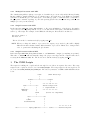
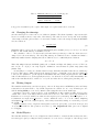
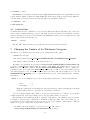
The scripts for building the coupled and the uncoupled ice models are in separate directories. The setup
scripts for the coupled model are located in ccsm3/scripts. The setup scripts for the uncoupled model
are located in ccsm3/models/ice/csim4/src. The directory structure of CSIM5 within CCSM is shown
below.
ccsm3
(main directory)
|
|
models--------+--------- scripts
|
|
|
* * * * *|* * * * *
bld------+------ice
*build scripts for*
|
|
* coupled model *
(Makefile
|
* * * * * * * * * *
macros)
|
csim4
(active ice component)
|
docs -------+------- src
|
|
(CSIM
|
documentation)
|
|
|
* * * * * * * **
bld ------------ input_templates ----+---- source ------*build scriptsr*
7
|
(Makefile macros
for uncoupled
ice model)
3.1
|
(resolution-dependent
input files)
|
(F90 source
code)
*for uncoupled *
*ice model
*
* * * * * * * **
Coupled Model Scripts
The CCSM3 scripts have been significantly upgraded from CCSM2 and are based on a completely different design philosophy. The new scripts will generate a set of ”resolved scripts” for a specific configuration
determined by the user. The configuration includes components, resolution, run type, and machine. The
run and setup scripts that were previously in the /scripts directory for CCSM2 are now generated automatically. See the CCSM3 User’s Guide for information on how to use the new scripts. The file that
contains the ice model namelist is now located in ccsm3/scripts/$CASE/Buildnml Prestage. The
script containing the environment variables used for building the executable file for the ice model is in
ccsm3/scripts/$CASE/Buildexe. The contents of the ice model namelist are described in section 4.
3.2
Uncoupled Run Script
The run script for the uncoupled model is called csim run and is located in /ccsm3/models/ice/csim4/src.
Its purpose is to coordinate setting the batch system options, the environment variables, executing the CSIM
setup script, setting up the stdout file, and submitting the model to run.
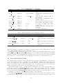
At the top of the run script, the settings for the IBM SP and the SGI Origin 2000 batch queue environments are set. These commands are machine and site dependent. Following this, the variables for the run
environment are defined. These variables are listed in Table 1.
$CASE is a character string that identifies a particular model run. It can be up to 16 characters long,
but it is best kept short, since it is used as part of the restart, history, and initial filenames. $CASESTR is a
longer string that describes a model case.
$RUNTYPE is a character string that specifies the state in which the model is to begin a run. startup and
continue are the supported run types. A startup run can be initialized by reading input from a file or from
initial conditions set within the ice model. This option is controlled by the environment variable $RESTART
in the setup script (see Section 6.1 ). Continue runs are described in Section 6.2.
$NCAT is an integer that sets the number of ice thickness categories. The default value is 5 categories. If
you are considering changing $NCAT to values other than 3 or 10, read Section 7. This is an involved process
that deserves its own section.
3.2.1
Using the Ocean Mixed Layer Model within CSIM
$OCEANMIXED ICE is a logical variable, if .true., is used to implement the slab ocean mixed layer model in
the ice model. It is a simple model that is forced using output from a POP ocean simulation. More details
on the physics of the ocean mixed layer model can be found in the Physics Documentation. It can be run
with the gx3v5 or the gx1v3 grid. To use the mixed layer model, set
setenv \$OCEANMIXED\_ICE .true.
in csim run.
3.2.2
Changing Grid Resolution
$GRID is a character string used to specify the horizontal grid. Presently, two resolutions are supported for
the ice model: gx3v5 and gx1v3. In both of these grids, the North Pole has been displaced into Greenland.
gx3v5 is the coarser grid, with longitudinal resolution of 3.6 degrees. The latitudinal resolution varies,
with a resolution of approximately 0.9 degrees near the equator. gx1v3 is the finer resolution grid, with
a longitudinal resolution of approximately one degree. Its latitudinal resolution is also variable, with a
resolution of approximately 0.3 degrees near the equator.
8
3.2.3
Changing the Number of Processors
$NX and $NY are the number of processors used by the ice model for internal parallelization. Currently, $NX
and $NY MUST divide evenly into the grid dimensions. There are checks for this in the setup script and
in the ice source code; the model will stop if these criteria are not met. $NLAT and $NLON are used for this
purpose. For load balancing purposes, $NY should be <=2. If it is greater than this, the processors assigned
subdomains near the equator will not be doing much work.
For the gx3v5 grid, the ice model is typically run on 8 tasks, with NX=4, NY=2. Running the ice model
with NX=8 and NY=1 tasks on the gx3v5 grid wil result in an error, since 8 does not divide evenly into the
100 longitude points. When this happens, the model will stop with an error message written to the log file.
If you are submitting the model to a batch queue with the number of processors modified from the
default, you will also have to modify the batch queue environment information at the top of the script. The
default setting for the IBM is:
# @ total_tasks = 8
# @ node = 1
These two lines request a total of eight MPI processes, on one 8-way node. For the NCAR SGI, the
default setting is:
# QSUB -l mpp_p=8
# request 8 processors
and for other SGI’s it may be
# BSUB -n 8
3.3
.
Uncoupled Setup Script
The purpose of the setup script, csim.setup.csh, is to build an executable version of the ice model, document
what source code and data files are being used in the ice.log.$LID file, and gather or create any necessary
input data files. $LID is a time stamp set in the run script. The environment variables set locally in the ice
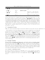
setup script are listed in Table 2.
NOTE: The variables shown in Table 2 will rarely have to be modified by the user, since they depend on
variables set in the run script. The most common changes made in the script file will be to the
namelist discussed in Section 4.
$HSTDIR, $RSTDIR and $INIDIR are the directories in $EXEROOT where the history, restart, and initial
condition files are output, respectively. The ice model input templates are located in $ICESRC. These templates are fortran modules that contain information on grid dimensions, number of ice thickness categories
and vertical resolution in the ice categories. The grid is determined in the run script and the resolution $RES is set in csim.setup.csh: 100x116 for the gx3v5 grid and 320x384 for gx1v3. Depending on
$RES and the number of ice thickness categories $NCAT set in csim run, the appropriate input template
ice model size.${RES}x${NCAT} will be copied into the directory where the ice model is being built
and renamed ice model size.F. Files exist for the following configurations:
$CSIMDIR/input
$CSIMDIR/input
$CSIMDIR/input
$CSIMDIR/input
$CSIMDIR/input
$CSIMDIR/input
$CSIMDIR/input
$CSIMDIR/input
templates/ice
templates/ice
templates/ice
templates/ice
templates/ice
templates/ice
templates/ice
templates/ice
model
model
model
model
model
model
model
model
size.F.100x116x1
size.F.100x116x3
size.F.100x116x5
size.F.100x116x10
size.F.320x384x1
size.F.320x384x3
size.F.320x384x5
size.F.320x384x10
9
Table 1: Environment Variables Set in the Run Script (csim run)
Variable
Description
CASE
case name
CASESTR
short descriptive text string, used in history files
OCEANMIXED ICE
logical variable used to implement ocean mixed layer model
ICE GRID
ice model grid (gx3v5 or gx1v3)
RUNTYPE
run type (startup or continue)
NCAT
number of thickness categories in the ice thickness distribution
NX
number of processors assigned in the x direction, used for
MPI grid decomposition
NY
number of processors assigned in the y direction, used for
MPI grid decomposition
BINTYPE
Set to MPI for internal parallelization, set to single for nonMPI runs
CSIMDIR
source code base directory
SHRCODE
share code directory
CSIMDATA
input data base directory
CBLD
makefile and Macros directory
EXEROOT
Run model, mv data, output put here
LID
timestamp for file ID string
OBJDIR
ice model code is built here
NOTE: Files exist only for certain numbers of ice thickness categories (1, 3, 5, and 10). If you need a
number of categories other than these, the model will not run as is. See Section 7 for information
on how to change the number of ice thickness categories.
The variable $OML ICE SST INIT is used if $OCEANMIXED ICE is set to .true. in the run script and
determines the initial sea surface temperature. If the run is a startup run, this variable is set to true in
the ice setup script, and the January 1 value of the sea surface temperature is read from the POP forcing
file. Thereafter, the value of $OML ICE SST INIT is set to .false., and sea surface temperature and the
freeze/melt potential is read from a restart file.
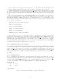
The ice model contains two namelists. The variables for both lists are set in csim.setup.csh and are
written to the file ice in in $EXEROOT when the setup script is executed. Changes to the namelists must be
made in the run or setup script, not in the ice in file. The ice model reads his file at runtime. Therefore,
Table 2: Environment Variables Set in the Ice Setup Script
Symbol
Description
HSTDIR
directory where history files are written
RSTDIR
directory where restart files are written
INIDIR
directory where initial condition files are written
ICESRC
directory where ice model input templates are located
RES
grid dimensions used to select model resolution
NLAT
number of latitudes in grid resolution
NLON
number of longitudes in grid resolution
logical variable, if true initialize ocean mixed layer temperature
OML ICE SST INIT
from within ice model
RESTART
logical variable used to initialize model from a restart file
RSTFILE
name of restart file
10
the namelist will be updated even if the ice model is not recompiled.
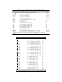
One namelist is called icefields nml and is defined in ice history.F. It contains a list of logical variables
that correspond to ice fields that will be written to the history file. By default, all these variables are set to
.true., so leaving the namelist blank will result in all fields being written to the history file. The available
fields are listed in Table 11. Changing the content of the history files via the namelist is discussed in section
8.3.3.
The other namelist is called ice nml and is defined in ice init.F. It contains variables that control the
physics used in the model. They are listed in Tables 3-8. Some of the variables in the namelist are determined
from environment variables set in the scripts. Variables that are commonly changed directly in the namelist
are the timestep dt, the length of the model run npt, and the number of subcycles per timestep in the ice
dynamics ndte.
3.4
The Build Environment
The coupled and uncoupled ice models use the same Makefile and make environment. These files are located
in the ccsm3/models/bld directory for the coupled model and in ccsm3/models/ice/csim4/src/bld
for the uncoupled model. These directories contain the following files:
• Macros.AIX contains build settings specific to AIX (IBM SP3).
• Macros.IRIX64 contains build settings specific to IRIX64 (SGI Origin).
• makdep.c evaluates the code dependencies for the source code
• Makefile is a generic gnumakefile
There is a Macros.<OS> file for each supported platform. These files contain machine dependent
preprocessor, compiler and library information for building the model. The Macros.<OS> files for the
uncoupled model have been simplified, since most of the libraries used by the coupled model are not used
by the uncoupled ice model. If you are running the model on a platform other than those tested, you will
need to create a new Macros.<OS> file and modify the paths and settings for your system. In some cases,
CSIM has a set of options that are different from the default values at the top of the file. These are after
the line ifeq ($(MODEL),csim) in the Macros.<OS> files and are described below.
3.4.1
CSIM Preprocessor Flags
Preprocessor flags are activated in the form -Doption in the Macros.<OS> files. The flags specific to the
ice model are
CPPDEFS :=
$(CPPDEFS) -Dcoupled -DNPROC_X=$(NX) -DNPROC_Y=$(NY) -D_MPI
The option -Dcoupled is set to activate the coupling interface. This will include the source code in
ice coupling.F, for example. For uncoupled runs, it has been removed. If a coupler other than the CCSM
coupler is used, there is a flag called -Dfcd coupled that will keep the fluxes from being divided by the ice
area. In coupled runs, the CCSM coupler multiplies the fluxes by the ice area, so they are divided by the
ice area in CSIM to get the correct fluxes.
The options -DNPROC X=$(NX) and -DNPROC Y=$(NY) set the number of processors used in each grid
direction. These values are set automatically in the scripts for the coupled model, and in csim run by
the user for uncoupled runs. NX and NY must divide evenly into the grid, and are used only for MPI grid
decomposition. If NX or NY do not divide evenly into the grid, the model setup will exit from the setup script
and print an error message to the ice.log* (standard out) file.
The flag -D MPI sets up the message passing interface. This must be set for runs using a parallel
environment. To get a better idea of what code is included or excluded at compile time, grep for ifdef and
ifndef in the source code or look at the *.f files in the /obj directory.
11
3.4.2
CSIM Compiler Options
The name of the Fortran compiler is set by the variable FC in the Macros.<OS> files. The default name
of the compiler is f90 on the SGI and mpxlf90 r on the IBM SP. CSIM uses the following compiler options
on the SGI platform:
FFLAGS
:= -c -64 -mips4 -O2 -r8 -i4 -show -extend_source
On the IBM, the following compiler options are set in Macros.AIX:
FFLAGS
4
:= -c -O2 -qstrict -Q -qmaxmem=-1 -qrealsize=8
-qarch=auto -qtune=auto
\
Namelist Variables
CSIM uses the same namelists for both the coupled and uncoupled models. This section describes the
namelist variables in the namelist ice nml, which determine time management, output frequency, model
physics, filenames, and options for the mixed layer ocean model. The ice namelists for the coupled model are
now located in ccsm3/scripts/$CASE/Buildnml Prestage. Modifications to the uncoupled namelist
can be made in ccsm3/models/ice/csim4/src/csim.setup.csh.
A script reads the input namelist at runtime, and writes the namelist information to the file ice in in
the directory where the model executable is located. Therefore, the namelist will be updated even if the
ice model is not recompiled. The default values of ice nml are set in ice init.F. If they are not set in the
namelist in the script, they will assume the default values listed in Tables 3-8, which list all available namelist
parameters. The default values shown here are for the coupled model, which is set up for a production run.
Several of the varialbes have different values for the uncoupeld, which is set up for a 10 day test run with
more frequent output. Only a few of these variables are required to be set in the namelist; these values are
noted in the paragraphs below. An example of the default namelist is shown in Section 4.8.1.
Varible
runid
runtype
Type
Character
Character
istep0
Integer
npt
Integer
dt
ndyn dt
ndte
Double
Integer
Integer
Table 3: Namelist Variables for Time Management
Default Value
Description
’unknown runid’
Text used in netCDF global attributes
’unknown runtype’
Determines if BASEDATE is received from
coupler or restart file
0
Step counter, number of steps taken in previous integration
99999
Total number of timesteps in a model run,
model stops when istep exceeds npt (not
used in coupled runs)
3600.
Timestep in seconds
1
Times to loop through ice dynamics
120
Number of subcycles per timestep in ice
dynamics
The time management namelist options are shown in Table 3. runid is a character string that contains
descriptive information gathered from the run script. This information is written to the global attributes in
the history files. runtype is determined from the value of $RUNTYPE set in the run script. The options for
this are discussed in section 6. istep0 is the number of steps taken in a previous integration and is written
to the restart file.
4.1
Changing the Length of the Model Run
The length of an uncoupled model run is controlled by the variable npt. It is the total number of time steps
taken in an integration. The value of npt is not used in a coupled run, since the point at which integration
12
Table 4: Maximum values for ice
Grid
min(∆x, ∆y)
gx3v5 28845.9 m
gx1v3 8558.2 m
model timestep dt
max∆t
4.0 hr
1.2 hr
is stopped is determined by the coupler. The length of a coupled run should be set in the
4.2
Changing the timestep
dt is the timestep in seconds for the ice model thermodynamics. The thermodynamics component is stable
but not necessarily accurate for any value of the timestep. The value chosen for dt depends on the stability
of the transport and the grid resolution. A conservative estimate of dt for the transport using the MPDATA
advection scheme is
∆t <
min(∆x, ∆y)
.
4max(u, v)
(1)
Maximum values for dt for the two standard CCSM POP grids, assuming max(u, v) = 0.5m/s, are shown
in Table 4. The default timestep for CSIM is one hour.
The calculation of the ice velocities is subcycled ndte times per timestep so that the elastic waves are
damped before the next timestep. The subcycling timestep is calculated as dte = dt/ndte and must be
sufficiently smaller than the damping timescale T, which needs to be sufficiently shorter than dt
dte < T < dt
(2)
This relationship is discussed in Hunke (2001); also see Hunke and Lipscomb (2002), section 4.4. The best
ratio for [dte : T : dt] is [1 : 40 : 120]. Typical combinations of dt and ndte are (3600., 120), (7200., 240)
(10800., 120).
Occasionally, ice velocities are calculated that are larger than what is assumed when the model timestep
is chosen. This causes a CFL violation in the transport scheme. A namelist option was added (ndyn dt)
to subcycle the dynamics to get through these instabilities that arise during long integrations. The default
value for this variable is one, and is typically increased to two when the ice model reaches an instability. The
value in the namelist should be returned to one by the user when the model integrates past that point.
4.3
Writing Output
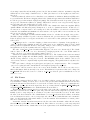
The namelist variables that control the frequency of the model diagnostics, netCDF history files, and binary
restart files are shown in Table 5. By default, diagnostics are written out once every 24 timesteps to the
ascii file ice.log.$LID (see section 8.1). $LID is a time stamp that is set in the main script.
histfreq controls the output frequency of the netCDF history files; writing monthly averages is the
default. The content of the history files is described in section 8.3. The value of hist avg determines if
instantaneous or averaged variables are written at the frequency set by histfreq. If histfreq is set to ’1’
for instantaneous output, hist avg is set to .false. within the source code to avoid conflicts. dumpfreq
and dumpfreq n control the output frequency of the binary restart files; writing one restart file per year is
the default.
If print points is .true., diagnostic data is printed out for two grid points, one near the north pole and
one near the Weddell Sea. The points are set at the top of ice diagnostics.F. This option can be helpful
for debugging.
4.4
Model Physics
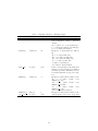
The namelist variables for the ice model physics are listed in Table 6. restart is almost always true since
most run types begin by reading in a binary restart file. See section 6 for a description of the run types and
13
Varible
diagfreq
histfreq
hist avg
dumpfreq
dumpfreq n
print points
Table 5: Namelist Variables for Writing Output
Type
Default
Description
Integer
24
Frequency of diagnostics written (min,
max, hemispheric sums) to standard
output
24 => writes once every 24 timesteps
1 => diagnostics written each timestep
0 => no diagnostics written
Character
’m’
Frequency of output written to history
file
’D’ or ’d’ writes daily data
’W’ or ’w’ writes weekly data
’M’ or ’m’ writes monthly data
’Y’ or ’y’ writes yearly data
’1’ writes every timestep
’0’ no history data is written
Logical
.true.
If true, averaged history information is
written out at a frequency determined
by histfreq. If false, instantaneous values rather than time-averages are written.
Character
’y’
Frequency restart data is written to file
’D’ or ’d’ writes restart every
dumpfreq n days
’M’ or ’m’ writes restart every
dumpfreq n months
’Y’ or ’y’ writes restart every
dumpfreq n years
’0’ no restart data is written
Integer
1
Frequency restart data is written to file
Logical
.false.
print diagnostic data for two grid points
14
Varible Name
restart
kcolumn
kitd
kdyn
kstrength
evp damping
snow into ocn
advection
grid type
albicev
albicei
albsnowv
albsnowi
no ice ic
Table 6: Namelist Variables for Model Physics
Type
Default Value
Description
Logical
.false.
If true, model is initialized using a restart
file, if false, model is initialized using initial
conditions in ice init.F.
Integer
0
Column model flag.
0 = off
1 = column model (not tested or supported)
Integer
1
Determines ITD conversion
0 = delta scheme
1 = linear remapping
Integer
1
Determines ice dynamics
0 = No ice dynamics
1 = Elastic viscous plastic dynamics
Integer
1
Determines pressure formulation
0 = Hibler (1979) parameterization
1 = Rothrock (1975) parameterization
Logical
.false.
If true, use damping procedure in evp dynamics (not supported).
Logical
.true.
If true, snow on ridged ice falls into ocean.
Character
’remap’
Determines horizontal advection scheme.
’remap’ = incremental remapping
’mpdata2’ = second order advection
’upwind’ = first order advection
Character
’displaced pole’
Determines grid type.
’displaced pole’ or ’rectangular’ (not supported)
Double
0.73
Visible ice albedo
Double
0.33
Near-infrared ice albedo
Double
0.96
Visible snow albedo
Double
0.68
Near-infrared snow albedo
Logical
.false.
Initializes ice model with no ice
15
about using restart files and internally generated model data as initial conditions. kcolumn is a flag that
will run the model as a single column if is set to 1. This option has not been thoroughly tested and is not
supported.
kitd determines the scheme used to redistribute sea ice within the ice thickness distribution (ITD) as the
ice grows and melts. The linear remapping scheme is the default and approximates the thickness distribution
in each category as a linear function (Lipscomb (2001)). The delta function method represents g(h) in each
category as a delta function (Bitz et al. (2001)). This method can leave some categories mostly empty at
any given time and cause jumps in the properties of g(h).
kdyn determines the ice dynamics used in the model. The default is the elastic-viscous-plastic (EVP)
dynamics Hunke and Dukowicz (1997). If kdyn is set to 0, the ice dynamics is inactive. In this case, ice
velocities are not computed and ice is not transported. Since the initial ice velocities are read in from the
restart file, the maximum and minimum velocities written to the log file will be non-zero in this case, but
they are not used in any calculations.
The value of kstrength determines which formulation is used to calculate the strength of the pack ice.
The Hibler (1979) calculation depends on mean ice thickness and open water fraction. The calculation of
Rothrock (1975) is based on energetics and should not be used if the ice that participates in ridging is not
well resolved.
evp damping is used to control the damping of elastic waves in the ice dynamics. It is typically set to
.true. for high-resolution simulations where the elastic waves are not sufficiently damped out in a small
timestep without a significant amount of subcycling. This procedure works by reducing the effective ice
strength that’s used by the dynamics and is not a supported option.
The value of snow into ocean determines what happens to the snow on ice that is ridged. The default
value is .true., so the snow cover on ice that undergoes ridging is put into the ocean. If this variable is
.false., the snow on ice undergoing ridging remains on the ice.
advection determines the horizontal transport scheme used. The default scheme is the incremental
remapping method (Lipscomb and Hunke (2004)). This method is less diffusive and is computationally
efficient for large numbers of categories or tracers. The MPDATA scheme is also available. It is second
order accurate, and more computationally expensive than remapping. The upwind scheme is only first order
accurate.
For coupled runs, both supported grids (gx3v5 and gx1v3) are ’displaced pole’. The ’rectangular’
option for a regular grid with constant latitude and longitude spacing is not supported.
The values of the snow and ice albedos are now set in the namelist. The ice albedos are those for ice
thicker than ahmax, which is currently set at 0.5 m. This thickness is a parameter that can be changed in
ice albedo.F. The snow albedos are for cold snow. no ice ic provides an option to initialize the ice model
with no ice cover.
4.5
File Names
The namelist parameters listed in Table 7 are for initial condition, restart, and history file and directory information. During execution, the ice model reads grid and land mask information from the files
grid file and kmt file that should be located in the executable directory. There are commands in the
scripts that copy these files from the input data directory, rename them from global $ICE GRID.grid
and global $ICE GRID.kmt to the default filenames shown in Table 7.
The namelist variable pointer file is set to the name of the pointer file containing the restart file name
that will be read when model execution begins. The pointer file resides in the scripts directory and is created
initially by the ice setup script but is overwritten every time a new restart file is created. It will contain
the name of the latest restart file. The default filename ice.restart file shown in Table 7 will not work unless
some modifications are made to the ice setup script and a file is created with this name and contains the
name of a valid restart file; this variable must be set in the namelist. More information on restart pointer
files can be found in section 8.2.
incond dir, restart dir and history dir are the directories where the initial condition file, the restart
files and the history files will be written, respectively. These values are set at the top of the setup script and
have been modified from the default values to meet the requirements of the CCSM filenaming convention.
16
Varible
grid file
kmt file
pointer file
incond dir
restart dir
history dir
incond file
dump file
history file
Table 7: Namelist Variables for File Names
Type
Default Value
Description
Character
’data.domain.grid’
Input filename containing grid information.
Character
’data.domain.kmt’
Input filename containing land mask information.
Character
’ice.restart file’
Pointer file that contains the name of
the restart file.
Character
’’
Directory where netCDF initial condition file is output.
Character
’’
Directory where restart files are output.
Character
’’
Directory where history files are output.
Character
’incond’
Root name of netCDF output initial
condition file.
Character
’iced’
Prefix for output file containing restart
information.
Character
’iceh’
Root name of history files.
Table 8: Namelist Variables for Ocean Mixed Layer Model
Type
Default Value
Description
Logical
.false.
If true, run model with ocean mixed
layer model.
oceanmixed ice file
Character
’oceanmixed ice.nc’
Name of file with ocean mixed layer
data.
oceanmixed ice sst init
Logical
.false.
If true, Jan 1 sst is read from forcing
file.
prntdiag oceanmixed
Logical
.false.
If true, print ocean mixed layer diagnostics.
Varible Name
oceanmixed ice
This allows each type of output file to be written to a separate directory. If the default values are used, all
of the output files will be written to the executable directory.
incond file, dump file and history file are the root filenames for the initial condition file, the restart
files and the history files, respectively. These strings have been determined by the requirements of the CCSM
filenaming convention, so the default values listed in Table 7 are not the same as those shown in the namelist
in Section 4.8.1. See sections 8.2 and 8.3 for an explanation of how the rest of the filename is created.
4.6
Ocean Mixed Layer Model
An ocean mixed layer model has been incorporated into the ice model since the CCSM data ocean component
does not allow frazil ice growth to occur. This is due to the minimum ocean mixed layer temperature being
fixed at the freezing point. It is a simple slab ocean mixed layer model that is forced using output from
a POP ocean simulation. More details on the physics of the ocean mixed layer model can be found in the
Physics Documentation. This option can be run with the gx3v5 or the gx1v3 grid.
The namelist variables for the ocean mixed layer model within the ice model are shown in Table 8. To
use the slab ocean model, $OCEANMIXED ICE must be set to .true. in the namelist. There are commands
in the scripts that will copy the grid dependent forcing file from the input data directory to the executable
directory and rename it oceanmixed ice.nc. This is generally not the best ocean forcing, but can be used
as a template for creating an ocean forcing file appropriate for the application.
The variable $OML ICE SST INIT determines the initial sea surface temperature. For an initial or startup
run, this variable should be set to true, and the January 1 value of the sea surface temperature will be read
17
Varible Name
atm data dir
fyear init
ocn data dir
ycycle
year init
Table 9: Namelist Variables for Atmospheric Forcing
Type
Default Value
Description
Path
Directory for atmospheric forcing
data
Integer
First year of atmospheric forcing data
Path
Directory for oceanic forcing data
Integer
Number of years in forcing data cycle
Integer
1
Initial year, if not using restart file
from the POP forcing file. For continuation runs, the value of $OML ICE SST INIT should be set to false,
and sea surface temperature and the freeze/melt potential will be read from a restart file. This variable will
be automatically set in the scripts depending on the run type. When the slab ocean mixed layer within the
ice model is used, the data that is received from the coupler from the ocean component (docn or POP) is
overwritten by the values calculated by the ocean mixed layer. Therefore, it is not appropriate to use the
ocean mixed layer option coupled to an active ocean model. Also, using the ice model with the slab ocean
mixed layer turned on, coupled to an active atmosphere and a data ocean model will require changes to the
coupler, since the ocean values calculated in the ice model will not be sent to the coupler and received by
the atmosphere component.
4.7
Atmospheric Forcing
CSIM5 can be run uncoupled using atmospheric data from 1997, available from http://www.ccsm.ucar.edu/models/ice-cs
These data files are on the low resolution grid and were created for testing the ice model. They will
not produce the best sea ice simulation. Module ice flux in.F can be modified to change the forcing data.
Namelist options for using the atmospheric forcing data are shown in Table 9. atm data dir is the root
directory where the forcing resides. fyear init and year init should be set to 1997 and ycycle should
be set to 1 for the forcing provided. ocn data dir should not be set since no ocean forcing is provided.
Subroutines in ice flux in.F are available for reading in ocean sea surface temperature and salinity data and
may be used for initializing and/or restoring the mixed layer properties; these subroutines currently are
commented out in ice flux in.F. A sample namelist using these options is shown in section 4.8.4. A brief
discussion of the atmospheric forcing files is given in section 5.1 as well as changes that should be made to
ice.F to use this forcing.
4.8
Example Namelists
This section shows several examples of namelists from the coupled and uncoupled ice models. These examples
are taken directly from csim.buildnml prestage.csh for the coupled model and from csim.setup.csh for
the uncoupled model. Most of the variables in the namelist are determined from environment variables set
elsewhere in the scripts. Since the namelists from the coupled model are ”resolved” by the scripts, meaning
that the values of most of the shell script variables are put directly into the namelist, examples are shown
for the most commonly used configurations. Variables that are commonly changed directly in the namelist
are the timestep dt and the number of subcycles per timestep in the ice dynamics ndte.
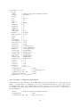
4.8.1
Example 1: CCSM Fully Coupled
The following example is the namelist used for CCSM fully coupled, or the B configuration. The variables
that are still set to shell script variables have been set at the top of csim.buildnml prestage.csh or in
other scripts. A completely resolved version of the namelist will be written to ice in in the executable
directory.
18
cat << EOF >! ice_in
&ice_nml
runid
= ’TER.01a.T85_gx1v3.B.bluesky.105608’
, runtype
= ’$runtype’
, istep0
= 0
, dt
= 3600.0
, ndte
= 120
, ndyn_dt
= 1
, npt
= 99999
, diagfreq
= 24
, histfreq
= ’m’
, dumpfreq
= ’y’
, dumpfreq_n
= 1
, hist_avg
= .true.
, restart
= $restart
, print_points = .false.
, kitd
= 1
, kdyn
= 1
, kstrength
= 1
, evp_damping
= .false.
, snow_into_ocn = .true.
, advection
= ’remap’
, grid_type
= ’displaced_pole’
, grid_file
= ’data.domain.grid’
, kmt_file
= ’data.domain.kmt’
, incond_dir
= ’$runinidir/’
, incond_file
= ’$CASE.csim.i.’
, restart_dir
= ’$runrstdir/’
, dump_file
= ’$CASE.csim.r.’
, history_dir
= ’$runhstdir/’
, history_file = ’$CASE.csim.h’
, albicev
= 0.73
, albicei
= 0.33
, albsnowv
= 0.96
, albsnowi
= 0.68
, no_ice_ic
= $no_ice_ic
, oceanmixed_ice
= .false.
, oceanmixed_ice_file
= ’oceanmixed_ice.nc’
, oceanmixed_ice_sst_init
= .false.
, prntdiag_oceanmixed
= .false.
, pointer_file = ’rpointer.ice’
/
4.8.2
Example 2: Coupled Ice Only Model
This example is the M configuration. It is CSIM with the latm data atmosphere model, data land model,
and the ocean mixed layer model within the ice model all communicating through the coupler. The following
modifications will be made to the namelist when the resolved scrips are created for the M configuration. See
the CCSM3 User’s Guide (http://www.ccsm.ucar.edu/models/ccsm3.0/ccsm) on how to create scripts for
the M configuration.
runid
= ’TER.01a.T62_gx1v3.M.bluesky.095234’
, oceanmixed_ice
= .true.
, oceanmixed_ice_sst_init
= $oml_ice_sst_init
19
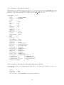
4.8.3
Example 3: Uncoupled Ice Model
This example is the namelist from the uncoupled ice model that resides in the file csim.setup.csh. npt
has been modified, since it determines the length of the uncoupled run. The snow and ice albedos used by
CCSM are not set in the name list. The default values set in ice init.F are used.
cat << EOF >! ice_in
&ice_nml
runid
= ’$CASE $CASESTR’
, runtype
= ’$RUNTYPE’
, istep0
= 0
, dt
= 3600.0
, ndyn_dt
= 1
, ndte
= 120
, npt
= 240
, diagfreq
= 24
, histfreq
= ’m’
, dumpfreq
= ’d’
, dumpfreq_n
= 5
, hist_avg
= .true.
, restart
= $RESTART
, print_points = .false.
, kitd
= 1
, kdyn
= 1
, kstrength
= 1
, evp_damping = .false.
, snow_into_ocn = .true.
, advection
= ’remap’
, grid_type
= ’displaced_pole’
, grid_file
= ’data.domain.grid’
, kmt_file
= ’data.domain.kmt’
, incond_dir
= ’$INIDIR/’
, incond_file = ’$CASE.csim.i.’
, restart_dir = ’$RSTDIR/’
, dump_file
= ’$CASE.csim.r.’
, history_dir = ’$HSTDIR/’
, history_file = ’$CASE.csim.h’
, pointer_file = ’$CSIMDIR/rpointer.ice’
, oceanmixed_ice
= $OCEANMIXED_ICE
, oceanmixed_ice_file
= ’oceanmixed_ice.nc’
, oceanmixed_ice_sst_init
= $OML_ICE_SST_INIT
, prntdiag_oceanmixed
= .false.
/
4.8.4
Example 4: Uncoupled Ice Model with Atmospheric Forcing
To run the uncoupled ice model with atmospheric forcing, the following options should be added to the
above namelist:
,
,
,
,
ycycle
year_init
fyear_init
atm_data_dir
=
=
=
=
1
1997
1997
’/ptmp/$LOGNAME/csim_forcing/atm/gx3v5/’
20
4.8.5
Example 5: History File Namelist
The second namelist controls what variables are written to the history file. By default, all files are written to
the history file. Variables that are not output are set in the namelist icefields nml. Some of the following
fields are not written to the history file since they can be retrieved from the ocean history files. The melt
and freeze onset fields are not used, since the information they contain may not be correct if the model is
restarted mid-year. The ice areas and volumes for categories six through ten are not used, since the default
thickness distribution consists of five ice categories.
&icefields_nml
f_sst
=
, f_sss
=
, f_uocn
=
, f_vocn
=
, f_frzmlt
=
, f_strtltx
=
, f_strtlty
=
, f_mlt_onset =
, f_frz_onset =
, f_aice6
=
, f_aice7
=
, f_aice8
=
, f_aice9
=
, f_aice10
=
, f_vice1
=
, f_vice2
=
, f_vice3
=
, f_vice4
=
, f_vice5
=
, f_vice6
=
, f_vice7
=
, f_vice8
=
, f_vice9
=
, f_vice10
=
/
5
.false.
.false.
.false.
.false.
.false.
.false.
.false.
.false.
.false.
.false.
.false.
.false.
.false.
.false.
.false.
.false.
.false.
.false.
.false.
.false.
.false.
.false.
.false.
.false.
Model Input Datasets
Both the coupled and uncoupled CSIM require a minimum of three files to run:
• global ${ICE GRID}.grid is a binary file containing grid information and is renamed
data.domain.grid
when it is copied to the executable directory.
• global ${ICE GRID}.kmt is a binary file containing land mask information and is renamed
data.domain.kmt.
• iced.0001-01-01.${ICE GRID}.20lay or iced.0001-01-01.gx3v5.040213 are binary files containing initial condition information for the gx1v3 and gx3v5 grids, respectively. The thickness distribution
in this restart file contains 5 categories, each with 4 layers.
Depending on the grid selected in the scripts, the appropriate global* and iced* files will be copied and
renamed in the executable directory. Currently, only gx3v5 and gx1v3 grids are supported for the ice and
ocean models.
21
An additional data file is necessary to use the ocean mixed layer within the ice model, depending on the
specified grid:
• pop frc gx1v3 010815.nc contains monthly averaged ocean forcing from POP output.
• pop frc gx3v5 040212.nc same as above, but for the gx3v5 grid.
This file is renamed oceanmixed ice.nc when it is copied into the executable directory.
5.1
Atmospheric Forcing
The uncoupled ice model will run without atmospheric forcing. It will use the fluxes set in subroutine
init flux. For atmospheric forcing, the following datasets are available on the gx3v5 grid, and can be read in
using the module ice flux in.F. The directory where the data is located will have to be set in this module,
and not in the scripts. The files are as follows:
/wherever/you/put/it/atm/gx3v5/ISCCPM/MONTHLY/RADFLX/cldf.1997.dat
/wherever/you/put/it/atm/gx3v5/ISCCPM/MONTHLY/RADFLX/swdn.1997.dat
/wherever/you/put/it/atm/gx3v5/MXA/MONTHLY/PRECIP/prec.1997.dat
/wherever/you/put/it/atm/gx3v5/NCEP/4XDAILY/STATES/dn10.1997.dat
/wherever/you/put/it/atm/gx3v5/NCEP/4XDAILY/STATES/q 10.1997.dat
/wherever/you/put/it/atm/gx3v5/NCEP/4XDAILY/STATES/t 10.1997.dat
/wherever/you/put/it/atm/gx3v5/NCEP/4XDAILY/STATES/u 10.1997.dat
/wherever/you/put/it/atm/gx3v5/NCEP/4XDAILY/STATES/v 10.1997.dat
These files are in direct access binary files, and the source is evident from the path names. cldf.1997.dat
and swdn.1997.dat contain the monthly averaged cloud fraction and downwelling shortwave. prec.1997.dat
is the monthly averaged precipitation in mm/month. The remaining files are the atmospheric density, specific humidity, air temperature, and wind fields. Note that these datasets are meant for testing the model
and are not the best observational data for research. Users are advised not to publish results based on these
datasets. To use this forcing, the following lines in ice.F need to be uncommented:
call init_getflux
call getflux
6
Run Types
The run types available for the coupled model are described in the CCSM User’s Guide. There are two run
types available for the uncoupled ice model and are described in this section.
6.1
Startup Runs
If $RUNTYPE is set to startup, the model will read in the restart file that resides in $CSIMDATA called
iced.0001-01-01.$ICE GRID.20lay. The conditions in this file are for the gx1v3 grid and are from an
equilibrium run using modified NCEP forcing. The setup script will create a pointer file named rpointer.ice
with the name of the initial restart file in it Startup runs can also be initialized using data created within
the ice model, as described in the next section.
Using Initial Conditions from within CSIM
Initial conditions can be calculated within the ice model in a subroutine called init state in ice init.F. Here,
the ocean surface is initialized at the freezing point everywhere north of 40 degrees and south of -40 degrees
latitude, allowing ice to form everywhere in these regions. While running the ice model with a data ocean
will melt any extra ice during the first year of integration, is not recommended that these initial conditions
be used when running the ice model coupled to an active ocean model. The advantage of using this input is
that it is not grid or land mask dependent. To use these initial conditions, set $RESTART in csim.setup.csh:
22
set RESTART = .false.
Initializing the model using a restart file from an equilibrium run will result in a more physically reasonable
scenario than the initial conditions set within CSIM. The drawbacks are that the data is binary, difficult to
edit, and is date and grid dependent. A restart file will be used as initial conditions if
set RESTART = .true.
in csim.setup.csh.
6.2
Continue Runs
A continue run is an exact continuation of a previous run. This means that the run will produce a bit-for-bit
answer as if the existing run had not stopped. The input data file is determined by the filename set in the
restart pointer file (see section 8.2). It is assumed that $CASE has not changed. For a continue run, the only
change required in the run script is to set:
RUNTYPE
continue
The date will continue from the previous run, since it is read in from the restart file.
7
Changing the Number of Ice Thickness Categories
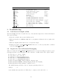
The number of ice thickness categories affects ice model input files in three places:
• $NCAT in the run script
• The input template files ice model size.F.$RESx$NCAT in $CSIMDIR/input templates
• The initial condition (restart) file in the input file directory
The number of ice thickness categories is set in ccsm3/scripts/$CASE/Buildexe/csim.buildexe.csh
(coupled) or csim run (uncoupled) using the variable called $NCAT. The default value is 5 categories.
$NCAT is used to determine which module ice model size.F.$RESx$NCAT is copied to /obj before
compilation where it is renamed ice model size.F. $RES is the resolution of the grid, 100x116 (gx3v5)
and 320x384 (gx1v3) for low and high resolution grids, respectively. The input templates are located in
$CSIMDIR/input templates for 1, 3, 5 and 10 thickness categories on the default grid sizes of 100x116
and 320x384.
NOTE: To use one ice thickness category, the following changes will need to be made in the namelist:
, kitd
, kstrength
= 0
= 0
With these settings, the model will use the delta scheme instead of linear remapping and a strength
parameterization based on open water area and mean ice thickness.
To create an input template with a number of categories other than the above values, copy an existing
template that has the desired grid. Change ncat to the appropriate number of categories.
The information in the initial restart file is dependent on the number of ice thickness categories and the
total number of layers in the ice distribution. An initial condition file exists only for the default case of 5
ice thickness categories, with four layers in each category. To create an initial condition file for a different
number of categories or layers, these steps should be followed:
• Set $NCAT to the desired number of categories in csim run (uncoupled) or
ccsm3/scripts/$CASE/Buildexe/csim.buildexe.csh (coupled).
23
• Set the namelist variable dumpfreq = ’m’ in csim.setup.csh (uncoupled) or
ccsm3/scripts/$CASE/Buildnml Prestage/csim.buildnml prestage.csh
(coupled) to print out restart files monthly.
• Set the namelist variable restart = .false. in csim.setup.csh (uncoupled) or
ccsm3/scripts/$CASE/Buildnml Prestage/csim.buildnml prestage.csh
(coupled) to use the initial conditions within the ice model.
• Create an input template (or use an existing one) with the desired number of categories.
• Run the model to equilibrium.
• The last restart file can be used as an initial condition file.
• Change the name of the last restart file to iced.0001-01-01.$GRID.
• Copy the file into the input data directory or directly into the /rest directory under the executable
directory.
Note that the date printed inside the binary restart file will not be the same as 0001-01-01. For coupled
runs, $BASEDATE will be the starting date and the date inside the file will not be used. For uncoupled runs,
the starting date may have to be set in the code or changed in the restart file.
8
Output Data
The ice model produces three types of output data. A file containing ASCII text, also known as a log file, is
created for each run that contains information about how the run was set up and how it progressed. A series
of binary restart files necessary to continue the run are created. A series of netCDF history files containing
gridded instantaneous or time-averaged output are also generated during a run. These are described below.
8.1
Stdout Output
Diagnostics from the ice model are written to an ASCII file that contains information from the compilation,
a record of the input parameters, and how hemispherically averaged, maximum and minimum values are
evolving with the integration. Certain error conditions detected within the ice setup script or the ice model
will also appear in this file. Upon the completion of the simulation, some timing information will appear at
the bottom of the file. The file name is of the form ice.log.$LID, where $LID is a timestamp for the file
ID. It resides in the executable directory. The frequency of the diagnostics is determined by the namelist
parameter diagfreq.
8.2
Restart Files
Restart files contain all of the initial condition information necessary to restart from a previous simulation.
These files are in a standard IEEE 64 bit binary format. A restart file is not necessary for an initial run,
but is highly recommended. The initial conditions that are internal to the ice model produce an unrealistic
ice cover that an uncoupled ice model will correct in several years. The initial conditions from a restart file
are created from an equilibrium solution, and provide more realistic information that is necessary if coupling
to an active ocean model. The frequency at which restart files are created is controlled by the namelist
parameter dumpfreq. The names of these files are proceeded by the namelist parameter dump file and, by
default are written out yearly to the /rest directory under the executable directory. To change the directory
where these files are located, modify the variable $RSTDIR at the top of the setup script. The names of the
restart files follow the CCSM Output Filename Requirements. The form of the restart file names are as
follows:
$CASE.csim.r.yyyy-mm-dd-sssss
24
For example, the file $CASE.csim.r.0002-01-01-00000 would be written out at the end of year 1,
month 12. A file containing the name of a restart file is called a restart pointer file. This filename information
allows the model simulation to continue from the correct point in time, and hence the correct restart file.
Restart Pointer Files
A pointer file is an ascii file named rpointer.ice that contains the path and filename of the latest restart
file. The model uses this information to find a restart file from which initialization data is read. The pointer
files are written to and then read from the executable directory. For startup runs, a pointer is created by
the ice setup script Whenever a restart file is written, the existing restart pointer file is overwritten. The
namelist variable pointer file contains the name of the pointer file. Pointer files seldom need editing. The
contents are usually maintained by the setup script and the component model.
8.3
History Files
History files contain gridded data values written at specified times during a model run. By default, the
history files will be written to the directory history dir defined in the namelist. The netCDF file names
are prepended by the character string given by history file in the ice nml namelist. This character string
has been set according to CCSM Output Filename Requirements. If history file is not set in the namelist,
the default character string ’iceh’ is used. The user can specify the frequency at which the data are written.
Options are also available to record averaged or instantaneous data. The form of the history file names are
as follows:
Yearly averaged: $CASE.csim.h.yyyy.nc
Monthly averaged: $CASE.csim.h.yyyy-mm.nc
Weekly averaged: $CASE.csim.hw.yyyy-mm-dd-sssss.nc
Daily averaged: $CASE.csim.h.yyyy-mm-dd.nc
Instantaneous (histfreq = ’y’, ’m’, ’w’ or ’d’): $CASE.csim.h.yyyy-mm-dd-sssss.nc
Instantaneous (written every dt, histfreq = 1): $CASE.csim.h.yyyy-mm-dd-sssss.nc
$CASE is set in the main setup script. All history files are written to /hist in the executable directory.
Changes to the frequency and averaging will affect all output fields. The best description of the history
data comes from the file itself using the netCDF command ncdump -h filename.nc. Variables containing
grid information are written to every file and are listed in Table 10. In addition to the history files, a
netCDF file containing a snapshot of the initial ice state is created at the start of each run. The file name
is $CASE.csim.i.yyyy-mm-dd-sssss.nc and is written to /init in the executable directory.
8.3.1
Caveats Regarding Averaged Fields
In computing the monthly averages for output to the history files, most arrays are zeroed out before being
filled with data. These zeros are included in the monthly averages where there is no ice. For some fileds,
this is not a problem, for example, ice thickness and ice area. For other fields, this will result in values that
are not representative of the field when ice is present. Some of the fields affected are:
• Flat, Fsens - latent and sensible heat fluxes
• albsni - snow/ice broadband albedo
• evap - evaporative water flux
• Fhnet - ice/ocn net heat flux
• Fswabs - snow/ice/ocn absorbed solar flux
• strairx, strairy - zonal and meridional atm/ice stress
• strcorx, strcory - zonal and meridional coriolis stress
25
For some fields, a non-zero value is set where there is no ice. For example, Tsfc has the freezing point
averaged in, and Flwout has σTf4 averaged in. At lower latitudes, these values can be erroneous.
To aid in the interpretation of the fields, a field called ice present is written to the history file. It contains
information on the fraction of the time-averaging interval when any ice was present in the grid cell during
the time-averaging interval in the history file. This will give an idea of how many zeros were included in the
average.
The second caveat results from the coupler multiplying fluxes it receives from the ice model by the ice
area. Before sending fluxes to the coupler, they are divided by the ice area in the ice model. These are the
fluxes that are written to the history files, they are not what affects the ice, ocean or atmosphere, nor are
they useful for calculating budgets. The division by the ice area also creates large values of the fluxes at the
ice edge. The affected fields are:
• Flat, Fsens - latent and sensible heat fluxes
• Flwout - outgoing longwave
• evap - evaporative water flux
• Fresh - ice/ocn fresh water flux
• Fhnet - ice/ocn net heat flux
• Fswabs - snow/ice/ocn absorbed solar flux
When applicable, two of the above fields will be written to the history file: the value of the field that
is sent to the coupler (divided by ice area) and a value of the flux that has been multiplied by ice area
(what affects the ice). Fluxes multiplied by ice area will have the suffix aice appended to the variable
names in the history files. Fluxes sent to the coupler will have ”sent to coupler” appended to the long name.
Fields of rainfall and snowfall multiplied by ice area are written to the history file, since the values are valid
everywhere and represent the precipitation rate on the ice cover.
8.3.2
Changing Frequency and Averaging
The frequency at which data are written to a history file as well as the interval over which the time average is
to be performed is controlled by the namelist variable histfreq. Data averaging is invoked by the namelist
variable hist avg. The averages are constructed by accumulating the running sums of all variables in
memory at each timestep. The options for both of these variables are described in Table 5. If hist avg is
true, and histfreq is set to monthly, for example, monthly averaged data is written out on the last day of
the month.
8.3.3
Changing Content
The second namelist in the setup script controls what variables are written to the history file. To remove
a field from this list, add the name of the logical variable associated with that field to the &icefields nml
namelist in csim.buildnml prestage.csh (coupled) or csim.setup.csh (uncoupled) and assign it a value
of .false.. For example, to remove ice thickness and snow cover from the history file, add
&icefields_nml
f_hi
= .false.
, f_hs
= .false.
/
to the namelist.
Table 11: Standard Fields Available for Output to History File
26
Table 10: Time and Grid Information Written to History File
Field
Description
time
model time
time bounds boundaries for time-averaging interval
TLON
T grid center longitude
TLAT
T grid center latitude
ULON
U grid center longitude
ULAT
U grid center latitude
tmask
ocean grid mask (0=land, 1=ocean)
tarea
T grid cell area
uarea
U grid cell area
dxt
T cell width through middle
dyt
T cell height through middle
dxu
U cell width through middle
dyu
U cell height through middle
HTN
T cell width North side
HTE
T cell width East side
ANGLET
angle grid makes with latitude line on T grid
ANGLE
angle grid makes with latitude line on U grid
ice present fraction of time-averaging interval that any ice is present
Logical Variable
f hi
f hs
f Tsfc
f aice
f aice1
f aice2
f aice3
f aice4
f aice5
f aice6
f aice7
f aice8
f aice9
f aice10
f vice1
f vice2
f vice3
f vice4
f vice5
f vice6
f vice7
f vice8
f vice9
f vice10
f uvel
Description
grid box mean ice thickness
grid box mean snow thickness
snow/ice surface temperature
ice concentration (aggregate)
ice concentration (category 1)
ice concentration (category 2)
ice concentration (category 3)
ice concentration (category 4)
ice concentration (category 5)
ice concentration (category 6)
ice concentration (category 7)
ice concentration (category 8)
ice concentration (category 9)
ice concentration (category 10)
ice volume (category 1)
ice volume (category 2)
ice volume (category 3)
ice volume (category 4)
ice volume (category 5)
ice volume (category 6)
ice volume (category 7)
ice volume (category 8)
ice volume (category 9)
ice volume (category 10)
zonal ice velocity
continued on next page
27
Units
m
m
C
%
%
%
%
%
%
%
%
%
%
%
m
m
m
m
m
m
m
m
m
m
cm s−1
Units
days
days
degrees
degrees
degrees
degrees
m2
m2
m
m
m
m
m
m
radians
radians
continued from previous page
f
f
f
f
f
f
f
f
f
f
f
f
f
f
f
f
f
f
f
f
f
f
f
f
f
f
f
f
f
f
f
f
f
f
f
f
f
f
f
f
f
f
f
f
f
f
f
f
vvel
fswdn
flwdn
snow
snow ai
rain
rain ai
sst
sss
uocn
vocn
frzmlt
fswabs
fswabs ai
albsni
aldvr
aldvi
flat
flat ai
fsens
fsens ai
flwout
flwout ai
evap
evap ai
Tref
Qref
congel
frazil
snoice
meltb
meltt
meltl
fresh
fresh ai
fsalt
fsalt ai
fhnet
fhnet ai
fswthru
fswthru ai
strairx
strairy
strtltx
strtlty
strcorx
strcory
strocnx
meridional ice velocity
downwelling solar flux
downwelling longwave flux
snow fall rate received from coupler
snow fall rate on ice cover
rain fall rate received from coupler
rain fall rate on ice cover
sea surface temperature
sea surface salinity
zonal ocean current
meridional ocean current
freeze/melt potential
absorbed solar flux sent to coupler
absorbed solar flux in snow/ocn/ice
snow/ice broad band albedo
visible direct albedo
near-infrared direct albedo
latent heat flux sent to coupler
ice/atm latent heat flux
sensible heat flux sent to coupler
ice/atm sensible heat flux
outgoing longwave flux sent to coupler
ice/atm outgoing longwave flux
evaporative water flux sent to coupler
ice/atm evaporative water flux
2 m reference temperature
2 m reference specific humidity
basal ice growth
frazil ice growth
snow-ice formation
basal ice melt
surface ice melt
lateral ice melt
ice/ocn fresh water flux sent to coupler
ice/ocn fresh water flux
ice to ocn salt flux sent to coupler
ice to ocn salt flux
ice/ocn net heat flux sent to coupler
ice/ocn net heat flux
SW transmitted through ice to ocean sent to coupler
SW transmitted through ice to ocean
zonal atm/ice stress
meridional atm/ice stress
zonal sea surface tilt
meridional sea surface tilt
zonal coriolis stress
meridional coriolis stress
zonal ocean/ice stress
continued on next page
28
cm s−1
W m−2
W m−2
cm day−1
cm day−1
cm day−1
cm day−1
C
g kg−1
cm s−1
cm s−1
W m−2
W m−2
W m−2
%
%
%
W m−2
W m−2
W m−2
W m−2
W m−2
W m−2
cm day−1
cm day−1
C
g/kg
cm day−1
cm day−1
cm day−1
cm day−1
cm day−1
cm day−1
cm day−1
cm day−1
kg m−2 day−1
kg m−2 day−1
W m−2
W m−2
W m−2
W m−2
N m−2
N m−2
m m−1
m m−1
N m−2
N m−2
N m−2
continued from previous page
f
f
f
f
f
f
f
f
f
f
f
f
f
f
f
9
strocny
strintx
strinty
strength
divu
shear
opening
sig1
sig2
daidtt
daidtd
dvidtt
dvidtd
mlt onset
frz onset
meridional ocean/ice stress
zonal internal ice stress
meridional internal ice stress
compressive ice strength
velocity divergence
strain rate
lead opening rate
normalized principal stress component
normalized principal stress component
area tendency due to thermodynamics
area tendency due to dynamics
ice volume tendency due to thermo.
ice volume tendency due to dynamics
melt onset date
freeze onset date
N m−2
N m−2
N m−2
N m−1
% day−1
% day−1
% day−1
% day−1
% day−1
cm day−1
cm day−1
Troubleshooting
9.1
Code does not Compile or Run
Check the ice.log.* file in the executable directory, or the standard output and error files for information.
Also, try the following:
• Delete the executable directory and rebuild the model.
• Make sure that there is a Macros.<OS> file for your platform. Modify the directory paths for the
libraries.
• Make sure all paths and file names are set correctly in the scripts.
• If changes were made to the ice model size.F file in the source code directory, they will be overwritten
by the file in input templates.
9.2
Negative Ice Area in Horizontal Remapping
This error is written from ice transport remap.F when the ice model is checking for negative ice areas.
If it happens well into a model integration, it can be indicative of a CFL violation. The output looks like:
60: New area < 0, istep = 119588
60: (my_task,i,j,n) = 4 21 380 1
60: Old area = 0.960675000975677174E-05
60: New area = -0.161808948357841311E-06
60: Net flux = -0.976855895811461324E-05
60:(shr_sys_abort) ERROR: remap transport: negative area
60:(shr_sys_abort) WARNING: calling shr_mpi_abort() and stopping
60:(shr_mpi_abort):remap transport: negative area 0
The dynamics timestep should be reduced to integrate past this problem. Set
, ndyn_dt
= 2
in the namelist and restart the model. When the job completes set the value back to 1.
29
9.3
Conservation Error
This error is written from ice itd.F when the ice model is checking that initial and final values of a conserved
field are equal to within a small value. The output looks like:
Conservation error: vice, add_new_ice
11 : 14 185
Initial value = 1362442.600400560
Final value = 1362442.600400561
Difference = 2.328306436538696D-10
(shr_sys_abort) ERROR: ice: Conservation error
(shr_sys_abort) WARNING: calling shr_mpi_abort() and stopping
(shr_mpi_abort):ice: Conservation error 0
Non-conservation can ocur if the ice model is receiving very bad forcing, and is not able to deal with it.
This has occurred after a CFL violation in the ocean. The timestep in the ocean may be decreased to get
around the problem.
9.4
MPDATA transport unstable
The ice model dynamics is subcycled ndte times per timestep so that the elastic waves are damped before
the next timestep. When the value of ndte is too small, an instability occurs, the model execution stops,
and an error message similar to this example is written out to the log file:
mpdata phi = -0.122707896960329384E-05 n = 5
(shr_sys_abort) ERROR: (mpdata) transport unstable
(shr_sys_abort) WARNING: calling mpi_abort() and stopping
To get around this problem, increase the value of ndte in the namelist. Reasonable values of this
parameter are discussed in section 4.2. The model run can be restarted from the last set of restart files that
were written before the execution halted.
9.5
NX does not divide evenly into grid
If you modify the number of tasks used by the ice model, the model may stop with this error written to the
log file:
’ERROR: NX must divide evenly into grid,100,8’
The number of MPI processors used by the ice model must divide evenly into the grid dimensions. For
example, running the ice model with 8 tasks on the gx3v5 grid will result in an error, since 8 does not divide
evenly into the 100 longitude points. To fix this error, change the value of $NTASKS for the uncoupled ice
model in the main script. In this case, a value of 4 would work, and the task geometry would also have to
be changed.
9.6
Enabling the Debugger
This section explains how to set some compiler options for debugging. For the coupled model, set DEBUG
to TRUE in the env run script. For the uncoupled ice model, set setenv DEBUG TRUE in csim.setup.csh.
Before running the model, be sure to delete the object files so that the source code will be recompiled. If a
core file is created, it will be in the executable directory. Use dbx to look at the core file. Useful information
may also appear in the standard error and output files.
30
9.7
Unit 50 Error
Unit 50 is the restart file. If the path or file name in the rpointer.ice file is incorrect, or the restart file
does not exist in the /rest directory below the executable directory, the model will stop with this message:
8:1525-014 The I/O operation on unit 50 cannot be completed because an errno value
of 2 (A file or directory in the path name does not exist.) was received
while opening the file. The program will stop.
Verify that the path and file name in the rpointer are correct and that the restart file exists in the correct
location.
31
References
Bitz, C. M., M. Holland, M. Eby and A. J. Weaver, 2001: Simulating the ice-thickness distribution in a
coupled climate model. J. Geophys. Res., 106, 2441–2463.
Bitz, C. M. and W. H. Lipscomb, 1999: An energy-conserving thermodynamic model of sea ice. J. Geophys.
Res., 104, 15,669–15,677.
Hibler, W. D., 1979: A dynamic thermodynamic sea ice model. J. Phys. Oceanogr., 9, 815–846.
Hunke, E. C., 2001: Viscous-plastic sea ice dynamics with the evp model: Linearization issues. J. Comp.
Phys., 170, 18–38.
Hunke, E. C. and J. K. Dukowicz, 1997: An elastic-viscous-plastic model for sea ice dynamics. J. Phys.
Oceanogr., 27, 1849–1867.
Hunke, E. C. and J. K. Dukowicz, 2003: The sea ice momentum equation in the free drift regime. Los Alamos
National Laboratory,Tech. Rep. LA-UR-03-2219.
Hunke, E. C. and W. H. Lipscomb, 2002: CICE: the Los Alamos sea ice model, documentation and software
User’s Manual. T-3 Fluid Dynamics Group, Los Alamos National Laboratory, Tech. Rep. LACC-98-16
v.3.
Hunke, E. C. and W. H. Lipscomb, 2004: CICE: the Los Alamos Sea Ice Model, Documentation and Software
User’s Manual. T-3 Fluid Dynamics Group, Los Alamos National Laboratory, Tech. Rep. LA-CC-98-16
v.3.1.
Lipscomb, W. H., 2001: Remapping the thickness distribution in sea ice models. J. Geophys. Res., 106,
13,989–14,000.
Lipscomb, W. H. and E. C. Hunke, 2004: Modeling sea ice transport using incremental remapping. Mon.
Wea. Rev., in press.
Rothrock, D. A., 1975: The energetics of the plastic deformation of pack ice by ridging. J. Geophys. Res.,
80, 4514–4519.
Thorndike, A. S., D. S. Rothrock, G. A. Maykut and R. Colony, 1975: The thickness distribution of sea ice.
J. Geophys. Res., 80, 4501–4513.
32