1
Advanced Modelling
of
Sports Footwear
by
Paul J. Gibbs
A Doctoral Thesis
Submitted in Partial Fulfilment of the Requirements
for award of
Doctor of Philosophy
of
Loughborough University
Chapter 4
Literature Review:
Finite Element Analysis
4.1
Introduction
This chapter presents a very brief overview of the finite element method of structural analysis
- a subject which can fill many libraries. A short introduction is followed by reviews of the
most advanced (and applicable) models in the public domain at the time of writing. It is
expected that models of shoes are being created and used by major manufacturers, but the
competitive nature of the footwear industry means these models are unlikely to be released
into the public domain in the near future (if at all). Modelling of the human foot has been
included as most of the work on shoes to date has come out of a need for analysis of medical
footwear, almost all of which developed as an extension of a foot model. The final section
goes into more detail regarding the use of ABAQUS, the finite element software used in this
research.
This chapter does not aim to assess the required accuracy of the various models that will
come out of this research, this is to be achieved through physical testing of footwear samples
and parts, and is discussed in Chapters 7-9.
4.2
The Finite Element Method
Finite element analysis is a theoretical mathematical method of predicting the solution to a
physical problem by dividing (discritising) the geometry of the problem into small sections
(elements). It is normally used when the precise, analytical solution is too complex to be
solved (in the time available), and practical testing is either inefficient or not possible. Each
element is analysed using relatively simple mathematics and will normally have a linear
or quadratic variation of the desired property with length. The large number of simple
calculations required for a FEA solution are suited to processing by computer, and the vast
majority of FE analyses are now done in this way (except for teaching purposes, where the
problems used are very simple). A major advantage of FE over practical testing is that once
a model has been verified (proven to be satisfactorily accurate), there is a high likelihood
that the internal stresses in the model are similar to that in the real test situation, allowing
the user to probe the inner workings of whatever is being modelled. This can be extremely
difficult to do, and sometimes impossible, with real testing.
A FE model is normally constructed from geometry, which is discritised into a mesh; a
representation of all the elements in the model, connected by nodes. Each node has a given
57
number of degrees of freedom (variables in the model). Generally these are the 6 spatial
degrees of freedom, but others are available, for example: temperature, conductivity and
inertia. External forces, fixings and contact between ‘objects’ are also assigned (known as
boundary conditions) to either/both nodes or elements. The elements are assigned mechanical
properties (e.g. stiffness) and the problem is then solved in matrix form with appropriate
manipulations to give the solution. The size of the matrices directly affects the time taken
to process the solution and this in turn is affected by the number of degrees of freedom and
complexity of the boundary conditions, as well as of course the processing capabilities of the
computer used.
Incorrect specification of any of the material parameters, geometry or boundary conditions, coupled with some unavoidable assumptions that must be made when using the FE
technique mean that inaccuracies will be present in the model. It is the job of the FE analyst
to be aware of, quantify, minimise and where possible, correct for these inaccuracies.
4.3
Material FEA
The first step in creating an accurate model of a midsole is to model the basic materials
that it is made of (in this case mostly EVA foam and TPU). If mechanical tests with simple
geometry cannot be modelled correctly then a complex full shoe model will be inaccurate,
and therefore of limited use, unless the inconsistencies can be assessed and quantified.
A material model is usually created by fitting an equation to test data, the main equation
types being linear (e.g. metals in the elastic region), hyperelastic (high strain incompressible
materials, e.g. rubber, TPU) and hyperfoam (high strain, highly compressible, e.g. EVA
foam). Details on which material models have been used in the shoe models in this thesis
are given in Chapter 7.
Material modelling with FEA can be divided into constitutive and macro-scale models,
where the former considers the atomic/molecular response of idealised materials, while the
latter works on a larger scale overall response. The equations used in constitutive modelling
are normally based on the mechanics of the molecular structure, while macro-scale models
use curve fitting techniques. Knowledge of how the models work in principle is essential to
using them correctly in a model, however this research will only use current material models’
mathematics, and not attempt to develop new equations or fits.
D’Agati (1993) performed linear and non-linear elastic FEA on a simple representation of
a midsole, using force input data collected from in-shoe measurements (vertical force only).
A single 20-node cube (quadratic) element was used to assess the stress/strain curve, and
then this data was used in the midsole model (using the same element type). No numerical
results were given, but the paper quotes:
Differences between the linear model’s peak stresses and strains varied from -98%
to 680% with respect to the non-linear model’s results.
This is attributed to the non-linear response of the EVA material used.
Swigart (1995) used a vertical impact drop test with an 8.5 kg missile impacting onto
‘midsole specimens’ (the exact nature of these specimens is not specified). Tests results were
then applied to an isotropic linear viscoelastic material model and FEA performed. Good
correlation was reported for impact heights of 13 & 25 mm, but from 50 mm upwards, the
model deviates from the practical results. As an example of this deviation the 50 mm result
is shown in Figure 4.1).
58
"!
#"$%&
"'('!
!
Figure 4.1: Drop tests results from 8.5 kg mass falling from 50 mm onto midsole foam; average
test values and model predications are shown. Reproduced from Swigart (1995).
Shiang (1997) used FE to study the cushioning response of an unspecified midsole material. Material properties were obtained from compression of a cylindrical specimen under
loading by a vertical actuator (Instron machine). Loading values were taken from in-shoe
measurements and an assumed shear force of 1/10th of the peak vertical loading was applied
to the model (shown in Figure 4.2). Both linear and hyperfoam material models were used,
along with different boundary conditions, and models that included combinations of midsole/insole/insole board. It is not clear if the results of the study were verified by comparing
real compression of the midsole with the model results.
Figure 4.2: FE mesh of a simple EVA shoe heel. Shiang (1997).
The response of the foam in car seats was studied by Pajon (1996). Mechanical tests
were performed and the test data used to verify the material models. The report notes the
importance of verifying the simple material models with complex real parts, as the car seat
foam is in a combination of compression and tension and may not be modelled accurately
with uniaxial mechanical tests (as can be seen in Figure 3.31).
Thomson (1999) used uni-axial test data to create a hyperfoam material model, and used
this to model the heel impact. To reduce processing time, only a cylindrical section of the
heel was modelled (this allowed a 2D axisymmetric model, as shown in Figure 4.3). The
model was pinned at the base and the nodes on the vertical walls were constrained to move
in the vertical direction only. The accuracy of these boundary conditions is questionable and
may require practical investigation, although results for this simple model are consistent with
the mechanical tests (Figure 4.4).
59
Figure 4.3: 2D axisymmetric model of a heel impact (numbers shown correspond to node numbering). Thomson (1999).
Figure 4.4: Experimental and FE results from testing of midsoles that contain (AS) or do not contain (NAS) air pouches. The no-air-pouch model is shown in Figure 4.3. Reproduced
from Thomson (1999).
60
4.4
FEA Models of the Foot
Although the forces on the upper surface of the midsole can be measured (Section 2.9), the
forces recorded are dependent on the shoe used for the test (as the foot is flexible). Where
prototype shoes are available, the forces at the ground/shoe and shoe/foot interfaces can be
measured, but the application of these boundary forces to models of entirely new shoes must
be carefully considered. To model the forces on the shoe more accurately, some research
has gone into modelling the foot. Most of the work aimed at foot-shoe interaction has been
concerned with the effect of the heel pad, as this directly affects the peak forces in the heel
strike (as discussed in Section 4.5).
Aerts (1993) looked at the effect of various midsoles on the forces transmitted to the leg
using human test subjects, but had problems restraining the leg and so the results suffered
from inaccuracies. The approach of Noe (1993), although slightly less practical, was more
successful. By using fresh human cadaveric lower leg specimens, the bone could be bolted
directly to a plate, eliminating any excess vibration. Tests were carried out barefoot and
with different midsoles and the report concludes that any evaluation of the shock absorbency
of a midsole must take into account their mechanical interaction with the body.
Nakabe (2002) used a moderately complex FEA model of a foot to assess the rotation of
the joints during running with a selection of midsoles with stability correction inserts (Figure
4.5). The results were validated with barefoot running and good correlation can be seen for
the modelled part of the footstrike (Figure 4.6).
(a)
(b)
Figure 4.5: (a)FEA model of human foot, (b) FEA model of midsoles with stability correction
inserts. Nakabe (2002).
61
β
!
α
Figure 4.6: Results of FEA combined foot/midsole model. αc = rotation of the foot plantardorsiflextion, βc = inversion-eversion. Reproduced from Nakabe (2002).
The foot model was progressed by Chen (2003), who modelled the larger bones in the
foot and used cable elements to simulate the ligaments. The bones were covered with ‘skin’
to allow the determination of plantar stress distributions on simple midsole surfaces (Figure
4.7). All biological materials were assumed to be linear elastic, the properties are listed in
the paper, but the method of determination is not specified.
(a)
(b)
Figure 4.7: (a) FEA model of the foot bones with cartilage and major plantar ligaments, (b)
complete model of the foot with soft tissues. Chen (2003).
At the time of writing, Cheung (2006) has produced the most realistic foot model. Using
images from magnetic resonance scans of a foot, all bones, ligaments and covering flesh are
modelled (Figure 4.8). All materials are linear elastic, except the soft tissue and midsole
which are modelled as a hyperelastic and hyperfoam material respectively (actual values and
sources are given). The paper does not specifically state the verification process used, but in
a presentation to the 2006 ABAQUS User’s Conference, the author described experimental
loadings of cadaveric foot samples with tendons loaded to simulate various stances. The shoe
used in the report is a simple extrusion of hexahedral elements from the flat floor to a surface
of a medical insert for a shoe (Figure 4.9).
62
Figure 4.8: Left to right: Surface modelled of a MRI scanned foot, FE mesh of encapsulated soft
tissue, FE mesh of bony structures. Cheung (2006)
Figure 4.9: Procedures for creating the midsole (foot orthosis model). Cheung (2006).
63
4.5
FEA Shoe Models
There is little published research on the use of FEA to model complex 3D shoe models, due
to the fact that this approaches the limits of complexity of the available technology and so
is likely to be commercially sensitive information (and therefore not being released in full
at this time). This section discusses models that have been found in the public domain at
present.
A reasonably complex 2D model of a therapeutic shoe was performed by Lewis (2003).
The model included some mesh refinement, but assumed all the materials behaved elastically.
A static load case was assumed (Figure 4.10). Lewis’ results show a difference in the behaviour
of the shoe when certain materials are substituted. However, none of the calculations are
verified with practical testing.
Figure 4.10: 2D model of a therapeutic shoe. Numbers indicate nodes of interest in this model.
Lewis (2003).
Verdejo (2002) created a similar model to that of Thomson (1999), but with the inclusion
of the heel pad. The Ogden hyperfoam material model was used, with data taken from
mechanical testing. Model results were verified against ASTM mechanical testing (Figures
4.11-4.12). Verdejo reports that the ASTM testing produces a different pressure distribution
on the upper surface of the EVA midsole, compared to that measured in the shoe or predicted
by FEA.
Figure 4.11: Contours (kPa) of stress distribution for (a) Heel bone and pad on EVA midsole, (b)
ASTM heel on EVA midsole. Reproduced from Verdejo (2002).
64
!
Figure 4.12: Comparison of model results and ASTM mechanical testing for model in Figure
4.11(b)). Reproduced from Verdejo (2002).
The only FEA model found to use realistic 3D midsole geometry was found in Nishiwaki
(2002). It is shown as a practical implementation of a system for predicting human response
to midsoles using human drop tests (see Section 2.9). Very little information is given about
the FEA model but the report concludes, “the simulation method is a very powerful tool in
the design of shoe soles”. The result of the FEA model is shown in Figure 4.13. Results
from an investigation into the effect on cushioning of varying sandwiched EVA layers are also
presented in Nishiwaki’s paper.
Figure 4.13: FEA model of a midsole using realistic component geometry. Black areas indicated
on the chart represent areas of reduced stiffness in the model. Nishiwaki (2002).
65
4.6
Modelling in ABAQUS
There are a number of FEA packages available on the market at present. ABAQUS was
selected as the solver primarily as it is used by adidas, but it also has a reputation as one of
the most accurate mathematical solvers available.
This section will present a concise description of the physical and mathematical principles
required to understand the workings of the ABAQUS code. Exhaustive mathematical proofs
of all the required matrices and equations are provided in the ABAQUS instruction manuals,
so only a few important equations are given here. Where necessary, some wording and quotes
have been taken from the various ABAQUS manuals.
The bulk of the materials in the shoes to be modelled are classed as hyperelastic. That
is to say that their stress/strain response is non-linear and modelling requires information
about this response, ideally, for all strains that are to be modelled. This allows ABAQUS to
create the deformation gradient matrix, F, as follows:
F=
∂x
∂X
where X is the initial position of a material particle (for this purpose an integration point on
an element) and x is its new position. For hyperelastic materials, because the stress/strain
response is known over a wide range of strains, the gradient matrix can be calculated. For
elastic materials, the assumption that the movement of the point is negligible is made to
allow the Cauchy (or ‘true’) stress measure to be used.
To calculate the solution to these matrices ABAQUS comes with two primary solvers;
Standard and Explicit. The main difference between these solvers is the way they solve the
matrices over time; Standard is implicit - it calculates the value of the result matrix based
on the values of the input matrices and the result matrix itself, that is the process is iterative. Explicit, as its name suggests, solves the matrix explicitly; assuming a negligibly small
increment between one state and the next, using the result matrix with no further checks.
Each of the solvers allows a computational job to be split into steps; separate calculations
where the final result of one step forms the initial result of the next. In each step various
conditions of the model can be altered.
Standard lends itself to efficient calculation of static and quasi-static problems, but for
problems that require the inclusion of inertia, Explicit is better suited. The Explicit solver
also has a more robust set of methods for the solution of complex geometry and contact
problems and is used almost exclusively in this research for the modelling of shoes. Standard
could be used for the modelling of small, simple parts, but the need to predict the behaviour
of a part or material sample in the Explicit whole shoe model outweighs the performance advantage of using Standard for such jobs. As an example, the initial modelling of a simple shoe
was performed in both Standard and Explicit; a forefoot cushioning test on the Supernova
model taking 11.1 minutes in Standard, and 274.5 minutes in Explicit. These jobs modelled
the boundary conditions as prescribed constraints, but when ‘physical’ experimental parts
such as the stamp and floor were added, the Standard job failed to converge on a solution
and had to be abandoned, most likely due to the required increase in contact calculations.
66
4.6.1
Material Models
The equations derived to form the range of material models that are available in ABAQUS
are numerous and extensive, so this section will concentrate on the material models selected
for use in shoe modelling. These comprise the elastic, hyperelastic and hyperfoam models.
The specific forms of these models are known as strain energy potentials.
Elastic The elastic material model assumes the stress experienced by an element is directly
proportional to its strain. This model has been used where there is little information on
material properties, or the material shows an elastic response up to 5% strain and then
deforms plastically.
Hyperelastic The hyperelastic material model was designed for use with ‘rubber-like materials at finite strains’ and ‘provides a general strain energy potential to describe the material
behaviour for nearly incompressible elastomers’. It is a non-linear elasticity model suitable
for large (>5%) strains, and is therefore suitable for modelling of shoe components, in particular outsoles and the structures and mechanisms of the new generation of shoes (preliminary
modelling showed strains of up to 40% for materials in both EVA and structure components
in simple shoes). The hyperelastic model assumes isotropy for the following reasons:
The initial orientation of the long-chain molecules in elastomeric materials
is assumed to be random - therefore the material is initially isotropic. As the
material is stretched, the molecules orient themselves, giving rise to anisotropy.
However, the development of this anisotropy follows the direction of straining hence, the material can be considered to be isotropic throughout the deformation
history. As a consequence, the strain energy potential can be formulated as a
function of the strain invariants.
The strain energy potential defines the strain energy stored in the material per unit
of reference volume (volume in the original configuration) as a function of the strain at
that point in the material. ABAQUS provides a number of different forms of strain energy
potential to model the approximately incompressible elastomers, including: Arrunda-Boyce,
Mooney-Rivlin, neo-Hookean, Ogden and Yeoh forms. Some of these are derived from purely
polynomial curve fitting, while others are phenomenological - they are based on extrapolations
of the underlying cellular/molecular structure of the material. The exception is the Marlow
form, which is designed to fit any test data to a fairly smooth non-polynomial curve. The
choice of a particular form should be based primarily on verified model results.
All the energy potential forms require some kind of sample data to formulate their coefficients, the most basic requirement being uni-axial tests (see Section 3.4). The uni-axial
data only specifies the material property in one compression/tension mode, so assumptions
are made about the other modes unless extra test data from bi-axial and tri-axial experiments
are included. The use of tri-axial data is recommended when the material being modelled
is compressible. Once data has been inputted, ABAQUS calculates the required energy
potential form coefficients and allows the user to compare results for a given range of strain
- useful for checking if any of the forms becomes unstable in the expected range of strain.
Hyperfoam The ABAQUS hyperfoam model is similar to that of the hyperelastic model,
but it accounts for the difference in deformation modes in compression and tension exhibited
by most elastomeric foams (see Section 3.3.1). The model is designed for materials that can
deform elastically to large strains, including up to 90% in compression. Isotropy is assumed.
67
4.6.2
Material Model Modifications
In addition to a non-linear elastic stress-strain response, shoe materials (especially foams)
can contain a number of energy-loss mechanisms (as discussed in Section 3.3). The resulting
overall response of the material is vital for providing the correct performance during a running
strike and so any computer model that attempts to simulate the entire footstrike accurately
must contain representations of these mechanisms.
4.6.2.1
Hysteresis and Viscoelasticity
A repeatable change in the stress-strain response between the loading and unloading cycle,
and the resulting energy loss, can be modelled either with the *HYSTERESIS or *VISCOELASTIC functions within ABAQUS. Both models take a defined stress-strain response
and modify it with relation to the strain rate the material experiences. The main difference
between the two models is that *HYSTERESIS can only be used with large-strain hyperelastic models, not hyperfoams, due to the model assuming no strain-rate dependance with
a change in volume, but only in shear. The viscoelasticity model allows a range of inputs,
including specification of the strain-rate response using a Prony series, normally obtained
from multiple creep tests, or DMA (Dynamic Measurement Analysis) which provides a much
faster physical test and is described in detail in Section 5.2.4.2.
4.6.2.2
Mullins Effect
As discussed in depth in Section 3.3.3, the Mullins effect provides a way of dissipating energy
from the model via permanent deformation of the material. It is strain and strain-history
dependant. To incorporate this damage into the material model, ABAQUS uses a damage
calculation that removes a given amount of strain energy upon loading of the material. This
can be expressed:
UT otal = (Ustored + Ulost )Deviatoric + (Ustored + Ulost )V olumetric
When used with *HYPERELASTIC, the *MULLINS EFFECT calculation assumes that only
the deviatoric strain is subject to loss. When using *HYPERFOAM, damage occurs on both
deviatoric and volumetric strain.
The variables for the damage model can be inputted directly, or derived from multiple strain-level cyclic test data by way of a least squares fit, as is done for specifying the
primary behaviour via *HYPERELASTIC or *HYPERFOAM. However, the ABAQUS documentation does strongly recommend that the resulting fitted coefficients are verified by
single-element models against the test data.
4.6.2.3
Combining Material Model Modifications
The materials used in shoes are subject to hysteresis, viscoelasticity and the Mullins effect.
Unfortunately, these energy loss mechanisms are currently incompatible within ABAQUS;
*MULLINS EFFECT cannot be used in conjunction with *VISCOELASTIC or *HYSTERESIS. Even if the material data are collected from samples pre-strained to the average maximum
strain seen in use, this data will be too stiff or too soft for the majority of the material. This
is not so much of a problem in simple geometry shoes where the strain is fairly constant, but
it is a major issue in structure shoes. As the Mullins effect can greatly reduce the stiffness
of a section of material, there is a real risk of under-prediction of stress in a component that
could result in material failure. While the material model could be created from pre-stressed
material data, this will only predict correct stresses in simple, homogenously strained parts.
68
Components with highly varying strain fields (such as the Ultraride structure plate under
a heel stamp test, Figure 4.14), will not have their stress predicted correctly using a single
material curve.
Figure 4.14: Strain result from a heel stamp test performed on the structure plate of the Ultraride,
showing a large range of strains occurring in the same part.
Recent work by Bergström (2006a) has produced a phenomenological material model
that extends the functionality of the ABAQUS *HYSTERESIS command to incorporate the
Mullins effect and include rate-dependency. This model was not available during the research
for this thesis, but it has the potential to be very useful for future work.
A less practical method of including rate-dependency and the Mullins effect is described in
Section 8.5, where a model is run using *VISCOELASTIC and the results analysed for strain
levels and the material model adjusted accordingly for the next iteration. This method has
two main drawbacks; the material models are discrete and each iteration requires a complete
re-run of the analysis, extending development time.
4.6.2.4
Bulk Viscosity
If neither viscoelasticity, hysteresis nor Mullins effect is specified, a material in a dynamic,
temperature independent, elastic model has no method of dissipating energy which can result
in unstable models. To this end ABAQUS applies an energy loss mechanism known as bulk
viscosity to reduce the likelihood of elements under high strain-rates collapsing in Explicit.
The application of bulk viscosity is discussed in Section 4.6.4.2.
4.6.3
Element Performance and Selection
Various element types are available in ABAQUS, but this section will pay attention only to
those to be used in the modelling of shoes: three dimensional tetrahedral and hexahedral. The
basic elements, C3D4 and C3D8 are shown in Figure 4.15. Across each face, and between
the faces, lines of integration exist where the properties and response of the element are
calculated during the analysis. The more integration points and lines an element contains,
the more detailed the changes in property across the element can be modelled.
69
Figure 4.15: 4-node tetrahedral (C3D4) and 8-node hexahedral (C3D8) elements
These are the most mathematically simplistic of the 3D solid elements, and as such are the
most computationally efficient. These elements cannot be used in all circumstances however.
For example, the linear C3D8 element will become ‘shear locked’ when used in a direct
bending model (Figure 4.16). The linear hexahedral element begins the step as shape (a).
In the physical solution the element should become (b), but as the element formulation has
a constant strain, the integration lines (dashed) must remain of equal length and the sides
of the linear element cannot bend, generating large shear stresses (c), resulting in a stiffness
modulus that approaches infinity.
Figure 4.16: Linear hydrostatic elements in a simple bending model (top). (Note: For simplification of the diagram, only 2D elements are shown, but the principles also apply to the
3D).
70
To overcome this problem the element must be substituted for the quadratic version
(C3D10 and C3D20, Figure 4.17), which allows a variation in strain, or have its integration
modes reduced (C3D8R) giving a single deformation gradient across each face. A fine mesh of
reduced elements arranged in layers more than one element thick is recommended for meshes
that are likely to see high distortion.
Figure 4.17: 10-node tetrahedral (C3D10) and 20-node hexahedral (C3D20) elements
Reduced integration elements can however exhibit hourglassing modes (Figure 4.18) where
the stiffness of the element is effectively zero as a change in the shape of the element does
not always result in a change in the length, or relative angle, of the integration lines.
Figure 4.18: An element exhibiting an hourglassing mode. Note the change in shape of the element
with no change in the deformation gradients.
To combat this behaviour, a number of controls are available to modify the behaviour of
the element. The default control in Explicit is ‘Viscoelastic’, where the rate of volume change
of the element is artificially damped at the start of a step, after which control is based on the
stiffness response of the material. This initially stops the hourglassing, but assumes that the
maximum load change will occur at the beginning of the step, which is not always the case.
This problem can be overcome by using the ‘Enhanced’ hourglassing control, which combines a stiffness based and viscoelastic based control of the deformation throughout the step.
This results in a small decrease in element efficiency, but is vital for some jobs to run with
realistic results (the use of a purely viscoelastic control, while more efficient, can result in
severe hourglassing in quasi-static conditions during a step).
Another method of avoiding the shear locking problem is the use of incompatible mode
elements (C3D8I, Figure 4.19). Additional integration modes are added on the diagonals of
the element to control the trapezoidal distortion associated with locking.
In general all elements produce more accurate results the closer to their ideal shape they
are (e.g. square faces at 90◦ for hexahedral elements). Generally tetrahedral elements have
lower sensitivity to distortion so are recommended for meshes undergoing high strains, though
71
Figure 4.19: Face of a C3D8 element with normal (left) and incompatible (right) density gradient
modes.
the increased numbers required to fill the same volume will create a slower running job.
The modelling of incompressible substances (where the Poisson’s ratio, ν, of the material
is close to 0.5), can give rise to problems due to round off errors, as the stress increase for a
given deformation approaches infinity as ν approaches 0.5. To avoid this, hybrid elements are
offered that calculate the pressure stress and displacement stiffness as separate, but coupled,
variables.
4.6.4
Job Controls
It is often the case that a more accurate finite element model requires the addition of more
physical processes into the calculations with a resulting increase in the time taken to process.
Although performance of easily available desktop computers is increasing at a steady rate,
there still may be a need to reduce the time taken to achieve a useful result from FEA.
These controls are discussed here in theory and in Section 8.4.2 with relation to practical
application.
4.6.4.1
DOF Reduction
The most obvious way of reducing the processing time of a job is to reduce the amount of
calculations required. This can be achieved by reducing the number of degrees of freedom
(DOF) in the model. Replacing quadratic elements with linear ones is a quick method of
achieving this (provided any interactions or boundary conditions are specified on an element
basis), though there is a notable performance difference between some types of elements, as
discussed in Section 4.6.3.
If a reduction in accuracy is acceptable, then physical processes can also be removed
(such as viscoelasticity). However, if removing these process destabilises the model, causing
vibration and extra movement, the number of iterations a job needs can increase, having the
reverse effect and slowing the overall job time down.
If parts of the model have a negligible effect on the current test, then they can be removed
or substituted. For example, if the interest is in the performance of a heel part under heel
cushioning, then the forefoot of the model could be meshed coarsely, or removed entirely.
This can give significant reductions in job times, but the effects on the results should be
checked.
4.6.4.2
Mass Scaling
As discussed at the start of this section, for simple problems ABAQUS/Standard is a very fast
solver, but it drastically loses efficiency as the models increase in complexity, and in some contact models cannot provide a solution. To provide faster solutions using ABAQUS/Explict,
72
a number of solution controls are used, the most powerful (and complex) of these being mass
scaling.
The total time a job will take to process is roughly dependant on the number of degrees
of freedom to be solved in each increment and the number of increments to be solved. The
solver automatically limits the size of the time increment based on the global stable time
(∆t) of the model. Fundamentally this is a measure of the shortest time it takes a stress
wave to propagate across any of the elements, this is based on factors including stiffness, size
and damping, following the equation:
r
∆t = min Le
ρ
λ̂ + 2µ̂
(4.1)
where Le is the characteristic length of an element (in an undamped material this is the
length of the shortest side), ρ is the density and λ̂ and µ̂ are the effective Lamé’s constants,
which are derived:
λ̂ = λ0 =
νE
(1 + ν)(1 − 2ν)
µ̂ = µ0 =
E
2(1 + ν)
where ν is Poisson’s ratio and E the Young’s modulus of the material (ABAQUS Analysis
User Manual 6.3.3).
As a result of this, any model with unrealistic, super light or stiff materials will produce
a very small time increment. Elements with super light or soft properties are likely to be
deformed and crushed, also producing a short wave speed and thus a small time increment.
However, using mass scaling, the time increment can be controlled by varying the density
of the material with values selected to either fit to a user-specified time increment or level of
scaling. The level of scaling is specified as a multiple and reported as a percentage increase
in overall mass. Mass scaling is excluded from gravitational calculations, so the extra mass
cannot be “weighed” in the model, it only causes an effect through a change in inertia
(ABAQUS Analysis User Manual 7.6.1).
The automatic controls can be overridden in a number of ways, ranging from specifying
a set increment (for example in jobs involving only rigid bodies), to giving merely a start
value and allowing the solver to adjust values throughout the job. This can decrease job time
by orders of magnitude, but can affect the output significantly, and may cause job failure or
non-physical results. While the ABAQUS manual recommends limiting the mass increase to
around 2%, useful qualitative results have been achieved with scalings of up to 1,000,000%,
corresponding to a reduction in job time of around 1000 times (see Section 10.4). While this
contradicts the advice against using super-stiff materials, with shoe modelling the scaling is
applied mostly to the steel impactors, which undergo very small deformations and if their
movement is specified by position, then the extra mass has a negligible effect on the result.
Mass scaling is automatically applied to all Explicit jobs in the form of bulk viscosity. By
adjusting the density of the material slightly, a similar effect to that of the element floating
in a viscous fluid is achieved - this is very similar to directly applied mass scaling, but on a
much smaller scale. Bulk viscosity (ρbv ) is calculated thus:
2
ρbv = (bLe ėvol )
(4.2)
where b is the inputted co-efficient and ėvol the volumetric strain rate. The automatically-
73
calculated bulk viscosity has been found to be ineffective in most of the shoe models, as the
time increments are quite large to begin with.
Fixed Time Increment Generally it is best to allow ABAQUS to calculate the time
increment in an Explicit job automatically; this allows the time increment to reduce in
response to very small elements, but also to increase when the computation becomes less
demanding. However, during some models where there are stiff parts that undergo little
strain (such as drop tests), the part can be made rigid (either as a new rigid part, or using
*RIGID) and mass scaling can be applied to all of the model excluding that part. Using the
fixed time increment ‘drives’ the job along at a constant rate, ignoring the limitations of the
stiff elements in the rigid part. This method can give very fast processing jobs, but will fail
if there is moderate to severe mesh distortion anywhere within the model.
4.6.5
Contact
Contact in FE models should occur when two or more objects collide. However, objects will
occupy the same physical space without having an effect on each other unless a specific contact
interaction has been defined between two or more surfaces (external parts of objects), which
must also be pre-defined. ABAQUS allows surfaces to be specified as node-based, elementbased or analytical rigid. Node based surfaces are non-continuous as nodes are intersections of
element edges and are mathematically considered discrete. Element surfaces are continuous,
and contain more information about a given surface as the curvature and area of each element
is known - this allows more accurate calculation of the transfer of forces between two element
based surfaces and leads to much better results for contact problems. Analytical rigid surfaces
are a special case as they are described using straight and curved line sections, either rotated
or swept to form simple shapes. They allow much better definition of curved surfaces (as
they are not discritised), but their use has restrictions.
Contact between one node-based surface and another, or contact with itself, is not permitted in ABAQUS, the same is true for analytical rigid surfaces. Element-based surfaces are
allowed to interact relatively freely. Each interaction requires a definition of the interaction
and an algorithm for calculating the result.
4.6.5.1
Interaction Definition
Contact is a large set of complex mathematical descriptions and is treated differently within
Explicit and Standard. As Explicit is used in the vast majority of the models created in this
research, only this is discussed (in brief) here. Full details of all the theory and formulations
is found in the ABAQUS Analysis User Manual 21.1.1.
There are two methods available for defining contact between surfaces in Explicit: general
contact and contact pairs. General contact sets up every element in the model as a single
surface and allows this master surface to contact itself. The contact pair method requires the
User to specify a pair of surfaces. The advantages of each method are summarised:
General Contact
• A single surface can span multiple objects.
• A surface can have both rigid and deformable regions.
• A surface can have solid and shell elements.
• Nodes can have contact with more than one surface at a time (very useful for modelling
objects with corners).
74
• T-junctions of shell elements can be modelled with one surface.
• Changes can be made to surface descriptions between modelling steps.
• General contact has a built-in surface smoothing algorithm for element based surfaces.
Each of the functions above are not available when using contact pairs. Conversely, the
following functions are only available with contact pairs:
Contact Pair
• 2D surfaces can be defined.
• Analytical rigid surfaces can be defined.
• Thermal contact can be defined.
The limitations on each method are reduced with each new version of ABAQUS, for example,
both methods have to be used in shoe models as the structures have too many surfaces to
define as pairs, but the floor is usually modelled as an analytical rigid body, requiring a
contact pair (the latter limitation is to be removed in ABAQUS version 6.6).
The default setting for the contact algorithms are also different; general contact uses the
penalty enforcement algorithm while contact pair uses kinematic.
4.6.5.2
Contact Algorithms
ABAQUS includes two main methods for processing surface contact; small-sliding and finitesliding. Small-sliding assumes a negligibly small displacement of one surface along another
and does not allow separations after contact, but is much more computationally efficient.
Finite-sliding allows any finite movement of the two surfaces, including separations, with a
reduction in efficiency. To correctly model any interactions between surfaces in shoes the
finite-sliding method must be used as separation can occur after contact.
The Explicit solver provides many options for the algorithms that deal with the finitesliding motion, but the main choice in job set-up is the use of kinematic or penalty contact
enforcement:
Kinematic For each time increment the kinematic algorithm will first displace nodes, then
calculate the pressure increase generated by the penetration of one surface into the other
(a non-physical condition). Corrections are then made to satisfy the pressure balance (but
not necessarily the penetration). The sub-options of ‘hard’ and ‘soft’ contact can also be
specified (ABAQUS Analysis User’s Manual: 22.1.2), where hard contact transmits forces
between surfaces with zero distance between them. Soft contact gives a linear relationship
between the percentage of the force transmitted and the distance between the surfaces (this
can be a positive or negative distance). Hard contact is designed to reduce the penetration
of the surfaces, but the level of final penetration depends heavily on the quality of refinement
of the mesh. Hard contact can leave small gaps between contacting surfaces as the kinematic
algorithm disregards the inertia of the nodes on the contacting surfaces (hence they can
‘bounce back’ off the surface).
Penalty Penalty contact will first look for penetrations in the current configuration, then
apply deformations to remove that penetration. These deformations are generated by introducing artificial stiffness increases into the slave nodes. To this end, penalty contact treats
the penetration of surfaces more accurately, but the pressure distribution becomes less accurate. This increase in stiffness also has a detrimental effect on the stable time increment
75
(slowing down the job), although the stiffness values are chosen automatically to balance
the accuracy of contact with the increment time. The use of hard contact also reduces penetration, but while there is likely to be less penetration than using kinematic, the penalty
algorithm does not guarantee there will be no penetration. The penalty algorithm accounts
for all the energy during contact, so the inertia of the contacting nodes is retained (useful for
jobs where rebound is likely).
Both algorithms can have problems resolving contact between surfaces of significantly
different masses, due to high velocities being generated in the lighter material in an attempt
to conserve overall energy across the contact. In Figure 4.20(a) a less dense master surface
has a high velocity of contact and penetrates the slave surface in the next increment (b).
The algorithm then resolves the contact based on the slave surface deforming and providing
a pressure that moves the master surface back slightly (c).
Figure 4.20: Surface contact errors due to mismatched material densities.
To overcome this problem, the master surface should be specified as the coarser, denser
mesh. If this is not possible then the priority balance between master and slave surfaces
can be manually over-ridden. If the default value of 1.0 gives surface ‘A’ as the master,
then changing the priority to 0.0 gives surface ‘B’ as the master. Any value between 1.0
and 0.0 requires a weighted average of the results, with 0.5 giving a result generated from
one calculation with A as master, and one with B as master. This method gives the most
accurate results, but is the most computationally intensive.
4.6.6
Connectors
For the efficient modelling of mechanisms, ABAQUS provides a set of specialist connector
elements. These act as packaged boundary constraints, specifying a particular linked relationship between two nodes in the model.
While the aim of the connector elements is to provide a quick method of simulating joints
etc., they have proven to be unreliable in models with complex geometry. They are very
sensitive to overconstraints; where a single degree of freedom is constrained more than once.
As overconstraints can be formed from a change in contact conditions throughout the job,
the use of connectors requires very careful job set-up, and if a job fails, lengthy debugging
and adjustments to the model are needed to allow successful execution (see Chapter 9).
76
4.7
Chapter Summary
This chapter has reviewed the state of knowledge of finite element analysis, applied to a
footwear modelling application. It is apparent that there is a good depth of knowledge in the
mathematical modelling of hyperelastic materials, however the application of these models
into FEA has been limited to more traditional industrial applications. Specific modelling of
footwear has been concentrated on the biomechanical or medical (orthopedic) use of models,
with complex foot assemblies but only very simple midsoles.
Looking at the techniques offered in one of the most popular FE programs, ABAQUS,
shows that the technology is available to model the materials, geometry and interactions
involved in footwear. Simple models have given reasonable results in the past and the application of FE mechanism modelling used in other engineering areas should allow the modelling
of the increasingly complex modern shoes.
It must be noted that while there is a range of data available for the biomechanical
inputs into the system and some general data on material properties, there is no apparent
quantifiable information detailing the variation between one shoe and another of the same
size, make and model. This information is lacking both in the public domain and within
adidas.
The literature review in Chapters 2-4 proves that the methods proposed in this research
will provide new insights and fill in vital gaps in knowledge in this field:
• FEA modelling of simple and complex running shoes.
• Laboratory determination of the properties of the materials in said shoes.
• Material model validation with FEA.
• Shoe model validation using practical mechanical testing.
• Determination of the overall variability of the shoes modelled.
With enough time, this kind of analysis should be possible, but for it to be applicable to
industry it must be able to be carried out within a production time scale (e.g. a few weeks)
with little manpower resources. The following issues are believed to be critical in achieving
the correct speed/accuracy balance for the FEA models:
• The level of model complexity, specifically mesh densities, use of component bonds,
contact and complex material behaviour such as Mullins effect and viscoelasticity.
• The level of accuracy of geometry required to produce adequate meshes (as the geometry
may need repair, as discussed in Chapter 8).
• The sensitivity of the model to slight changes in any of the aforementioned model
parameters and geometry.
• The level of repeatability of performance of manufactured shoes.
Investigations into all of the above are carried out in Chapters 7-11 to address these
questions. The use of FE models within a production time scale, along with suggested
workflows is discussed in Section 12.5.1.
77