Download Photometry of Star Clusters - im AIfA

Advanced Lab Course
Photometry of Star Clusters
Argelander-Institut für Astronomie
Universität Bonn
28th November 2010
written by Xun Shi & Andreas Küpper
Advanced Lab Course
Photometry of Star Clusters
Contents
1 Motivation & Overview
1
2 Basic Knowledge of Star Clusters and CMDs
2.1 Star Clusters . . . . . . . . . . . . . . . . . . .
2.2 Open Clusters vs. Globular Clusters . . . . . .
2.3 HRD/CMD . . . . . . . . . . . . . . . . . . . .
2.4 Colors & Magnitudes . . . . . . . . . . . . . . .
.
.
.
.
3
3
5
9
9
.
.
.
.
.
14
14
14
15
17
19
4 Observations
4.1 Choosing Your Objects . . . . . . . . . . . . . . . . . . . . . . . . . . . . . . .
4.2 Observing Schedule . . . . . . . . . . . . . . . . . . . . . . . . . . . . . . . . .
4.3 Data storage . . . . . . . . . . . . . . . . . . . . . . . . . . . . . . . . . . . .
20
20
21
22
5 Data Reduction
5.1 ALADIN . . .
5.2 SKYCAT/DS9
5.3 THELI . . . . .
5.4 SExtractor . .
.
.
.
.
23
23
24
24
32
.
.
.
.
3 Basic Knowledge of Astronomical Observations
3.1 Telescope optics . . . . . . . . . . . . . . . . . . .
3.2 CCD detector . . . . . . . . . . . . . . . . . . . .
3.3 Observational conditions and requirements . . . .
3.4 Image Reduction Steps . . . . . . . . . . . . . . .
3.5 Photometric calibration, reference stars . . . . .
.
.
.
.
.
.
.
.
.
.
.
.
.
.
.
.
.
.
.
.
6 Analysis
6.1 Calibration . . . . . . .
6.2 Extinction . . . . . . . .
6.3 Distance Determination
6.4 Isochrone Fitting . . . .
A
.
.
.
.
.
.
.
.
.
.
.
.
.
.
.
.
.
.
.
.
.
.
.
.
.
.
.
.
.
.
.
.
.
.
.
.
.
.
.
.
.
.
.
.
.
.
.
.
.
.
.
.
.
.
.
.
.
.
.
.
.
.
.
.
.
.
.
.
.
.
.
.
.
.
.
.
.
.
.
.
.
.
.
.
.
.
.
.
.
.
.
.
.
.
.
.
.
.
.
.
.
.
.
.
.
.
.
.
.
.
.
.
.
.
.
.
.
.
.
.
.
.
.
.
.
.
.
.
.
.
.
.
.
.
.
.
.
.
.
.
.
.
.
.
.
.
.
.
.
.
.
.
.
.
.
.
.
.
.
.
.
.
.
.
.
.
.
.
.
.
.
.
.
.
.
.
.
.
.
.
.
.
.
.
.
.
.
.
.
.
.
.
.
.
.
.
.
.
.
.
.
.
.
.
.
.
.
.
.
.
.
.
.
.
.
.
.
.
.
.
.
.
.
.
.
.
.
.
.
.
.
.
.
.
.
.
.
.
.
.
.
.
.
.
.
.
.
.
.
.
.
.
.
.
.
.
.
.
.
.
.
.
.
.
.
.
.
.
.
.
.
.
.
.
.
.
.
.
.
.
.
.
.
.
.
.
.
.
.
.
.
.
.
.
.
.
.
.
.
.
.
.
.
.
.
.
.
.
.
.
.
.
.
.
.
.
.
.
.
36
36
36
36
38
THELI user manual – lab-course short version
A.1 The INITIALISE processing group . . . . . . . .
A.2 The PREPARATION processing group . . . . . .
A.3 The CALIBRATION processing group . . . . . .
A.4 The SUPERFLATTING processing group . . . .
A.5 The WEIGHTING processing group . . . . . . .
A.6 The ASTROM / PHOTOM processing group . .
A.7 The COADDITION processing group . . . . . .
A.8 Guidelines for observers using THELI . . . . . .
A.9 FAQ and Troubleshooting . . . . . . . . . . . . .
A.10 Image statistics . . . . . . . . . . . . . . . . . . .
.
.
.
.
.
.
.
.
.
.
.
.
.
.
.
.
.
.
.
.
.
.
.
.
.
.
.
.
.
.
.
.
.
.
.
.
.
.
.
.
.
.
.
.
.
.
.
.
.
.
.
.
.
.
.
.
.
.
.
.
.
.
.
.
.
.
.
.
.
.
.
.
.
.
.
.
.
.
.
.
.
.
.
.
.
.
.
.
.
.
.
.
.
.
.
.
.
.
.
.
.
.
.
.
.
.
.
.
.
.
.
.
.
.
.
.
.
.
.
.
.
.
.
.
.
.
.
.
.
.
.
.
.
.
.
.
.
.
.
.
.
.
.
.
.
.
.
.
.
.
.
.
.
.
.
.
.
.
.
.
40
41
43
43
46
48
49
52
53
54
55
.
.
.
.
.
.
.
.
.
.
.
.
.
.
.
.
.
.
.
.
.
.
.
.
.
.
.
.
.
.
.
.
.
.
.
.
.
.
.
.
.
.
.
.
.
.
.
.
.
.
.
.
Advanced Lab Course
1
Photometry of Star Clusters
Motivation & Overview
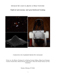
Figure 1: A typical Hertzsprung-Russell/temperature-luminosity diagram; each dot represents a single
star. Valuable information on a star’s evolutionary state can be derived from its position within the diagram
(picture taken from NASAexplore.com).
Star clusters belong to the most important objects in the Universe. First of all, they are
the fundamental building blocks of galaxies, because it is nowadays believed that most, if
not all, stars are born in such groups of a few dozen up to several million stars. Hence,
nearly all stars in galaxies have once been member of a cluster. That makes it crucial for
our understanding of galaxy formation and galactic stellar populations to investigate these
objects in detail.
Moreover, star clusters are unique test beds for stellar-evolution theories. Their most important property, that all member stars were born in a single star-burst out of one giant
molecular cloud, enables us with a few simple observations to get a snap-shot of stellar
evolution of a whole population of stars at a certain age, distance and metallicity. Without
star clusters our knowledge on stellar evolution wouldn’t be nearly as detailed as it is today.
The other way round, observations of star clusters offer the possibility to easily derive
their ages, distances and metallicites by comparing the observations to theoretical stellarpopulation models of certain compositions and evolutionary stages. This latter application
is the main objective of the underlying lab-course project.
For this purpose, the Hertzsprung-Russel diagram (HRD, Fig. 1) can be used which during
the last century proofed to be the optimal tool for studying stellar populations and stellar
evolution. Main objective of this lab-course project is therefore the understanding, preparation and analysis of a color-magnitude diagram (CMD), which is a direct derivative of the
HRD.
1
Advanced Lab Course
Photometry of Star Clusters
This script is organized as follows:
• Section 2 gives an introduction to the subject of this project, i.e. star clusters and the
color-magnitude diagram.
• Section 3 introduces the basic concepts of astronomical observations as well as the
techniques and instruments you will use in this project.
• Section 4 covers the observations you will take out, how you prepare them properly
and how to carry them out such that you can get valueable data.
• Section 5 is about the data reduction of your images and how you extract the information you need from the images.
• Section 6 is the main scientific part where you will be guided through the analysis of
your data.
• The appendix will help you with the Theli software package which you will use during
this project.
Please read all sections (except the appendices) carefully before you start. Make sure you
answered all questions in the text, since you are not allowed to start the project before
answering all questions.
2
Advanced Lab Course
2
2.1
Photometry of Star Clusters
Basic Knowledge of Star Clusters and CMDs
Star Clusters
Figure 2: Picture of the giant molecular cloud Barnard 68 which is relatively nearby, with a distance of
about 200 pc and a diameter of about 0.2 pc. The cloud can only be seen indirectly in optical wavelengths
as it hardly emits light whereas it absorbs all light coming from background sources. It is not known exactly
how molecular clouds like Barnard 68 form, but it is known that these clouds are themselves likely places for
new stars to form. In fact, Barnard 68 itself has recently been found likely to collapse and form a new star
system (picture from the FORS Team with the 8.2-meter VLT, ESO).
Star clusters play a key role in the development of our understanding of the Universe. But
what exactly is a star cluster? In principle any agglomeration of more than a few stars may
be called like this, where “a few” is not well specified and may be taken to be around ten.
In terms of star-cluster dynamics, since the constituent stars mutually attract each other
by the force of gravity, a star cluster may also be defined as a dynamically bound system of
a number of stars.
The fundamental property of a star cluster is its origin, which is assumed to be a single
giant molecular cloud for all members of one cluster (Fig. 2). The according formation
scenario of star clusters is quite well understood nowadays: a collapsing cloud fragments
into small clumps which form the progenitors of the cluster stars. Depending on the size
of the molecular cloud and on the conditions of its collapse, a fraction of about 10-30% of
the gas is consumed by star formation (Adams & Myers, 2001; Lada & Lada, 2003; Allen
et al., 2007). The masses of the stars produced thereby follow a more or less universal
distribution function, which is a quite simple power-law: the so-called initial mass function
(e.g. Salpeter 1955; Kroupa 2001). An important feature of the initial mass function (IMF)
is that it predicts a large number of low-mass and just a few very massive stars (Fig. 3).
3
Advanced Lab Course
Photometry of Star Clusters
Figure 3: Logarithmic representation of the canonical IMF, ξ (solid histogram). The histogram gives the
probability ξ of forming a star of mass m in a star cluster. Between 0.08 M and 0.5 M the IMF has the
slope -1.35. For higher stellar masses it has a slope of -2.35. From this figure it is obvious that it is much
more likely to form low-mass stars than high-mass stars. Figure taken from Kroupa (2001).
T2.1:
The canonical IMF, ξ(m), has the form:
ξ (m) = 0.237 m−1.35
for
m ≤ 0.5 M ,
(1)
−2.35
for
m > 0.5 M ,
(2)
ξ (m) = 0.114 m
which is normalized such that the integral over ξ from m = 0.08 M to m = 150 M is equal
to 1. If you draw 1000000 stars from this IMF, say for the simulation of a globular cluster,
how many will be below 0.5 M ? How much mass will be in stars below 0.5 M ?
When the first newly formed stars ignite, the cluster will still be embedded in its birth
gas cloud. If the initial cloud was rich there will be a couple of large, so-called, O- and
B-stars with masses of up to 150 M , where this upper mass limit is still wildly discussed
(Kroupa, 2005). As can be seen in Fig. 4, these luminous stars will soon blow out the leftover gas and free the cluster from its birth cradle with their enormous radiation pressure
and as a cause of ongoing supernovae.
What is left is an ensemble of stars which is more or less tightly bound, strongly depending
on the initial conditions and the birth parameters. If the initial gas loss is too violent the
cluster will dissolve within a short time, otherwise it will virialise within a few million years
and from then on dissolve slowly (Boily & Kroupa, 2003a,b).
Moreover, based on observations of pre-main-sequence stars, a primordial (i.e. initial) binary fraction of about 100% has been found (Kroupa, 1995) which means that almost every
clump in the collapsing gas cloud splits into two subclumps and in the end yields two distinct stars which form a binary system. The actual value of the binary fraction of observed
clusters is still a debated topic, though. Due to insufficient spatial resolution this question
cannot be answered directly by observations yet, hence uncertainties are still quite large.
The binary fraction of all stars in the Milky Way is believed to be about 50%, i.e., every
4
Advanced Lab Course
Photometry of Star Clusters
Figure 4: Two young star clusters. On the left NGC602, a star forming region, where the massive stars
in the centre already started to blow out the gas. On the right the centre of the Pleiades cluster, which is
about one hundred million years old and exhibits almost no more gas (pictures taken from NASA and the
STScI).
second star on the sky has a companion which in most cases cannot be seen with the naked
eye, while relatively young clusters like the Pleiades (Fig. 4) and Hyades show fractions of
about 60-70% (Kroupa, 1995).
T2.2:
The binary fraction of a star cluster, fbin , is defined as
fbin =
Nbin
,
Ns + Nbin
(3)
where Nbin is the number of binary systems whereas Ns is the number of single stars. Imagine you observe a star cluster and you detect 1000 point sources but you know the cluster
has a binary fraction of 0.7, how many stars are in this cluster?
2.2
Open Clusters vs. Globular Clusters
Historically, star clusters are split up into two distinct populations: open clusters and globular clusters. Although these two families of stellar groups exhibit significant differences
(see Table 2.2), the definitions (as many other things in astronomy) are not strict and there
is even a number of objects (like the cluster Westerlund I) that cannot be clearly assigned
to one of the two.
Open clusters present the lower mass range of star clusters. They assemble from a dozen
up to several thousand stars in a region with a diameter of 1-10 pc. Hence densities vary
significantly from cluster to cluster and reach from about 0.1 M pc−3 (which may rather
5
Advanced Lab Course
Photometry of Star Clusters
Figure 5: The colliding galaxies NGC4038 and NGC4039, also known as the Antennae galaxies. During
this merger of two gas-rich spiral galaxies thousands of star clusters have formed and are still being formed.
Actually, the bright blue points in this Hubble view are not single stars or star clusters but clusters of star
clusters. Credit: Brad Whitmore (STScI) and NASA.
be called associations than clusters) up to 103 M pc−3 .
Globular clusters on the other hand are rich clusters with 104 to 107 stars and diameters of 20 to 150 pc. Unlike open clusters, which are often asymmetric and less centrally
concentrated, these systems are quite smooth and spherical. They furthermore show a very
high concentration in the core which extends from 0.3 up to 10 pc. Typical densities of
these core regions are 104 M pc−3 , thus lie clearly above open clusters and even represent
one of the densest stellar environments in the Universe.
In addition to their different dimensions and shapes the two species of clusters show other
fundamental differences. Taking a closer look at pictures of open and globular clusters in
the Milky Way immediately shows that the former in many cases have diffuse emission from
gas while the later do not. Also, open clusters show bright blue stars which are young and
massive, while they are completely missing in globular clusters.
From the location of the turn-off point in the Hertzsprung-Russell diagram the age of a
cluster can be derived quite accurately. The ages of open clusters found in this way range
from a few million years up to about 10 billion years while globular clusters may have solely
formed about 11-13 billion years ago - at least this is true for most of the known globular
6
Advanced Lab Course
Photometry of Star Clusters
Figure 6: The globular cluster ω Centauri is the largest known cluster in the Milky Way. It is about 50 pc
in diameter and consists of about 10 million stars. On the right is a close-up of the innermost region of ω
Centauri, observed with the Hubble Space Telescope (pictures taken from the Digitized Sky Survey, NASA
and the STScI).
clusters of the Milky Way and other galaxies. However, as mentioned above, there are some
young luminous clusters that resemble in size and mass a globular cluster.
Despite some exceptions, the two groups therefore seemed to be of completely different
origin. Open clusters form continuously, while globular clusters came into existence when
the Universe was much younger and thus denser. Actually, globular clusters are even some
of the oldest objects in the Universe and therefore put a strong limit on the age of the Universe, but also on the understanding of stellar evolution and on structure formation after
the Big Bang.
Another hint for a fundamental difference of their origin was seen in the distribution of
the two types of clusters in the Milky Way and other spiral galaxies as for example Andromeda. Globular clusters are randomly distributed in the halo of the host galaxy and
follow random orbits while open clusters are solely found in the galactic disk.
All this was explained by taking their different formation processes into account:
• As mentioned above open clusters form in the disk, as this is the only place where
enough material can assemble to induce star formation. After birth the newly formed
cluster still moves around the galactic centre in the plane of the disk, just as the birth
cloud has done before.
• In contrast, the majority of globular clusters may have formed while larger structures
as the Milky Way have not existed yet, hence do not have to share the rotation of the
final galactic disk of their host galaxy. Some of the globular clusters may have even
7
Advanced Lab Course
Open clusters
Globular clusters
Photometry of Star Clusters
Abundance
104
102
No. of stars
101 − 104
104 − 106
Diameter [pc]
100 − 101
101 − 102
Age [yr]
106 − 1010
1010
Table 1: Rough overview of the basic paramters of open and globular clusters. Abundance gives the
estimated number of clusters in the Milky Way.
been captured by their host galaxy during merger events (for further details see for
example Binney & Merrifield 1998).
The modern picture interprets both families of clusters as the low-mass and high-mass part
of the same initial cluster mass function (ICMF), which, similar to the IMF, is a power-law.
Observations of star-burst galaxies like the Antennae galaxies (Fig. 5) show that in one
star-formation event clusters of all masses are formed, of course, depending on the available
material and the local star formation rate (SFR). That is, globular-clusters-like objects can
only form in rich molecular clouds with a high SFR - conditions which especially existed
in the very early Universe or during the merging of two spiral galaxies (Kroupa & Boily,
2002). Today in the Milky Way, as in most spiral galaxies, star formation is restricted to
the Galactic disk since this is the only place where enough gas can accumulate to induce
gravitational collapse.
The Milky Way exhibits 150 to 200 globular clusters with typically 105 stars. Open clusters
are more frequent as they are produced continuously, so there are about 1000 known in the
Milky Way. But since they all lie in the Galactic plane most of them are heavily obscured
by dust. The total number of open clusters in the Milky Way therefore is supposed to be
about 20000.
Probably the most famous open cluster of the Milky Way is the Pleiades Cluster, which
is a typical galactic cluster with about 1000 stars, a diameter of approximately 10 pc and
an age of about 125 million years. The Pleiades can be well seen with the naked eye due its
small distance of roughly 135 pc and the bright heavy stars in its centre (see Fig. 4).
By far the most massive cluster of the Milky Way is ω Centauri (Fig. 6) with more than 10
million stars and a diameter of about 50 pc. With its enormous mass, ω Centauri represents
the upper mass limit of a star cluster, therefore may also be classified as an ultra compact
dwarf galaxy or the nucleus of a stripped dwarf spheroidal galaxy (e.g. Fellhauer & Kroupa
2003). In addition, recent observations show that it is indeed much more complex than a
regular star cluster since its temperature-luminosity diagram shows pronounced substructure, i.e., ω Centauri may consist of more than one stellar population (Hilker et al., 2004).
T2.3:
Calculate the angular size of:
• a typical globular cluster in the halo (50 pc diameter at a distance of 10 kpc),
• a typical open cluster in the disk (5 pc diameter at a distance of 1 kpc),
• the full Moon (10−10 pc diameter at a distance of 10−11 kpc).
8
Advanced Lab Course
2.3
Photometry of Star Clusters
HRD/CMD
In 1913 Henry Norris Russell presented his recent work at a meeting of the Royal Astronomical Society. There he showed a diagram that represented a relation between the spectral
classes and the absolute magnitudes of all stars for which fairly reliable distances had been
obtained so far (Russell, 1913). Soon the importance of this discovery became clear to the
astrophysical community and since then the so-called Hertzsprung-Russell diagram (Ejnar
Hertzsprung was the first to anticipate the existence of a relation between the two quantities) has given a great contribution to the understanding of stellar evolution.
Hitherto, much effort has been put into this specific type of diagram and it was found that it
is possible to replace spectral class on the abscissa by temperature and absolute magnitude
on the ordinate by the star’s luminosity to obtain a similar diagram: the temperatureluminosity, or color-magnitude diagram (Fig. 1). The advantage of the latter lies in the
way the corresponding quantities can be obtained. While it is rather hard to determine
the spectral class of a star, it is much easier to obtain its temperature in means of a color
index. So, just by taking pictures of a star cluster with two different color filters the temperature/color and the apparent luminosity/magnitude can be derived and a color-magnitude
diagram (CMD) can be drawn. How this is done will be subject of this lab-course project.
The evolution of stars within a CMD has been widely studied and is a major subject of
every basic astronomy training. The most common classifications of stellar objects like
main-sequence star, red giant, white dwarf, etc., are derived from this type of diagram and
are taken to be well-known by the students carrying out this lab-course project. An advanced overview on stellar evolution can be found in Binney & Merrifield (1998), p. 258,
or, more detailed, in de Boer & Seggewiss (2008).
2.4
Colors & Magnitudes
To understand the various flux measurements we make with our telescope setting, we have to
clearify first which quantities exactly we measure and how we can derive physical quantities
out of them. Here we introduce you to the basic principles you need for carrying out this
project, a more complete picture is given in Binney & Merrifield (1998), p. 26.
2.4.1
Apparent Magnitude
The apparent magnitude, m, is a measure of a star’s brightness as seen by an observer on
Earth. In other words, it is the integrated radiation flux, f , measured in W/m2 contained in
a particular frequency range, ∆ν. Measuring fluxes of celestial bodies in different frequency
ranges is called astronomical photometry which is the main objective of this lab-course
project.
Based on a magnitude system first introduced by ancient Greek astronomers, the apparent
magnitude is a comparative scale in which brighter stars are given smaller magnitudes than
fainter stars, such that
f1
m1 − m2 = −2.5 log10
,
(4)
f2
9
Advanced Lab Course
Photometry of Star Clusters
where the indices denote the magnitudes and fluxes of two distinct stars.
But there is extinction of radiation through intergalactic gas, interstellar gas and, of course,
through the earth’s atmosphere. In addition, there’s also flux getting lost in our telescope.
Thus, the flux which reaches the solar system is not the flux which was emitted by the
source and the flux received by our detector, f , is not the flux fν that reaches the solar
system. While former varies from source to source, the latter is fixed and can be quantified
for any instrument. We measure
f≡
Z ∞
fν Tν Fν Rν dν,
(5)
0
where Tν is the transmission of the atmosphere, Fν is the transmission of any applied filter
and Rν is the efficiency of the telescope system.
Depending on the frequency range, there is significant extinction due to the Earth’s atmosphere, Tν . The amount of extinction furthermore depends on the column density of
air along the line of sight and increases with lower observing angles. Therefore, the best
possible observing conditions are achieved near the zenith, where the length of the light
path through the atmosphere is minimal. Extinction and disturbing seeing effects get worse
for observations at lower elevations. These effects are often expressed in terms of the objects airmass a, which tells you through how much atmosphere (column density) the light
travels compared to vertical in-fall. For an angular distance z from the zenith it can in good
approximation be computed as a = 1/ cos z such that a = 1 for an object at the zenith and
formally a = inf at the horizon.
The filter transmission Fν is readily determined for well defined filters like the Johnson
filters which will be used in this lab course (Sec. 2.4.5). The instrumental efficiency Rν is
a composite of the efficiency of the telescope’s optical system and the sensitivity of the CCD.
In order to get well defined magnitudes of star-cluster members for a color-magnitude diagram we can correct the observed fluxes of the stars by observing a reference star which
is nearby the cluster and whose magnitudes in different frequency ranges/filters are well
known, since the observing conditions (air mass, filter, telescope optics, CCD) for such a
reference star are approximately the same as for the cluster. By measuring f for the reference star as well as for the cluster stars and by knowing the magnitude of the reference
star, we can obtain the magnitudes of the cluster stars using equation 4.
Note: the flux of a single star is mostly determined by fitting a two-dimensional Gaussian distribution to the CCD image. This Gaussian results from the point-like appearance
of the star which gets convolved with the telescope point-spread function (PSF). By integrating over this distribution function the total flux, f , of the star can be determined and
converted to magnitudes as described above. In contrast to stars, galaxies and star clusters
often appear as extended sources on the CCD. Their magnitude is determined by fitting
appropriate distribution functions to the CCD image and integrating over these functions
out to a pre-defined cut-off radius. In this way it is possible to define magnitudes for extended sources, but these values have to be handled with care as there are always underlying
models which have been assumed and which may differ significantly from case to case.
10
Advanced Lab Course
Photometry of Star Clusters
T2.4: You observe a reference star and measure 16000 counts, from the literature you
know that this star has an apparent magnitude of 15.0. For a second object you measure
4000 counts. What is the apparent magnitude of this object?
2.4.2
Distance Modulus
The observed flux f of an object depends not only on its intrinsic brightness but also on
its distance, d. In fact, the flux decreases with d−2 . If we want to calculate the flux F of a
certain object assuming that it was at distance D we can therefore use
f=
D
d
2
F.
(6)
In this context, the absolute magnitude M is defined as the apparent magnitude an object
would have if it was located at some standard distance D, where this distance is always
taken to be 10 pc. Using equation 4 we then get
m − M = −2.5 log10
f
F
= 5 log10
d
D
= 5 log10 d − 5,
(7)
where the quantity (m − M ) is called the distance modulus of the specific object. Hence,
by knowing m and d we can correct the apparent magnitude for the non-standard distance.
On the other hand, if we know m and M we can infer the distance d.
T2.5: From the literature you know that the abolute magnitude of your object from T2.4
is M = 10 mag. What is the distance of the object, and what is the distance modulus?
2.4.3
Interstellar Extinction
Absorption and scattering of photons in the interstellar medium can cause stars to appear
dimmer than they actually are. This effect is called interstellar extinction and has to be
handled with care. If we have A magnitudes of extinction then equation 7 has to be rewritten
as
m − M = 5 log10 d − 5 + A.
(8)
Fortunately, interstellar extinction is, unlike the distance effect, strongly wavelength dependent such that it can be measured by taking images in multiple color filters. For many
objects reliable extinction measurements are therfore available
T2.6: How does the distance of your object from T2.4 change in the case you have 0.2
mag of extinction?
11
Advanced Lab Course
2.4.4
Photometry of Star Clusters
Metallicities
In astronomy all chemical elements heavier than He are called metals. In the first few minutes
after the Big Bang just a very low percentage of all baryons was synthesized to metals while
most baryons synthesized to hydrogen and helium. In fact, accurate primordial abundances
have already been predicted by Alpher, Bethe & Gamow (1948) out of theoretical Big-Bang
nucleosynthesis considerations before first accurate measurements were made. The standard
values which are assumed for primordial abundances in most stellar-evolution calculations
are X = 0.765 for hydrogen, Y = 0.235 for helium and Z = 0 for metals.
Through stellar evolution, the metallicity in the Universe increases as hydrogen and helium are processed into heavier elements. Nuclear fusion in stars in combination with stellar
winds and supernova explosions permanently enriches the interstellar material. The solar
metallicity, for instance, is about Z = 0.02, hence it has formed out of already enriched
gas. Stars which form out of enriched material evolve differently from metal-poor stars as
the metal content has a large influence on stellar evolution and the stellar structure. For
instance, higher metalicities cause stars to become dimmer and cooler below a stellar mass
of about 4 M . Above this mass, an increase in Z only causes a decrease in a star’s temperature.
For a single star, this metallicity effect can only be taken into account by taking deep
spectra and fitting theoretical models of stellar atmospheres to the observed spectra. Since
all stars in a star cluster have the same Z, the metallicity of a cluster can be determined from
a CMD by fitting various stellar-evolution models with a range of metallicities to the data
and using the fact of the mass-dependent reddening and dimming of stars with increasing
metallicity. Unfortunately, the precission of the underlying data has to be very high for this
method. Due to the rather bad seeing conditions in Bonn we will refer in this experiment
to literature values.
T2.7: Draw two schematic CMDs in one plot, one of a globular cluster with an age of 11
Gyr and a metallicity of Z = 0.001, and the other of an open cluster with an age of 100
Myr and Z = 0.02. Include the main sequence, the giant branch and the horizontal branch
(if applicable) in your sketch.
2.4.5
Johnson-Filter System
The most commonly used photometric system is the UBV-system based on the work by
Johnson & Morgan (1953). The acronym stands for ultraviolet, blue and visual and denotes
the wavelength coverage of the three most-often used filters. Meanwhile, this system has
been extended to the infrared with the filters R (red), I (infrared) and then J, H, K, L and M
(for an overview of the corresponding wavelengths and filter characteristics see for example
Binney & Merrifield 1998, p. 53). For the lab-course project the Johnson filters U, B, V, I
and R are available (Fig. 7).
Note: Nowadays, the Johnson-filter system is being replaced in many applications by the
Sloan-filter set (Fukugita et al., 1996) which has a similar wavelength coverage (u’, g’, r’,
12
Advanced Lab Course
Photometry of Star Clusters
Figure 7: The transmission functions of the five available Johnson filters (picture taken from the University
of Göttingen).
Figure 8: The transmission functions of the five Sloan filters (picture taken from Fukugita et al. 1996).
i’, z’) but allows a higher transmission in each filter (Fig. 8) and therefore requires shorter
exposure times. Due to this varity of available filters, conversions of observed fluxes into
apparent magnitudes have to be done carefully. It is crucial that the measured fluxes of the
reference stars in a given filter are compared to the listed magnitudes of the reference stars
in the specific filter, i.e. if you observe with Johnson filters make sure the magnitudes of the
reference stars you use are listed in the Johnson system and not in Sloan or anything else.
The same holds for the theoretical isochrones which you fit to your data.
13
Advanced Lab Course
3
Photometry of Star Clusters
Basic Knowledge of Astronomical Observations
Almost all of our astronomical knowledge has been devised from the measurement of electromagnetic waves emitted from various forms of matter (e.g. stars, molecular clouds, etc.) in
the universe. Due to the large distances from these emitters to us, the intensity of radiation
we can measure is very small, thus sensitive equipments are needed. Nowadays for optical
observations like the one you will do, radiation (photons) is collected and imaged by an
optical telescope and detected (converted into electronic signal) by a CCD detector. This
section tends to give you a basic introduction to the equipments you will use, and what you
need to do to produce scientific data.
3.1
Telescope optics
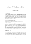
Figure 9: Light path in a Cassegrain reflector telescope. The red star indicates the Cassegrain focus where
the CCD camera should be placed.
The telescope used for this lab course is a 50 cm Cassegrain reflector telescope placed in the
dome on top of Argelander-Institut für Astronomie, Bonn. It has an f-number (f-ratio) of
f/9 at its Cassegrain focus and f/3 at its primary focus. We will use the telescope here only
in the Cassegrain focus.
T3.1:
3.2
Calculate the focal length of the telescope in both foci.
CCD detector
CCDs (Charged coupled devices) are now widely used as photon detectors, both in the
largest astronomical optical telescopes and in your pocket digital camera. A CCD detector
consists of a two-dimensional array of picture elements (pixels), which are produced as a
light-sensitive metal oxide semiconductor (MOS) capacitor on a silicon substrate. CCDs
make use of the inner photoelectric effect to convert the distribution of photons to the distribution of electrons, which are then collected in capacitors and sequently read out: after
an exposure is terminated, the collected charge is shifted column by column to a readout
column by an alternating voltage impressed on the picture elements. The readout column
is finally read out pixel-wise and the resulting signal amplified and converted to a digital
signal by an analogue digital converter.
14
Advanced Lab Course
Photometry of Star Clusters
As a detector, a CCD has the advantages of:
• high sensitivity (high quantum efficiency of up to 90%),
• high dynamical range (the limits of luminance range that a detector can capture),
• linearity over almost the entire dynamical range,
• large spectral range (mid-infrared to ultraviolet for optical-optimised detectors),
• direct availability for further computer aided data analysis.
A less advantageous property of CCDs is the so-called dark current. At room temperature dark current brings CCD pixels to their saturation level within a minute or even less.
Therefore astronomical CCDs are always cooled. Cooling is done thermo-electrically (temperature difference to ambient temperature: about 30◦ C), with closed cycle systems or by
liquid nitrogen (CCD temperature can reach -100◦ C).
The CCD camera in use for the lab course is of type SBIG STL-6303E, which has 3072
× 2048 pixels, where the size of each pixel is 9 µm × 9 µm. It has a Full Well Capacity
of 100000 e− , i.e. in each pixel it can store 100000 electrons, and an ADU (Analog To
Digital Converter Unit) gain of 1.4 e− /ADU. It can be thermo-electrically cooled to about
30◦ below room temperature.
T3.2: Calculate the field-of-view (FOV) of the telescope and the theoretical angular resolution. What limits the angular resolution during your observations?
3.3
Observational conditions and requirements
There are some undesirable yet existing effects which will hinder you from getting good
data if you don’t take care of them correctly. Here we list those of them which will be
encountered in this lab course. The treatment of these effects during data reduction will be
done rather automatically using sophisticated software.
3.3.1
Seeing
The light distribution of a point source (e.g. a star) on the image plane is called point spread
function (PSF). In the idealised case, a PSF is determined by the telescope aperture. With
a normal circular aperture with diameter D, it is an Airy disc with an angular resolution of
∆θ = 1.22
λ
D
(9)
where λ is the wave-length of incoming light. However, when the blurring effect of earth’s
atomosphere is taken into account, the actual resolution is much worse for ground-based
telescopes. And the PSF can be better described by a two-dimensional Gaussian. The size
of such a stellar image can be described by the full width at half maximum (FWHM) of
the Gaussian, which is called the seeing of the image. Naturally seeing measures the actual
15
Advanced Lab Course
Photometry of Star Clusters
resolution in a particular observation, and it reflects the stability of Earth’s atmosphere on
a given night at a given location as seen through the telescope. The best seeing on the
surface of earth is about 0.4”. It’s found at high-altitude observatories on small islands such
as Mauna Kea or La Palma. For the condition above AIfA Bonn, a 2” seeing is already good.
To measure the seeing on your image, you can choose a non-saturated star and measure
its FWHM in number of pixels using the telescope software, and then convert it to arcseconds using the relation:
pixel size/µm
× 206 = 00 /pixel
(10)
focal length/µm
The pixel size of the CCD and focal length of the telescope can be found in the above
subsections.
T3.3:
Derive the factor 206 in equation 10.
3.3.2
Focusing
If the CCD camera is out of focus you will get a big blob for each star on your image. So,
before taking science frames, make sure you have the right focus by adjusting the focus until
you get the sharpest image.
3.3.3
Linearity, saturation, dynamical range and exposure time
When speaking about linearity, “linear” means the increase in measured signal is propotional to the increase in the incoming photon flux. It is a desired property of the detector
since it enables a direct measurement of the incoming photon flux. A CCD detector has
good linearity over almost the entire dynamical range, but only over the dynamical range.
When the detector reaches the saturation level, it is no longer possible to derive the exact
number of photons that reached the detector originally. Therefore it is very important not
to saturate the objects of interest by a too long exposure time. For bright stars a few seconds’ exposure suffices to reach saturation. On the other hand one needs a long exposure to
detect weak sources. And the longer the exposure
√ time, T , is, the larger the signal to noise
ratio (remember that S/N is proportional to 1/ T ). The selection of exposure time is thus
dependent on the specific scientific goal of the observation. Only if a large number of objects
of interest is not saturated, photometric analysis and calibration are possible. Thus, better
make many shorter exposures of your object and co-add the images (see next section).
T3.4: For a standard star of magnitude m1 = 3.0 you get 30000 counts after an exposure
time of t1 = 10s. How long do you have to make an exposure for a star of magnitude
m2 = 5.0 to get the same number of counts?
16
Advanced Lab Course
3.3.4
Photometry of Star Clusters
Cosmics and dithering
Two more artifacts will influence the quality of your data: “dead” pixels on the detector and
cosmic rays. The former results to that, several pixels on each of your obtained images only
represent noise but not any signal. The latter, on the other hand, leads to the saturation
of several pixels around the cosmic ray impact position. While the number and positions of
the dead pixels are fixed, the number of cosmic rays depends on the exposure time and their
positions are random. These artifacts will hinder you from getting information on those
pixels which correspond to certain positions on the sky. To avoid totally losing information
at those positions, several frames (6 is suggested here) are taken of each scientific object and
the telescope is moved slightly between each exposure. This method is called “dithering”.
The multiple frames are then aligned and the median of each pixel of the combined image
is determined, with the consequence that all extreme values are discarded. This method
also has the advantage that the signal to noise ratio is improved without saturating brighter
sources.
3.4
3.4.1
Image Reduction Steps
BIAS subtraction
The signal of the CCD is first converted from an analog count signal (electrons in the pixel,
i.e. a voltage value) into a digital number by an analog-digital converter. For example,
with a 16 bit analog-digital converter you would transform your analog voltage values from
the pixels into 216 = 65536 discrete levels, i.e. each pixel would get a value between 0 and
65535. For a better coverage of the available range of counts the logarithm of the analog
signal is taken first. This is because you want to be very accurate for pixels with only a
few counts but do not need to be that accurate for pixels with many counts. But, since
the analog-digital converter can only handle positive values and fails for a value of zero, an
offset has to be added electronically to every pixel value during the read-out process before
the logarithm is taken. Otherwise, small voltages would lead to negative numbers thus
would make the converter give out high positive values as the next value below 0 is 65535
in the example of a 16 bit converter. This so-called BIAS has to be recorded by a zero-time
exposure called the BIAS frame, which then has to be subtracted from every image as the
first step of data reduction.
3.4.2
Dark current subtraction
Even if the CCD chip is NOT exposed to optical light, there will still be a current flowing
in it due to thermal fluctuations, which is called the dark current. Dark current is one of
the main sources for noise in image sensors such as a CCD. The pattern of different dark
currents in the pixels across the CCD can result in a fixed-pattern noise. Taking DARK
frames and subtract them from the science (and FLAT) frames can remove an estimate of
the mean fixed pattern, but there still remains a temporal noise, due to the fact that the
dark current itself has a shot noise.
Note that the level of dark current is strongly dependent on the temperature of the CCD
chip and the length of the exposure. For a liquid nitrogen cooled CCD camera, the dark
current can be neglected for many observational purposes. But in this lab course it has to
17
Advanced Lab Course
Photometry of Star Clusters
be taken into account. Thus, you should also make sure that the CCD temperature and
exposure time for the DARK frames match those of the light (science) frames.
3.4.3
Flat fielding
You also need to take some FLAT frames by making exposures towards a uniformly illuminated background (e.g. twilight sky or a carefully constructed and illuminated dome flat
field screen, currently we use the former). However, your obtained image will be far from
uniform. On your FLAT frame you will probably see “donuts” which represent dust grains
somewhere within the light path, and other variations of light due to the telescope optics.
Also, the response of the CCD is not exactly the same from pixel to pixel, such pixel-wise
variation is also recorded in a FLAT frame. The exposure time for the FLAT frames should
be determined such that the peak brightness level of a FLAT frame is 1/2 or 2/3 of the
saturation level ( saturation = full well in e− /ADU gain). And for each filter used for science exposures, a new FLAT frame should be made. This is because the pixel response
to incoming light is wave-length dependent. During data reduction a FLAT frame will be
normalized to an average value of 1 and used to divide the science image.
T3.5:
What can you infer from the sizes of the donuts?
T3.6:
How many counts do you expect your FLAT frames to have?
3.4.4
Masking/weighting
When one pixel on your CCD is more sensitive to another one (which always happens),
you would like to trust the sensitive one more since it gives you data with higher S/N.
This can be done by assign individual weights for every pixel, a process called weighting.
The weighting factors can directly be taken from the normalised FLAT. Weighting is also
neccessary when you try to co-add frames (see co-adding): your object on each frame may
be at different positions (usually the case, see dithering), when co-adding them, a proper
weighting ensures maximised S/N in the final image.
For those bad pixels/columns on the CCD chip and cosmic rays, a simple way of treatment is to “mask” them using softwares and assign them less weight. There are two types
of masks: global and individual. One global mask is made for a particular CCD detector
and can be applied to all images produced by it. One can also create an individual mask
for each image, counting also for cosmic rays.
3.4.5
Astrometric calibration
Your obtained image is a telescope-configuration-dependent projection of a curved sky. Thus
the pixel/detector coordinates and the sky coordinates do not have a simple relation. To
project your image back onto the sky coordinates is called astrometric calibration. This can
also be done by softwares, with the help of a reference catalogue.
18
Advanced Lab Course
3.4.6
Photometry of Star Clusters
Sky subtraction
During exposures the CCD not only collects light from your target of interest, but also
receives radiation from the background sky. In addition there will be ADU counts from
unresolved objects and glow from objects not even in your field of view (e.g. a bright star
nearby, or the moon!). By determining this background level and removing it from your
image, only the source flux will remain. The usual way of modelling the background is to
first remove all objects in your frame and then smooth the image with a specific kernel
width. Then this background image can be subtracted from the original frame.
3.4.7
Co-adding
By stacking all science images into one and making sure that each object falls onto the same
pixel, the final image will have a higher S/N value than each image alone. This process is
called co-adding.
3.5
Photometric calibration, reference stars
For the same star on the sky, observations through different telescopes under different
weather conditions will observe different fluxes. Converted to magnitudes, you get a particular instrumental magnitude which does not directly reflect the true magnitude of the star.
The most simplistic ansatz is to assume you only have an offset Z between your observed
magnitudes and the true ones.
mcalib = minstr + Z
(11)
So you can calibrate your instrumental magnitudes by observing some reference stars or
“standard stars” whose calibrated magnitudes are well known and stable. Observe such
stars using the same configurations as your scientific objects. For this lab course project it
is sufficient to look up the magnitudes in the different filters for some reference stars in your
chosen clusters from a catalogue, or compare it to a well calibrated CMD of this cluster
from the literature and add appropriate offsets.
19
Advanced Lab Course
4
Photometry of Star Clusters
Observations
After reading this section you are supposed to know what you need to do during your nighttime observations, step by step. Furthermore, by reading this section you should choose
your objects to be qualified for the observations. Feel free to discuss with your tutors if you
have questions.
The data files you should obtain during your observations are:
• 10 FLATs in each of the 2 filters (B and V),
• 10 BIAS frames,
• 6 science exposures in each of the 2 filters for each object,
4.1
Choosing Your Objects
As a first exercise, choose yourselves the two star clusters (one open cluster and one globular cluster) to observe from the short list provided below. Your choice should base on the
“visibility” of the objects during the night of observations, i.e. their tracks across the sky.
It would be desirable to have the object as high (in altitude) as possible during the time
of observations. One other factor to take into account is the position of the moon. You
wouldn’t like to have your object to be close to a full moon since a bright moon would
significantly increase the level of your sky background and thus decrease the signal-to-noise
ratio (S/N) of your object.
One convenient way to visualize the tracks of the objects during one night is to produce a
visibility plot. Make one yourself according to the instructions in the task below, figure out
its meaning, and choose your objects basing on it.
T4.1:
Generate a visibility plot for the date of your observation. Procede as follows:
• go to http://catserver.ing.iac.es/staralt/ ,
• select mode: Staralt; Date: your expected date for observation,
• specify the coordinate of AIFA, Bonn: 07 04 01 50 43 46 [75],
• load the file(s) containing the object coordinates provided by your tutor,
• include “Moon distance” in “Options”,
• generate one plot for open clusters and one for globular clusters.
Which direction does the peak of one object track correspond to?
T4.2:
Pick two objects (one OC and one GC) according to your visibility plots.
20
Advanced Lab Course
Catalog Name
M103 (NGC 581)
M36 (NGC 1960)
M50 (NGC 2323)
M11 (NGC 6705)
M29 (NGC 6913)
Photometry of Star Clusters
RA
01:33:23
05:36:18
07:02:42
18:51:05
20:23:57
DEC
+60:39:00
+34:08:24
-08:23:00
-06:16:12
+38:30:30
mv
7.4
6.0
5.9
5.8
6.6
dim [’]
5
10
14
13
10
Table 2: List of Open Clusters. The first column gives the Messier and/or New
General Catalogue (NGC) catalog name of the star cluster. RA is the Right Ascension
of the star cluster for epoch 2000 (hour:minute:second), while DEC is the Declination
of the star cluster for epoch 2000 (degree:minute:second). mv gives the cluster’s
total (integrated) visual magnitude and the last column gives its angular diameter in
arcminutes.
Catalog Name
NGC 288
NGC 2419
M 3 (NGC 5272)
M 92 (NGC 6341)
M 15 (NGC 7078)
RA
00:52:47.5
07:38:08.5
13:42:11.2
17:17:07.3
21:29:58.3
DEC
-26:35:24
+38:52:55
+28:22:32
+43:08:11
+12:10:01
mv
8.1
10.4
6.2
6.4
6.2
dim [’]
13
5
18
14
18
Table 3: List of Globular Clusters. Columns are the same as for Tab. 4.1.
4.2
Observing Schedule
Since time is short during the night every step has to be planned in advance. Therefore, an
observing schedule has to be prepared beforehand. For details on the tasks which have to
be performed during the night see the observer’s manual at the telescope.
1. Telescope and CCD camera setup.
2. Cool down the CCD to about 25 degrees below the current temperature.
3. FLAT frames (10 FLATs/filter). Note that there’s very limited time in which a SKY
FLAT (FLAT frame towards evening/morning twilight sky) can be taken. So prepare
everything beforehand and hurry up!
4. Focusing
5. Science frames of your objects
6 science frames/object, apply dithering in between.
reference/standard star (if not in the same frame with the object)
6. BIAS and DARK frames (10 each). They can be taken at any time during the night.
The exposure time of DARK frames should be the same with the science frames.
Note: depending on the telescope software it may be possible to automatically take
DARK and BIAS frames with each exposure and automatically subtract them from
the science frames. This may be convenient but is not always recommendable.
21
Advanced Lab Course
4.3
Photometry of Star Clusters
Data storage
Since you will take a number of frames during the night it is recommended to create an
appropriate tree folder on the local hard drive of the telescope beforehand. The data reduction software Theli requires a certain folder structure which you should stick to from the
very beginning to avoid confusion. This structure looks as follows:
• The top folder name should have your names and the date of observations in it, e.g.
XunShi AndreasKüpper 20091224/
• There should be a separate folder for any BIAS frames, e.g.
XunShi AndreasKüpper 20091224/BIAS/
• If you take DARK frames, then you also need a separate folder, e.g.
XunShi AndreasKüpper 20091224/DARK/
• Each set of FLAT frames for a specific filter should have a separate folder, e.g.
XunShi AndreasKüpper 20091224/FLAT B/
XunShi AndreasKüpper 20091224/FLAT V/
• Each set of science frames for a specific object and filter gets its own folder, e.g.
XunShi AndreasKüpper 20091224/M92 B/
XunShi AndreasKüpper 20091224/M92 V/
Also name your files properly, otherwise you will get confused on the next day or whenever
you work with the data again.
22
Advanced Lab Course
5
Photometry of Star Clusters
Data Reduction
For reducing the data and extracting a catalogue of sources out of the pictures, a number of
steps are necessary and a variety of scripts and programmes will be used. In this section we
will introduce the tools you need for creating a color-magnitude diagram, this will be done
in the order in which you will have to use them.
5.1
ALADIN
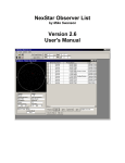
Figure 10: Main window (left) and server selector window (right) of Aladin.
Before starting any work on the data, make sure you know how your object looks like.
Therefore, start Aladin, a virtual telescope in which you can view parts of the sky in allsky catalogues like the Sloan Digital Sky Survey or 2MASS (if Aladin is not installed on
your computer, Skycat can do the same, see next section). Open a terminal window and
type
> aladin
and the Aladin window will show up (Fig. 10). Aladin enables you to access a variety of
survey data. For our purposes an all-sky catalogue with a good coverage of the northern
hemisphere is recommended. To select, for example, one of the servers of the Digitized
Sky Survey (DSS) go to File/Load astronomical image/DSS and choose one of the available
locations. The server selector window will show up (Fig. 10). Enter the name of your target
into the appropriate box, e.g. M92, and select a survey from the Sky Survey drop-down
menu, e.g. DSS2-blue. Also make sure that the requested field-of-view is at least as large
as the FOV of your telescope. After pushing SUBMIT the data will be received from the
server and displayed in the main window. Additionally, the coordinates of the object will
be given at the top of the window.
23
Advanced Lab Course
Photometry of Star Clusters
Figure 11: Main windows of Skycat (left) and DS9 (right).
5.2
SKYCAT/DS9
You can check your own images and compare them with the virtual-telescope data by using
Skycat or DS9. For the first one type
> skycat
in a terminal window. Open any image with the menu File/Open and select the the file you
want to open. To adjust the view of the image push the button Auto Set Cut Levels first
and then go to the View/Colors menu. In the new window you can choose various color
scalings, color maps and intensity functions. Pick for example Linear, heat and gamma for a
good representation of your star cluster (Fig. 11). With Skycat you can also access on-line
catalogues like DSS. Simply choose an appropriate catalogue from the Data-Servers menu.
DS9 is similar to Skycat but offers slightly different functionality. To start DS9 type
> ds9
in a terminal window and the DS9 window will show up (Fig. 11). As in Skycat, open any
file with the File/Open menu. The scaling of the view can be adjusted via the Scale and
the Color menu. Choose, for example, Square Root, 99.5% and Grey. You can now easily
adjust the scaling by holding the right mouse button and moving the cursor up and down
or left and right.
5.3
THELI
The data reduction itself will be done with Theli, a freely-available software package for
the reduction of astronomical imaging data which was in part developed at AIfA1 . An introduction to Theli is given in the appendix of this document, therefore we only give the
necessary steps here but strongly recommend going through the appendix first.
Before you start working on your data make sure you have made a backup of the whole
data set. Also ensure that all files are stored in appropriate folders as described in Sec. 4.
1
http://www.astro.uni-bonn.de/~mischa/theli.html
24
Advanced Lab Course
Photometry of Star Clusters
Figure 12: The initialise window of Theli.
Throughout the reduction we recommend to follow the processing of your files by checking
the specific folder content after each reduction step and following the renaming of the files.
This might be very helpful in case a reduction step fails or has to be redone or undone.
Note that Theli is not fail safe and needs the caution of the user. Note also that not all
reduction steps have to be repeated for each filter, e.g. BIAS processing, and might even
lead to errors when repeated.
Start Theli by typing
> theli
in a terminal window and the main window will show up which has seven panels which have
to be gone through from left to right. Thus, in the following sections we will go through
each of the seven panels in the correct order.
25
Advanced Lab Course
Photometry of Star Clusters
Figure 13: The preparation window of Theli.
5.3.1
Initialise
In the initialise window of Theli enter an appropriate name for the data set you are reducing into the “Current LOG file” line, a new log file will be created. Start with one filter and
don’t start reducing a second filter set before you finish the first. Just to make sure that no
old preferences are set, hit the “Reset” button next to the LineEdit afterwards.
For the given filter enter the directory names into the appropriate lines. Make sure the
“Main path” is an absolute path and not a relative one, i.e. that it gives the full path
starting from root.
Finally, before proceeding to the next panel, choose the camera you used from the instrument list.
26
Advanced Lab Course
Photometry of Star Clusters
Figure 14: The calibration window of Theli.
5.3.2
Preparation
In the preparation window you have to check the “Split FITS / correct header” box and hit
the “Start” button. Note that this task has to be done for the BIAS and DARK frames just
once as they are used for all filters. If you go through this task for a second set of pictures
for a different filter make sure that you remove the specific lines from the “Commands”
window before hitting the “Start” button.
5.3.3
Calibration
In the calibration window first check the “Process biases / darks” box and then hit “Start”.
Note again, that this task also has to be done just once, for the other filters simply skip this
step.
Then check “Process flats” and start the procedure.
27
Advanced Lab Course
Photometry of Star Clusters
Figure 15: The weighting window of Theli.
Finally, you have to calibrate your data. Therefore, check also the “Use DARK” box (for
those cases where you need a dark current subtraction, i.e. long exposures) but not the
“Create SUPERFLAT” box before you push the start button.
5.3.4
Superflatting
Superflatting will not be applied in this lab course project.
5.3.5
Weighting
In the weighting window you have to start the “Create global weights” process and then the
“Create WEIGHTs” process.
28
Advanced Lab Course
Photometry of Star Clusters
Figure 16: The astrom / photometry window of Theli.
5.3.6
Astrom / Photom
The Astrom / Photom window of Theli contains essential steps of the data reduction process of your data which have to be done with care. First of all, get the coordiantes of your
object, e.g. from Aladin, and enter them in to the RA and DEC fields. Make sure that
you use the same coordinates for all filters!
Then you have to download an astrometric reference catalog. Therefore, select “Web (CDS)”
and “USNO-B1” (catalog from photographic plates) or “2MASS” (catalog from a digital survey). Make sure the radius of your requested catalog covers a few arcsec more than your
field-of-view, choose an appropriate magnitude limit (e.g. 15) and hit “Get catalog”. The
larger your radius and the fainter the limiting magnitude, the more sources you will get in
your catalogue. Don’t have too many sources in this catalogue as the astrometric solution
will get less accurate with more such degrees of freedom.
Check the “Create source cat” box and push the “Configure” button. In the create source
29
Advanced Lab Course
Photometry of Star Clusters
Figure 17: The create source catalogue window (left) and the astrometry configuration
window (right) of Theli.
catalog window (Fig. 17) set the DETECT THRESH and the DETECT MINAREA parameters to one of the following values: (5,5), (10,10), (40,15) or (100,20). Begin with the
lowest numbers and switch to a higher set in case Theli finds no astrometric solution in
the following reduction step. For very noisy data with a low S/N ratio you can try (1,5)
first. Also you can increase the “Minimum FWHM” to 4 pixels as it is very unlikely that
you will get a better seeing than that. Close the configuration window by pushing “Ok”
and hit “Start”.
Finally, make the astrometric and photometric solution. Therefore, check “Astro + photometry”, select “Scamp” from the drop-down menu and enter the “Configure” menu.
In the astrometry configuration window (Fig. 17) and try the following values: POSANGLE MAXERR 5, POSITION MAXERR 5, DISTORT DEGREES 1. Press “Ok” to exit
this window and start the process. If Theli finds no astrometric solution try creating a
new source catalog with different parameters as stated above or change the two MAXERR
parameters to about 10.
5.3.7
Coaddition
In the coaddition window (Fig. 18) first start the sky subtraction by checking the corresponding box and pushing the “Start” button. Then check the “Coaddition” box and enter
the “Configure” menu. In the configuration window (Fig. 19) enter the coordinates which
you also entered in the previous reduction steps. Furthermore, enter an identification string
into the specifc box. The name should be clear, e.g. blue, green, red or B, V, R. Furthermore, enter the pixel scale of the CCD, i.e. 0.4 (in some cases the quality of the extracted
30
Advanced Lab Course
Photometry of Star Clusters
Figure 18: The coaddition window of Theli.
magnitudes can improve when you choose 0.8 here). Exit the configuration menu and start
the coaddition.
After this step you are done with the given filter. Proceed with the reduction of the next
filter before you go to the next section. After finishing all available filters you should make
a new folder, e.g.
XunShi AndreasKüpper 20091224/M92 FINAL/
and copy all the coadded pictures and their weights into this folder.
5.3.8
Prepare color picture
After the reduction of the images you have to make sure that all pictures cover the same
field. This is usually not the case. Therefore we crop the borders of the images such that
all images have the same size and show the same part of the sky. This can be easily done
with the “Prepare color picture” routine of Theli which you find in the top bar under
“Miscellaneous”.
31
Advanced Lab Course
Photometry of Star Clusters
Figure 19: The coaddition setup window of Theli.
In the “Create color picture” window (Fig. 20) write the location of your folder with the
coadded images (created in the previous reduction step) and hit “Get coadded images”.
Remove all images from the list which are not necessary and crop the images by pushing
the “Crop maximum overlap” button.
If this step was successful your are done with the data reduction with Theli. The next step
will be to extract the final source catalog from the coadded and cropped images. This will
be done with SExtractor in the next section.
But before proceeding with the next step you can create a color picture of your object
if you have managed to take images in three filters. Therefore go to the “Color calibration”
tab of the “Create color picture” window and select the three images in the drop down
menus at the top (Fig. 21). First try to let Theli create the color picture automatically by
pushing “Calibrate” and then “Preview”. If the colors of the final picture are not according
to your taste hit the “Reset” button and try to adjust the weighting factors for the three
colors by hand. The result will be stored in preview.tif in your current working directory.
5.4
SExtractor
The final extraction of the sources will be done using SExtractor2 , a program that builds
a catalogue of objects from an astronomical image. Although it is particularly oriented
towards reduction of large scale galaxy-survey data, it can perform reasonably well on moderately crowded star fields. Thus, it may lead to bad results in the centres of globular
2
http://www.astromatic.net/software/sextractor
32
Advanced Lab Course
Photometry of Star Clusters
Figure 20: The create color picture window of Theli.
clusters, but will suffice for our purposes.
Here, we will extract the sources with a small home-made shell script that makes use of
the SExtractor routines. Therefore, create a folder, e.g.
XunShi AndreasKüpper 20091224/M92 CATALOGUE/
and copy the following files into this directory:
• get catalogue.sh,
• get catalogue.assoc,
• get catalogue.makessc,
• the cropped images,
• the cropped weights.
Run the script by typing the following command in a terminal window:
> get catalogue $PATH $B $V $R
where $PATH is the full path of the current folder, $B is the name of the blue cropped image, $V is the green cropped image and $R is the third, in case you have made observations
in a third filter. Otherwise simply repeat argument $V, in this way you will get an “R”
column in the catalogue which is redundant, since it repeats the magnitude of the V-band.
The script will create source catalogues, just as was done in Theli, for each filter and
cross reference the three catalogues. Only sources which get detected in all three filters will
be written to the resulting ascii catalogue which will be located in
33
Advanced Lab Course
Photometry of Star Clusters
Figure 21: The create color preview window of Theli.
XunShi AndreasKüpper 20091224/M92 CATALOGUE/result/result ascii.cat
where the columns are:
1. right ascension (J2000) in degrees,
2. declination (J2000) in degrees,
3. B magnitude,
4. V magnitude,
5. R magnitude.
You additionally get catalogues for each filter and the combined catalogue in an enhanced
file format (LDAC) comparable to the .fits format for images, which you don’t need here
any more, but which you should keep in mind in case you ever need to deal with more
sophisticated catalogues.
You can quickly count the number of detected sources by typing
> wc -l result ascii.cat
within the result directory. The number of detections depends on the parameters DETECT MINAREA and DETECT THRESH just like we used them in Theli. You can set
those parameters by editing the script with a text editor or by simply adding the two numbers to the command line argument:
> get catalogue $PATH $B $V $R $DETECT MINAREA $DETECT THRESH
where you should choose one of the pairs (5,5), (10,10), (15,40) or (20,100). You can play
with the values and compare the resulting numbers of detections. The larger values will give
34
Advanced Lab Course
Photometry of Star Clusters
you less false detections but also much less sources. You have to decide, which detections
you will base your analysis on.
35
Advanced Lab Course
6
Photometry of Star Clusters
Analysis
After extracting the catalogue from the observational data you can begin the analysis. Aim
of the analysis will be to determine the most basic parameters of the clusters, the distance
and age. We recommend to do the analysis with gnuplot since it is a very convenient tool
for such tasks as plotting data from many different files. For help on the functionality of
gnuplot we recommend some on-line help pages34 .
6.1
Calibration
Begin your analysis by drawing a first color-magnitude diagram. Therefore start gnuplot
in a terminal window by typing
> gnuplot
Plot the color index B-V versus the V magnitude with the following command
> plot ’result ascii.cat’ using ($3-$4):($4)
where the $3 and $4 are the columns in the file. Note that the magnitudes in your catalogue
are not calibrated yet. This has to be done by hand, by comparing the measured magnitudes
of a few stars with reference magnitudes of on-line archive data and applying a correction
constant to each magnitude. You can do that, for example, with
> plot ’result ascii.cat’ using ($3+0.3-$4+0.1):($4+0.1)
For the calibration of the magnitudes you will either use the magnitudes of the reference
stars which you have observed seperately or your tutor will provide you with the reference
magnitudes of some (non-variable) stars in your field-of-view. For the latter, identify the
reference stars in your catalogue by their right ascension and declination and calculate the
correction constant for each filter. If the quality of your data does not allow for this method
your tutor will provide you with a literature CMD of this specific cluster such that you
can shift your magnitudes accordingly. Now you can draw a calibrated CMD. What is the
limiting magnitude of your observations?
6.2
Extinction
Extinction by interstellar dust makes stars appear dimmer than they are. This can be
corrected for by adding a constant factor to each magnitude. In principle these factors
can be determined through a color-color diagram in which two color indices are plotted
versus each other. But therefore you need reliable images in three colors and sophisticated
analyses. This is hardly possible with the data taken from Bonn due to light pollution, thus
we will stick to values listed in the literature. Often the extinction factor is smaller than
the achievable accuracy in magnitudes which can be achieved from Bonn. Thus, assume an
extinction factor, E(B-V), of zero, if not stated otherwise by your tutor.
6.3
Distance Determination
The distance to star clusters can be determined in different ways, e.g. with variable stars
or supernovae. With our CMD we can also derive the distance since there are stars in each
cluster with well defined absolute magnitudes. By comparing the observed magnitudes of
those stars with their theoretical absolute magnitudes we can evaluate the distance modulus
3
4
http://www.gnuplot.info/faq/faq.html
http://t16web.lanl.gov/Kawano/gnuplot/index-e.html
36
Advanced Lab Course
Photometry of Star Clusters
Figure 22: Isochrones for high and low metallicity stellar populations. The main sequence
of young clusters is almost independent of metallicity for B − V < 0. For old clusters (older
than 109 yr) the horizontal branch is independently of metallicity located at +0.5.
of the cluster. But the stellar populations of open clusters and globular clusters can differ
significantly, such that not every method can be applied to every cluster.
6.3.1
Main-Sequence Fitting
From Fig. 22 we can see that open clusters of young age have a well defined main sequence
for high mass stars, which does not vary significantly with metallicity. Based on this part of
the main sequence we can estimate the distance without regard to the age and metallicity
of the cluster. Therefore take the youngest isochrone of one of the isochrone directories, e.g.
isochrones/geneva/008/iso c008 0600.UBVRIJHKLM
and plot column 9 (B-V) versus column 7 (absolute V magnitude) into your open cluster
CMD, i.e.
> plot ’result ascii.cat’ using ($3+0.3-$4+0.1):($4+0.1),
’∼/SCPHOT/geneva/008/iso c008 0600.UBVRIJHKLM’ using ($9):($7) with line
Apply a constant shift to the V magnitudes such that the high mass part of the main
sequence fits the observations. From this shift you can calculate the distance d by using
d = 100.2(m−M +5) pc.
37
(12)
Advanced Lab Course
6.3.2
Photometry of Star Clusters
Position of the Horizontal Branch
Old globular clusters do not show an extended main sequence (Fig. 22). But, as stellar
populations evolve, massive stars move onto the horizontal branch where they burn helium
in the core. The absolute magnitude at which they shine in this stage is well known and
can be used to determine the distance to old star clusters.
MV of horizontal branch stars is approximately +0.5 mag. Thus, identify the horizontal
branch in your CMD, shift your V magnitudes accordingly and apply equation 12.
6.4
Isochrone Fitting
After we have produced a well calibrated CMD we can fit a theoretical isochrone to the
data and see which parameters reproduce the cluster best. For this task we use the Geneva
database of isochrones (Lejeune & Schaerer, 2001), named after the university of origin.
Note that these isochrones are based on simplified assumptions and that they obey an intrinsic uncertainty. There are other databases of isochrones, coming, e.g., from Padova
(Nasi et al., 2008), which in some cases differ substantially from the Geneva models. For
simplicity we stick to the Geneva database here.
The available set of isochrones covers metallicities of Z = {0.001, 0.004, 0.008, 0.020, 0.040, 0.1}
and ages of 103 yr to 15 Gyr in a reasonable step width. The data is stored in the folder
geneva. This folder contains subfolders for each metallicity and in every subfolder are separate files for each age. For example the file
geneva/001/iso c001 0950.UBVRIJHKLM
contains the isochrone for Z = 0.001 and for an age of 109.5 yr. The columns in the files
are always the same. Use column 9 for B-V and column 7 for the absolute V magnitude.
For each cluster go through the data set and compare the theoretical isochrones with your
data. For young clusters you should stick to high metallicities whereas for old clusters you
should apply low metallicities.
When you have a good fit, you can change the output to a file instead of the screen and
give an output name. Afterwards you must change to the screen again, though:
> set terminal eps postscript enhanced
> set output ’figure1.eps’
> plot ’result ascii.cat’ using ($3-$4):($4),
’∼/SCPHOT/geneva/008/...’ using ($9):($7) with line
> set terminal x11
Our aim is it to understand anything in our CMD, since there should be an explaination
for any position of any data point in the graph. Therefore, answer the following questions:
• What age has the specific cluster?
• How large are the uncertainties in this determination? How can you estimate reasonable uncertainties?
• What influences the width of the main sequence, i.e. why is the main sequence not as
thin as the isochrone predicts? Think about how the isochrone is produced, and what
is assumed in this process.
38
Advanced Lab Course
Photometry of Star Clusters
• Can you identify stars that lie beyond the turn-off point, i.e. are bluer than the turn-off
point but still appear to lie on the main sequence? How can this happen?
• How many stars can you identify in this way to appear abnormal in age/color and
what does it tell you about the stellar population of this cluster?
Do this for all clusters for which you have taken data and for each additional catalogue
which your tutor hands out to you.
39
Advanced Lab Course
Photometry of Star Clusters
Figure 23: The two main GUI elements: the menu bar (top) and the tabbed menu.
A
THELI user manual – lab-course short version
General description of the GUI and its elements
Main elements and nomenclature
The main window (Fig. 23) consists of two main parts:
• a menu bar at the top of the window and
• a dialogue with a tabbed menu.
We will refer to the seven tab menues of the latter as processing groups (PG for short).
These are
• Initialise
• Preparation
• Calibration
• Superflatting
• Weighting
• Astrom / Photom
• Coaddition
and contain the various reduction steps or other settings. The data is reduced by making
some initial settings in the first processing group (tell the software where the data is, which
instrument was used, etc.), and then one works his way through the remaining six PGs.
40
Advanced Lab Course
Photometry of Star Clusters
Figure 24: A tooltip appears whenever you hover with the cursor over certain GUI elements.
Integrated Help system
Besides the help described here, see also the troubleshooting section in App. A.9.
A very extensive help layer has been integrated that comes in various active and passive
forms.
• On the lowest level there are simple tool tips that are displayed when you hover with
your mouse button over a specific PushButton or other element unless the meaning of
those is obvious (see. Fig. 24).
• More extensive help for the various PGs and reduction steps is available under Help
→ What’s this?. The cursor will change to a question mark. Move it anywhere into a
GroupBox with the reduction steps to obtain general information of what is happening
in this particular PG. Or click on the CheckBox of a particular reduction step to obtain
more detailed information for this task, such as if this step is mandatory or optional,
and if you have to provide any parameters.
• The Help menu provides you with further support, such as dialogue containing an
overview of the functionality of the various GUI elements. Furthermore, you can
access this document as well, the general pipeline documentation or a rather technical
paper analysing the performance of THELI .
• If the GUI expects some parameters as input it will highlight the according fields for
you with a red background colour etc. The colour coding is explained in detail in the
following subsection.
• Each reduction step you run dumps all programme and script output into the SCRIPTLOG. You can access these, for each PG separately, through View → Processing logs
in the menu bar.
A.1
A.1.1
The INITIALISE processing group
Pipeline Settings
The LOG file The four PushButtons and the first LineEdit are associated with the LOG.
Say, you start working on a new R-band data set of NGC 1234, then NGC1234 R would
41
Advanced Lab Course
Photometry of Star Clusters
Figure 25: The Initialise PG
qualify as a nice LOG name. Enter it in the corresponding LineEdit, then click on the
Clear processing status PushButton. This will flush the GUI from all settings that might
be left over from a previous reduction run. Parameters in the GUI and the LOG are set
to meaningful default values. If the LOG entered does not yet exist, it is created at this
moment. It is automatically updated (or created, if not yet existing) if you switch to any
other PG, or shut down the GUI. The LOG will contain all reduction steps, parameter and
GUI settings you have done or chosen for a particular data set. Choose a new LOG name
if you reduce a different data set. If you leave this field empty and start processing anyway,
the LOG will be named noname.
Whenever you launch THELI , it will read the LOG that was used last, updates all GUI
elements and internal variables correspondingly and switches to the PG that was active
when you closed your last THELI session. You can continue with your reduction at the
point where you left it the last time.
LOGs are usually stored in ∼/.qt/ and linked to ∼/.theli/reduction logs/. The previous path may vary depending on your Qt installation. You will never have to touch a LOG
file, apart from loading an old one into the GUI.
42
Advanced Lab Course
Photometry of Star Clusters
Clear Clears the processing status in the LOG, and resets all GUI elements to default
values. This is useful if you want to start again with your data reduction from the very
beginning, or start with an entirely new data set.
A.1.2
Data directories
The LineEdit fields collected in this GroupBox tell THELI where the data is that you
want to process. You specify the main directory path (hereafter: maindir ) that contains
everything, followed by the names of the subdirectories that contain the BIASes, FLATs
etc. Behind each subdirectory you will find the number of images that was found in the
corresponding place. (Note that these numbers may not correspond to the actual number
of images in the corresponding directory, due to an un-solvable bug in THELI !) All fields
do not accept blank characters as input, in addition the subdirectories do not accept a slash
(/). You only need to specify those subdirectories which you actually need.
Restore ORIG This deletes all data in the corresponding directory, apart from the
very raw data that has been moved into the ORIGINALS subdirectory. The ORIGINALS data
is played back, thus restoring the original state before any processing has been launched. If
no ORIGINALS subdirectory is present, nothing will be deleted.
Clear dirs
A.2
A.2.1
Clears all LineEdits.
The PREPARATION processing group
Split FITS / correct header
The main job of this task is to split multi-extension FITS files into single chips, thus allowing
for parallel processing. It also writes a new FITS header conformed with the THELI pipeline.
If single-chip images are given, only the FITS header will be updated.
This reduction step will be applied automatically to all subdirectories that are specified
in the Initialise PG.
How to redo the task Delete all split images in the corresponding directories, and move
back the images from the ORIGINALS directory.
A.3
A.3.1
The CALIBRATION processing group
Process biases / darks
Combines all BIASes in the BIAS subdirectory set in the Initialise PG. You can override
this by entering a different subdirectory in the LineEdit next to the CheckBox. The more
BIASes you have the better your master BIAS will be and the smaller the calibration noise
that is introduced into your SCIENCE images. We recommend to use at least 10 BIASes.
Overscans are corrected and trimmed.
How to redo the task Delete the BIAS i.fits images from the BIAS dir and rerun.
They have to be deleted because otherwise they are taken as an input image.
43
Advanced Lab Course
Photometry of Star Clusters
Figure 26: The Preparation PG.
A.3.2
Process flats (MANDATORY)
Combines all FLATs in the FLAT subdirectory. Again, you can override this by entering
a different subdirectory. A FLAT correction is very useful even if the camera appears to
be illuminated very homogeneously. This is because the FLAT does not only correct for
vignetting effects, but also for different sensitivities on a pixel-to-pixel basis. The more
FLATs you have, the better the master FLAT will be and the smaller the calibration noise
you introduce into your SCIENCE images. We recommend at least 10 FLAT exposures.
The FLAT exposures are debiased, overscan corrected and scaled to the highest mode in
the stack before combination.
How to redo the task Delete the FLAT i.fits images from the FLAT dir and rerun.
They have to be deleted because otherwise they are taken as an input image.
A.3.3
Calibrate data
Images are overscan corrected, debiased and flat fielded. If suitable, a SUPERFLAT is calculated from the data as well.
44
Advanced Lab Course
Photometry of Star Clusters
Figure 27: The Calibration PG.
If you decide to calculate a SUPERFLAT from this data, then activate the Calculate SUPERFLAT CheckBox. The parameter configuration dialogue appears. Alternatively, you
can bring it up with the Configure PushButton.
Superflat parameters Here you determine how objects in the images are detected, and
which method is used for image combination. The left field takes the detection threshold
(DT) per pixel, given in units of sigma of the sky background noise. The middle field takes
the minimum number of connected pixels (DMIN) above DT which make up an object. The
smaller both values are, the fainter the objects you mask. The right field accepts the size
of the convolution kernel for the sky background. Its effect is very minor at this stage and
you do not have to worry too much about it. A good starting point for optical data is
(1.0|5|250), depending on the flatness of the image and the detector size.
If your images exhibit strong fringing, then you can no longer use very low detection thresholds, since then the fringes themselves are detected as objects and thus removed from the
SUPERFLAT. In this case one can no longer calculate a fringing model from the SUPERFLAT. We recommend to use a high S/N threshold if strong fringing is present. Try starting
with (5.0|5|250) in this case. With near-IR detectors DT and DMIN often must be increased
to 10 in order to not mask features in the very inhomogeneous sky background. If one or
45
Advanced Lab Course
Photometry of Star Clusters
Figure 28: Configuration for the outlier rejection during image stacking, and the creation
of a SUPERFLAT.
more of those three LineEdits is left empty, then the default values will be used without
warning.
You can choose between a median and a mean combination for the SUPERFLAT. The
median delivers a more stable result for a small number of stacked images, whereas the
mean has lower noise when more images are stacked.
How to redo the task Delete the OFC images in SCIENCE and play back the previous
exposures from the SCIENCE/SPLIT IMAGES directory. Images in SCIENCE/SUB IMAGES are
overwritten.
A.4
A.4.1
The SUPERFLATTING processing group
Smooth SUPERFLAT, create fringe model
This step smoothes the SUPERFLAT that was created previously, yielding an illumination
correction that can be used to superflat the data. The difference between the smoothed
and the unsmoothed SUPERFLAT gives the fringing model. The illumination correc46
Advanced Lab Course
Photometry of Star Clusters
Figure 29: The Superflatting PG.
tion images are called SCIENCE i illum.fits, whereas the fringing models are named
SCIENCE i fringe.fits.
How to redo the task
A.4.2
Just rerun. Previous results will be overwritten.
Superflatting
This step superflats your data by dividing each frame by the illumination correction.
How to redo the task Delete the OFCS images in SCIENCE and move back the images
in SCIENCE/OFC IMAGES.
A.4.3
Defringing
If you want to defringe your data, you must have superflatted your data previously by
a smoothed SUPERFLAT (= the illumination correction). This task scales the fringing
models according to the sky background of your exposures in relation to the SUPERFLAT,
and then subtracts the rescaled fringe model.
47
Advanced Lab Course
Photometry of Star Clusters
Figure 30: The Weighting PG.
How to redo the task Delete the OFCSF images in SCIENCE and move back the images
in SCIENCE/OFCS IMAGES.
A.5
A.5.1
The WEIGHTING processing group
Create globalweights
The normalised FLAT is taken and has bad pixels replaced by zero values. Whether a pixel
is bad is determined by one or more threshold pairs which refer to the normalised FLAT
itself.
How to redo the task
A.5.2
Just rerun.
Create WEIGHTS
All cosmics, hot pixels and other chip defects are detected on an image by image basis in
this step.
How to redo the task
Just rerun.
48
Advanced Lab Course
Photometry of Star Clusters
Figure 31: The Astrom / Photom PG.
A.6
A.6.1
The ASTROM / PHOTOM processing group
Astrometric reference catalogue
Retrieving a catalogue from the web This is the default state. You can select the
GSC2, the USNO-B1 or the 2MASS as a database. The catalogue will be retrieved from
CDS and is reformatted for use with THELI .
You can control the limiting magnitude of the objects retrieved (in the catalogue’s magnitude system), and therefore their number density. The catalogue will be retrieved around
the reference coordinates within the radius specified. The coordinates themselves can be
entered in decimal or hexagesimal values. If left empty, they will automatically be determined from the current data set. You retrieve the catalogue by clicking on the Get catalog
PushButton. The GUI will not accept any other input during the time it takes to get the
catalogue (seconds to minutes). It appears frozen, but it is not (will change in the future).
Once downloaded and processed, the message window will tell you how many sources it got
from the catserver at CDS. You may then rerun the task with a modified limiting magnitude
if you are not happy (too few or too many objects).
49
Advanced Lab Course
Photometry of Star Clusters
Figure 32: Configuration for the catalogue creation.
How to redo the task
is retrieved.
A.6.2
Old results will be overwritten when a new reference catalogue
Create source cat
Here we extract source catalogues from all images. The detection characteristics can be
fine-tuned by means of the configuration dialogue (Fig. 32).
Parameter configuration DETECT THRESH is the detection threshold (in sigma of
the sky background noise), and DETECT MINAREA is the minimum number of connected
pixels above that threshold. The latter depends on the seeing and the pixel scale of your
instrument. Three more parameters that usually do not need to be modified, are available,
too (Fig. 32).
If you leave a field empty, then the default value will be used. No warning message will be
printed.
General tips for the catalogue creation The WEIGHT maps created previously are
taken into account in the catalogue creation process, guaranteeing a clean catalogue that is
largely free from spurious detections.
50
Advanced Lab Course
Photometry of Star Clusters
Figure 33: Configuration dialogue for Scamp
If the image quality is good you can have both DETECT THRESH and DETECT MINAREA
as low as (5|5). If you have many hundreds or thousands of sources in an image, then choose
a higher pair of thresholds, such as (10|10) or (40|15), or even (100|20). THELI has been
used successfully with the latter parameters even for extremely crowded fields such as the
Magellanic Clouds or exposures taken near the galactic centre.
The object catalogues created are saved in SCIENCE/cat/.
How to redo the task
A.6.3
Just rerun. Old catalogues in SCIENCE/cat will be overwritten.
Astro+photometry
Here you can choose between three methods: Scamp, Astrometrix and Shift only. The latter determines only relative astrometric offsets and relative photometric zeropoints. It does
51
Advanced Lab Course
Photometry of Star Clusters
not care for sky position angles or absolute sky coordinates. It can not handle mosaicing
and only works for single-chip data. It requires a reasonable overlap of sources between
exposures. This method is most useful if you work with images that show just one or a few
objects. It serves as a fall-back solution if the other two solutions fail (for whatever reason).
Scamp (usually fast) and Astrometrix (usually slower) on the other hand are the entire
opposite. They calculate the linear offsets between the reference pixel (CRPIX) and the
reference coordinates (CRVAL), as well as two-dimensional distortion polynomials of higher
order. There is no difference in running them on a single-chip or on a multi-chip camera.
In the latter case, the solution is for the entire mosaic.
The results of the astrometry step, regardless of the method chosen, will be written to
a headers subdirectory inside SCIENCE.
Configuration We recommend to use Scamp for this experiment. You can run it in its
default configuration, with one small modification: the degree of the distortion polynomial
should be set to 2 (instead of 3) as there are not many sources in our data that can be used
for distortion correction. All other parameters can be left unchanged.
How to redo the task
A.7
A.7.1
Just rerun. Old results in SCIENCE/headers will be overwritten.
The COADDITION processing group
Sky subtraction
Configuration This step subtracts objects above certain user-provided thresholds from
the image. From the remaining sky an estimate is determined. The Configure dialog
(Fig. 35) presents you with the following options [lab-course: here we present only the
option we are going to use]
Automatic sky modelling In a first pass, SExtractor is run to remove all objects from
the image. The result is then smoothed and subtracted. To this end you must provide the
usual detection threshold, minimum number of connected pixels, and the extent (pixels) of
the smoothing kernel. This is the default method and useful for all exposures where the
largest object is significantly smaller than the field of view of the detector.
How to redo the task
A.7.2
Just rerun. Old results will be overwritten.
Coaddition
The coaddition goes in three steps. First, global information about the data set is obtained,
and the reduction settings are made accordingly. Then, the SCIENCE images and their
associated WEIGHTs are resampled. Lastly, the resampled images are combined.
52
Advanced Lab Course
Photometry of Star Clusters
Figure 34: The Coaddition PG.
A.8
Guidelines for observers using THELI
Do this
• When acquiring your data, orient the camera such that its axes are parallel to the
right ascension and declination axes. THELI prefers North up and East left, but will
handle any orientation of 0, 90, 180 and 270 degrees, including flips. The coadded
image will always exactly have North up and East left.
• When planning your observations, make sure that you dither your exposures (apply
small telescope offsets after each image).
Do not do this
• Do not reduce different data sets in parallel, especially from different filters. This leads
only to confusion, and you might use up your disk space sooner. Finish one reduction
and then go to the next data set.
• You currently can not run two instances of THELI at the same time, since both of
them will overwrite each others parameter and configuration files. You can do this
53
Advanced Lab Course
Photometry of Star Clusters
Figure 35: The configuration window for manual sky subtraction
safely if you have two separate installations in two different paths, owned by two
different users, and having THELI launched by these two users.
A.9
FAQ and Troubleshooting
General
Q: I want to activate the CheckBox of some reduction task, but the according command
does not appear in the command window. What am I doing wrong?
A: You forgot to provide either a necessary parameter (look for a red LineEdit field), or you
did not specify all necessary directories in the Initialise PG. For example, you might have
forgotten or misspelled the BIAS directory. Whenever a command does not appear, then
information is missing.
Q: Bother! The GUI crashed/hung up while a reduction task was running! What do I
have to do now?
A: Probably NOTHING, apart from relaunch. The GUI will come up in the same configuration it had when it died. Besides, the GUI is just a graphical engine, it does nothing else
than launching reduction processes. Those are running stand-alone without supervision by
the GUI. If the GUI crashes then this has no effect on the job running. Just see top to learn
when the job has finished, then bring up a new instance of the GUI. Besides, a crash of the
GUI should happen very rarely only.
54
Advanced Lab Course
Photometry of Star Clusters
Figure 36: The dialogue for obtaining image statistics.
Calibration
Q: During the pre-processing steps in the Calibration and Superflatting PGs my computer
gets horribly slow and sticky. What’s going on?
A: Your machine is swapping. If you work under Linux you can see this in the memory
ProgressBar at the bottom of the window. It becomes red and tells you how much swap space
is currently used. Solaris users don’t see this ProgressBar. Lower the number of images
loaded simultaneously into memory (the NFRAMES parameter in the Initialise PG) such
that they consume not more than about 40% of your physical RAM.
Astrom / Photom
Q: I want to retrieve an astrometric reference catalogue from the web through the orange
window in the Astrom / Photom PG, but no results are returned. What is wrong?
A: Sometimes the CDS server is down. Check the status of your local network as well.
A.10
Image statistics
Calling Image statistics from the Miscellaneous pull-down menu, presents you with the
dialog shown in Fig. 36.
Image directory Specify here the path to the images for which you want to obtain some
statistics.
55
Advanced Lab Course
Photometry of Star Clusters
Name filter This is a string for filtering a subset of images out of all files in the specified
directory. For example, it can simply be something like A*OFCS.fits. If left empty, all
images (*.fits) in the directory will be considered.
How it works Clicking on the Get statistics PushButton will retrieve the statistics. This
can take a while, and the GUI will not allow any other action during this time (may change
in a future release). The table obtained will automatically be stored in the directory you
specified. The name of this file will include the name filter, if such a filter was put. If the
table is obtained a second time with an identical filter, the old file will be overwritten without warning. You can manually save the table to a different file name, or load a previously
created table.
If the Create source cat and Astrometry processing steps were done as well, seeing and
relative photometric zeropoints will be shown as well, respectively. That requires the presence of a cat and / or a headers directory in the specified path.
56
Advanced Lab Course
Photometry of Star Clusters
References
Adams F. C., Myers P. C., 2001, ApJ, 553, 744
Allen L., et al., 2007, prpl.conf, 361
Alpher R. A., Bethe H., Gamow G., 1948, PhysRev, 73, 803
Binney J., Merrifield M., 1998, Galactic Astronomy, Princeton University Press, NJ
Boily C. M., Kroupa P., 2003a, MNRAS, 338, 665
Boily C. M., Kroupa P., 2003b, MNRAS, 338, 673
de Boer K. S., Seggewiss W., 2008, Stars and Stellar Evolution, EDP Sciences, France
Fellhauer M., Kroupa P., 2003, Ap&SS, 284, 643
Fukugita M., Ichikawa T., Gunn J. E., Doi M., 1996, AJ, 111, 1748
Hilker M., Kayser A., Richtler T., Willemsen P., 2004, A&A, 422, L9
Johnson H. L., Morgan W. W., 1953, ApJ, 117, 313
King I. R., 1962, AJ, 67, 471
Kroupa P., 1995, MNRAS, 277, 1491
Kroupa P., 2001, MNRAS, 322, 231
Kroupa P., 2005, Nature, 434, 148
Kroupa P., Boily C. M., 2002, MNRAS, 336, 1188
Lada C. J., Lada E. A., 2003, ARA&A, 41, 57
Lejeune T., Schaerer D., 2001, A&A, 366, 538
Nasi E., Bertelli G., Girardi L., Marigo P., 2008, MmSAI, 79, 738
Russell H. N., 1913, Obs, 36, 324
Salpeter E. E., 1955, ApJ, 121, 161
57