Download Lab memo lab 2 - ISY: Communication Systems

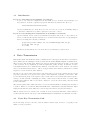
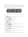
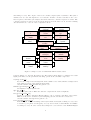
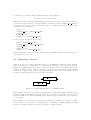
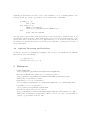
Software-Defined Radio
Lab 2: Data modulation and transmission
Version 0.2
Anton Blad and Mikael Olofsson
November 16, 2012
1
Introduction
In this lab, you will build a transmitter and corresponding receiver for simple DBPSK modulated
data framed with a correlation sequence in the beginning. The receiver prints the estimated SNR
of the received data, as well as the computed bit error rate. You will then modify the transmitter to
include an AWGN channel model and verify that the measured SNR and bit error rate correspond
to the theoretical values. You will further modify the system to use DQPSK modulation instead
of DBPSK.
2
Preparations
Read this memo through. Then determine suitable values of the parameters that are mentioned
in Section 4.2.
3
Setup
The following hardware is needed for this lab:
• A computer with USB 2.0
• A USRP1 with an LFTX/LFRX daughterboard pair at the A side
• An oscilloscope with two channels
You need GNU Radio installed. The lab is tested and ensured to work with GNU Radio 3.3.0,
and assumes that it is installed in /usr/local/gnuradio-3.3.0.
1
3.1
Initialization
If you are doing this lab in CommSys’ research lab:
Log in to one of the lab computers as the user SDR lab user. Your lab teacher will give you
the password. Your lab computer is prepared with all needed files in the directory
/home/sdrlabuser/labfolder/lab2
Open a terminal and cd to that directory. You do not need to worry about making changes
to files there. That directory will be updated for the next occation.
If you are not following these instructions in CommSys’ research lab:
Open a terminal. Create a directory labfolder somewhere and cd into it. If you have done
Lab 1, you should already have that directory. Download and extract the accompanying lab
files by executing the following commands:
$ wget http://www.commsys.isy.liu.se/SDR/labs/gr/lab2.tar.gz
$ tar zxf lab2.tar.gz
$ cd lab2
All files needed in this lab are now in the directory lab2 that you just created.
4
Data Transmission
Full synchronization is assumed in many communications courses given at LiU and at other universities. That is also the assumption in the lectures and tutorials in TSKS01 Digital Communication.
The reason for that is that syncronization provides problems and solutions enough to form a full
course by itself. It is a significant problem in engineering reality, though. In this lab, we have
real signals and there is no artificial syncronization of senders and receivers. Instead, our senders
and receivers must include tricks to achieve an approximate syncronization, which then contains
frequency correction and bit syncronization.
We also need to know where data starts. Our data will be grouped into frames and the sender
prepends each frame by a pseudo-noise sequence that marks the beginning of the frame. The
receiver knows that pseudo-noise sequence, and correlates the received bit-stream by that sequence.
A large correlation marks - with high probability - that we have found the start of a frame. This
is frame syncronization. The receiver then continues to detect the whole frame, and then waits
for the next frame.
The absolute phase will be unknown in the receiver, but will essentially be unchanged from symbol
to symbol. Therefore, we will use differential PSK in the communication systems in this lab. That
simply means that the phase difference between adjacent symbols carry the information.
This is described in more detail below. Details about how and why this kind of syncronization
works is discussed in the follow-up course TSKS04 Digital Communication Continuation Course.
4.1
Noise-Free Transmission Link
In the following, let M be the size of the modulation scheme used, and let k = log2 (M ) be the
number of bits per symbol.
2
The simple data transmitter is shown in Figure 1. It consists of a data source generating a stream
of data vectors that are all equal. Each data vector is framed with a simple correlation sequence
at the beginning, then converted to a stream of bits. The stream of bits is packed to a number
of bits per sample, corresponding to the chosen modulation, then differentially encoded, mapped
to a complex symbol, and then passed through a root-raised-cosine shaping filter. The signal is
finally modulated to the carrier frequency by the USRP.
pr.data_source_counter
src
gr.chunks_to_symbols_bc
symmap
gr.interp_fir_filter_ccf
rrc
pr.framer_simple_vbb
framer
gr.diff_encoder_bb
diffenc
gr.multiply_const_cc
txscale
pyblk.txmeta_decap_b
decap
pr.pvec_to_stream
v2s
usrp.sink_c
u
Figure 1: A transmitter for differential PSK modulated data.
Compare Figure 1 to the stub file psk_tx.py. The blocks perform the following operations in
order:
src (pr.data source counter)
Generate data blocks of known data. The reason that we want to transmit known data is to
give us the possibility to check if the received data is correct.
Uses the variable data size in the python code.
framer (pr.framer simple vbb)
Prepend each data block by a pseudo-noise sequence.
Uses the variables frame size and corrseq in the python code.
decap (pyblk.txmeta decap b)
Remove meta data header from packet.
Uses the variable frame size in the python code.
v2s (pr.pvec to stream)
Convert frames to a stream of bits.
Uses the variable frame size in the python code.
diffenc (gr.diff encoder bb)
Differential encoder. y[n] = (x[n] + y[n − 1]) (mod M ). The result are the symbol indices.
Uses the variable mod order in the python code.
symmap (gr.chunks to symbols bc)
This block maps symbol indices on the actual symbols, which are complex numbers.
Uses the variable constpoints in the python code.
rrc (gr.interp fir filter ccf)
An FIR filter that also upsamples (interpolates) the signal. This is a so-called root-raisedcosine filter, which shapes the signal to increases the spectral roll-off of the modulation.
More about this in TSKS04.
Uses the variables samples per symbol and rrctaps in the python code.
txscale (gr.multiply const cc)
Amplify the signal to fit the USRP signal levels.
u (usrp.sink c)
Send the sampled complex baseband signal to the USRP transmit chain, resulting in the
physical output signal.
Uses the variable usrp interp in the python code.
On the receiver side, the structure is shown in Figure 2. The baseband processing includes an automatic gain control followed by the gr_mpsk_receiver_cc block that does frequency correction
3
and timing recovery. The output of the block contains complex symbol estimates. The symbol
estimates are decoded and unpacked to a bit stream. A frame correlator searches for the correlation sequence, and frame sync samples the frame when the correlation sequence is found. The
correlation sequence is removed, the header is stripped from the data vectors, and the resulting
data stream is fed to a bit error rate computation block.
gr.multiply_const_cc
1
0
symscale
usrp.source_c
rxscale
gr.diff_phasor_cc
agc
gr.mpsk_receiver_cc
diffdec
gr.fir_filter_ccf
recv
rrc
gr.probe_mpsk_snr_c
snrest
sigview
gr.agc_cc
gr.multiply_const_cc
u
pygui.signal_viewer
pr.rate_estimate
gr.constellation_decoder_cb
symrate
constdec
gr.delay
pr.frame_correlator_simple_bb
delay
framecorr
pr.frame_sync_bb
0
1
pr.rate_estimate
pr.pvec_to_stream
datarate
pr.ber_estimate_b
berest
rxv2s
0
1
pr.data_source_counter
refdata
framesync
pr.deframer_simple_vbb
deframe
pyblk.rxframe_decap_b
rxdecap
pr.pvec_to_stream
refv2s
pyblk.txmeta_decap_b
refdecap
Figure 2: Simple receiver for differential PSK modulated data.
Compare Figure 2 to the stub file psk_rx.py. The pink blocks in Figure 2 constitute the actual
signal path. Those blocks perform the following operations in somewhat rough order:
u (usrp.source c)
Receive the complex baseband signal from the USRP receive chain, which is a sampled and
demodulated version of the physical input signal.
Uses the variable usrp decim in the python code.
rxscale (gr.multiply const cc)
An amplifier. Adjust signal levels.
agc (gr.agc cc)
Automatic gain control. Make sure that the output has the desired amplitude.
rrc (gr.fir filter ccf)
Again a root-raised-cosine filter, Matched filter to the root-raised-cosine filter of the sender.
This block allows for decimation (down-sampling) as well, but that is not used here.
Uses the variable rrctaps in the python code.
recv (gr.mpsk receiver cc)
Performs mpsk detection including carrier syncronization and symbol timing recovery. Uses
a Costas loop for phase and frequency recovery and a method called Mueller and Muller
for timing recovery. To some extent, these things are covered in the course TSKS04 Digital
4
Communication Continuation Course. Outputs a sequence of most likely signal points. Both
those recovery methods need a bunch of parameters.
Uses the variables mod order, costas alpha, costas beta, costas fmin, costas fmax,
mm mu, mm gain mu, mm omega, mm gain omega and mm omega rel in the python code. Those
starting with “costas ” are parameters to the Costas loop, and those starting with “mm ”
are parameters to the Mueller and Muller method.
diffdec (gr.diff phasor cc)
Differential decoder. Uses the phase difference between two symbols to determine the output
symbol:
out[i] = in[i] · conj(in[i − 1])
Outputs a sequence of complex numbers, whose arguments are differences of arguments of
consecutive symbols, i.e. a sequence of M -PSK symbols, where the differential encoding has
been removed.
constdec (gr.constellation decoder cb)
Maps signal points on bits.
Uses the variable constpoints in the python code.
framecorr (pr.frame correlator simple bb)
Correlates the received stream of bits with a the known pseudo-noise sequence, to find the
start of a frame.
Uses the variables frame size, corrseq and ncorr req in the python code.
delay – not explicitly called that in the Python code. (gr.delay)
Delay the signal by one sample.
framesync (pr.frame sync bb)
Sample frames when correlation sequence is found.
Uses the variable frame size in the python code.
deframe (pr.deframer simple vbb)
Remove the pseudo-noise sequence from the start of the frame, and output only the information bits.
Uses the variables frame size and corrseq in the python code.
rxdecap (pyblk.rxframe decap b)
Remove meta data header from frame.
Uses the variable data size in the python code.
rxv2s (pr.pvec to stream)
Map data to stream of bits.
Uses the variable data size in the python code.
The white blocks in Figure 2 perform analysis of the received signal and present that in the
GUI. In order to provide reference data, a copy of the data generation chain in the transmitter
is also included in the receiver. Also, the fftsink and constsink instances are used to visualize the
spectrum and constellation of the received signal. Finally, the symbol estimates are fed to an SNR
estimation block. The main loop of the program prints the estimated SNR and computed bit error
rate regularly. Those blocks perform the following operations in somewhat rough order:
symscale – not explicitly called that in the Python code. (gr.multiply const cc)
An amplifier. Adjust signal levels.
sigview (pygui.signal viewer)
Present the signal in the GUI.
Uses the variables usb rate and samples per symbol in the python code.
snrest (gr.probe mpsk snr c)
Estimate the SNR of an MPSK signal using the Squared Signal to Noise Variance (SNV)
technique, assuming an AWGN channel. This is done by computing the running average
of the signal mean and noise variance. This SNR estimator is inaccurate below about 7dB
SNR.
5
symrate (pr.rate estimate)
Estimate the symbol rate.
datarate (pr.rate estimate)
Estimate the bit rate.
refdata (pr.data source counter)
Generate a sequence of known data, the same data as the sender uses. The reason for this
is so that we can check the error rate by comparing this data to the received data.
Uses the variable data size in the python code.
refdecap (pyblk.txmeta decap b)
Remove meta data header from packet.
Uses the variable data size in the python code.
refv2s (pr.pvec to stream)
Convert frames to a stream of bits.
Uses the variable data size in the python code.
berest (pr.ber estimate b)
Estimate the bit-error-rate (BER).
4.2
Bulding a Noise-Free Transmission Link
Use the files psk_tx.py and psk_rx.py as stubs for building the flowgraphs in Figures 1 and 2,
respectively. Design the transmitter and receiver according to the following requirements:
• Use a USRP transmitter interpolation rate of 128 and a receiver decimation rate of 64.
• The usable data rate shall be at least 180 kb/s. Remember that the correlation sequence
adds some overhead.
• Use differential BPSK modulation.
• Use a correlation sequence of 64 bits (defined in the stub files).
• Use root-raised cosine filters with an excess bandwidth of 0.35.
• For the timing recovery to work, the number of samples per symbol must be at least 4.
• Use the following parameters for the mpsk receiver block:
–
–
–
–
–
–
–
–
–
costas alpha = 0.1
costas beta = 0.25 * costas alpha * costas alpha
costas fmin = -0.1
costas fmax = 0.1
mm mu = 0.5
mm gain mu = 0.01
mm omega = samples per symbol
mm gain omega = 0.25 * mm gain mu * mm gain mu
mm omega rel = 0.005
• Adjust the number of required correct bits in the frame correlator such that the probability
of a false positive correlation (assuming random data) is at most 10−6 , and the probability of
a successful correlation is at least 99.9% for an SNR of 5 dB. You may use octave or matlab
and the bundled cseq.m for this.
6
To design the root-raised-cosine wave-shaping filters, use the function
gr.firdes.root_raised_cosine
This function requires both the sampling frequency and the symbol rate, but depends in reality only
on the relation between the two. For a given number of samples per symbol (samples per symbol),
the parameters for the root-raised-cosine filters can be determined according to the following
guidelines, for the transmitter:
•
•
•
•
•
gain = 1.0
sampling freq = samples per symbol
symbol rate = 1
alpha = 0.35
ntaps = 11 * samples per symbol
For the receiver, use instead the following:
•
•
•
•
•
gain = samples per symbol
sampling freq = samples per symbol
symbol rate = 1
alpha = 0.35
ntaps = 11 * samples per symbol
Run the transmitter and receiver and verify that the transmission is flaw-less and that the rate
corresponds to the expected.
4.3
Simulating a Channel
GNU Radio provides complete channel models for both AWGN and different fading channels.
However, in this lab, you will build your own channel model using a noise source and an adder.
Implement an AWGN channel according to Figure 3, and insert it before the shaping filter in the
transmitter. This placement adds the distortion to the symbols rather than the samples (which
would be more appropriate). However, it assures that all the added noise is in the same band as
the signal, rather than spread out over the whole spectrum.
gr.add cc
add
gr.noise source c
noise
Figure 3: A simple implementation of an AWGN channel.
The parameter of the noise source can be set through the set_amplitude() function. This sets the
standard deviation if Gaussian noise is specified. In your program, you should be able to specify
the desired SNR of the channel (assuming a unit signal energy), and the noise source should be
set accordingly.
Your transmitter code already acknowledges the commandline command q to quit the program.
We now want your receiver also to acknowledge the commandline command n SNR, where SNR
should be the wanted Signal-to-noise ratio expressed as a number in dB.
7
Adjusting the if-statement near the bottom of the transmitter code to something similar to the
following should give you the opportunity to set the SNR via the commandline:
if cmd[0] == ’q’:
quit = True
elif cmd[0] == ’n’:
SNRdB = eval(cmd[1])
tb.noise.set_amplitude(10**(-SNRdB/20.0))
else:
print "Invalid command"
You may want to add a suitable print statement above the if statement to inform the user about
the changes in the user interface. This assumes that you have created the attribute noise of the
class as self.noise, and it should be a set_amplitude() object. Note that it is imporant that
the division is by the float 20.0 and not by the integer 20. Otherwise, you will get into trouble for
integer SNR values.
4.4
Optional: Increasing the Data Rate
Double the data rate by changing the transmitter and receiver to use QPSK instead of BPSK.
The following can come in handy:
j = complex(0,1)
constellation = [1,j,-1,-j]
5
Resources
• Online USRP FAQ:
http://gnuradio.org/redmine/wiki/gnuradio/UsrpFAQIntro
• Firas Abbas Hamza, The USRP under 1.5X Magnifying Lens! :
http://gnuradio.org/redmine/attachments/129/USRP_Documentation.pdf
Third-party documentation of USRP.
• GNU Radio C++ block documentation:
file:///usr/local/gnuradio-3.3.0/share/doc/gnuradio-3.3.0/html/index.html
• OpenRD C++ block documentation:
file:///usr/local/openrd/doc/index.html
• Firas Abbas, Simple Gnuradio User Manual :
http://rapidshare.com/files/72169239/Simple-Gnuradio-User-Manual-v1.0.pdf
Third-party documentation of GNU Radio. This one is a bit out of date, but still useful. A
printed copy is available at the lab desk.
8