1
QTRACW
Version 18/8/2008
USER MANUAL
Copyright © 2008 Institute of Neurology
All rights reserved. No part of this specification or the software to which it relates may be reproduced, stored in a
retrieval system, or transmitted, in any form or by any means, electronic, mechanical or otherwise without prior
permission of the copyright owner.
QTRACW Version 18/8/2008
Page
LIST of CONTENTS
Program introduction and description
`
Hardware and software requirements
Stimulus
Response
Multiple event recording and on-line raster plot
Threshold tracking
Slow sampling
Display and plotting
Files
Installation
Starting QtracS
QtracS screen
QtracS: starting to stimulate and record without a QRP program
Changing the stimulus parameters
The Window: measurement of latencies and peak heights
The Window: setting starting time, width and height
Plot selection and changing the X and Y axis ranges
Viewing different types of data
Recording data to file
Starting threshold tracking
QtracS: running the multiple excitability program TRONDCMW.QRP
Starting QtracP
QtracP screen
QtracP menus
File
View
Edit
List
Zoom
MEM
MEF
LA
RCC
QPD
Display options
Print options
Metafile options
Qtrac options
A Automatic stimulus advance options
(QtracS only)
B Burst stimuli options
C Cursor options
(QTracP only)
C Conditioning stimuli options
(QtracS only)
D Display options
E Extra stimulus options
(QtracS only)
F File options
G Trace Grab options
1
4
4
5
5
6
6
6
6
7
7
8
9
10
10
11
11
12
13
13
14
14
16
17
17
17
18
18
18
18
19
19
20
20
20
20
20
20
22
22
23
24
24
25
26
26
26
H Histogram options
I Initialise options
K Socket options
L Latency, log file and channel label options
L Latency editing and remeasuring options
M Modify options
O Other options
P Plot options
P Polarising/trigger pulse options
R Raster options
R Regression options
S Stimulus options
T Test stimulus and threshold tracking options
U User-defined plot options
V View options
W Window options
Special keys
Parameter types and examples
Programmable function keys
Data display panels
Line/point options (DL/DP)
Index display
QRP/QPP display
Notes on using QTRAC
1. Comments, Notes and Extra Variables
Comments
Extended comments
Notes
Channel labels and notes
Extra variables
2. Threshold tracking (TT,TM) (QtracS)
Optimising proportional tracking
3. Automatic advance features (QtracS)
Regular advance
Irregular advance
4. The ‘TO’ command
5. The Lock options (QtracS)
Window start lock, Window height lock
Cursor lock
Latency lock and latency cursors
6. Editing and remeasuring latency profiles
Retracking or measuring latency profiles
Remeasuring latency from an on-line raster plot
Zeroing selected latency
‘De-hairing’ a latency profile
Latency interpolation
Add constant to selected latencies
Latency smoothing
7. Dummy stimuli (QtracS)
8. Programming with QRP and QPP files
Meta commands
Pop-up prompts
2
(QtracP only)
(QtracS only)
(QtracS only)_
(QtracP only)
(QTracP only)
(QTracS only)
(QtracP only)
(QtracS only)
(QtracS only)
26
27
27
27
28
28
29
30
30
31
31
32
32
34
35
36
38
40
41
42
43
45
46
46
46
46
47
47
47
47
48
49
49
50
50
50
51
51
51
52
52
53
53
53
54
54
54
54
54
55
55
56
Pop-up menus
Pop-up checklists
Responding to pop-up prompts and menus
Logical variables and logical expressions
Forced comments
Accelerated comment entry with defaults
Loading QRP or QPP files
9. Statistical tests in ‘MEF Compare’ form (QtracP)
Types of test available
Approximation of P values
Compensation for temperature, age, etc.
10. File structure of QZD and QTG files
QZD files
QTG files
Further information
Error reporting
3
56
57
57
57
58
59
59
59
59
59
60
61
61
62
62
63
PROGRAM INTRODUCTION AND DESCRIPTION
QTrac is a flexible, stimulus-response data acquisition program with averaging and
threshold tracking facilities, originally written for studies of human nerves in vivo, but also
suitable for many other preparations. It is most appropriate for experiments in which the
excitability or response of the preparation varies slowly with time, either due to programmed
changes in the stimulus or to an externally initiated treatment, and the data of primary interest
are the changes in selected parameters (threshold, amplitude, latency, etc.) of the response
with time. All or selected raw response waveforms can also be recorded, enabling the time
course of additional response parameters to be calculated after the recording is finished. QTrac
comprises separate stimulation and plotting programs, QTracS and QTracP, which have the
same mode of operation and share many of the same facilities.
QTrac is a multi-channel program, in which the 'channels' (up to 16) may be associated
with different physical inputs and outputs, or with different stimulation parameters or different
operations on the response waveform. Flexibility comes from the ability to associate any
combination of physical or operational parameters with any channel.
QTrac also has a versatile display facility which enables any combination of stimulus
waveform, response waveform (raw or after modification), or measured parameters to be
selected for display and rescaled at any time during a recording. The combination of colourcoded fast and slow time-base displays obviates the need for oscilloscopes, storage 'scopes,
chart recorders or other ancillary display devices.
QTrac can be operated by entering commands at the keyboard, or by running scripts
(.QRP or .QPP, Qtrac recording or plotting protocols) which enable complex sequences of
commands to be stepped through manually or automatically. For example, the nerve excitability
testing protocol TrondCM allows a fully automated sequence of tests (stimulus-response,
strength-duration, threshold electrotonus, current-threshold relationship, recovery cycle) to be
carried out with a minimum of key strokes or mouse clicks. The script being run is viewable,
and can be varied, either by entering commands manually at any point, or by editing the next
part of the script. A scrolling dialogue portion of the screen records every command entered
manually or taken from the script, and the effect it has had, and a timed record of this
information is recorded in a log file (.QLG).
Hardware and software requirements QTrac is suitable for use with PCs running
Windows software (98, 2000 or XP). N.B. Installation under Windows Vista is possible, but not
at present as convenient as under Windows XP.
QtracS currently supports the following data acquisition cards/units:
PCI:
PCI-6221M (National Instruments)
(All Qtrac functions)
PCMCIA:
DAQCard-6062E (National Instruments)
(Digital o/p not supported)
USB:
USB-6221, USB-6251 (NI)
(All Qtrac functions)
AdWin-L16-Ext
(All Qtrac functions)
Micro-1401 (Cambridge Electronic Design)
(Digital o/p not supported)
Power-1401 ( “
“
“
)
( “
“
“
“
)
The National Instruments devices (for which Tim Howells kindly wrote the Qtrac drivers)
are the best value units, and a BNC connector box (BNC-2110 or 2120) is available for these
devices. (For counting the cost, you will also need a shielded cable: SHC68-68-EPM. Check
4
for academic discount.) Recently all-in-one USB boxes (with BNC sockets and DAQ cards)
such as the USB-6221-BNC have become available. It is important to note that NI recommend
a Pentium 4 or above processor with at least 256 Mb of memory, and that these devices do not
work under Windows 98/ME. The QtracS driver sets up the NI cards with an input range of +/10V and 8 differential inputs (AI0-7).
If speed is critical, the USB boards are not as fast as the PCI one.
The CED units are boxes with convenient BNC connectors, but as with the DAQCard6062E the digital outputs do not function. The CED software should be installed in the default
directory (C:\1401). Data transfer to the CED boxes is relatively slow.
(N.B. A Qtrac driver is supplied for the DAQ2000 (IoTech) PCI board, but this is not currently
recommended, since it can produce occasional extraneous output pulses at the end of a
sweep).
German keyboards, with a 'shift lock' rather than a 'capitals lock', are inconvenient for the
Qtrac programs. The most convenient keyboards have <Insert> above <Delete> and <Page
Up> above <Page Down>.
QtracP produces output in various forms. Plotted waveforms can be written to disk in
AscII format or transferred directly to an Excel file. Nerve excitability data generated by the
Trond protocols can be transferred to special text files (.MEM) for analysis by QtracP. Plots
generated by QtracP can be sent to any Windows printer (including the Adobe pdf generator, if
installed). Plots can also be copied to the Windows clipboard as bitmaps or metafiles, and
hence transferred to programs such as Powerpoint or Word. Complete nerve excitability data
from a group of MEM files indexed by a MEF file can be plotted or transferred in one go to an
excel file.
Stimulus Stimulation is via one of two 16-bit analogue outputs on the BNC-2110 (AO01) or alternative device. Stimulation and recording are simultaneous, and may use an arbitrary
number of points, presented/sampled at 1, 2, 5, 10, 20, 50 or 100 kHz. The minimum stimulus
width is therefore 10 µs. The stimulus waveform is made up of a Test stimulus, whose height
can be varied depending on the response, to effect threshold tracking, with an optional
Conditioning stimulus, Burst of conditioning stimuli at equal time intervals, and/or an Extra
stimulus. Heights of the Conditioning, Burst and Extra stimuli can be set to a fraction of the test
stimulus height on another channel.
To help study the time course of the effects or after effects of conditioning stimuli, any
combination of the four types of stimulus (Test, Conditioning, Burst and Extra) can be advanced
or retarded in regular or irregular steps, and the conditioning-test intervals recorded.
A trigger pulse is provided on digital output zero (NB Not available on all devices). This
normally goes high throughout the stimulus/response period, but the start and end times can be
specified, and can be different for different channels. Alternatively, digital outputs 0-2 can be
used to trigger auxiliary stimulators.
Response The response is sampled from one of 8 16-bit, A/D inputs at one of the above
rates. The Raw response can be Modified by filtering (High pass, Low pass, Mains frequency
and its harmonics, or Smooth), Differentiated, Rectified, Integrated, aVeraged, baseline
Clamped, Multiplied by a constant, Grass cut and/or the last response on another channel can
be added or subtracted. Clamping is with respect to a time Window, which is also used to
determine the section of the response to be measured. The response can optionally be
5
Clamped to zero either at the start of the window, or both at the start and end of the window (to
produce a sloping baseline correction), or the mean value within specified times can be set to
zero, or a baseline fitted between specified times by linear regression. Within the Window, the
Peak height is either measured from the baseline to the maximum value, or from the minimum
to the maximum, or may be defined as the amplitude at a specified time. Latencies can be
measured e.g. from the stimulus to the positive peak, half peak or an arbitrary threshold, or the
width at half peak height can be recorded. Lines on the display indicate which latencies and
peaks have been measured.
Multiple event recording and on-line raster plot The latencies and amplitudes of up to n
peaks above a threshold (where n is specified on starting the program) can also be recorded for
each stimulus, and displayed on-line in raster format, with each peak represented by a dot at
the appropriate latency. This facility has proved particularly useful for microneurography.
Threshold tracking The amplitude of the Test stimulus can be increased or decreased
by a specified percentage step after each response, depending on whether the peak (or peakto-peak) value within the window exceeded the specified threshold. The step size can be kept
constant or automatically adjusted within limits for improved tracking of rapid changes in
excitability. Alternatively, the step size can be made proportional to the difference between the
peak response and the threshold. To help optimise the tracking parameters, the recent tracking
history is displayed separately for each channel. The response error (i.e. difference between
target and actual peak response) is also recorded and may be used to improve threshold
estimation.
Slow sampling Single values may be sampled from up to 8 of the unused A/D channels.
Sampling can be done just before and/or just after each stimulus/response operation.
Display and plotting The screen can be split into as many as 8 different plots, which can
be selected at will from: Stimulus waveform, Raw response, Modified response, Threshold
(=Test stimulus amplitude), Latency (including raster display of multiple peaks), Peak amplitude,
conditioning-test Delay, cOnditioning current, response Error and the slowly sampled A/D
inputs. Traces for the different stimulus channels are normally shown in the same plot,
distinguished by colour coding, but they can also be displayed separately. Data values may be
plotted as continuous lines, or points of specified size, axes can be linear or logarithmic, with
axis limits set manually or automatically. Two different 'Storage 'scope' display modes are
available for the plots refreshed after each stimulus (i.e. Stimulus, Raw response and Modified
response waveforms).
In QTracP, several additional features and types of plot are available: (a) If the raw
response traces are saved by QTracS, then in QTracP latencies and peak amplitudes can be
remeasured, e.g with different filter or window settings, and plotted separately or together with
the original measurements. (b) Saved traces can be plotted as rasters, either of waveforms or of
dots at latencies representing peaks above specified thresholds (as for the on-line raster plot).
(c) User-defined plots allow simple or complex functions of saved values to be plotted, e.g. the
percentage difference between two thresholds. The abscissa can also be a user-defined
expression, so that responses can be plotted as a function of stimulus amplitude, or
conditioning-test interval, etc. (d) Histogram plots allow data points to be binned in various
ways, and the ordinate can be either the number of observations, the probability of an abovethreshold response, or the mean (+/- SE also available) of a specified parameter or user-defined
6
expression at those points. (e) Waveform plots allow averages of saved traces, either between
absolute latencies or between times relative to the measured latencies, so as to compare mean
response Waveforms on different channels or during different parts of an experiment, even
though the response latencies may have been fluctuating widely. Finally, data for User-defined,
Histogram and Waveform plots can be gated in or out depending on the value of a specified
parameter or expression.
Files QTrac generates and uses seven types of files, with extensions .QZD, .QRP,
.QRX, .QPP, .QPX , .QLG and .QTG. QTracP also generates .MEM files with the results of the
TROND multiple excitability testing protocols, .MEF files, which refer to a group of .MEM
files,and other ASCII files for exporting plotted data to other programs.
The QZD files are data files which store as integers the following values for each
stimulus/response: the channel number, threshold (i.e. test stimulus amplitude), measured
peak height and latency of the response, conditioning-test delay, conditioning/polarizing current,
response error, up to 50 latencies and amplitudes of multiple peaks, and up to 8 sampled A/D
inputs. Typed in comments and parameter changes are also saved at their proper time points,
and a header block holds scaling factors etc. specified when the file is closed.
Individual raw response traces or averages are saved in a separate QTG file with the
same name, but the QZD and QTG files are fully cross-referenced and appear to the user as a
single file.
A log file (.QLG) keeps a record, with times corresponding to the clock as well as the
QZD file, of all significant events and parameter changes during the recording.
The file name for QZD, QTG and QLG files is generated automatically by QTracS, and is
made up of an arbitrary prefix of up to 3 letters, 6-digit date, and one letter run code, which is
incremented automatically from A to Z.
(Additional log files (QtracS.LOG and QtracP.LOG) are optionally generated in the Qtrac
Programs directory for debugging purposes, when QtracSEnable=1 or QtracPEnable=1 are set
in the [LogFiles] section of Qtrac.INI.)
QRP files hold the Recording Parameters, and may be generated by the FP command
while QTracS is running or at the end of a run. They hold all the instructions that have been
typed in which resulted in parameter changes. QRP files therefore specify the experimental
protocol, and can be used to reset the parameters when QTracS is restarted. When a QRP file
is called by QTracS and the instructions decoded, both the original instructions and their
interpretation by the program as they are executed are written to a QRX file, with the same
name as the QRP file. The QRX files are therefore helpful in understanding QRP files. During
execution of a QRP protocol, the forthcoming instructions in the QRP file and the recently
executed instructions in the QRX file can be inspected at any time. Corresponding QPP and
QPX files are generated by QTracP and specify the parameters required to generate a plot.
QRP and QPP files are ASCII files, which may be edited by a text editor to restart or replot an
experiment with altered parameters. The QRP and QPP files can be converted into userfriendly experimental or plotting programs by the addition of pauses, and pop-up prompts and
menus, with GOSUB commands allowing branching and loops.
INSTALLATION
1) Installation problems can occur with non-English versions of Windows. Please click on
Control Panel, Regional Options and set the preferred settings to English (United Kingdom).
7
2) If a data acquisition (DAQ) board is available (see above: hardware requirements), it is
recommended that the DAQ software be installed first. In the case of NI boards, this means
running their Measurement and Automation program, to confirm that the NI device is recognized
and has a device name (e.g. “Dev1”).
3) Copy the QtracInstall folder onto the computer and then click on SETUP.EXE to start
installation.
N.B. Unless National Instruments software has been installed, there may be warnings like
“nipaui.dll not found” and an error on registration of DAQmxWrapper.dll. These errors should be
ignored.
Although other locations are possible (by editing Qtrac.INI), it is recommended that the default
folders are accepted, namely:
C:\QTRAC\Programs
C:\QTRAC\Data
C:\QTRAC\QRP files
C:\QTRAC\QPP files
C:\QTRAC\MEM data
for all Qtrac system files, including:
QtracS.EXE
Qtrac Stimulation program
QtracP.EXE
Qtrac Plotting program
Qtrac.INI
Initialization parameters (editable)
QtracS.TXT
Index of commands used by QtracS
QtracP.TXT
Index of commands used by QtracP
for newly generated QZD (data) and QTG (trace grab) files
for QRP (recording protocol) files
for QPP (plotting protocol) files
for all MEM files generated by QtracP from TROND multiple
excitability data
4) Having completed this installation, but before running QtracS or QtracP you are advised to
copy any recent updates, which will be found in the same location as the QtracInstall folder, into
the appropriate folders. Thus updates of QtracP.EXE and QtracS.EXE should be copied into
C:\Qtrac\Programs, any QRP files into C:\Qtrac\QRP files, and any MES files into
C\QTRAC\MEM data.
5) Passwords (licence keys). Qtrac software licences are now password protected, and a
password (licence key) is required to run QtracS for more than 30 days on any PC. The 30
days starts the first time QtracP or QtracS is run. If you want to get the most out of the free trial
period, it is therefore important not to run QtracS or QtracP until a data acquisition board is
installed and other equipment is available for properly testing the program. Uninstalling and
reinstalling the program will not extend the 30 day period. N.B. With Windows Vista, when you
first enter the password, you will need administrator privilege, which can be obtained by clicking
on QtracS.EXE with the right mouse button and selecting ‘Run as administrator’. Otherwise you
may get an ‘access denied’ error message. Once the password is accepted, normal privilege is
sufficient.
STARTING QTRACS
After installing an appropriate data acquisition board and QtracS, click on Start, Programs,
QtracW, QtracS (or preferably on a shortcut on the desktop). QtracW is now password
protected, and a ‘Password entry’ form will be presented at this stage, unless a valid password
8
has been supplied. On clicking on Continue, the ‘Select A/D board’ form appears. The first time
you get this form, it is a good idea to click on the checkbox labelled ‘Change A/D boards to look
for’ and click on ‘O.K.’. This leads to the ‘A/D boards enable’ form, where you can click on the
checkboxes for one or more installed data acquisition boards. On clicking on ‘O.K.’ you will be
returned to the ‘Select A/D board’ form, where the valid options can be selected from a dropdown list. If no A/D boards are installed, the only options are ‘Test’, for which the input
waveform is identical to the output waveform, and ‘Model motor axon’ for which the raw
response is 100 × the membrane potential of a computer model of a human motor axon (i.e. a
resting potential of -83 mV appears as -8.3 V). After the A/D board is selected you get to the
‘Select recording protocol’ form.
The ‘Select recording protocol’ form enables you to select between any of the last 8 recording
protocols (in QRP files) used, or to Browse for another QRP file, or to select ‘None’, in which
case you start with all parameters set to their default values. On clicking on ‘O.K.’ (to accept the
selected file) or ‘O.K.’ after browsing for a QRP file, or ‘None’, you will be confronted with the
‘Stimulator settings’ form.
The ‘Stimulator settings form’ is in two parts. The right hand part is concerned with settings of
the Digitimer DS5 stimulator, and is only activated if there is a USB link to a USB-enabled DS5,
and the DS5 software has been installed. The left hand side enables you to set: a) the
stimulator input voltage range (= the output range of the D/A converter)(if the DS5 link is
operating, this will also change the DS5 setting, normally ± 10V); b) the stimulator output range
in mA (again, if the DS5 link is operating, this will also change the DS5 setting); c) whether to
monitor the stimulus current waveform (e.g. from DS5 at 1V = 10 mA); and d) whether to
monitor the stimulus voltage waveform (e.g. from DS5 at 1V = 20V). If the DS5 link is not
operating, it is particularly important to set the stimulator input and output ranges correctly, so
that 100% maximum output corresponds to the maximum output of the stimulator used. From
the ‘Stimulator settings’ form, control passes to the ‘Select recording parameters’ form.
The ‘Select recording parameters’ form enables you to override the recording parameters
specified in the QRP (if you selected a QRP file) or to set them for the first time (if you selected
‘None’). The first frame sets the output voltage range of the preamplifier. This does not actually
change the input voltage range, which is fixed at +/-10V, but limits the axes for the Raw and
Modified data, so that they are appropriately displayed. The second frame sets the fast
sampling rate and sweep duration or number of points. The third frame determines whether
trace grabbing (i.e recording raw input waveforms) is allowed and, if input current and/or
waveform monitoring have been selected, whether to save those waveforms to disk. (NB trace
grabbing still has to be started with GS). On the right hand side, the slow sampling frame sets:
a) the slow sampling interval or minimum interval between sweeps; b) whether variable intervals
are allowed (e.g. non integral multiples of the slow sampling interval); c) the number of channels
of analogue input (e.g. to monitor temperature) to sample just before the sweep; and d) just
after the sweep; and finally e) the number of raster channels to record, for recording latencies
and amplitudes of multiple peaks. Finally, the output file frame provides for the setting of a 1- to
3-letter prefix to the data files, and the folder where they are to be stored. ‘Q’, the original
default, is no longer allowed as a prefix, to avoid duplicate filenames. It is also recommended
that data for different projects/users be stored in different folders, to avoid build up of too many
files in the same folder.
9
On leaving the ‘Select recording parameters’ form, an ‘Output check’ message box may appear,
to provide a check that the output settings were correct. (N.B. This message box can be useful
when there are multiple Qtrac users, but it can be suppressed if desired by setting
‘SkipOutputCheck=1’ in the [General] section in the Qtrac.INI file in C:/Qtrac/Progams). If
multiple fast sampling channels (e.g. waveform monitor channels) or slow sampling channels
(e.g. for temperature) have been specified, an ‘Input channel check’ form appears. This is a
read-only form to show which inputs are expected at which of the input sockets 0 to 7.
After these preliminaries are completed, control passes to the main QtracS screen.
QTRACS SCREEN
The main part of the screen is divided into a white graphics area and a blue scrolling dialogue
area, and a line at the bottom provides prompts in pale blue. The line above the prompt line is
the command line, where commands entered from the keyboard appear in yellow. This line
normally has the ‘focus’, as indicated by the flashing cursor, which is necessary in order to enter
keyboard commands. The line above the command line, which typically contains the last
command entered and the computer’s response, is a protected line, and remains visible when
the white/blue border is moved down as far as possible. The white/blue border can be moved
up and down with the <Page Up> and <Page Down> keys, or the OF command, or it can be
moved by dragging with the mouse. A disadvantage of dragging is that the command line loses
the focus, which then has to be restored by clicking on the command line, the scrolling area, or
the graphics area.
The screen is also further subdivided with vertical partitions. Clicking on the ‘Index’ check box
(bottom left) reveals a beige Index panel on the left, described in detail below. Clicking on the
‘QRP/QRX’ check box (bottom right) reveals a right hand panel, further split into two. The
bottom right panel in green shows the instructions in an opened QRP file which have not yet
been executed, starting with the next instruction, or remains empty if there is no open QRP file.
The top right panel has two possible uses, and displays two types of text file that are generated
by QtracS. If no QRP file has been opened, then it displays on a dark red background all
commands that have been entered, which go to form a new QRP file (which can be saved with
the FP command.) If, however, a QRP file is open, it displays by default the QRX file being
generated, which contains all the instructions which have been executed so far (in yellow), with
the computer’s response (in white) on a green background. While executing simple QRP
programs (without branching), there is a continuity between the commands executed so far
(above the split) and the commands which are going to be executed next (below the split), and
the line numbers should be consecutive. When branching occurs, however, the line numbers,
which represent the position of the line in the file, are no longer consecutive across the split.
While executing QRP programs, the top panel can be switched between the green QRX display
and red QRP display by clicking with the right mouse button.
QTRACS: Starting to stimulate and record without a QRP program
As initially loaded, the Qtracs white graphics area is split into 3 plots, labelled Stimulus, Raw
and Modified, with a data display box on the right described later. The stimulus waveform,
initially a 0.1 ms pulse at 1 ms, set to 20% maximum stimulator output, is displayed in the top
10
plot, but nothing in the Raw response or Modified response plots because stimulation has not
yet started. The prompt line at the bottom of the screen reads ‘SS to start stimulation’. Typing
SS (no shift key required, since characters are interpreted by default as upper case) overwrites
the initial text in the command line (‘Commands keyed in appear here’), and completing the
command with <Enter> (= the Return key) executes the command, and starts stimulation. In
the blue scrolling dialogue area above the command line, the command typed in appears on the
left in yellow, and the computer’s response (‘STIMULATION STARTED’) appears in the middle
in white. Now stimulation starts, at the default rate of 1 Hz, and the Raw responses from the
A/D converter appear in the middle plot. The Modified response plot at the bottom shows the
data after baseline clamping and filtering or other modifying operations. The modifications in
action are listed in brackets in grey at the bottom of the screen, and Initially the only operation is
MC6. This means that the baseline is clamped to the mean value during the last 10 points (i.e.
1 ms) before the start of the ‘window’, indicated by the magenta line from 5 to 15 ms. The
points used for setting the baseline are marked by a green line at the level of the baseline in the
Raw and Modified plots. Other methods of setting the baseline can be found by typing MC
<Enter>. Other methods of modifying the data can be found by typing M <Enter>.
Changing the stimulus parameters
QtracS can generate several different types of stimulus: Test, Conditioning, Burst and Extra.
The most versatile is the Test stimulus, which is the only one initially active. All the commands
that change the Test stimulus begin with T, except for the useful:
<Insert> which increments the Test stimulus by 5%, and
<Delete> which reduces the Test stimulus by 5%.
(This test stimulus height increment can be changed, e.g. to 3% with THI3<Enter>). The
remaining test stimulus parameters can be inspected by typing T<Enter>. This produces a long
list of test(tracking) stimulus options. For the present we will just note that these include (initial
settings):
TH
Height test stim {1-10} now 20%
TS
Start test stim {1-10} now 1 ms
TW Width test stim {1-10} now 0.1 ms
i.e. the test stimulus on channels 1-10 has height 20% of maximum stimulator output, it starts at
1 ms and has width 0.1 ms. (N.B. If the test stimulus on channel 1 has been set to a different
height, such as zero, by hitting <Delete> 4 times, the TH line appears as:
TH Height test stim {1-10} now 0,20,20,20,20,20,20,20,20,20 %
i.e. the test stimulus on channel 1 is now 0%, but remains at 20% on channels 2-10, since the
<Insert> and <Delete> commands only work on active channels.)
These fundamental test stimulus properties can be set or changed in 2 ways:
1) With keyboard alone, e.g.
To reset the test stimulus start from 1 ms to 2 ms, type TS2<Enter>. Similarly,
to reset the test stimulus width from 0.1 to 10 ms, type TW10<Enter>, and
to reset the test stimulus height from 20% to 15%, type TH15<Enter>.
2) With keyboard and mouse, e.g
To reset the test stimulus start, type TS and click with mouse at the desired starting
point in the Stimulus, Raw or Modified plot. At the top of the screen, you will see, e.g.
11
TS1.4 before clicking the mouse, and after clicking, the command effected will appear in
yellow and the computer’s response (Start test stimulus {1-10} now 1.4 ms) will appear
as the last line of the scrolling dialogue. Similarly, TW and a mouse click at the desired
new end of the stimulus pulse, or TH at the desired new height, will reset TW and TH.
(N.B. The {1-10} indicates that these changes will apply to all 10 channels. Methods of
setting different values of multichannel variables for different channels are described in
a separate section.)
All other parameters which can be set by clicking on an appropriate plot can also be set by
keyboard and mouse as well as by keyboard alone.
The Window: measurement of latencies and peak heights
The Qtrac ‘window’ is indicated by a horizontal light magenta line in the Modified plot, initially
from 5 to 15 ms at a height of 2 V. The window defines both the part of the response during
which the waveform is measured, to produce a response peak height and latency, and the
target response height for threshold tracking. The method of measuring the peak height within
the window is defined by the command WP (and can be discovered by typing WP<Enter>),
while the type of latency measurement is defined by the command LT (or WL, since latency
measured within window). The WP and LT methods in use are indicated graphically by light
cyan lines on the Modified plot, and numerically by the numbers in brackets after Peak and
Latency, respectively, in the data box on the right hand side of the screen. Thus initially the
latency type is 2, i.e. latency measured from test stimulus to response peak, and a light cyan
line is drawn from 1 ms, the start of the test stimulus, to the highest point of the response within
the window, at the level of the height of the peak. Similarly, the peak measurement code is 1,
i.e. baseline to positive peak, and a light cyan line is drawn from the baseline to the highest
point of the response within the window. To record peak-to-peak heights instead, type
WP2<Enter> to specify peak measurement code 2, and the single vertical cyan line is joined by
a second vertical line from baseline to negative peak and a horizontal line joining the two. Also,
for WP2 a second horizontal light magenta line appears at the level of the negative peak, to
indicate the level from which the window height (target response height) is measured.
The Window: setting starting time, width and height
To ensure that peaks and latencies are measured correctly, it is always important to
position the window optimally. The three key parameters are WS (window start), WW
(window width) and WH (window height). Because of their importance, these parameters
can be set or reset in more ways than others. There are 6 different ways:
1) With keyboard alone, as above, with WS for TS, etc..
2) With keyboard and mouse, as above
3) Adjusting separate parameters with mouse alone:
To reset the window start, you can position the mouse pointer over the left end of the
window, when a light magenta circle will appear. You can then drag the start of the
12
window to a new location with the left mouse button down and release it at the new site.
While dragging, the window line doesn’t move, but a grey line just above it shows that
the window is being dragged. After it is dropped, the WS command duplicated by the
drag and drop operation will again appear in the scrolling dialogue. Similarly to reset the
window width, drag the right hand end of the window line to the left or right, and to reset
the window height, drag the middle of the window line up or down.
4) Setting all 3 parameters with right mouse button:
Whether the window is visible or not, the left hand end of the window can be set to
the position of the mouse pointer by pressing the right mouse button down, and the right
hand end of the window is set to the position of the mouse pointer when the right mouse
button is released.
5) With the arrow keys, e.g.
To move the window a bit to the right, type <Altmode><Right arrow>. WS will be
increased by 0.5 ms. Similarly, <Altmode><Left arrow> moves the window 0.5 ms to
the left, <Altmode><Up arrow> increases WH by 10% and <Altmode><Down arrow>
reduces WH by 10*. (N.B. The 0.5 ms increment/decrement in WS effected by these
key presses can be changed with the command WSI).
6) Finally the window can be made to track changes in latency automatically by the
command WAY (Window Autocentre Yes, cancelled with WAN). Following this
command, the Window will be centred around the response peak every time the peak
exceeds the window height (provided the peak falls within the latency limits of the
window).
Plot selection and changing the X and Y axis ranges
The red >> at the left of the screen is the plot pointer, which points to the plot to which all the
display commands starting with D apply. The plot pointer can be moved up and down by the
<Up arrow> and <Down arrow> keys, or a plot can be selected by pointing the mouse anywhere
within the plot area and clicking the left mouse button
The Y axis range can be set or reset in 4 ways:
1) With keyboard alone:
DY5,15<Enter> sets the Y axis range from 5 to 15
DA<Enter> autoscales the Y axis range to the minimum and maximum values displayed
(N.B. You may need to enter DA twice to match the current data range)
2) With keyboard and mouse:
DY followed by mouse clicks at the minimum and maximum values to be displayed (but
only if they are within the plot area)
3) With mouse alone. There are 5 mouse-active areas just to the right of each Y axis, which
are revealed by the appearance of a red arrow when the mouse points within them:
(i)
Just above the maximum, an upwards arrow indicates that clicking will increase the
maximum value to double the range.
13
(ii)
(iii)
(iv)
(v)
Just below the maximum, a downwards arrow indicates that clicking will reduce the
maximum value to halve the range.
In the middle, a double-ended arrow indicates that clicking will perform an autoscale
operation, equivalent to DA.
Just above the minimum, an upwards arrow indicates that clicking will increase the
minimum value to halve the range.
Just below the minimum, a downwards arrow indicates that clicking will reduce the
minimum value to double the range.
4) With mouse and keyboard: The Y axis itself is another mouse active area, and when the
mouse points to the axis or calibrations, they turn red, which means that clicking the mouse will
both set the plot pointer to the specified plot and activate the ‘Change parameter range’ form for
specifying new max. and/or min. axis values, as if DY<Enter> had been typed.
The X axis range can be set similarly by keyboard and/or mouse commands. DX, followed by
minimum and maximum values or mouse clicks specifies the range. Additionally, start and end
times can be specified individually with DS and DE. There is no autoscale, so there is no
double-ended arrow in the middle of the X axis. Instead, single left and right arrows can be
used to shift the axis to the left or right by half an axis length.
Viewing different types of data
The View command determines what types of data are displayed, their order and relative sizes.
Up to now we have looked at the Stimulus waveform, and Raw and Modified response
waveforms, selected by the command VSRM. If we now want to look, for example, at Test
stimulus amplitudes and the Peak amplitudes of the responses, as a function of elapsed time,
we can add T and P plots, either with the command V+TP or VSRMTP. For the moment, only
the axes will appear, since we haven’t started recording data to file, which will be dealt with
next. If stimulating on different channels, e.g. 1 and 2, the responses can be viewed separately
by viewing two types of plot of the same type, e.g. VMMTP, and then selecting different
channels to display for the different plots. Thus the first Modified response plot can be selected
by clicking in the plot area, or by moving the pointer with the <Up arrow>/<Down arrow> keys,
and then DC1 selects that only Channel 1 will be displayed in it. Alternatively, plot and channel
can be selected at the same time by 2DC1, and channel 2 can be displayed in the 2 nd Modified
plot by 3DC2. Scaling of multiple plots of the same type can be set independently, or repeat
plots can have the same scaling as the previous one by use of small letters: VSMmTP.
Recording data to file
The command FS starts recording data to File. (Since FS also stops recording to file, the
alternatives F+ and F- can be used to avoid ambiguity.) An elapsed time counter is started,
and a set of variables (Test stimulus amplitude, Latency, Peak response amplitude, Delay,
cOnditioning stimulus amplitude, percentage Error etc.) is recorded in the QZD file every
time a stimulus is delivered.
Starting threshold tracking
14
To start threshold tracking, all that is required is to specify a tracking step, e.g. TT2. This
means that every time the response is less than the target (i.e. WH) the stimulus will be
increased by 2%, and every time it is greater than the target, the stimulus will be decreased by
2%. By default, the 2% refers to 2% of the maximum stimulus amplitude. However, following
the command T*0, the 2% will refer to the current stimulus amplitude on the same channel.
Tracking also depends on the tracking mode TM, which by default is 4. This means that if the
response is repeatedly below target, the tracking step will be incremented in multiples of the
basic step up to TM, i.e. 2%, 4%, 6%, 8%. Once the target response is found, the tracking step
is halved repeatedly until it reaches the basic step, i.e. 4%, 2%. More options and further
details about threshold tracking will be found in the section ‘Threshold tracking with Qtrac’.
QTRACS: Links to Digitimer DS5 stimulator and stimulus monitoring
DS5 links at startup and from main form
If there is a working USB link to a DS5, the same set of DS5 options are available at startup
(‘Stimulus settings’ form) and in the main program by clicking on the ‘DS5’ button towards the
bottom left of the screen. The ‘Sound off’ option stops the DS5 from beeping every time it does
something, but does not stop the warning sounds. The ‘Light off’ option is useful if stimulus
waveform monitoring is activated (see below) since the DS5 backlight currently causes a high
frequency oscillation to appear on the monitor waveforms (but not on the stimulus itself).
Stimulus monitor and impedance check
Clicking on the ‘DS5’ button (see above) or ‘Mon’ button (which appears in the same place if
there is not USB link to a DS5 but stimulus current and voltage waveforms are being monitored)
provides access to a panel indicating peak current and voltage outputs, resting current level and
load impedance, which are updated after every stimulus. Depending on the DS5 connections,
these values are obtained via the USB link, from the monitor waveforms (not resting current), or
they can be selected from either source. There are preset limits, indicated by red lines, and
when these limits are exceeded, the bars turn red as a warning, and a red bar with an indication
of which limit(s) were exceeded appears next to the DS5/Mon button on the main form. (The
value for impedance, whether obtained from the DS5 or stimulus monitor waveforms, is
calculated simply as the ratio of peak voltage to peak current. Putting a resistor as the DS5
load can provide a check that current and voltage settings are correct.)
Stimulus waveform monitoring
It is always important to check that the stimulus current waveform from a constant current
stimulator matches the command stimulus waveform generated by Qtrac. With the DS5, both
current and voltage waveforms are conveniently available on sockets at the back of the
stimulator, and it is now possible to display these waveforms routinely, and to save them with
the response waveforms in a QTG file. The procedure is to connect the stimulus current
monitor output (1V/10mA) to input socket 1 (assuming that the main response waveform is
being recorded on socket 0), and the stimulus voltage monitor output (1V/20V)(NB This output
is incorrectly labelled 1V/10V on some models) to input socket 2, and in the ‘Stimulus settings’
form ensure that the waveform monitor check boxes are ticked.
15
Displaying stimulus current and voltage waveforms
The monitored stimulus current waveform can be displayed in QtracS instead of or
alongside the command current waveform by changing the DP code. Thus DPS displays the
stimulus as steps, DPC displays the monitored current (also as steps), DPSC displays both, and
DPE displays the stimulus error, i.e. the difference between the command and monitor
waveforms. The scale for all these waveforms is ‘% Maximum’. The voltage waveform can be
displayed with DPV, where the scale is now +/-100V.
Recording stimulus monitor waveforms
When stimulus current and/or voltage waveform monitoring is activated, and the ‘Enable
trace grabbing’ and ‘Grab stimulus monitors’ boxes are checked on the ‘Select recording
parameters’ form, then every time a response waveform is grabbed and saved to disk, current
and/or voltage waveforms are saved as well. These are saved as separate traces, so it will be
observed that if, for example, current and voltage waveforms are monitored, the trace numbers
in the databox display increment 1,4,7 etc. Trace 2 holds the current waveform for trace 1, and
trace 3 the voltage waveform
.
Monitoring peak values of stimulus current and voltage
With the DS5, stimulation errors are normally only serious when the stimulator is out of
compliance, and it takes more than the available 100V to drive the required current through the
load. This is revealed by the output voltage going to the 100V limits, and it is convenient
therefore to record the peak stimulus voltage as a function of time during the recording. The
peak output current should normally correspond closely to the commanded test stimulus
amplitude, and that can also be recorded as a function of time. The peak stimulus current and
voltage are derived automatically from the relevant stimulus waveforms when these are
recorded. The values for each stimulus are displayed in the data box and saved in the QZD file.
Displaying peak values of stimulus current and voltage v. elapsed time
The monitored peak stimulus current can be displayed with or without the command
stimulus current in the Threshold (Test stimulus) plot (VT) by using lower case letters for the DP
code. Thus DPLp displays the command stimuli as lines and the monitored currents as points,
DPl displays just the monitored current as lines.
The monitored peak stimulus voltage can be displayed in a Voltage plot. Thus VTV
displays the time course of changes in test stimulus current and voltage. (N.B. The voltages
cannot be displayed on their own with VV, since that command is already reserved for
refreshing the display. However, voltages can be added with V+V or removed with V-V).
QTRACS: Running the multiple excitability program TRONDCMW.QRP
As an example of a QRP program, we take the QRP file (recording protocol) for tracking
multiple excitability properties of motor axons. [Note for former DOS users, this is broadly
equivalent to TRONDXM4.QRP, but with new pop-up prompts, and with a menu to permit
greater flexibility. There is one change in functionality: strength-duration time constant is
estimated from the strength-duration relation for the 40% maximal responses only, instead of
being estimated at multiple response levels from 2 stimulus-response relationships. The new
method is compatible with single unit recordings, compensates for any changes in control
16
threshold during the recording, and avoids errors when the stimulator reaches its maximum
output.] It is assumed that TRONDCMW.QRP has been selected (see above: Starting Qtracs) ,
the appropriate stimulator has been selected on the ‘Select recording parameters’ form, and the
program has started with a rapidly refreshed display of the raw EMG input, and a pop-up prompt
saying ‘Welcome to TRONDCM…’.
After reading the contents of the pop-up prompt, it can be moved out of the way of the input
display by clicking on one of the light blue arrows, or hidden by clicking on the [-] in the top right
corner. (When it is hidden, the last line containing ‘Click on <Esc>..’ is retained in the prompt
line at the bottom of the screen.) You will now see clearly the raw input at A/D input 0, which
should be the amplified EMG, normally at a gain of about 1-2 mV/V. If it is flat, get the subject
to contract the muscle, to check that EMG is being recorded. If there is appreciable
spontaneous EMG, this is a good time to get the subject to relax (facilitated by auditory
feedback). This is also the time to check that the stimulator is connected to the subject but with
the output short-circuited.
On hitting <Esc> (or clicking on [O.K.] if the prompt box is visible), the display changes to
Stimulus + Raw data and is now refreshed after every stimulus at 0.8 sec intervals. A new
prompt box appears with instructions to adjust the stimulus intensity with the <Insert> and
<Delete> keys for a measurable response. Now is the time to release the short-circuit on the
stimulator to start stimulating the subject. The stimulus is initially 3% of the maximum output,
and is increased and decreased in 3% steps by the <Insert> and <Delete> keys respectively. At
this point it is best not to step the stimulus up to a maximal response (which may be
uncomfortable for the subject), but as soon as there is a response of a mV or so, to hit <Esc> or
click on [O.K.]. This will add a plot of Modified data (i.e. after filtering and baseline correction),
and the next prompt box has instructions for setting the baseline and the window to measure
the peak height of the EMG response appropriately. (Further information about the window will
be found in the sections above on page ?.) Once the peak height is being measured to your
satisfaction, hit <Esc> or click on [O.K.] to move on to the next prompt for adjusting the filtering.
This is normally not important for CMAP recordings, and you can quickly step on to the main
menu (QRP Option Selection form).
You are now presented with a menu to choose what excitability tests to perform. The 4
excitability tests SD, TE, IV and RC can be done in the conventional or alternative orders, or the
tests can be done individually. Alternatively, you can run a ‘Short Trond’ protocol which skips
the IV and +/-20% levels of TE, uses a faster stimulation rate (2 Hz, rather than 1.25 Hz) and
some other tricks to take only half the time of the full Trond protocol. A further option (but only
to be used after you have done an SR) is ‘Multitrack’, which monitors several excitability
parameters continuously, e.g. to monitor the excitability changes during ischaemia. The first
test to perform is always SR, since the stimulus-response relationship is required to optimize
threshold tracking. After clicking on the desired option, click on [O.K.] or hit the <Esc> key to
proceed.
SR. The first thing you are asked to do is to step up the stimulus manually to a supramaximal
level. This is best done by hitting <Insert> after each stimulus until the response appears to
reach a limit and then immediately hitting <Esc>. The computer will then generate a more
precise stimulus-response curve, which you terminate by<Esc>/[O.K.] after the 4th maximal
response. The computer is now ready to track thresholds efficiently, using the slope of the
17
stimulus-response curve. In each of the other tests, the control threshold (1 ms pulse, no
conditioning stimuli) is tracked on channel 1 for comparison with conditioned threshold(s) on
one or more other channels, i.e.
SD. Control threshold on channel 1 is compared with channel 6, on which the stimulus duration
is stepped through the sequence 1.0, 0.8, 0.6, 0.4, 0.2 ms. The user usually need do nothing
during this sequence, but check that tracking is satisfactory. If the responses show a clear
tendency to alternate above and below threshold, so that you see a ‘+ - + - + -‘ sequence in the
tracking box (top right), then it is advisable to reduce the tracking step on all channels, which
can be done by the command TT/1.4 (i.e. divide tracking steps by 1.4).
TE. Control threshold on channel 1 is compared with thresholds measured during and after 100
ms depolarizing and hyperpolarizing currents. These are set to defined fractions of the control
threshold current, i.e +40% (channel 2), -40% (channel 3), +20% (channel 4) and -20% (channel
5). If required, the +/-20% levels can be skipped by typing SC1-3 (i.e. select channels 1-3). As
with SD, the main job for the user is to check that tracking is satisfactory.
IV. Control threshold on channel 1 is compared with thresholds tested at the end of 200 ms
polarizing currents, set to a fraction of the control threshold that varies in 10% steps from 50%
to -100%. This part of the protocol applies the longest and strongest currents, so it is likely to
be the most uncomfortable for the subject, the most likely to trip a charge overload detector on
the stimulator, and the most likely to cause the threshold to reach the output limit of the
stimulator. If in doubt, hit <Esc> or click on [O.K.] and the sequence will be terminated.
RC. To record the recovery cycle after a supramaximal stimulus, the control threshold on
channel 1 is compared with the the conditioned threshold on channel 10. Because the
responses to the conditioning and test stimuli overlap at short intervals, channel 9 is used to
record the response to the conditioning stimulus alone, and the response is subtracted from
channel 10. The operator has to ensure that the conditioning stimulus produces a
supramaximal response, i.e. that the peak on channel 9 equals the peak of the stimulusresponse curve on channel 7, which is plotted as a dashed line. If peak 9 falls below that level,
e.g. because thresholds have drifted upwards during the recording, then the conditioning stimuli
on channels 9 and 10 should be increased, e.g. from 90CH1 to 90CH1.2 (or {9,10}CH1.2). The
other thing the operator has to look out for during the recovery cycle recording is that the test
stimulus does not get too high. At short interstimulus intervals the axons become refractory and
the test stimulus will increase. As the interval becomes shorter, the error first drops to a large
negative value and then climbs up towards zero. Sometimes, however, it never reaches zero
and starts dropping again. When this happens, there is no point in subjecting the subject to
stronger and stronger stimuli, and it is best to hit <Esc> or click on [O.K.] to terminate the RC
recording.
Multitrack. This estimates several excitability parameters continuously. Strength-duration time
constant is estimated from the threshold to 1 ms (channel 1) and 0.2 ms stimuli (channel 6).
Threshold electrotonus is monitored at 100 ms intervals for 40% depolarizing (channel 2) and
40% hyperpolarizing currents (channel 3). Superexcitability at an interstimulus interval of 6.3
ms is monitored with channels 1 (control), 9 (conditioning alone) and 10 (conditioning + test).
NB TrondCMW is now superseded by TrondH, which provides more options.
18
STARTING QTRACP
QtracP may either be started by clicking on a QZD file in Windows Explorer (if QtracP has been
set up as the default program for opening QZD files), or by clicking on Start, Programs, Qtrac,
Qtracp (or a shortcut on the desktop). Unless you have started by clicking on a QZD file,
QtracP starts with the ‘Selecty QZD file to display’ form. This lists the 8 most recently opened
QZD files, which may be opened by selecting one and clicking on ‘O.K.’. Alternatively, you can
click on ‘Browse’, which opens the ‘Browse for QZD file’ form. This is a full screen form which
many items of information about all the QZD files in a folder. The default folder is the folder
containing the most recently opened file, but this can easily be changed. The files in the folder
can be sorted in ascending or descending order of any of the parameters listed by clicking on
the head of the column. The files may also be filtered, to list only those files with header blocks
containing a specific string (e.g. name, date, recording protocol etc.). When the required file
has been found, it can be selected by a single mouse click and opened by clicking on ‘O.K.’, or
opened directly by a double click.
After opening and displaying a file, you may load and run a pre-written plotting protocol (QPP
file) by clicking on the File menu and Load Parameters (QPP). This opens the ‘Select plotting
protocol’ form, which enables you to select between the last 8 most recently opened QPP files,
Browse for another, or Cancel. As with the 8 most recently used QZD files, the file names are
taken from the Qtrac.INI file in C:\Qtrac\Programs, which is updated automatically.
QTRACP SCREEN
The QtracP screen has the same multipanel structure as the QtracS screen (with QPP/QPX
replacing QRP/QRX), but differs in two major respects. First, there is a menu along the top,
which provides access to printing and copying functions and other options, including a suite of
programs for analysing multiple excitability data. Secondly, the display does not have to occupy
the full computer screen, and can be reduced in size or minimized by clicking on the
conventional Windows symbols in the top right corner.
The main graphics display in QtracP is controlled by the V (View) command, which determines
what types of data are displayed, and the D (Display) family of commands, which determine
how the data is displayed and scaled, which work as in QtracS. Thus Stimulus, Raw data and
Modified data waveforms can be examined with VSRM, for traces that were grabbed and saved
in a QTG file. The modified data display does not correspond to that originally recorded, but is
derived afresh from the raw data and the current settings of the window, baseline clamp and
filter options etc. Data normally displayed when viewing Peaks and Latencies (e.g. VPL) are the
same values as displayed during the recording, and saved in the QZD file. However, it is also
possible to remeasure the peaks and latencies from the raw traces saved in the QTG file, and
the remeasured values can be compared with the original ones and used to replace them. The
convention is that following the DP (Display Plottype) command, capital letters (e.g. L for lines,
P for points) denote the originally recorded values, and lower case letters denote freshly
remeasured ones. Details of the options available are given in the section on Line/Point options
on page ?? below. In addition to the types of plot that could be viewed with the V command in
QtracS (i.e. Stimulus, Raw, Modified, Threshold, Latency, Peak, cOnditioning current, Delay,
Error, A/D inputs, and User-defined), QtracP allows Histograms to be constructed (VH)
19
according to the H options, and average Waveforms of data in the grabbed traces to be
displayed with VW.
QTRACP MENUS
File
Load parameters (QPP) Loads a plotting protocol file and starts carrying out the
command in it until a !PAUSE is encountered.
Saves all the commands entered since QtracP was
Save parameters
loaded (excluding menu options) in a QPP file.
Change data (QZD)
Allows the QZD file being displayed to be changed, while
keeping the display format unchanged. The new QZD file can be selected from the 8 last
ones accessed, or you can browse for it.
Browse data (QZD)
As above, but go straight to browse.
Write displayed values
All the X and Y values of the data points being displayed
will be written to disk in AscII text files, so that they can be accessed by other programs.
You supply a file name, and QtracP supplies the extensions according to the type of plot
and channel number. Thus if you are displaying latencies on channels 1, 3 and 4, these will
be written to files with extensions .L1, .L3 and .L4 etc.
Write to Excel file As above, except that the data points are written to a single
Excel file.
Print
The data displayed on the screen is transferred to a
printer (subject to the print options selected, see below under Options)
Print start only
Use this option if you wish to superimpose multiple plots.
Print finish
Use this after ‘Print start only’ when you have finished
superimposing.
Exit
Quit QtracP
View
X:Y scaling
Allows you to choose between filling the screen and maintaining the
standard aspect ratio.
Cm grid
Click on this to add a grid corresponding to nominal 1 cm squares on
printed output.
A4 limits
Superimposes horizontal or vertical lines corresponding to edges of
A4 paper.
Data boxes
Switch on or off the display of data boxes at the right of the screen
Cinematic
Select to view Modified data in cinematic mode. Deselection
restores previous display format.
(N.B. The ‘view cinematic’ option is equivalent to the following sequence of commands that can be placed in a QPP file:
CLN
Turns 'Cursor Lock' off, so that all traces within elapsed time
limits are displayed, not just the one pointed to by cursor
OS0
Turns 'Superimpose' off, which is turned on by CLN
CEY
Makes elapsed time displays end at cursor/last trace
V-b
Turns off right hand display of Data Box
V+f
Makes display fill available screen, irrespective of aspect ratio
OF1
Sets fraction of screen for graphics to 1, and removes text.)
Edit
Allows header block, containing labels and scaling factors, to be
Header block
edited. Also allows editing of Notes about the recording and adding Extra variables, which are
copied into MEM files (see below).
20
Copy bitmap
Copies the display as a bitmap (e.g. to Powerpoint)
Copy metafile
Copies the display as an enhanced metafile (e.g. to Powerpoint).
The best quality figures are produced by using ‘Copy metafile’ then ‘Paste special’ and
‘Enhanced metafile’.
Copy metafile start Analogous to ‘Print start only’ for use with
Copy metafile finish when superimposition is required.
List
This option allows any combination of Comments (i.e. comments that were typed in
during a recording, which can be displayed in grey by V+C), Instructions (i.e. instructions that
were typed in during a recording, which can be displayed in green by V+I), and eXtended
comments (i.e. comments entered by <Ctrl X>) to be listed on a form in order of elapsed times,
to see more easily what happened when in a long recording.
Zoom
Zoom in
The mouse pointer becomes a 4-way arrow. Place this over a
portion of the display to be expanded and click on the mouse to expand X and Y scaling by a
factor of 2. This may be repeated. This option enables measurements of data from the screen
with PM to be made more accurately.
Zoom out
Return to normal scaling
MEM
Create MEM file This is the first step in automated analysis of multiple excitability data
generated by TROND or MEM recording protocols. It shows the ‘Options for MEM (multiple
excitability) file form’ which allows selection between different algorithms for converting the raw
stimulus values into threshold estimates. It is also possible to select between multiple
recordings of the same type (e.g. multiple TE recordings) generated by the TRONDC protocols.
A graphics section of the form displays the results of the conversion. When the analysis is
satisfactory, clicking on O.K. generates the .MEM file, which is previewed in the ‘Text in MEM
file’ form. In addition to the basic excitability measurements of threshold electrotonus
waveforms etc., the MEM file lists 32 derived variables (e.g. superexcitability averaged over 3
interstimulus intervals) useful for statistics. The MEM data can be edited within this form, e.g. to
remove spurious data points, and to add notes or extra variables such as electrolyte or drug
concentrations, so that they can be analysed with the excitability data. (N.B. If Extra variables
have already been entered with QtracS or with the Edit header block option, they will appear
automatically in the MEM file.) The MEM file is not actually generated until the ‘O.K.’ is clicked
on this form. A description of the different algorithms for generating the threshold estimates will
be found in Appendix ?.
Edit MEM file This provides direct access to the text of a MEM file, to read it or edit it.
MEM report This generates a 2-page report with figures and comments by operator
Plot Waveforms This provides a changeable list of the last 8 MEM files accessed, any
combination of which can have their waveforms plotted, with full control over colour and symbol
(if any) for the plotted points. The MEM file or files can also be compared with 95% confidence
limits contained in a MES file (generated from the files in a MEF file by the File menu option in
MEF/Plot Waveforms, see below)
MEF
A MEF file contains the filenames (without extension) of a number of MEM files, usually
21
of controls or patients of the same type, which allows the group data to be analysed together by
the MEF analysis options.
Create MEF file This option facilitates creation of a MEF file from existing MEM files.
Edit MEF file Similar to above, starting with pre-existing MEF file.
Copy MEF with MEMs This allows all the MEM files in a MEF file to be copied with the
MEF file to another directory
Export MEF to Excel Transfers all waveform and variable data in all MEM files in a MEF
file to an Excel spreadsheet.
Plot Waveforms This allows waveforms of threshold electrotonus, recovery cycle etc to
be plotted in various ways (each file in a MEF file can be plotted individually, or all files
superimposed, or all files averaged, with 95% confidence limits, standard deviations or standard
errors as dotted lines or error bars, etc.)
Compare Waveforms This allows more convenient comparisons of MEF waveform data,
at the expense of not being able to display single MEM files.
Compare variables For comparing groups of recordings in up to 8 MEF files at a time,
using dot plots or bar graphs. This option also provides fairly comprehensive statistical tests for
comparing all variables between 2 or more MEF files.
Scatter plots For exploring the relationships between different excitability (and extra)
variables for all the MEM files in a MEF file.
For waveforms of MEF files which refer to observations on the
Repeated measures
same set of subjects. Provides comparisons of between subject and within subject variation.
Update extra variables Allows extra variables in a set of MEM files to be updated from
QZE files.
Update Var 35 This updates variable 35 (Ted20(peak)) for all MEM files in a MEF file
which had 20% depolarizing threshold electrotonus recorded but not registered as variable 35.
LA
Create LA file Plots latent addition data created with LASDM.QRP or LA99SD.QRP etc.
and saves values in MEM file.
RCC
These options are designed for analysing C fibre and muscle fibre velocity recovery cycle
data.
QPD
These options are designed for extracting and analysing parameters measured as a
function of time during treatments within a single recording, e.g. responses to ischaemia
Display options
Dashed lines
Option to replace coloured lines by dashed/dotted lines
Font size
Changes the size of all the lettering
Bar style
Changes bar style for histogram plots
Tick spacing
Changes minimum tick spacing on axes
Clicking this adds labels to Stimulus plot (VS): t for test stim, c for
Label stimuli
conditioning stim, e for extra stim., 1, 2 etc for burst stims.
22
Print options
These options enable printout format to differ from displayed format
Sets line width for printing
Line width
Font size
Sets font size for printing (0 for same as display)
Monochrome
Prints in monochrome, with grey scale in places of colours
Margin
Sets left hand margin on printout
Skip cursors
Check to omit time cursors on printout
Skip databox
Check to omit data box on printout
Channel key
Check to include channel key (above data box)
Print, Print start only, Print finish Same as for File menu
Metafile options
These options enable metafile format to differ from displayed format
Line width
Sets line width for metafile
Font size
Sets font size for metafile (0 for same as display)
Monochrome
Generates monochrome (grey scale) metafile
Font weight
Increase from 400 to 600 or 800 for bolder lettering
Skip cursors
Check to omit time cursors in metafile
Skip databox
Check to omit data box on printout
Channel key
Check to include channel key (above data box)
Plot latency/peak lines
Check to include lines on modified plot marking latencies and
peaks
Plot window line(s) Check to include window lines on modified plot
Check to omit white background, so plots can be superimposed
Transparent
Copy metafile, Copy metafile start, Copy metafile finish
Same as in Edit menu
23
QTrac Options
Main Options:
QTracS
A
B
C
D
E
F
G
QTracP
stimulus Advance
Burst stimulus
Conditioning stim
Display
Extra stim
File
trace Grab
C Cursor
D Display
F File
H Histogram
I Initialise (.QRP files only)
K socKets
L Latency, log file & channel labels
M Modify data
O Others
P Polarising stim / trig Pulse
R Raster
S Stimuli
T Test stim.
U User defined plot
V View
W Window
L Latency, log file & channel labels
M Modify data
O Others
P Plot
R Raster and Regression
U User defined plot
V View
W Window
SPECIFIC OPTIONS
Type
Default
A Automatic stimulus Advance options (QTracS only)
AA Set stimulus advance code:
nI
0
0 = none
1 = advance conditioning stim
(CS)
2 = advance burst stimuli
(BS)
4 = advance test stimulus
(TS)
8 = increase width test stimulus
(TW)
16 = increase width conditioning stimulus (CW)
32 = advance start window
(WS)
128 = period test stimulus
(TP)
256 = period conditioning stimulus
(CP)
512 = start extra stimulus
(ES)
(These codes may be added, so that AA3 advances both conditioning and burst stimuli.)
(These codes are calculated automatically if you enter AA<Enter> and click on desired
advance options)
AS Advance Step (ms)
nR
0
24
(The Advance Step may be positive or negative, to make the specified stimulus occur later
or earlier, respectively.)
No. of steps to advance (after AQ)
AM Maximum Advance (ms) (sign is ignored)
nR
100
" step number (after AQ)
AR Reset Advance to specified interval (ms)
nR
0
"
"
specified step (after AQ)
AN No. of complete stimulus cycles per advance
nI
1
(Stimuli can be advanced by a small step each cycle, or a larger step every few cycles, as
preferred.)
AE Advance End code (0=stop, 1=skip, 2=reset, 3=reverse)
nI
0
i.e. when advance reaches maximum, a beep is sounded and:
0 = sets advance step to zero, leaves advance at maximum
1 = sets advance and advance step to zero, this channel is then skipped (and
requires SC to reselect)
2 = sets advance to zero, leaves advance step unchanged
3 = reverses step direction)
N.B. Add 4 to AE for automatic stepping through QRP file:
when advance reaches maximum, it is equivalent to <Esc>
AC Conditional Advance code
nI
0
0 = Unconditional advance
1 = Advance if error acceptable (see TE)
n (>1) = Advance if tracking satisfactory, as judged by number of + or - in row being
no more than n
ACC Conditional Advance Control channels
nI
0
(If ACC>0, then both the particular stimulus channel, and the control channel are tested)
e.g. AC1:ACC1:AN4 Advance only occurs after 4 cycles in which the error has been
within specified limits on both the channel of interest and channel 1
A= set Advance to same as on channel ?
nI
0
AQ irregular Advance Sequence (ms)
0
e.g. CS100:AA1:AQ1,2,4,10 causes conditioning stim to be
advanced to 101,102,104,110ms (CS is not affected)
AQ resets AM to number of advance steps
After an irregular advance sequence has been set by AQ
AR, AS and AM refer to steps in the sequence, not ms.
AQ can be different for different channels, but the
longest sequence must be specified first.
AAQ Add to irregular advance sequence
AH Advance Heights instead of times
L
N
N.B. Only available with AA1(increases CH), AA4 (TH), AA32 (WH)
B Burst stimulus options (QTracS only)
A train of identical stimuli at equal intervals, set by BF, BL and BN
BF
BS
BL
BN
start time First Burst stimulus (ms)
same as BF
time Last Burst stimulus (ms)
Number of stimuli in Burst
25
R
1
R
I
2
1
BH
BW
B*
BO
Height Burst stimuli (%)
Width each stimulus in Burst (ms)
(see C*)
Burst stim Off (0), On (1) or Overwrite (2)
R
R
nI
nI
0
0.1
0
1
e.g. BN10:BW.1:BH20:BF10:BL100: defines a burst of 10 pulses, 0.1 ms long and 20% stimulator
output, running from 10 to 100 ms, i.e. at a frequency of 100Hz.
C Cursor options (QTracP only)
Cursor Time (min)
R
0
Cursor step Interval (min)
R
0
(When the Interval=0 min, the step is one sampling interval. The Cursor step is multiplied
by 10 if <Ctrl> is held down while hitting the arrow keys.)
CC select Cursor Channels
sI
0
(Cursor is moved by left and right arrow keys, to the next selected channel. The data
panel displays data for the time indicated.)
CL whether to Lock Cursor to grabbed traces (Y/N)
L
N
(With the Cursor Lock on, the cursor moves only to times when a trace was grabbed. Only
the specified trace is displayed if the S, R or M View options are selected. Also, the data I
n the data panel marked with an asterisk is derived from the trace, and therefore depends
on Window settings.)
N.B. CLN sets display to storage mode 2 (see OS), to superimpose traces, while CLY
turns storage mode to zero (off).
Ca set time (ms) of cursor a on Mod plot of grabbed data
Cb to Cd ditto for cursors b-d
R
0
CT
CI
C Conditioning stimuli options (QTracS only)
Start Conditioning stimulus (ms)
nR
1
Height Conditioning stimulus (%)
nR
0
Width conditioning stimulus (ms)
nR
0.1
Conditioning stimulus waveForm code
I
0
0 = rectangular
1 = biphasic (CB for ratio)
2 = triangular (TW sets half width)
3 = sine-wave (CP for period, CW sets duration)
4 = cosine windowed sinewave (peaks at CW/2)
5 = trapezoidal (CP for slope, CW for plateau)
6 = steps (CP for step width, CW for total)
C* set CH to fraction of TH on channel n (-n to do once)
nI
0
e.g. 2C*1:CH0.5 sets conditioning stimuli on channel 2 to 0.5 * future test stimuli on
channel 1
C*-1:CH.4 sets all CH to 0.4 * TH on channel 1
C*0:CH30 sets all CH to 30% max stimulator o/p
CC Clamp conditioning stimulus after end test stimulus
I
0
0 = no clamp
1 = clamp to 1st pt. after test stim.
CS
CH
CW
CF
26
2 = clamp to zero
CV Conditioning stimulus value to save:
I
0 = Value conditioning + polarising stimuli at start test stimulus
1 = Value conditioning stimulus, whenever it occurs
2 = Jitter on test stimulus (difference from TH, see TJ)
3 = Amplitude extra stimulus
4 = Polarizing current
0
D Display options (these apply to the plot pointed to by >>)
DX Display X axis values from ? to ?
rR
DY Display Y axis values from ? to ?
rR
DA Automatic vertical scaling (when plot complete)
(Range Y values is set to max and min plotted values)
DAA Automatic scaling of All plots
DH Display Horizontal line at Y=?
R
-1000
Dh Display 2nd Horizontal line at Y=?
R
-1000
DN Number of points to average
I
1
(For S, R and M plots, this number may be overridden to keep the number of points
displayed to one per pixel.)
DNA No. of points to advance
I
1
(Does not apply to S, R & M plots.)
(This number is reset to No. of points to average by DN...)
DS Display Start time
R
0
DE Display End time
R
DP set Plot type (plot-specific, see p. ??)
I
0
DG whether Logarithmic Y axis (Y/N)
L
N
(Ignored if axis limits <=0)
DXG whether Logarithmic X-axis (Y/N)
L
N
DC select Channels to Display
sI
0
(N.B. 'Channel' here is normally the stimulus channel, but when viewing A-D data, DC
selects A-D channel(s).)
DXL change X-axis Label
T
DYL change Y-axis label
T
DW set Data 'Windowing' code:
I
0
0 = display all data points
1 = only use data values within plot limits
2 = only use data values in range set by DWL
(N.B. Data points are selected before any averaging, and before setting the max. and min.
values used by DA. DA will only therefore show full range of values after DW0.
DW1 is the default for R,M plots to allow more rapid erasure.)
DWL set Limits of Y data values for DW2
rR
0,0
(N.B. Limits are set to Y axis limits by DW1)
DR point Radius (mm) for DPP etc
R
(N.B. negative radius gives filled circle, positive radius open circle)
DM whether to plot dotted line at Y max
L
N
DV Vertical line at X=?
R
-1000
R
-1000
Dv 2nd Vertical line at X=?
27
N.B. The plot number (1-8, where plot 1 is at the top of the screen) can also be determined by
an integer prefix, which overrides and moves the plot pointer. This enables parameters of different
plots to be changed at the same time.
e.g. 1DC1:2DC2 Display Channel 1 in top plot, 2 in 2nd
N.B. The position of the plot pointer (>>>) can be moved up and down by the up and down
arrow keys, or set to a particular plot by clicking on it with the left mouse.
E Extra conditioning stimulus options (QTracS only)
ES
EH
EW
EO
E*
Start Conditioning stimulus (ms)
Height Conditioning stimulus (%)
Width conditioning stimulus (ms)
Extra stim Off (0) or On (1)
set EH to fraction of TH on channel n (-n to do once)
e.g. 2E*1:EH0.5 sets conditioning stimuli on channel 2 to 0.5 *
channel 1
E*-1:EH.4 sets all EH to 0.4 * TH on channel 1
E*0:EH30 sets all EH to 30% max stimulator o/p
nR
1
nR
0
nR
0.1
nI
1
nI
0
future test stimuli on
F File options (limited file options available at any one time)(QTracS only)
FS
FC
FP
FL
FT
F+
F-
Start or Stop writing data to File
Close QZD File and quit program
write Parameters to QRP or QPP file
Loads parameters from QRP or QPP file
Truncate file (and lose last data)
start writing data to QZD file
stop writing data
R
-
G trace Grab options (QTracS only)
GS
GI
GC
GH
G+
G-
Start or Stop Grabbing traces
Interval between trace Grabs (min)
select Channels to Grab
whether to Grab Hits (>threshold) only (Y/N)
(When averaging, only completed averages are grabbed.)
start Grabbing traces
stop Grabbing traces
R
sI
L
0
0
N
H Histogram options (QTracP only)
HX User-defined eXpression to histogram
(Same expression used for all channels. If expression contains a U, different
histograms generated for different channels,
e.g. TU test stim on channel n for histogram n.)
N.B. Yn=estimated Y value according to regression for user-defined plot of Un.
e.g. HXP histograms all peak values
28
e.g. HXTU/YU*100 histograms stimulus values separately for each channel as % of
estimated Y values in user-defined plots.
N.B. HXRL or HXRLU histograms on-line raster latencies
N.B. HXRP or HXRPU histograms on-line raster peaks
HN No. of bins (or number can be set indirectly by HW)
HW Bin width (if negative, first bin centred on min. X)
HY User-defined Y expression (optional)
e.g. HXT:HYP plots peaks v. test stimulus amplitude, averaged within bins
HC Pen no. for histogram plots (if not separate channels)
HG Acceptable limits of gating expression (HGX)
HGX User-defined expression for gating out data points to histogram.
e.g. HGXP:HG3.5,4 Exclude from histogram all data points for which Peak is outside the
range 3.5 to 4.
N.B. if Ymax=1 data plotted is probability of hit (i.e. error>0).
N.B. Data plotted also depends on DP (see p. ??)
I Initialise options (QRP files only)
fast sampling Freq. (1,2,5,10,20 or 50 kHz)
R
10
N.B. this also determines minimum stimulus width
IN Number of points for fast sampling
I
300
IA number of pre-stimulus A-d channels
I
0
Ia
number of post-stimulus A-d channels
I
0
II
slow sampling Interval (sec)
R
1
(This is also the minimum inter-stimulus interval. Unlike most other initialize options, it can be
changed within QTRACS until writing to file is started.)
IG whether to make trace grabbing the default
L
N
IC no. of channels for fast sampling
I
1
IL
no. of raster Latencies and peaks to save
I
0
IV whether to record continuously Variable stimulus intervals
L
N
IS max/min Stimulator input range (=100% stim)(5 or 10V)
R
(N.B. The IS setting is remembered by Qtrac.INI)
(N.B. When starting without a QRP script, these parameters are set by the ‘Select recording
parameters’ form. When starting with a script, these parameters are set by the QRP file, but reading
of the QRP file stops after the last initialize option, so that the recording parameters can be
overwritten manually when the ‘Select recording parameters’ form appears.)
IF
K socKet options (to select A/D sockets 0-15 and D/A sockets 0-1)
socket for fast Input (0 to 7 or 15)
(N.B. When sampling on more than one channel, 1st is 0)
KO socket for fast Output of stimuli (0 or 1)
KA first socket for slow A-D sampling
KI
nI
0
nI
I
0
2
nI
2
L Latency, log file and channel label options
LT
Latency type (determines values saved as Latencies)
29
1 = (start) test stim to first threshold crossing
2 = test stimulus to (positive) peak
3 = conditioning stimulus to test stimulus
4 = test stimulus to half peak (see also WF)
5 = width at half peak height (see also WF)
6 = width test stimulus
7 = last burst stimulus to test stimulus
8 = width conditioning stimulus
9 = centre test stim to first threshold crossing
10 = centre test stim to peak
11 = width at window height
12 = latency from start test stimulus to interpolated positive peak
13 = latency from start conditioning stim to interpolated peak
14 = latency from start extra stim to interpolated peak
15 = latency from first burst stim to interpolated peak
16 = latency from last burst stim to interpolated peak
N.B. For LT12-16, peak interpolated by fitting quadratic to 3 points
N.B. LT is equivalent to WL
LF Fraction of peak for LT4, LT5
R
0.5
e.g. LF0.1: LT5 measures width at 1/10th peak height
LL Latency Lock locks X axes on R, M plots to Y axis on L plot
L
N
(N.B. Since X axis becomes latency, it depends on LT(WL))
LW Enable writing to QtracS.Log or QtracP.Log for debugging (Toggle on/off)
LC Channel labels and notes (label/notes)
nS
e.g. 1LFControl/Control threshold to 1 ms stimuli
(N.B. The label ‘Control’ appears in data box, the notes (after /)
are saved with notes and extra variables in QZE file)
L Latency editing and remeasuring options (QtracP only, see p. ??) selection with right mouse
LR
LA
LZ
LD
LDR
LI
LSL
LSQ
Get latencies from selected on-line raster points
Add constant to selected latencies
Zero selected latencies
Latency ‘dehair’ (zero displayed latency outliers, limit (ms))
Dehair latency ramp (zero latency outliers from ramp)
Interpolate displayed latencies (up to max interval (min))
Smooth selected latencies by linear fit, over range (min)
Smooth selected latencies by quadratic fit, over range (min)
R
R
R
R
R
R
M Modify options
ML Low pass filter frequency (Hz, 0=off)
nR
0
MH High pass filter frequency (Hz, 0=off)
nR
0
N.B. Negative frequency for ML or MH gives forward + time-reverse filtering and avoids
time displacement
MS number of 1-2-1 Smooths
nI
0
MV number of traces to aVerage
(see also OV)
nI
1
MC baseline Clamp options:
nI
1
30
0 = none
1 = clamp start of window (and preceding data) to zero
2* = clamp start and end of window (and data outside window) to zero
3 = clamp to mean value between times set by MCT
4* = clamp to best line fit to data within MCT, but excluding window
5* = clamp 10 pts either side window to zero
6 = clamp 10 pts to left of window to zero
7 = mean of points displayed
N.B. Asterisks indicate sloping baseline
MCT Time limits for baseline Clamp (MC3, MC4)
rR
0,0
N.B. MCT0,0 Sets limits to window
MCT-1,1 Sets limits relative to window
MCT100,200 Sets limits relative to start sweep
MF No. of harmonics of mains frequency to Filter
nI
0
N.B. mains waveform taken from times set by MFT
N.B. mains frequency defined by MFF
MFF set mains frequency (Hz) for MF
R
50
MFT set Time limits to fit mains waveform
rR
0,0
MD Differentiate (Y or N)
nL
N
MI whether to Integrate data within window (Y/N)
nL
N
MR Rectification options
nI
0
0 = no rectification
1 = half-wave rectification
2 = full-wave rectification
MM Multiply by
nR
1
MG Grass cut data within range +/- ?
R
0
M+ add last trace on channel ?
nI
0
M- subtract last trace on channel ?
nI
0
e.g. 3M-2 subtracts last trace on channel 2 from channel 3
N.B. M+ can be used for artefact rejection, by adding response to an inverted stimulus,
whereas M- can be used for recording refractory periods, by subtracting response to conditioning
stimulus alone
N.B. 3M--2 subtracts channel 2 twice from channel 3
MO to specify order of execution of modify options
N.B. +, -, V, F are always executed first, and are unaffected by MO. Default order is
LHSChDIRMG. MO can be used to change this order or to repeat some operations. e.g. MOHHH
specifies 3 successive high pass filter operations (and no other modifications). If no. of stimulus
channels (SN) is 1, then MH100,200,1000 would set successive filter frequencies (whereas if more
than 1 channel is active, this command would set filter frequencies on different channels).
O Other options
OS Storage scope options for refreshed plots (Stim, Raw, Modified) I
0
0 = normal display
1 = display old traces in light cyan
2 = display old traces in full colour
OB set time for Beep (min) (QTracS)
R
0
(a vertical red line is placed at the 'beep time', the displayed elapsed time is calculated relative to
31
'beep time' and appears in red rather than black, and beeps are sounded from 'beep time' - 3 sec.)
OBA whether to Advance reading QRP script on Beep
L
N
OBT set Beep time relative to current Time (min)
R
0
OBI Interval for regular Beeps
R
0
e.g. OBAY:OBI3 advances QRP program at every multiple of 3 min
OI set stimulus Increment for <Insert>,<Delete>
R
5%
OV set aVeraging mode
I
0
0 = serial (complete average on one channel before advancing to next)
1 = parallel (advances stimuli normally)
2 = running (after accumulating average of n sweeps, adds further sweeps in
proportion 1:n-1)
OO whether to display test stimuli according to TO
L
Y
OL scaling factor for ladder plots (see DPt)
R
1
OD Delay save options (determines data viewed by VD)
0 = save TS-CS
1 = advancement (see A options)
2 = inter-stimulus interval (msec)/10 (for use with SJ)
P Plot options (QTracP only)
PV
PC
PH
PW
PM
PN
PR
PS
PE
PG
PO
Vertical plot format
(N to Y sets plot height to 280mm, plot width to 180mm)
(Y to N sets plot height to 190mm, plot width to 260mm)
change Colours (pens) for Plotting
e.g. PC2,5 plots channel 1 in red, rest in grey
Plot height (mm)
Plot Width (mm)
e.g. PH190:PW260 for horizontal plot on A4 paper (default)
PH280:PW180 for vertical plot on A4
Plot measurement options using mouse
1 = x, y distances
2 = baseline corrected slowing and ½ recovery time
3 = slowing over 5 sec
(N.B. See prompt line for instructions)
Number of plots side by side
superimpose next plot to Right of last
superimpose next plot
Plot relative elapsed times
(If Y, elapsed times appear to start at 0, even if DS>0)
(If Y, labels at top and bottom of screen are skipped)
vertical Plot Gap (mm) (0 for auto spacing)
whether to reverse plot order (bottom to top)
L
N
nI
R
R
190
260
I
L
L
L
1
N
N
N
R
L
0
N
P Polarising current options (QTracS only)
PH Height Polarising output (% max)
PM Polarising mode:
0 = off
R
I
32
0.1
0
1 = change to Height then hold
2 = change to Height and back to zero
3 = change to Height, then -Height, then zero
4 = change between Height, -Height
10= change to Height immediately (ignore PR)
PR Rate of change of Polarising output (%/min)
R
0.1
(N.B. PR prevents rapid changes in Polarisation and provides defined polarising ramps.
The Polarising current can be monitored by connecting the D/A output to a slow sampling A/D input,
or as 'ipOl'.)
P trigger Pulse (digital output) options (QtracS only)
PS
Ps
PE
Pe
PT
Start trigger Pulse (msec)
Start 2nd trigger pulse (msec)
End trigger Pulse (msec)
End 2nd trigger Pulse (msec)
Trigger Pulse code, determines digital outputs
0 = Digital outputs: 0 = PS-PE
1 = Test stimulus
2 = Conditioning stimulus
1 = Digital output:
0 high during any non-zero stim
2 = Digital outputs: 0 = PS – PE
1 = Ps – Pe
2 = Conditioning stimulus
3 = Digital output:
0 = PS – PE and Ps - Pe
nR
nR
nR
nR
0
0
R Raster options (most apply to on-line and off-line rasters)
Starting time for raster generation
End time for raster generation
Maximum no. of raster points to display
Lower and upper voltage limits of on-line raster points generated (QTRACS only)
(N.B. Lower limit taken from WH if not set or RR0,0)
RD Lower and upper voltage limits of raster points displayed
(N.B. Lower limit taken from WH if not set or RD0,0)
RC Colour sequence, in order highest to lowest point
(e.g RC4,2,5 displays highest peak per trace in blue, 2nd highest in red, and rest in grey)
(N.B. If not entered, colour is set by channel)
RR Whether to rank raster points in box by latency (QTRACP)
RS
RE
RM
RR
R Regression options (QTracP only)
To add linear or mono-exponential regression lines to User-defined plots. Only activated when
both X and Y data are user-defined. Fitted equations are shown.
RT
Regression type
0 = None
1 = linear (y on x)
nI
33
0
-1 = linear (x on y)
2 = exponential,
3 = y-weighted exponential
4 = quadratic
RX Limits on X data for regression (0,0=no limits)
rR
RY Limits on Y data for regression
rR
RO Y offset to subtract before exponential fit
R
N.B. Exponential is fitted by linear fit to log data.
N.B. Regression window defined by RX,RY is displayed but not printed.
0,0
0,0
0
S Stimulus options (QTracS only)
Start or Stop Stimulation (see S+, S-)
maximum Number of Stimulus channels (1-16)
I
10
select Channels (from those set by SN (and SF))
sI
0
inter-Stimulus Interval (sec)
nR
N.B. Interval set to nearest multiple of cycle time, unless variable intervals enabled, in
which case the interval must be no less than the cycle time.
N.B.This is the interval after the specified stimulus
SJ Stimulus interval Jitter range (sec)
R
0
(e.g. to randomise intervals for reaction time studies)
SA Stimulus channel Advance type:
I
1
1 = sequential (1,2,..),
2 = reverse order
3 = hit/miss (i.e. select stimulus condition according to number of below threshold
stimuli in a row, i.e. 1 if last response above threshold, 2 if one response below threshold, etc.)
4 = up/down (e.g. 1,2,3,4,4,3,2,1,1,2,3,4...)
6 = random
7 = pseudo-random (channels shuffled)
8 = arbitrary sequence, set by SAQ
N.B. If SA is set negative, then for those channels engaged in threshold tracking, advance
is conditional (cf AC2)
SAQ Set arbitrary advance sequence for SA8 (e.g. SAQ1,1,3,2)
SF First available Stimulus channel
I
1
S+ start Stimulation (e.g. to avoid ambiguity in QRP files)
S- stop Stimulation
SR+ Starts stimulus-response recording
(Stim set to zero, then incremented in 1% steps absolute (T*100) or 5% steps relative
(T*0) until next SR. Starting time recorded for TTA.)
N.B. If tracking steps absolute (T*100), then the stim-response step size can be set to a
specified fraction of the stimulus on a specific channel. e.g. SR+3/50 sets step size to 1/50th of
stimulus on channel 3.
SR- Starts decremental stimulus-response recording
SR Stops stimulus-response recording (see TTA)
SS
SN
SC
SI
T Test stimulus and Threshold Tracking options (QTracS only)
TS Test stimulus Start time (ms)
TW Test stimulus Width (ms)
34
nR
nR
1
0.1
Test stimulus Height (V)
nR
1
(see also special keys <Insert>, <Delete> and =.)
N.B. for negative stimuli, range must be changed with TR
TF Test stimulus waveForm code
I
0
0 = rectangular
1 = biphasic (TB for ratio)
2 = triangular (TW sets half width)
3 = sine-wave (TP for period, TW sets duration)
4 = cosine windowed sinewave (peaks at TW/2)
5 = trapezoidal (TP for slope, TW for plateau)
6 = steps (TP for step width, TW for total)
TB Biphasic ratio Test stim (-2nd phase/1st)
nR
1
TP Period, step length etc. Test stimuli (msec)
nR
1
TT basic step for Tracking with Test stim (%)
nR
0
(this is the command that activates threshold tracking)
(effect is modified by TM, T* see also TTA, TT/)
TM Tracking Mode (determines effect of TT)
nI
4
0 = step proportional to error (% of stim/100% error in peak)
1 = fixed step (% of stim)
n = step incrementing to n times basic step
e.g. TM0:TT10:WH2, if response peak is 3.0, error is 50%, so stim is reduced by 10% of 50%, i.e. 5%
e.g. TM1:TT2, stim is always changed by +/-2%
e.g. TM4:TT2, if peak remains below WH, then stim is increased by 2%, 4%, 6%, 8%, 8%... If peak
then rises above WH, step multiple is halved to 4%, etc.
TR tracking Range Test stimuli (%) and SR+
rR
0,5
T* Test stim step % of channel ? (0 for own)
nI
0
e.g. TM2:T*1:TT0,3:TH40 enables tracking on channel 2 with basic step size of 3% of TH on channel
1 (i.e. 3% of 40%, or 1.2% of max output), incrementing to a maximum of 2.4%.
TE acceptable Error in response (% of target (WH))
nR
0
N.B. if TE>0, error limits are displayed in grey
TO Off/On/Overwrite code for Test stimulus
nI
1
0 = test stimulus off
1 = test stimulus on, add to conditioning and burst stimuli
2 = test stimulus overwrites conditioning and burst stimuli
(N.B. Displayed test stimuli altered, depending on OO)
TL Linear series Test stimuli (specify min, max)
rR
e.g. SN8:TL10,80 = SN8:TH10,20,30,40,50,60,70,80
TJ add Jitter to test stim height (% range)
R
0
(Jitter range depends on whether tracking steps are absolute (T*100) or relative (T*0),
e.g.: T*100:TH20:TJ10 stimulus varied randomly over 10% (absolute) range, i.e. from 15 to 25%
max output,T*0:TH20:TJ100 stimulus varied over 100% (relative)range, i.e. from 14.14 to 28.28%
max output.)
TTA Set auto-tracking to defined fraction of peak
(R)
(Only works after SR+/SR-,SR. Sets WH to specified fraction of peak response within
times set by last stimulus-response recording. Sets TT to optimum tracking step, estimated from the
slope of the stimulus-response relationship.)
e.g. SC7:SR+.....SR Records stim-response on channel 7
then 15TTA.3 Sets WH and TT on channels 1-5 to track 30% of peak response on chan. 7
TH
35
N.B. If peak fraction not specified, a fraction between 0.25 and 0.5 is selected where the
stim-response relation is steepest.
TT/ Reduces tracking step by specified factor
R
1
TT* Multiplies tracking step by specified factor
R
TH/ Divide TH by specified factor
R
TH* Multiply TH by specified factor
R
U User defined plot options
UY Define expression to plot, separately for each channel
U1 Define expression to plot (overrides UY for channel 1)
U2 to U16 Define additional expressions
(Select from expressions 1 to 16 for different plots with DC)
N.B. UY is plot specific, U1 to U16 are not
UX define X-axis for user-defined plots
UT define Times for user-defined plots
(if 0,0 times taken from elapsed time plots)
US to superimpose data at different UT
N.B. UT and US also function for Histogram, Waveform plots
UC to change Colours of user-defined plots
T
T
-
T
rR
M
0,0
nI
1,2,3 etc.
N.B. User defined expressions may contain:
decimal numbers
T1 to T16
for Threshold (stimulus) on specified channel
TU
for Threshold on channel n corresponding to Un
T
for Threshold on any channel
N.B. T and TU are equivalent when using UY
L1 to L16, LU or L for Latencies (from QZD file)
l1 to l16, lU or l for latencies measured from QTG file
P1 to P16, PU or P for Peaks (from QZD file)
p1 to p16, pU or p for Peaks measured from QTG file
D1 to D16, DU or D for Delays
O1 to O16, OU or O for cOnditioning currents
E1 to E16, EU or E for response Errors
A1 to A16 for values from slow A-D sampling
a1 to a16, aU or a for amplitudes at time of cursor a
(on Modified plot of Grabbed data only: also b,c,d)
+, -, *, / for arithmetic operations
(executed from left to right)
(, )
to specify order of operations (nestable)
M
the elapsed time in minutes
( )G
natural log of expression
( )e
exponentiate expression
e.g. UYTU-T1/T1*100 plots % difference in threshold from channel one, separately for each channel
(DC2,3 would select channels 2,3 only)
U1P:UXT to combine all channels as stimulus v. response
36
N.B. Additionally, when UX is defined as M (i.e. elapsed time, the default), replacing the user-defined
expression by C plots numbers derived from Comments starting with a digit, ., + or -.
N.B. When UX is not M,
DNX averages all consecutive points on the same user channel with same x value
DNY averages all consecutive points on the same user channel with same x value
DND averages all consecutive points on the same user channel with same delay value
DNO averages all consecutive points on the same user channel with same cond. stim. value
N.B. U1 should not be started with a digit from 0 to 6, or it will be interpreted as U10 to U16. A space
after the 1 prevents this.
N.B. U? lists all user defined expressions as well as options.
V View options
The ‘View string’ (characters following the V) defines the types of data plotted one above each
other, and the relative lengths of the Y axes. In addition to a combination of the main plot types, the
view string can contain one or more extras (C, I,B,G)
Main plot types:
a) Traces refreshed after each stimulus and erased by next trace of same sort (unless OS1,OS2). In
QtracP, these plots requite QTG file to be present in same directory as QZD file.
S
Stimulus
R
Raw data
M
Modified data
b) plots v. elapsed data taken from QZD file
T
Thresholds
(=Test stimulus heights)
L
Latencies (values recorded depend on WL during recording)
P
Peaks
(values recorded depend on WP during recording)
A
A-D data
D
conditioning-test Delay (values depend on OD during recording)
O
cOnditioning current (values depend on CV during recording)
E
response Errors (%)
F
stimulation Frequency (if variable intervals selected, see IV)
N
Number of peaks above threshold (if multiple peaks recorded)
c) Additional plots available in QTracP only
U
User-defined plot (see U options)
X co-ordinates defined by UX expression (default M = elapsed time),
Y co-ordinates defined by one of 16 expressions U1 to U16,
data selected from times specified by UT (default times same as main elapsed time plots).
See also R options for regression options
H Histogram plot (see H options)
X data defined by HX expression, binned according to DX and no. of bins (DN or HN).
Y value is no. of occurrences or, if Ymax is set to 1, probability of a hit (error>0, or
peak>WH if errors not saved), or it can be a user-defined expression HY.
W average Waveform plot of modified data from trace grab file
X axis determines latency range of data to be averaged
If minimum X >= 0, then X value is absolute latency
If min X < 0, then X values are relative to latency L
Data is averaged between times set by UT(no waveform for UT0,0)
Waveforms at different times may be superimposed by US
37
Extras:
C
I
B
Comments (As entered via keyboard with ")
Instructions (Saved automatically)
Bars (Plotted between consecutive " on" and "off" comments)
(also narrower bars from "start" to "stop" comments)
G
Grabbed traces (indicates times traces were grabbed)
Other View options:
X
eXchange View string with alternative
V
redisplay with same format
N.B. For main plot types:
Optional digit 0-9 after letter determines relative size
Repeat letter for more than one plot of same type
Repeat in lower case to take scaling from plot above
Use DC to limit channels displayed in each plot
e.g.
VSRM
view Stimuli, Raw and Modified data
VTCB
view Thresholds + comments + bars
VSM2T3
view S,M,T with axes in proportions 1:2:3
VAAAA:1DC1:2DC2:3DC3:4DC4 view 4 A-D inputs separately and with different scaling
VTttt
view 4 Threshold plots with same scaling
N.B. VR or VM, on their own or in combination, when not stimulating, cause a rapidly refreshed
display of raw data (QTRACS only). The x axis can be made very long, in which case the
spontaneous activity is displayed as a pseudo-continuous time series.
W Window options
WS Window Start time (ms)
nR
2
WW Window Width (ms)
nR
5
WH Window Height (V)
nR
2
i.e. target response for tracking thresholds
WL Latency type (determines values saved as Latencies)
nI
2
See LT
WF Fraction of peak for latency types 4,5 (see LF)
R
0.5
WP Peak type
nI
1
1 = highest positive peak
2 = peak to peak height
3 = amplitude at end of window
W* If >0, set window height to fraction of peak on specified channel nI
0
e.g. WH.4:W*6 sets window height to 40% of peak response on channel 6, so window
height changes after each stimulus on channel 6, but WH remains 0.4
If <0, resets WH permanently to fraction of last peak on specified channel
e.g. WH.4:W*-1 if last peak on channel 1 was 3, sets window height and WH to 1.2
WA Window Autocentre (Y/N)
L
N
(centres window on peak if above WH)
WHL Whether to lock window heights together (Y/N)
L
Y
WSL Whether to lock window starts together (Y/N)
L
Y
38
N.B. If WL is set to a negative number, then data is only saved if peak response exceeds target (WH)
N.B. Remember to enter WSLN before setting WS to different values on different channels, or WHLN
before setting WH to different heights on different channels.
39
SPECIAL KEYS
<Enter>
:
same time)
Terminate and execute instruction
Terminate but don't execute (allows 2 or more instructions to be executed at the
<Page up>
Move graph/text interface up
<Page down> Move graph/text interface down
(The interface is moved in steps of 10% of the screen height. In QTracS the plot
height and aspect ratio are changed. In QTracP, by default the plot height and width in mm and the
aspect ratio are unchanged, but the screen scaling factor is altered so that the full plot stays on
screen. Optionally (View, XY Scaling, Fill screen) the aspect ratio is changed to fill the screen)
N.B. The graph/text interface can also be moved by dragging with the mouse)
<Up arrow>
<Down arrow>
Move plot pointer (>>>) up
Move plot pointer down
QTracP only
<Left arrow>
Move cursor (or beep time) 1 to left
<Right arrow>
Move cursor (or beep time) 1 to right
<Ctrl+left, right arrows> Move cursor in 10* bigger steps
(Cursor movement is also controlled by CC, CI and CL commands. The default
movement is one sampling interval, or one trace if traces have been grabbed. CC limits movement to
particular channels. CI sets movement interval in minutes. CL locks cursor to grabbed traces)
<Altmode+Left arrow> Move window 1/4 of its width to left
<Altmode+Right arrow>
"
“
right
<Altmode+Up arrow>
“
up by 10%
<Altmode+Down arrow>
“
down by 10%
(These require appropriate Modified data plot to be selected, or window starts to be locked together
with WSLY)
^
If latencies or peaks displayed, change latency and peak values in QZD file to value
remeasured from current trace (ad determined by WL, WP)
If delays displayed, change delay in QZD according to OD.
(QTracP only)
<,>
As ^, and move to last or next trace (depending on CC)
(QTracP only)
Enter a comment for saving in QZD file
(N.B. " will add permanent comments to an existing QZD file, which is useful for
plotting bars (see under View Options))
"
<Backspace> Deletes last character of current instruction
40
Increase TH to next multiple of 5
(QtracS only)
Decrease TH to lower multiple of 5 (QtracS only)
(These only work if all the test stimuli are equal (see =). The Increment can be
changed with THI)
<Insert>
<Delete>
<Pause>
Interrupt program
<Esc>
Continue (<Esc> both continues after program interruption with <Pause>, and
continues reading from a QRP or QPP file, after this has been suspended with !PAUSE.)
+
=
channel.
!
Invert raw data
Data inversion off
(Qtracs only)
(QtracS only)
Set test stimulus height on all selected channels to equal height on first selected
(QtracS only)
In QRP and QPP files:
! Causes a line to be printed (in green) but not executed, allowing comments or
instructions to be passed to the operator.
! is also used to indicate a ‘meta’ command, used to control the reading of the QRP
or QPP file, as indicated in the ‘Notes on programming with QRP and QPP files’ below, e.g.
!CLEAR Clears scrolling part of screen
!PAUSE Causes suspension of reading a QRP or QPP file, allowing the operator to
take over. Reading from the parameter file is not resumed until <Esc> is hit. A prompt (in light blue)
appears on the bottom line while <Esc> is effective. (The prompt may be set in the parameter file by
including Esc in a comment line.)
(See below, Notes on using Qtrac: 6. Programming with QRP and QPP files)
<Ctrl C>
Exit program
<Ctrl N>
<Ctrl U>
<Ctrl X>
<Ctrl Z>
Add note
Show undo/redo options (see section on Undo/Redo)
Add extended comment
Undo last command (see section on Undo/Redo)
<F1>
<F2> to <F12>
Stop stimulation immediately (QtracS only)
Programmable function keys (edit with Ctrl + function key)(see page 37)
Deleted:
(N.B. QTracS and
QtracP function keystrings are
rememberedseparately in
Qtrac.INI)
Formatted: Font: Italic
Deleted:
(also resets
data acquisition board)
Formatted: Font: Bold
Formatted: Font: Bold
41
PARAMETER TYPES and examples
I
R
L
T
nI
nR
nL
16I
sI
rR
Integer
Real (i.e. decimal fractions allowed)
Logical (Y or N)
Text string
up to N Integers, where N is no. of available channels
up to N Reals
up to N Logicals
up to 16 Integers, for input sockets 0 to 15
Selection of Integers
Range of Reals
e.g.:
I
R
L
T
SN6
set Number of Stimulus channels to 6
DH3.5
Display Horizontal line at Y=3.5
OSY
set trace displays to Storage mode
DLStimulus\(mA)
sets y-axis legend to "Stimulus\(mA)"
(N.B. \ splits legend into 2 lines)
nI
MS2
KI1,2,3,4
2MV8
13BN4
Smooth all channels twice
record 4 channels from corresponding sockets
average 8 sweeps for channel 2
Burst of 4 stimuli for channels 1-3
nR
TH1
TH.5,1,1.5
46TW.2
0TS5
set Height all Test stimuli to 1V
set Test stimuli 1-3 to Heights .5,1.1.5V
set Width Test stimuli 4-6 to .2ms
Start Test stimulus 10 at 5 ms
nL
MIY
MIN,Y,N,Y
5MIY
13MIN
Integrate data on all channels
Integrate channels 2 and 4
Integrate channel 5
Don't integrate channels 1-3
sI
SC4
SC0
SC1,3,4,5
SC1,3-5
stimulate on channel 4 only
stimulate on all available channels
stimulate on channels 1,3,4,5
"
rR
DX0.5,10
Display X values from 0.5 to 10
Summary of means of specifying multichannel variables (nI, nR, nL):
e.g.
TH
Prompts for Test stim Height
42
(Pop-up box)
TH20
Sets Test stim Height to 20% max on all channels
TH10,20,30 Sets Test stim Heights to 10% on channel 1, 20% on channel 2,
and 30% on remaining channels
N.B. Multichannel commands can be restricted to a single channel by
(a) using the prefixes 1 to 9, 0, and a-f:
2TH30
Sets Test stim Height to 30% on channel 2 only
0TH50
Sets Test stim Height to 50% on channel 10
aTH50
Sets Test stim Height to 50% on channels 11
(b) using curly brackets (which may go before or after the command)
TH{11}50
Sets Test stim Height to 50% on channels 11
Or multichannel commands can be restricted to specific channels by
(a) using two alphanumeric prefixes for first and last channel
25TH40
Sets Test stim Height to 40% on channels 2 to 5
0bTH20
Sets Test stim Height to 20% on channels 10-12
(b) using curly brackets (with channel numbers separated by commas or hyphens)
{2,4,6}TH70 Sets Test stim Height to 70% on channels 2, 4 and 6
TH{2,4,6}70 Sets Test stim Height to 70% on channels 2, 4 and 6
TH{11-14}50 Sets Test stim Height to 50% on channels 11-14
PROGRAMMABLE FUNCTION KEYS
The function keys <F2> to <F12> can be programmed to execute either a single command
or a short sequence of Qtrac commands, separate by colons. For compatiblity with DOS
Qtrac, <F1> is an emergency ‘stop stimulation’ key (equivalent to S - <Enter>), used by
QtracS only, and is not programmable. To program the key <Fn>, hit <Ctrl>+<Fn> and
enter or edit the text string as if you were entering a single Qtrac command or series of
commands separated by colons. Examples of the use of the function keys might be:
(a) to save keystrokes for frequently performed commands, e.g. to refresh the display
normally requires 3 keystrokes (V V <Enter>) but if programmed into a function key only
one key stroke is required,
(b) frequently used filter settings can be conveniently kept as function keys, e.g. for C fibre
microneurography recordings, typical filter settings are MH-300:ML-2000:MC7,
(c) to estimate strength-duration time constant from thresholds on channel 2 tracking a 0.1
ms stimulus and channel 3 tracking a 1 ms stimulus, a user-defined channel 1 can be
generated as U1T2-T3*0.1/(T3-(T2*0.1)) and this instruction can be remembered by
programming a function key.
N.B. To check on how function keys have been programmed, simply hit <Enter> three
times, to bring up first ‘Main Options’, then ‘Special Key Options’ and then ‘Programmable
Function Keys’. To select a function key option, either click on the red <Fn>, or cancel and
then hit the appropriate function key.
N.B. Function key strings are remembered in Qtrac.INI, shared by QtracS and QtracP.
43
DATA DISPLAY PANELS
In QTracS, three panels appear to the right of the data plots:
1. Tracking history.
For each stimulus channel, a sequence of + and characters record
whether the last few responses were above (+) or below (-) threshold. The last
active stimulus channel is indicated by the pointer '>' (in black if stimulating, light
green if not). Stimulus channels not currently selected (i.e. following 'SC') are
displayed in light cyan.
Following the TE instruction, an = appears in place of a + or - if the response is within
the specified acceptable error limits.
2. Data being recorded.
The data that is being recorded (or would be following FS to start writing to file)
is printed in the order of the integer arrays stored in the QZD file:
Chan
Stimulus channel number
Stim
Test stimulus amplitude (%)
Lat(n)
Latency (ms) of type n (see WL command)
Peak(n) Peak amplitude (V) of type n (see WP)
cOnd
Conditioning stimulus (%) (see CV)
Delay
Conditioning-test interval (ms) (see OD)
Error
Percentage error: (Peak-WH)/WH*100
Frequency Stimulation frequency (if variable intervals recorded, see IV)
(N.B. Colour of above determined by stimulus channel)
(N.B. Latency and Peak are measured from the response and are left blank until
stimulation is started.)
AD.1
Amplitude of signal on A-D channel 1 (V)
AD.2
"
"
channel 2, etc.
(N.B. Colour determined by A-D channel)
3. Time (or other incrementing parameter) and trace.
The third box contains the elapsed time (or time to beep) in the QZD data file,
plus other rapidly changing parameters:
or
T=
T-B=
Advance=
Average=
Cycles=
Traces=
n Rast pts.=
Elapsed time (min)
Elapsed time - 'beep time' (after OB)
Amount of stimulus Advance / Max Advance (ms)
Number of response in average / number required
Number of cycles being counted/max number
Number of last trace grabbed
Number of raster latency points/max number
(N.B. Advance displayed only when stimuli being advanced, i.e. when AA>0 and AS>0)
(N.B. Average displayed only when averaging, i.e. when MV>0)
(N.B. Cycles displayed only when counting cycles, i.e. after !Cycles in QRP file)
(N.B. Traces displayed only when trace grabbing enabled, e.g. IGY,G+)
(N.B. Trace no. initially displayed in the channel colour, but when it is no longer the last
44
trace recorded, it fades to light cyan)
(N.B. Raster points displayed only if enabled, e.g. by IL20)
In QtracP, up to 4 panels appear to the right of the data plots:
1. Colour key to channels and any user defined traces.
(These colours can be changed by PC and UC respectively.)
2. Recorded data (as for QTracS) at the time pointed to by the cursor.
3. Time and trace numbers:
CT= Cursor Time (min)
Tr= Time of trace, or times of 1st and last traces displayed
If grabbed traces are available and the Cursor Lock is applied (CLY), then latency and
peak are also measured from the traces, and indicated by: *L(n)= and *Pk(n)=
4. If n on-line raster points saved, a box with n latencies and peaks (or 30 if n>30). (Order
depends on RR).
LINE/POINT OPTIONS (DL or DP)
The line/point display options (e.g. whether to display data as lines or points) available depend
on the type of plot and in some cases also differ between QtracS and QtracP. The line options
available at any time can be seen in the Index under Display:Line/Point options, or by typing DP
return.
QTRACS plot types
DP options for plot type: S(Stimulus)
S = Steps (only option)
DP options for plot types: R(Raw data), M(Modified data)
M = mean
)
X = max
)
of values per pixel width to plot when number
N = max+min )
of points exceeds number of pixels
R = range
)
(default is R, but others are quicker)
DP options for plot types: T, O, D, E, A, N
L = plot lines
P = plot points (radius set by DR, - for filled circle)
LP = lines and points
H = plot hit/miss (- if response below target,| if above, size set by DR)
DP options for plot type: L(Latency)
L, P, LP, H as above
R = on-line raster display, ie. plot latencies of multiple peaks
(N.B. R requires rasters to have been enabled, e.g. by IL30 in QRP file)
45
(N.B. Range of raster points displayed can be limited by RD)
(N.B. Maximum number of raster points displayed can be limited by RM)
(N.B. R can be combined with L or P, e.g. LR plots multiple latencies as points, but single
latencies recorded within the window as a line)
DP options for plot type: P(Peak)
L, P, LP, H as above
R = on-line raster display, ie. plot lamplitudes of all peaks (as for latencies, above)
W = plot window heights in addition
(N.B. WHLY to lock WH on different stimulus channels together, and plot as single light
magenta line)
QTRACP plot types
DP options for plot type: S(Stimulus)
S = steps (only option)
DP options for plot types: R(Raw), M(Modified data)
L = plot lines
P = plot points (radius set by DR, - for filled circles)
LP = lines and points
DP options for plot types: T, O, D, E, A, N, L, P
L, LP, H, W as for QTRACS above
DL = plot standard deviations as lines (if DN large enough)
LP+D = lines, points +/- SD error bars (width set by DR)
LP+E = lines, points +/- SE "
"
"
LP+C = lines, points+/- 95% confidence limits for mean
l = lines
) remeasured from grabbed traces
p = points
) according to WS,WH,WL,WP etc.
lp = lines and points ) and to Modify options
Additional DP options for plot types: L(Latency), P(Peak)
R = on-line raster display, as for QTRACS
r = off-line raster display, i.e. latencies or amplitudes of peaks, remeasured from grabbed
traces
(N.B. For both types of raster, RD sets range of peak amplitudes plotted, RM sets
maximum number of points within range)
Additional DP options for L(Latency) plot when grabbed traces available:
t = plot traces as ladder (amplitude scaling set by OL)
w = as t but points restricted to those in last Waveform plot
(e.g. DX-10,10 in W plot for 10 ms either side of peak)
t>, t<, w>, w< = as t or w but with hidden line suppression
(direction of arrowhead determines line order)
46
N.B. Data from QZD and QTG files can be combined by combining upper and lower case
letters: e.g. DPLp plots QZD data as lines and remeasured data from QTG file as points.
DP options for plot type: U (User-defined)
L, P, LP as above
L> = plot lines when x increasing only
L< = plot lines when x decreasing only
DP options for plot type: H(Histogram)
L, P, LP, +D, +E, +C as above
S = steps
B = bars
+F = add fitted cumulative Gaussian to probability distribution
DP options for plot type: W(Waveform)
L, P, LP, DL, +D, +E, +C as above
(N.B. SD etc are calculated across traces, rather than points)
INDEX DISPLAY
The index facility provides context-dependent help and may also be used to select some
options without using the keyboard. The index is arranged alphabetically, with sections and
subsections that can be expanded by clicking on [+] or contracted by clicking on [-]. Most
indexed topics provide a command, or partial command, in red. Clicking on a command in red
is equivalent to typing the command in the command line and terminating with <Enter>. This
can be convenient, but a possible disadvantage is that any complete commands entered in this
way will apply equally to all channels. Thus if you start QtracS with the default parameters and
want to alter the way the baseline is set, you may first look up baseline in the index and find:
MC
[+] Baseline clamp to zero options
If you click on MC you will open the ‘Change multichannel variable’ form for MC, which gives the
list of baselining options and allows you to set them differently on different channels.
Alternatively, you could click on the [+] and show the options in the index, i.e.
MC
[+] Baseline clamp to zero options
0 = none
MC0
1 = start window
MC1
2 = start and end window (sloping)
MC2
Etc
MC1 is in green, to indicate that that is the currently selected option. If you click on MC0,
baseline adjustment will be turned off on all channels, and the colours of MC0 and MC1 in the
index will be swapped.
Some of the lines in the index appear in light grey. These are options which are unavailable in
the current context. This might be, for example, because they are trace grab options and trace
grabbing was not enabled for the current file. Or they might be DP options to determine how the
data points in the current plot are displayed, which vary between the different types of plot. You
will see that as the plot pointer >> is moved from plot to plot, different lines in the index are
47
enabled. Clicking on a command in grey has no effect.
QRP/QPP DISPLAY: editing the past and future
While running a Qtrac recording program in a QRP file, the forthcoming commands can be
inspected in the bottom right green panel, as already explained. A new feature is that it is
possible to edit these future commands, by inserting or deleting lines. To delete lines, position
the mouse pointer just above the first line to be deleted, and click on the mouse. A horizontal
line will appear, the command and prompt lines turn green, and the prompt line indicates that
the <Delete> key now deletes the next line, while <Enter> stops the editing. Similarly, to enter
new lines, click at the site the lines are to be inserted, and when the horizontal line appears, any
line entered in the command line will be inserted at that position. Since <Enter> stops the
editing, lines can only be entered one at a time. The new line appears in white rather than
yellow.
In the same way, it is possible to edit the QRP file being created during any recording, which is
listed in the top right dark red panel (which may require a right mouse click). Lines may be
deleted or inserted in the same way as for the green panel, and while editing the command and
prompt lines have a dark red background.
Notes on the use of QTRAC
1. COMMENTS, NOTES, CHANNEL LABELS and EXTRA VARIABLES
There are now 5 ways of annotating Qtrac data files: Comments, eXtended Comments, Notes,
Channel labels and notes and Extra Variables.
Comments
As in DOS Qtrac, Comments are brief bits of text, used to record when things happen or are
done during a recording, such as ‘Start treatment A’ or ‘Subject turning blue’. These are
entered by typing the comment, preceded by inverted commas, in the command line. They are
plotted up the screen in grey letters, from an arrow that points to the elapsed time when the
<Enter> key was struck. (They may also be added to a recording retrospectively in QtracP, in
which case an ‘Insert Comment’ form appears, with the option to specify exactly the elapsed
time at which the comment is to be inserted.) These Comments are only plotted when the ‘View
string’ (see V options) contains the letter ‘C’. They may be added by the command ‘V+C’ and
removed by the command ‘V-C’.
Some words in Comments have special functions. If a comment beginning with ‘Start...’ is
followed in the same display frame by one beginning with ‘Stop...’ (case ignored), then a bar will
appear at the bottom of the plot, between the appropriate elapsed times, provided the letter ‘B’
is included in the ‘View string’ (e.g. by typing ‘V+B’). Similarly ‘ on’ (i.e. ‘on’ preceded by a
space) and ‘off’ in comments in the same display frame produce a broader bar.
Comments may also be used to record numerical values of a slowly changing variable,
such as temperature. If numbers (starting with a digit, ‘+’, ‘-‘ or ‘.’) are the first characters
48
entered in a comment, e.g. “33.5C, then these numbers can be plotted against time in a Userdefined plot, by specifying ‘C’ as the user-defined expression.
Comments, as described above, form an integral part of the QZD data file, and cannot be
separated from it. They are limited to short bits of text, since only 2 letters can be stored at
each slow sampling interval. The other forms of annotation, which are unlimited in size, are put
in a QZE (‘Extras’) file. The QZE file is an AscII text file, with the same name as the QZD file,
which has to be copied with the QZD file for the extra text not to be lost. The QZE file can be
edited by a text editor such as Notepad or Wordpad, as well as by QtracP.
eXtended comments
When more extensive annotation is required than possible with simple Comments, and
eXtended comment can be added with <Ctrl X>. In either QtracS or QtracP, this brings up the
‘eXtended comment’ form, comprising a small text box, in which remarks can be entered, the
elapsed time at which the comments are to be stored, and a button which causes the text to be
saved. Extended comments are indicated in the plot by an ‘x’, just below the elapsed time
baseline, and are made visible be clicking on the ‘x’. Extended comments and short Comments
can be listed in order of elapsed times by the List menu command.
Notes
Notes apply to a recording as a whole, and there is only one Notes text area per recording.
Notes may be edited during a recording, or in QtracP, with <Ctrl N>, or at the end of a recording
by clicking the ‘Add Notes/Extra variables’ button.
Channel labels and notes
The stimulus channels can be given short labels of up to 8 characters, which are displayed next
to the channel numbers in the data box, to indicate the function of the channel. In addition,
notes can be added to provide more information about the channel. The labels and notes are
entered by the LC command. LC on its own provides access to the Channel label form, which
has separate text boxes for the label and notes of each channel. Alternatively, a label with
optional notes can be entered (e.g. in a QRP file) with a command such as:
3LCTE(+40)/Threshold electrotonus to 100ms current 40 of threshold
where the part before the ‘/’ is the label and the part after the ‘/’ is the notes for channel 3. The
channel labels and notes are saved between Notes and Extra variables in a QZE file. They may
be inspected in QtracS or QtracP with LC.
Extra variables
Extra variables may be added, after Notes, at the end of a QZE file, either at the end of a
recording by clicking on the ‘Add Notes/Extra variables’ button, or in QtracP by <Ctrl N>.
Whereas Notes have no particular format, and are not used by any program, the Extra variables
need to be written as: ‘parameter = value’, e.g. ‘Potassium = 4.5’. The Extra variables are
specifically intended for use with multiple excitability (Trond) data files, and are picked up by the
‘MEM: Create MEM file’ menu option, which adds them to the list of excitability variables in the
MEM file. They can then be used to generate statistics and plots with the ‘MEF: Compare
49
variables’ and ‘MEF: Scatter plot’ menu options.
2. THRESHOLD TRACKING WITH QTRACS
Following the changes in excitability of a preparation by threshold tracking is always a
compromise, involving a trade-off between speed and accuracy. The optimum strategy in a
particular situation depends not only on the relative importance of these two factors, but also on
whether the preparation is a 'single-unit' one, giving an 'all-or-none' response for stimuli above a
certain threshold, or whether the responses are graded, in which case the 'threshold' to be
tracked is the stimulus that gives a constant, sub maximal response.
For single-unit preparations, only 1 bit of information is obtainable per stimulus, namely
whether it was above or below threshold (which is determined by whether the peak response
was above or below the window height level set by WH), and the stimulus is stepped up or
down accordingly. Recent tracking history is displayed for each channel as a sequence of
pluses (above threshold) and minuses (below threshold) in the top right corner.
The simplest strategy is to use a fixed step size ('TM1', tracking mode 1), although the
'fixed' step size in QTRAC is normally set to a percentage of the last stimulus, e.g. 'TT2' sets the
step size to 2% of the last stimulus. The percentage step size is appropriate for most purposes,
and means that the same figure can be used for low threshold and high threshold preparations.
(There are circumstances, however, e.g. when a threshold is reduced to almost zero by a
conditioning current, when you don't want the step size to get too small. This can be avoided in
3 ways: firstly, the step size never does get vanishingly small, because 'TT2' actually sets the
step size to 2% of the last stimulus or of 10%, whichever is the greater. Secondly, you can
make the step size a percentage of the last stimulus on a control channel, which does not get
very small. Thus 'TT2:T*1' sets the step size to 2% of the last stimulus on channel 1. Thirdly,
you can fix the step size by setting it to a percentage of the last stimulus on an unused channel.
Thus 'SN3:TT2:T*9:9TH50' sets the step size for stimulus channels 1-3 to 2% of stimulus 9,
which is set to 50%, i.e. the step is fixed at 1% of maximum output.)
Tracking mode 1 has the merit of simplicity, and avoids the dangers of overshoot inherent
in the other methods, but for most purposes a much better combination of tracking speed and
accuracy of threshold determination can be achieved by using an incrementing step size ('TMn',
where n is the maximum step size as a multiple of the basic step size set by TT). For example,
the default setting is 'TM4', which means that if successive peak responses fall the same side of
the target response, then the step size is incremented from the basic step size to 2, 3 and 4
times that value. Once the threshold is crossed, the step size is halved, and if the threshold is
crossed again it is halved again to a minimum of the basic step size. The incrementing step
reduces the time taken to follow large changes in excitability for the same steady-state
accuracy, but produces an overshoot if the changes in excitability are too fast.
If the responses are graded, rather than all-or-none, then extra information is available
from the amount by which the response differs from the target response (i.e. the error), and in
proportional tracking ('TM0', tracking mode 0) the step size is made proportional to the error. In
this mode, TT determines the maximum step size, which is the percentage change in stimulus
50
for a 100% (or greater) error in the response. Proportional tracking can be much more efficient,
especially when excitability changes abruptly, but has the disadvantage that the optimum
setting for the maximum step size (TT) depends on the stimulus-response characteristics of the
preparation, and needs careful 'tuning' for optimal tracking. A second disadvantage is that the
tracking history does not give a good indication of the quality of threshold tracking, as it does for
the simpler tracking modes. If the excitability of the preparation is changing slowly, then a
series of responses may fall just short of the target, giving a series of minus signs and the
erroneous impression that tracking is poor. To allow for this, you can define an acceptable error
for threshold tracking (e.g. 'TE10' for an acceptable error +/- 10% of target), and provided the
response is within these limits (which are displayed in grey), an equals sign is displayed in the
tracking history. (N.B. For proportional tracking, TE does not affect the tracking itself, only the
'tracking history' display. However, for TM>1, if the response is acceptable the stimulus is
unchanged. This provides a further tracking variant ('3-way tracking') in which a response can
have 3 different results: stimulus increased, decreased or unchanged. if '3-way tracking' is
superior to the normal fixed step or incrementing step modes, then proportional tracking is
probably better still, as is usually the case in all but single-unit preparations.)
Optimising proportional tracking with stimulus-response relationship
To facilitate setting an optimal step size for proportional tracking, it can be automatically
calculated from the slope of a stimulus-response relationship, using the command 'TTA' after
recording a stimulus-response relationship with 'SR+'. The procedure is to record a stimulusresponse relationship with 'SR+', terminating it when 3 responses are maximal with 'SR'. The
times of starting and stopping the stimulus-response are then remembered. 'TTA.4' will then
estimate the slope of the relationship at the point where the response is 40% of maximal, set
WH to this level, TM to zero and TT to a value to optimise proportional tracking. If the stimulusresponse curve is irregular, as can happen with pathology, then it is best to track a response
where the stimulus-response curve is steepest. This is done by the command 'TTA' on its own.
Noise can seriously interfere with threshold tracking. In general, it is more efficient to
allow for a noisy signal by reducing the tracking step than by signal averaging, but if the signal is
so noisy that noise on its own often exceeds the target response, then averaging (with MV)
becomes necessary. If TT has been set by 'TTA', it can conveniently be reduced to allow for a
noisy signal with e.g. 'TT/2'.
3. AUTOMATIC ADVANCE FEATURE (QtracS)
A very useful feature is the ability to program changes in a stimulus parameter (e.g.
conditioning-test stimulus interval), so that a variety of excitability curves can be generated
automatically. Any combination of 4 stimulus parameters can be changed (see AA), the
changes can be made either at regular intervals, or conditionally on threshold tracking being
satisfactory (AC), and the parameter(s) can be changed either in regular steps or following an
irregular sequence (AI, AQ). When the program of parameter changes has been completed,
then a warning beep is sounded, and the program is either restarted, stopped or reset with the
completed channel skipped (see Advance End option AE). As an example of both regular and
irregular advance methods, we will take the case of measuring the strength-duration relationship
for stimulating a nerve, i.e. measuring how the stimulus strength required to excite a single fibre,
51
or obtain a standard sub-maximal response, varies with the stimulus width. In either case, the
parameter to be changed is TW (test stimulus width), so we select 'AA8'. However, to allow for
drift in the threshold during the recording, it is advisable to always compare threshold for a
standard width stimulus with threshold for the variable width stimulus, with 'SN2:AA0,8', so that
TW only changes on channel 2.
Regular advance Suppose we wish to estimate thresholds for stimulus widths between 50
and 1000 µs, at 50 µs intervals, then we could start by setting the width on both channels to 50
µs ('TW.05'), the maximum advance to 950 µs ('AM.95'), ensure the advancement was reset to
zero ('AR0'), and once the thresholds were stable, start increasing the stimulus width in 50 µs
steps by 'AS.05' (N.B. for 50 µs intervals, it is necessary to have selected a sampling rate of 20
kHz or 100 kHz, but not 50 kHz). To make sure each threshold was estimated accurately, we
could require each stimulus width to be repeated 10 times ('AN10'). However, since the
changes in stimulus strength with each step will initially be large and become small, it is usually
more efficient to make the number of repetitions conditional on the tracking, e.g. 'AC2: AN5'.
After 'AC2', trials only count (towards the 5 repetitions specified) which meet the criterion (on
both the test channel and channel 1) that either the response is within the acceptable error limits
(see TE) or that no more than 2 responses in a row have been the same side of the target
response. Some trial and error will be needed to find the appropriate conditions for a particular
preparation (i.e. depending on whether a single unit, whether proportional tracking is used, what
the tracking step size is, what the signal-to-noise ratio is, etc.).
Irregular advance Because the strength-duration relationship is very non-linear, using
regular changes in stimulus width may be inefficient. The alternative is to specify irregular
advancement by entering a complete sequence (up to 50) of advances with AQ. For example,
to set up a sequence of stimulus durations of 40, 60, 80, 100, 140, 180, 240, 300, 360, 420,
500, 600, 700, 800, 900, 1000 µs we could start with 'TW40' and set up the advances with
'AQ.02,.04,.06,.1,.14,.2,.26,.32,.38,.46,.56,.66,.76,.86,.96'. With the irregular advance, the
function of AS, AR and AM are somewhat changed: 'AS0' stops advancing and 'AR0' resets the
advancement to zero and stops advancing, as before, but 'AS1' starts advancing according to
the prescribed sequence, while 'ARn' resets the advancement to the nth value. Note that AQ
determines the difference in the parameter from its starting value (set in this case by TW), not
its absolute value. AM is set by AQ to the number of advance steps, and should not be
changed. (N.B. In the case of strength-duration data it is not wise to use the shortest stimulus
duration for the control channel, since if the thresholds are unusually high the stimulator may not
be able to generate an adequate stimulus of the shortest duration. It may therefore be
preferable to 'advance' the stimulus duration backwards from 1 ms to 40 µs, using negative
values for the AQ series.)
Whether advancement is regular or irregular, the absolute value of the parameter should
be saved for subsequent analysis by appropriate choice of WL, or by choosing to record the
conditioning-test delay during initialisation. The 'latency' or delay can then be selected as the X
co-ordinate on a user-defined plot, and all consecutive measurements with the same X coordinate can be averaged together with DN1000.
4. THE ‘TO’ COMMAND: Should the test stimulus overwrite or add to conditioning stimuli?
The ‘TO’ command determines whether the test stimulus is off (0), added to the
52
conditioning stimulus (1) or overwrites the conditioning stimulus (2). The ‘TO2’ option is used in
TROND protocols for recording threshold electrotonus and current/voltage relationships. The
reason for this is to save time and facilitate tracking the threshold changes at the onset and
offset of the conditioning stimuli. For example, at the start of a 40% of threshold conditioning
stimulus, the threshold is expected to fall by 40%. To avoid having to track this anticipated
threshold change, the test stimulus overwrites the conditioning stimulus, instead of being added
to it, which effectively reduces it by 40% for the duration of overlap with the conditioning
stimulus. To compensate for this, the amplitude of the conditioning stimulus is added to the test
stimulus before displaying or analysing the results. (This automatic correction of test stimulus
amplitude can be suppressed by the command ‘OON’). As a result of this device, tracking of
the onset and offset of conditioning stimuli appears to be instantaneous.
To display thresholds recorded with ‘TO1’ or ‘TO2’ correctly, ‘TO’ must be set to the
corresponding value in QtracP, and the ‘Display thresholds as off/on/overwrite’ option has to be
set to yes (‘OOY’). Because Qtrac is most often used for TROND recordings, ‘TO2’ and ‘OOY’
are the default settings in QtracP. This can cause confusion if a recording was made with ‘TO1’
(e.g. the latent addition protocol LA99SD.QRP). For such recordings it is necessary to set ‘TO1’
in QtracP. Unfortunately, the ‘TO’ setting is not recorded automatically in the QZD file, so if you
are not sure which setting to use, and it is not obvious by inspection of the thresholds, it may be
necessary to study the QRX record of what the ‘TO’ setting was.
5. THE LOCK OPTIONS (QtracS)
The commands WSL, WHL, CL and LL are all Yes (Y)/No (N) commands which lock one
or more parameters or operations together.
Window Start Lock (WSLY or WSLN) and Window Height Lock (WHLY/N)
WSLY locks the start (WS) and width (WW) of the window to the same value on all active
channels. At start up the lock is on, and changing WS or WW on one channel (by e.g. 2WS20
or by dragging the window start with the mouse on a Modified data plot which is not displaying
all channels) changes it to the same value on all channels. (N.B. On earlier versions, the lock
always held WS and WW to the values on channel 1). When this happens, a red warning
message reminds you that the lock is on, and the other channels have been changed. The
window height lock is also on at start up, and acts similarly to keep WH the same on all
channels.
N.B. (i) When the window start or window height are changed by the Automatic Advance
feature (using AA32), then WSLY and WHLY lock only the root values of WS and WH
respectively, not the advanced values.
N.B. (ii) If WSLY or WHLY is given when the window settings are different, they are set to
the values in channel 1.
Cursor Lock (CLY or CLN) (QtracP only)
When data from grabbed traces (QTG file) are plotted as well as elapsed time data (from
QZD file), the default is that data from a single trace is displayed, corresponding to the time of
the cursor (vertical red line), i.e. at start up the cursor lock is on. If the cursor lock is switched
off (CLN), then all the traces within the elapsed time frame are plotted. This normally means
they are superimposed, but if the superimposition is switched off (OS0), then they are displayed
53
one at a time to produce a cinematic effect. This is most conveniently achieved by the View
Cinematic menu option (see above, page ??).
Latency Lock (LLY or LLN) and latency cursors
This feature works in both QtracS and QtracP. On start up the latency lock is off. When
it is applied (LLY) it has 5 effects:
1) The X range of Raw and Modified plots is locked to the Y range of the first Latency plot.
Initially, Latency values have priority, and it is the Raw and Modified X axis limits that change,
but once the lock is established, changing the start of a Modified plot changes the minimum of
the latency plot, or vice versa, etc.
2) The X axis of the Raw and Modified plots becomes a latency axis, so that the X values at
which data points are plotted normally correspond to the time after the test stimulus, rather than
the time in the sweep. Thus if the test simulus is applied at 201 ms, a peak in the response
waveform at 209 ms appears at the latency of 8 ms when the latency lock is on. Moreover, to
maintain the correspondence between the Latency plot and the R and M plots, the X values of
the R and M plots depend on the type of latency measurement selected for the particular
channel, set by WL. Thus if latencies are measured relative to the start of the conditioning
stimulus (WL13), then the X values of the R and M plots correspond to the time after the start of
the conditioning stimulus, set by CS. Similarly, WL14 displays latencies relative to an extra
stimulus (ES), while WL15 and WL16 display latencies relative to the first and last burst stimuli.
N.B. If stimulus start times are altered by the automatic advance feature (e.g. conditioning
stimulus advance with AA1), then the display is locked to the time of the advanced stimulus, not
the root value set by TS, CS etc.
3) For the convenience of measuring latencies, when the latency lock is on WS sets the latency
at which the window starts, not the absolute time in the sweep. WS can be set by the mouse in
the usual way. Therefore if the latency lock is applied while running QtracS, it will in general be
necessary to change WS.
4) When the latency lock is on, clicking the left mouse button in a Raw or Modified plot puts a
vertical light magenta line at that latency, and a corresponding horizontal light magenta line in
the latency plot. Similarly, clicking on the left mouse button in a latency plot also activates the
light magenta latency cursor. If the latency cursor is already activated, clicking on the left
mouse button in either a Raw, Modified or Latency plot moves it. The latency cursor, which can
also be set by the command Cl, is removed by Cl0 or LLY.
5) In QtracP only, 4 additional latency cursors (Ca to Cd) are available in the Raw and Modified
plots, and when the latency lock is on these also appear as horizontal lines in the Latency plot.
N.B. LL does not affect the Stimulus plot, which always shows stimuli relative to the time in the
sweep.
N.B. Raw and Modified plots can start at negative latencies, to show events prior to the
reference stimulus.
6. UNDO/REDO OPTIONS
The command <Ctrl Z> undoes the last command typed in or executed from a program.
Alternatively, and recommended until you are familiar with this operation, <Ctrl U> displays a list
of the last 20 commands and their ‘undo’ equivalents. Clicking on the ‘Undo last’ button is
equivalent to <Ctrl Z> and deletes the last ‘Undo’ command from the list. Alternatively, you can
click on any of the 40 listed commands to execute it. When you do so, the command clicked
54
(whether ‘redo’ or ‘undo’) will be performed and added to the list, together with its ‘undo’
equivalent. You will find that <Ctrl Z> has various uses other than undoing mistakes: for
example it is more powerful than VX for getting back to an alternative display, since it reverses
axis settings as well as plot selection.
N.B. The command DAA is split up for the purposes of the undo/redo table into 1DA, 2DA, 3DA
etc. These are saved in such a way that they are all undone by a single <Ctrl Z>.
7. EDITING AND REMEASURING LATENCY PROFILES
In multi-unit recordings, such as those obtained by microneurography, the on-line raster
display provides a convenient indication of the units present and their changing latencies.
However, it is often wanted to extract the latency profile of a particular unit, separated from any
others. This may be achieved during a recording by ‘latency tracking’, i.e. setting a window that
only that unit crosses, and using the window autocentre (AY) command to keep the unit within
the window. Latency profiles recorded in this way may contain erroneous points, because of
near-coincidence of another spike or artifact, or the unit in question may be lost for a time as a
larger unit crosses its path. There are various commands available in QtracP for correcting
such faults in a latency profile, or measuring the profile of a different unit:
Retracking or measuring a latency profile
If the trace grab (QTG) file is available, the latency can be retracked, by stepping through
the recording (e.g. VML4, filter and baseline the waveforms as required with MH, ML, MC etc.,
set the cursor at the first time of interest by clicking on the left mouse button in the latency plot,
and then set the Window to measure the peak of interest, and WAY to allow latency tracking).
The latency lock option (LLY, see previous section) is recommended for this. The traces can be
stepped through one at a time with the → and ← keys. In the data boxes, the old latency and
peak values are displayed in the top section, and the new, remeasured values in the bottom
section, marked with an asterisk. To substitute the new values for the old ones, hit the ^ key.
To substitute and move one trace to the right or left, hit > or <. If it is impossible to remeasure
the values accurately, three options are available. If, for example, the values can’t be measured
because there was no spike, then as in QtracS, zeros are entered if there is no peak within the
window above WH and the latency type set by WL is negative. If, on the other hand, a spike is
present and discernible, but insufficiently separated from larger spikes or artifacts for automatic
measurement, then a left mouse click on the spike in the Modified plot will set the latency cursor
on it, and hitting the @ key will substitute this latency value. Finally, if a spike is thought to be
present, but is too obscured to be able to point to, hitting ~ will interpolate latency and peak
values from the points on either side. (@ also replaces the peak by the mean of the adjacent
peaks).
N.B. If more than one channel is in use, the channel or channels used by →, ←, ^, >, < and @
can be limited by the CC (cursor channels) command.
Remeasuring latencies from an on-line raster plot (LR)
Whether or not a QTG file is available, all the peaks for a particular unit may be available
in the on-line raster plot displayed by selecting DPR for the latency display, and it may be
apparent in the raster display which points belong to the unit of interest. In this case, the
latencies can be selected from the on-line raster points by selecting an arbitrary-shaped area on
the latency plot with the right mouse button. Hold the right mouse button down, and then
moving it to the right sets the lower limit, while moving it to the left sets the upper latency limit.
The area selected appears in light green. This area can be refined by redrawing the upper or
55
lower limits, but is lost when the data is replotted. While a green latency/elapsed time area is
visible, the command LR substitutes for the recorded latencies and peaks the largest on-line
raster peaks within each selected trace and latency range. If the range of peak amplitudes of
the raster points displayed is limited by RD, then only peaks within this range are selected by
LR. If no on-line raster peaks are within the range, the measured values are replaced by zeros.
N.B. The LR command depends on RD and the selected green area, but it does not depend on
RM or even whether on-line rasters are displayed at all.
To tidy up the remeasured latencies without resorting to remeasuring from the grabbed
traces, several more latency editing commands are available:
Zeroing selected latencies (LZ)
Inappropriate latencies separated from a measured profile can be delected by selecting
them with the right mouse button (see above) and entering LZ, which sets the values within the
green area to zero.
‘De-hairing’ a latency profile (LD, LDR)
Outlying latencies, separated from their neighbours my more than y ms, can be removed
(zeroed) by LDy or LDRy. LDy removes all values displayed than are more than y ms above or
below both neighbours, whereas LDRy removes all values that are more than y ms above or
below the line joining both neighbours.
Latency interpolation (LI)
Zeroed latencies can be filled in by linear interpolation with the command LI. This applies
to all points displayed. To interpolate gaps only up to a certain length x minutes, use LIx. The
combination LD or LDR and LI has the effect of multiple ~ operations. The use of LZ and LI is
both more specific and more powerful, since it allows two or more adjacent outliers to be
replaced.
Add constant to latency (LA)
C-fibre latency profiles are often complicated by irregular jumps between 2 latencies,
which makes them difficult to measure. Using the right mouse, one can select the upper or
lower latencies of a jumping unit and add a positive or negative constant value y ms to bring
them into line with the command LAy.
Latency smoothing (LSL, LSQ)
Latency profiles may be irregular for various reasons, some biological and some technical.
There are occasions (e.g. when measuring recovery cycles) when it can help to reduce latency
fluctuations due to noise in the signal by taking a running average of latency values to smooth
the profile. The commands LSL and LSQ provide linear and curvilinear (quadratic) smoothing
respectively to the latencies selected by the right mouse only. Thus LSLx replaces each latency
(starting with the point at x/2 minutes from the left) with the value given by linear regression of
all the points within the range –x/2 to +x/2 minutes. Similarly, LSQx substitutes the value for a
fitted quadratic. Zero latencies and latencies outside the green area are ignored, so these
functions can also be used to remove outliers. However, they should only be used for periods
when the latency is static or changing smoothly and slowly.
8. DUMMY STIMULI
Dummy stimuli are used to enable the same responses to be analysed in more than one
56
way: e.g. if 2 stimuli are delivered per trace, and it is desirable to measure the responses to
each, or if it is desirable to measure a rectified and integrated response as well as peak-to-peak
amplitudes, and the number of stimuli delivered should be kept to a minimum. These results
can be achieved by measuring one response on stimulus channel 1 in the normal way, and
making the second measurement on channel 2, after delivering a 'dummy stimulus' on channel
2, i.e. no stimulus at all, with 2SDY (or SDN,Y). The same raw response is then modified and
measured in one way on channel 1 and in another way on channel 2. Dummy stimuli reduce
the stimulation rate, so that if it is desired to deliver a stimulus every second, and measure it in 2
ways, then the slow sampling interval and stimulus interval must be set to 0.5 s (II0.5:SI0.5).
9. PROGRAMMING WITH QRP AND QPP FILES
QRP and QPP files consist essentially of sequences of Qtrac commands, as entered at
the keyboard, which are executed consecutively when the file is loaded. To enable any Qtrac
command to be included in a QRP or QPP file, all Qtrac operations carried out by the mouse
are translated into keyboard equivalents, which appear in yellow on the left hand of the scrolling
dialogue area, and also in the new QRP/QPP file being generated, where they can be inspected
by clicking on the QRP/QRX (or QPP/QPX box) in the bottom right of the screen.
In QtracS, the initializing commands, starting with I, can only be carried out at the start of
the program, before the ‘Select recording parameters’ form appears, since they set the default
recording parameters. These initializing commands have to be placed at the very beginning of
the QRP file, otherwise they will be ignored.
The characters ‘!’ and ‘#’ at the start of a line in QRP/QPP files cause the line not to be
treated as ordinary Qtrac commands. ‘#’ denotes a line label, whereas ‘!’ indicates a prompt or
one of a number of ‘meta’ commands used to control pop-up prompts, menus and program
branching.
e.g. #Restart
Is a line label, and not executed
.........
!GOTO #Restart
Causes program to continue at line below #Restart
If an initial ‘!’ is not followed by one of the meta commands below, the line becomes a
prompt line, and is printed in green in the scrolling dialogue area. (This was the only type of
prompt possible in DOS Qtrac. Pop-up prompts, using ‘!PROMPT’ are now generally preferred
because of their higher visibility.) N.B. Although the meta commands below are all given in
upper case, they are case insensitive.
Meta commands
!CLEAR
Clears scrolling dialogue area
!DEFAULTS
Rereads default checklist and menu selections from INI file
!PAUSE
Pauses reading of QRP/QPP file until Escape key is hit, or other form of
program advance is encountered.
!CYCLES n
Pauses reading of QRP file for n stimulation cycles, where n is an integer
57
!ENTER
!E1
See below: Forced comments
See below: Accelerated comment entry with defaults
!GOTO #Label
Unconditional branch to line starting ‘#Label’
!GOSUB #Label
Branch to subroutine at line starting ‘#Label’
N.B. Subroutines can be nested to a depth of 20
N.B. ‘!GOTO’s can be used within a subroutine
!IF Logical expression THEN xxx
Execute commands xxx only if Logical expression is true
!IF Logical expression THEN
xxxx
yyyy
!ELSE
aaaa
bbbb
!END IF
Execute commands xxxx and yyyy if Logical expression is true
Execute commands aaaa and bbbb if false
!RETURN
Return to line following last ‘!GOSUB’
!PROMPT
See below: Pop-up prompts
!MENU
!SELECT
See below: Pop-up menus
“
!CHECKLIST
!CHECK
See below: Pop-up checklists
“
!SET “Logical variable” = Logical expression
Set Logical variable to True or False, depending on evaluation of
Logical expression
Pop-up prompts
The operator can be prompted to do something during the execution of a QRP file by
writing comment lines starting with ‘!’ and then pausing with ‘!PAUSE’. Two problems with
this are a) that the operator may not notice the instructions in the comment lines, and b)
they disappear if the text display area is reduced to zero, or they may scroll out of sight
when other commands are entered. To avoid these problems one can create pop-up
prompts which are unlikely to be missed and are not affected by the size or scrolling of the
text area. To create a pop-up prompt, a comment line is preceded by the line !PROMPT
(instead of being followed by !PAUSE). Many examples will be found in TRONDCM.QRP,
e.g.
!Prompt
!
! Use <Insert>/<Delete> to adjust Test stimulus Height
!
for measurable response
58
!
As with !PAUSE, execution of the QRP pauses after a prompt, and control returns to the
Command line, so that the operator may then change the display or stimulation or recording
parameters as if the QRP file was not running.
Pop-up menus
The operator can be made to select between several branch options by means of pop-up
menus. These are similar to the pop-up prompts, except that the operator can click on one of
several option buttons, and the program executes a GOTO the relevant line label. A pop-up
menu can be instigated by the ‘!MENU’ meta command. The following comment line then
becomes the heading of a pop-up menu. This is followed by menu choice lines starting with ‘!#’.
e.g.
!MENU
!Select stimulation rate option:
!#Set1Hz
1 Hz
!#Set0.5Hz
0.5 Hz
which are interpreted as ‘!GOTO #Set1Hz’ etc. The rest of the line (‘1 Hz’) becomes the
description of the option in the menu. The menu specification stops at any line not starting ‘!#’.
The heading of the pop-up menu often begins with ‘!Select’ or contains the word ‘option’, as in
the case above, and if either of these conditions is met, the ‘!MENU’ line can be omitted.
i.e.
!Select stimulation rate option:
!#Set1Hz
1 Hz
!#Set0.5Hz
0.5 Hz
is equivalent to the example above.
N.B. There is no menu equivalent to ‘GOSUB’, so the lines of program following a menu are
never executed without a line label.
N.B. A checkbox is provided at the top of the screen to allow the selected option to be saved in
the INI file and become the default when the QRP file is rerun.
Pop-up checklists
The operator can be made to check several True/False options by means of pop-up
checklists. These are similar to the pop-up menus, except that the operator can select more
than one option to be true. No GOTOs or GOSUBs are generated directly, but the checked
options become True or False logical variables (see below) which can be used to control
branching with IF meta commands. A pop-up checklist can be instigated by the ‘!CHECKLIST’
meta command. The following comment line then becomes the heading of a pop-up checklist.
This is followed by checklist option lines starting with ‘!’.
e.g.
!CHECKLIST
!Check desired options:
!1 Hz
(Default = 0.5 Hz)
!Sensory
(Default = Motor)
The checklist specification stops at any line not starting ‘!’. The heading of the pop-up checklist
often begins with ‘!Check’, as in the case above, in which case the !CHECKLIST line can be
omitted.
i.e.
!Check desired options:
!1 Hz
(Default = 0.5 Hz)
!Sensory
(Default = Motor)
Is equivalent to the example above.
N.B. An additional checkbox is provided at the top of the screen to allow the chosen selection to
be saved in the INI file and become the defaults when the QRP file is rerun.
59
Responding to pop-up prompts, menus and checklists
The pop-up prompts etc can be moved by dragging, or by clicking on one of the pale blue
arrows, e.g. to the bottom right corner of the screen. To help differentiate the blue boxes from
the blue scrolling dialogue area, if they overlap the background to the scrolling dialogue turns
grey. A prompt or menu box can also be hidden by clicking on the ‘-’ in its top right corner, and
restored by clicking on the ‘+’ that appears in the bottom right corner of the screen. While the
pop-up prompt or menu is active, whether hidden or not, text commands can be entered in the
command line in the normal way. The QRP/QPP program continues when the ‘OK’ button on
the box is clicked (if the box is visible) or the <Esc> key is hit (whether the box is visible or not).
Logical variables and Logical expressions
Logical variables are text strings (which can include spaces) which can take the
values of True or False. They can be defined in 3 different ways:
1) Every time a MENU meta command is executed, the options displayed become logical
variables, which are given the value True or False depending on whether or not they are
selected. Thus in the pop-up menu example above, the logical variables “1 Hz” and “0.5
Hz” are created (if they don’t already exist), and if “1 Hz” was selected, that becomes True
and “0.5 Hz” becomes False.
2) Similarly, every time a CHECKLIST meta command is executed, each option that is not
already a logical variable is created as one, and given the value True or False, depending
on whether or not it was checked.
N.B. Any part of a MENU or CHECKLIST option in parentheses is not included in the name
of the logical variable.
3) The SET meta command defines a new logical variable, or resets the value of an existing
logical variable.
N.B. If a logical variable is created with a name identical to the start of another logical
variable, they are assumed to be the same, and given the name of the shortest.
Logical expressions, which are evaluated to True or False, may contain the following
elements:
“Logical variable”
(the name of a logical variable, within inverted commas)
AND, OR, NOT, =
(the conventional logical operators)
(, )
(parentheses, to avoid ambiguity)
TRUE, FALSE
N.B. AND,OR,NOT,TRUE and FALSE can be abbreviated by A,O,N,T,F respectively.
N.B. Case is disregarded for these as for all other meta commands.
The following examples of logical variables and expressions are taken from
TRONDEM.QRP:
1)
!SET “Sensory” = NOT “Motor”
2)
!IF “Sensory” THEN
TW0.5
!ELSE
TW1.0
!END IF
60
3)
!IF (NOT “Short”) AND “Motor” THEN 6AQ0,-0.2,-0.4,-0.6,-0.8
4)
!Select recording sequence or single test
!#Singles
SR only
!#Singles
SD only
!#Singles
TE only
!#End Finish
#Singles
!IF "SR only" then !Gosub #SR
!IF "SD only" then !Gosub #SD
!IF "TE only" then !Gosub #TE
!Goto #MainOptions
Forced comment entry
The operator can be forced to document a recording, by inserting a line in the QRP file
starting ‘!ENTER’ and following it with one or more lines starting ‘!=’. These produce a pop-up
comment entry form, with question marks in text boxes. Reading the QRP file cannot continue
until the operator overwrites all question marks with text strings and hits <Esc> or clicks [O.K.].
For example, the following lines in a QRP file require the operator to enter the names of a
nerve, target muscle and side:
!Enter motor nerve details:
!=Nerve
!=Target muscle
!=Side (Left/Right)
The text strings entered are written as comments in the QZD file, like those entered with
command lines starting with inverted commas, and can be displayed with C in the View string.
Accelerated comment entry with defaults
In cases like the above, there are only a limited number of possibilities for each of the
entries, and it might be more convenient for the operator to present a menu of possible answers
rather than an open-ended question. An alternative way of facilitating comment entry is to
anticipate possible answers so that only a minimum number of letters need be entered. For
example, the above forced comment commands could be preceded by:
!E1
!E1 u=Ulnar,ADM,Left
!E1 m=Median,APB,Left
!E1 p=Peroneal,EDB,Left
!E3 l=Left
!E3 Lef=Right
!E3 r=Right
The first !E1 clears any previous default entries for comment Entry 1. The second specifies that
if the entry is ‘u’ this will be automatically converted to ‘ulnar’, and ‘ADM’ will replace the second
question mark, and ‘Left’ the third. A single character can therefore supply the 3 entries
correctly. If the muscle was correct but the side wrong, then as soon as the operator starts
editing ‘Left’ by deleting the ‘t’, the program automatically replaces the ‘Lef’ with ‘Right’.
Loading QRP or QPP files
In QtracS, a QRP file is usually loaded at the outset, whereas in QtracP a QPP file is
loaded vial the Menu/Files/Load QPP file option. In either case, the loading includes 3 steps.
First, program annotation in the form of a line starting ‘!!’ or a part of a line starting ‘<Tab>!’ is
61
removed, and leading and trailing spaces and tabs stripped. Secondly, a check is made for
duplicate line labels, and a red warning printed in the scrolling dialogue area if any are found.
Thirdly, a check is made that for every line label reference (e.g. ‘!Goto #Restart’) the line label
referred to exists, and a warning printed of any illegal references. When an illegal reference is
encountered while running a QRP or QPP file, this causes the program to terminate.
10. STATISTICAL TESTS IN ‘MEF COMPARE’ FORM (QtracP)
Types of test available
The statistical tests available for testing differences in 35 standard variables plus any
number of extra variables comprise most combinations of: a) comparison between 2 MEF
files (A and B) or several MEF files (as selected from up to 8); b) paired or unpaired tests,
i.e. comparisons within the same group of subjects or between different groups; c)
parametric and/or non-parametric tests. There is also a test for comparing variances
between two groups. The List button lists the individual values of 1 or 4 selected variables
in all the MEM files in each selected MEF file. If only one variable is selected, basic
statistical measures of the group (mean, SD, SE, median, normality test) are added.
Unpaired t-test
Paired t-test
Analysis of variance
Repeated measures ANOVA
Mann-Whitney U-test
Wilcoxon signed ranks test
Kruskal-Wallis
Friedman test
(2 MEF, different subjects, parametric, means)
(2 MEF, same subjects, parametric, means)
(n MEF, different subjects, parametric, means)
(n MEF, same subjects, parametric, means)
(2MEF, different subjects, non-parametric, medians)
(2 MEF, same subjects, non-parametric, medians)
(n MEF, different subjects, non-parametric, medians)
(n MEF, same subjects, non-parametric, medians)
F-test
(2 MEF, parametric, compare variances)
Linear correlation (Pearson R)
Spearman rank correlation coefficient
(1 MEF, selected variable v. all others)
(1 MEF, selected variable v. all others)
Approximation of P values
Bryc’s method is used to approximate the areas under the tails of the normal curve,
and hence the P values for t-tests, F-tests and chi-square tests. According to Bryc, this
gives a maximum absolute error of 1.9x10⁻⁵ and a maximum relative error of slightly less
than 0.5%.
For the Mann-Whitney U test, exact probability values are calculated for m ×n <1000,
and a normal curve approximation is used for higher values. For the Wilcoxon signed ranks
(matched pairs) test, exact probabilities are calculated for sample sizes up to 15, and a
normal curve approximation used for higher values.
The Lilliefors test for normality does not give a P value, but tests for significance at
the 5% level, using a table up to a sample size of 30, and an accurate formula for larger
samples. The Lilliefors test is used by the ‘Auto’ option to chose between parametric and
non-parametric tests.
Compensation for temperature, age etc.
62
Variables used in the MEF Compare and MEF Scatter forms can be compensated
for dependence on other variables, such as temperature, age or potassium, before applying
statistical tests, provided one or more MEF files are available with suitable data. The
compensation uses linear or multiple regression, depending on whether adjacent variables
to be compensated (in the Compensation form) are taken from the same or different files.
The advantage of using the same MEF file for compensating two or more variables is that
any interaction between the variables (e.g. due to a tendency for older subjects to be
colder) is taken care of by the multiple regression. The advantage of using different MEF
files is that you can use data in which the specified variable is altered a lot, so that the
dependence of excitability parameters on the variable is determined much better and the
compensation more accurate than could be obtained by relying on random variation within
a group of normal recordings. For example, compensation for temperature is probably best
done by reference to recordings in which the same subjects were recorded over a range of
temperatures, as is the case for median-APB recordings referred to in NCTemp.MEF, which
comprise the data collected by Kiernan, Cikurel & Bostock (2001).
11. FILE STRUCTURE OF QZD AND QTG FILES
QZD files
QZD files consist of a 512-byte header block, followed by a two-dimensional integer array
(nArrays x nPoints), with the slowly changing parameter nPoints increasing by one for each
slow sampling interval (corresponding to the minimum interstimulus interval), whether or not
a stimulus was delivered.
The 512 bytes of the header block, many of which can be edited by the Edit header block
menu option in QtracP, contain the following parameters and labels:
Bytes
1-2
3-4
5-6
7-8
9-10
11-12
13-14
15-16
17-18
19-27
28-29
30-31
32-36
37-50
51-58
59-67
68-90
91-98
99-122
123-126
127-128
VB6 type
Integer
Integer
Integer
Integer
Integer
Integer
Integer
Integer
Integer
String*9
String*2
String*2
String*5
String*14
String*8
String*9
String*23
String*8
String*24
String*4
String*2
Description
nArrays
nPoints
nTraces (no. of traces saved in QTG file)
1 if trace grabbing enabled, 0 if not
QZD file format descriptor, range 2-255 (see below)
nStim (number of stimulus channels)
Block size for QTG files (8192 bytes)
nPointsPerTrace (as saved in QTG file)
Array offset (if nPointsPerTrace<nSamples)
Start time
Age
Sex
Temperature
Stimulation and recording sites
Subject or patient type
Date
Name
Recording protocol (QRP file)
Comments
Distance
Operator
63
129-188
189-192
193-492
493-496
497-500
501-502
503-504
505-506
507-508
509-512
Singles
Single
String*20
Single
Single
Integer
Integer
Integer
Integer
Scaling factors (arrays 1-15)
Sampling interval (ms)
Units (arrays 1-15)
Scaling factor stimulus
Scaling factor (fast A-D)
Disk Offset (QTG file)
nSamples (no. of fast samples per trace)
nRast (no. of raster points per trace)
lenTrace (nPointsPerTrace + DiskOffset)
Unused
The file format descripto (bytes 9-10) currently has the basic value of 39, with the optional
additions of:
16
64
128
If number of latency/peak rasters > 0
If variable inter-stimulus intervals selected
If stimulation frequencies saved
QTG files
QTG files comprise nTraces (bytes 5-6) records of length lenTrace (bytes 507-508)
integers. The first set of integers in each record define the stimulus waveforms and the
remaining nPointsPerTrace (bytes 15-16), starting after DiskOffset (bytes 501-502),
comprise the trace itself (or part of it, if nPointsPerTrace<nSamples (bytes 503-504)). The
scaling factor, to convert these integers to mV or microvolts is found in bytes 497-500. At
present, Disk Offset = 30, and of the 30 integers before each trace, 25 are used:
2
3
4
5
6
7
8
9
10
11
12
13
14
15
16
17
18
19
20
21
22
23
24
25
26
Stimulus channel (1-16)
BO
iBH (i.e. height burst stimulus as integer)
iPol (i.e. amplitude polarizing current as integer)
iCS (i.e. start conditioning stimulus as integer)
i(CS + CW) (i.e. end conditioning stim. as integer)
iCH
iBF
iBL
BN
iBW (i.e. burst stimulus width as integer)
TF
TO
iTS
i(TS + TW)
iTH
i(TH × TB) if TF=1
CC
iTP
iEH
iES
i(ES + EW)
CF
iCP
iCB
64
The two letters indicate the Qtrac variable value for the particular stimulus channel. The i
prefix indicates variable is converted to integer. In the case of amplitudes, this is by
multiplying the % of maximum output by 200. In the case of times, this is by multiplying the
value in ms by the sampling rate in kHz
ACKNOWLEDGEMENT
Although several people have contributed ideas towards improving Qtrac, I must
acknowledge a particular debt to Tim Howells, who was responsible for the drivers for the
CED1401 and National Instruments devices, and for the Excel export functions, as well as for
various other debugs and improvements.
FURTHER INFORMATION
Further information on any function can be obtained from the author:
Professor Hugh Bostock,
Sobell Department of Neurophysiology,
Institute of Neurology,
Queen Square,
London WC1N 3BG.
Fax: (U.K.) 020-7813-3107 (Int) + 44 20 7813 3107
email: [email protected]
ERROR REPORTING
Please report any errors to the author. If a consistent program crash or other malfunction is
experienced, please email a description of the problem, together with copies of the Qtrac.INI file
and any relevant QLG, QZD, QRP and QRX files. Most useful for debugging is the QtracS.LOG
or QtracP.LOG file. LOG files are only generated if the relevant option is selected in the
QTRAC.INI file in C:\Qtrac\Programs, e.g. change ‘QtracSEnable=0’ to ‘QtracsEnable=1’ in the
[LogFiles] section, with a simple text editor such as Notepad. Alternatively, if the error only
occurs after the program has been running some time, to save generating an unnecessarily long
LOG file, logging can be toggled on or off during the program with LW. The LOG file for the last
QtracS and QtracP sessions will be found in C:\Qtrac\Programs.
Copyright (c) 2008, Institute of Neurology.
All Rights Reserved.
65


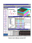


![2.8 conexión de varios servidores xt[2]](http://vs1.manualzilla.com/store/data/006305919_1-9948e093384d4040cdf0f68f445b7f43-150x150.png)